The $B^{0}\to J/\psi f_{0}(1370,1500,1710)$ decays: an opportunity for scalar glueball hunting

Abstract

The scalars $f_{0}$ closest to 1.5 GeV contain the mesons $f_{0}(1370)$, $f_{0}(1500)$ and $f_{0}(1710)$, and the latter two ones are usually viewed as the potential candidates for the scalar glueballs. In this work, by including the important contributions from the vertex corrections, we study the decays $B^{0}\to J/\psi f_{0}$ within the improved perturbative QCD approach and analyze the possible scalar glueball hunting. Together with the two mixing models, namely, $f_{0}(1500)(f_{0}(1710))$ being the primary scalar glueball in model I (II), and two classification scenarios, namely, $f_{0}$ being the $q\bar{q}$ excited (ground) states in scenario 1 (2), the branching fractions associated with their ratios for $B^{0}\to J/\psi f_{0}$ are evaluated comprehensively. The predictions with still large uncertainties in the considered two mixing models are roughly consistent with currently limited data, which indicates that both more rich data and more precise predictions are urgently demanded to figure out the scalar glueball clearly in the future. Moreover, several interesting ratios between the branching fractions of $B^{0}\to J/\psi f_{0}(\to\pi^{+}\pi^{-}/K^{+}K^{-})$ and $B^{0}\to J/\psi\rho^{0}/\phi(\to\pi^{+}\pi^{-}/K^{+}K^{-})$ that could help us to understand the nature of scalar $f_{0}$ are defined and predicted theoretically. These ratios should be examined in future experiments.

I Introduction

Quantum ChromoDynamics (QCD) Fritzsch:1972jv ; Gross:2022hyw , a theory simultaneously involving perturbative asymptotic freedom and nonperturbative color confinement, predicts firmly the existence of gluonic bound states while without any constituent quarks Fritzsch:1975tx , namely, the glueballs. However, the definite identification of the glueballs has been proven challenging and still remains a longstanding problem in hadron physics. Nevertheless, tremendous efforts from both the theoretical and experimental sides have been devoted to this subject. Some comprehensive reviews on the current status of glueballs could be seen in, e.g., Refs. Klempt:2007cp ; Ochs:2013gi ; Chen:2022asf , and more references therein.

So far, based on Lattice QCD (LQCD) simulations, it is commonly believed that the lightest glueball state should be a scalar with quantum number $J^{PC}=0^{++}$ and with mass around 1.5-1.8 GeV Bali:1993fb ; Chen:1994uw ; Morningstar:1999rf ; Vaccarino:1999ku ; Lee:1999kv ; Liu:2000ce ; Liu:2001je ; Ishii:2001zq ; Chen:2005mg ; Loan:2005ff ; Richards:2010ck ; Gregory:2012hu ; Gui:2012gx . While, three scalar resonances closet to this mass region, i.e., $f_{0}(1370)$, $f_{0}(1500)$ and $f_{0}(1710)$, could be found in the particle list provided by the Particle Data Group (PDG) ParticleDataGroup:2020ssz ( Henceforth, we will adopt $f_{0}$ to generally denote these three scalars, unless otherwise stated.). But, only one of them would be the potential candidate, that is, primarily a scalar glueball . It is due to the fact that the lowest-lying scalar glueball has the same quantum number as QCD vacuum, and thereby mixes with scalar quarkonium Lu:2013jj . Hence, the $q\bar{q}$ assignment cannot accommodate all these three $f_{0}$ states Cheng:2006hu ; Cheng:2015iaa .

Accompanied with the discovery of $f_{0}(1370)$ and $f_{0}(1500)$ CrystalBarrel:1994doj ; Amsler:1995gf ; CrystalBarrel:1996wfh , Amsler and Close proposed initially a flavor mixing scheme with the scalar quarkonia $N(\equiv(u\bar{u}+d\bar{d})/\sqrt{2})$ and $S(\equiv s\bar{s}$) and the scalar glueball $G$ to produce the observed $f_{0}(1370)$, $f_{0}(1500)$ and $f_{0}(1710)$ Amsler:1995tu ; Amsler:1995td . And, two of them can be considered as $q\bar{q}$ mesons with glue content, and the rest one would be primarily the scalar glueball but with (a) few scalar quarkonia. The $f_{0}$ state can then be expressed as follows,

$$|f_{0}\rangle = \alpha_{1}|N\rangle+\alpha_{2}|S\rangle+\alpha_{3}|G\rangle\;,$$ (1)

with coefficients $\alpha_{i}(i=1,2,3)$ measuring different kinds of contents in $f_{0}$, and satisfying approximately the following normalization Lu:2013jj ,

$${|\alpha_{1}|}^{2}+{|\alpha_{2}|}^{2}+{|\alpha_{3}|}^{2}\simeq 1.$$ (2)

In the past decades, numerous follow-up studies have been made with different mixing schemes, for example, in Refs. Lee:1999kv ; Li:2000yn ; Close:2000yk ; Li:2000cj ; Close:2001ga ; Giacosa:2004ug ; Close:2005vf ; Giacosa:2005zt ; Giacosa:2005qr ; Cheng:2006hu ; Chatzis:2011qz ; Gui:2012gx ; Janowski:2013uga ; Janowski:2014ppa ; Cheng:2015iaa ; Frere:2015xxa ; Vento:2015yja ; Noshad:2018afw ; Guo:2020akt . But, most of these studies focused on the productions of $f_{0}$ in $J/\psi$ and decay properties of $f_{0}$ in the low energy region.

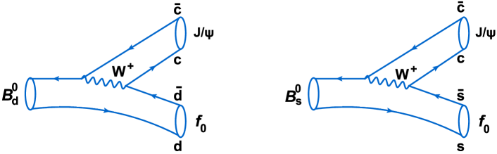
In contrast to the decays of $J/\psi$ or charmed mesons, the productions of $f_{0}$ in $B$-meson (including doubly heavy $B_{c}$ meson) decays can be remarkable and provide additional information of high statistics, because of the larger phase space and an apparent suppression of higher spin ($J=2$) states Minkowski:2004xf ; He:2006qk ; Chen:2007uq ; Wang:2009rc ; Wang:2009cb ; Ochs:2013gi ; Lu:2013jj ; He:2015owa . Particularly, the experiments at $B$ factories, Large Hadron Collider, and Belle-II have produced a large amount of events of $B$ decays, in which the scalar particles have been detected ever since the first observation of $f_{0}(980)$ by Belle and BABAR Collaborations Abe:2002av ; Aubert:2003mi . Therefore, the study of $f_{0}$’s production in $B$ decays could provide an effective way to clarify the intrinsic structure of scalars and help to figure out the gluon component inside, for example, the neutral $B$-meson decays into $f_{0}$ plus charmonia, in particular, in light of the recent data on $B^{0}\to J/\psi f_{0}(\to\pi^{+}\pi^{-}/K^{+}K^{-})$ decays ParticleDataGroup:2020ssz ; HFLAV:2022pwe . Here, $B^{0}$ includes $B_{d}^{0}$ and $B_{s}^{0}$. The differentiation on flavor composition would be possible from the decays $B_{d}^{0}\to J/\psi f_{0}$ and $B_{s}^{0}\to J/\psi f_{0}$ allowing for an isolation of the scalar $N(d\bar{d})$ and $S(s\bar{s})$ components of $f_{0}$ correspondingly Ochs:2013gi , as illustrated in Fig. 1. Therefore, the coefficients for related scalar quarkonia could be determined in $f_{0}$ through the $B^{0}\to J/\psi f_{0}$ branching fractions (${\cal B}$), which may be useful for conjecturing the fractions of scalar glueball .

Figure 1: (Color online) Leading quark-level Feynman diagrams for $B^{0}\to J/\psi f_{0}$

Experimentally, the decays $B_{s}^{0}\to J/\psi f_{0}(1370)$ and $B_{s}^{0}\to J/\psi f_{0}(1500)$ have been measured by Belle and Large Hadron Collider-beauty (LHCb) Collaborations through $f_{0}\to\pi^{+}\pi^{-}$ Belle:2011phz ; LHCb:2012ae ; LHCb:2014ooi . Their branching fractions are reported as follows ParticleDataGroup:2020ssz ,

$${\cal B}(B_{s}^{0}\to J/\psi f_{0}(1370),f_{0}\to\pi^{+}\pi^{-}) = (0.34^{+0.14}_{-0.15})\times 10^{-4}\;,\;\;\ ({\rm Belle})$$ (3)

$${\cal B}(B_{s}^{0}\to J/\psi f_{0}(1370),f_{0}\to\pi^{+}\pi^{-}) = (4.4_{-4.0}^{+0.6})\times 10^{-5}\;,\;\;\;\;\;\;({\rm LHCb})$$ (4)

$${\cal B}(B_{s}^{0}\to J/\psi f_{0}(1500),f_{0}\to\pi^{+}\pi^{-}) = (2.04_{-0.24}^{+0.32})\times 10^{-5}\;.\;\;\;\;({\rm LHCb})$$ (5)

Of course, the large uncertainties are expected to be reduced by the upgraded LHCb and the on-going Belle-II experiments.

Theoretically, the decays $B^{0}\to J/\psi f_{0}$ have been investigated partially in Refs. Xie:2014gla ; Wang:2009rc ; Wang:2009cb ; Lu:2013jj , in particular,

• Under the approach based on chiral unity theory, the decays $B^{0}\to J/\psi f_{0}(1370)$ and $B^{0}\to J/\psi f_{0}(1710)$ were studied with the assumptions of the scalar glueball $f_{0}(1500)$. The ratios among their decay widths were also predicted with large uncertainties as follows Xie:2014gla ,

  $$\frac{\Gamma(B_{d}^{0}\to J/\psi f_{0}(1370))}{\Gamma(B_{d}^{0}\to J/\psi f_{0}(1710))} = 6.2\pm 1.6\;,$$

  $$\frac{\Gamma(B_{d}^{0}\to J/\psi f_{0}(1710))}{\Gamma(B_{s}^{0}\to J/\psi f_{0}(1710))} = (7.7\pm 1.9)\times 10^{-3}\;,$$ (6)

  $$\frac{\Gamma(B_{s}^{0}\to J/\psi f_{0}(1370))}{\Gamma(B_{s}^{0}\to J/\psi f_{0}(1710))} = (1.1\pm 0.3)\times 10^{-2}\;.$$

• In Refs. Wang:2009rc ; Wang:2009cb , using naive factorization and the Wilson coefficient $a_{2}$ extracted from $B_{d}^{0}\to J/\psi K_{S}^{0}$, the authors estimated the branching fractions of $B_{d}^{0}\to J/\psi f_{0}(N)$ and $B_{s}^{0}\to J/\psi f_{0}(S)$ by classifying $f_{0}$ states in two scenarios as,

  $${\cal B}(B_{d}^{0}\to J/\psi f_{0}(N)) \simeq \left\{\begin{array}[]{ll}(23^{+12}_{-14})\times 10^{-6}&\vspace{0.12cm}\\ (10^{+7}_{-5})\times 10^{-5}&\\ \end{array}\right.\;,$$ (9)

  $${\cal B}(B_{s}^{0}\to J/\psi f_{0}(S)) \simeq \left\{\begin{array}[]{ll}(6.5^{+4.0}_{-4.5})\times 10^{-4}&\vspace{0.12cm}\\ (3.5^{+2.3}_{-1.4})\times 10^{-3}&\\ \end{array}\right.\;.$$ (12)

  The authors also claimed that such large branching fractions would offer an opportunity to probe the structures of scalars and to solve the mixing problem between the scalar mesons with the available data in the future, which can serve for inferring about the glueball component in principle.

• The authors further focused on the potential identification of a scalar glueball by extracting the coefficient $\alpha_{1}$ in $B_{d}^{0}\to J/\psi f_{0}$ or $\alpha_{2}$ in $B_{s}^{0}\to J/\psi f_{0}$ based on SU(3) flavor symmetry and naive factorization, but the definite conclusion could not be drew Lu:2013jj .

In this work, we will study the decays $B^{0}\to J/\psi f_{0}$ in a comprehensive manner by employing the perturbative QCD(PQCD) approach Keum:2000ph ; Keum:2000wi ; Lu:2000em ; Lu:2000hj at the known next-to-leading order (NLO) accuracy to analyze the opportunity for identifying the possible scalar glueball potentially. Different from QCD factorization approach Beneke:1999br ; Du:2000ff and soft-collinear effective theory Bauer:2000yr based on the collinear factorization theorem, the PQCD approach within the framework of $k_{T}$ factorization theorem has advantages to deal with the nonfactorizable emission ($nfe$) diagrams and the annihilation ones , besides the factorizable emission ($fe$) contributions. By keeping the non-vanishing transverse momentum $k_{T}$ of quarks, the PQCD approach avoid the end-point divergences. Furthermore, with resummation techniques, two resultant factors are produced to guarantee the removal of the end-point singularities, which makes PQCD calculations of hadronic matrix elements effective and reliable. One called Sudakov factor, $e^{-S(t)}$ with $t$ the running scale at the largest energy, could strongly suppress the soft dynamics via resumming the double logarithms in the small $k_{T}$ (or large ${\bf b}$, the conjugate space coordinate of transverse momentum $k_{T}$) region with $k_{T}$ resummation Botts:1989nd ; Li:1992nu . And another one is called jet function, $S_{t}(x)$ with $x$ the momentum fraction of valence quark in a meson, which could largely smear the end-point divergences through resumming the double logarithms in the small $x$ region with threshold resummation Li:2001ay ; Li:2002mi . The detailed expressions of $S_{t}(x)$ and $e^{-S(t)}$ are referred to the Refs. Li:2001ay ; Li:2002mi ; Botts:1989nd ; Li:1992nu ; Li:2003yj ; Liu:2018kuo . In recent years, several developments on the PQCD approach have been obtained, for a review, see, e.g. Cheng:2020fcx . Particularly, the newly derived Sudakov factor for $J/\psi$ by including the charm quark mass effects further improves the PQCD framework for $B$-meson decaying into charmonia plus light hadron(s) Liu:2018kuo ; Liu:2023kxr .

As presented in, e.g., Refs. Cheng:2000kt ; Song:2002gw ; Chen:2005ht ; Li:2006vq ; Beneke:2008pi ; Liu:2009yno ; Colangelo:2010wg ; Liu:2012ib ; Liu:2013nea ; Wang:2015uea ; Liu:2019ymi ; Yao:2022zom , the $B$-meson decays into a charmonium plus light hadrons are color-suppressed and should include the NLO contributions from vertex corrections and NLO Wilson coefficients to make predictions compatible with data. Therefore, associated with the newly derived Sudakov factor for charmonia Liu:2018kuo ; Liu:2023kxr , we will comprehensively evaluate the branching fractions and their interesting ratios in $B^{0}\to J/\psi f_{0}$ at the NLO accuracy, together with two available models for $f_{0}$’s mixing, i.e., $f_{0}(1500)(f_{0}(1710))$ is viewed as the primary scalar glueball in model I (II), and two possible scenarios for $f_{0}$’s classification, i.e., $f_{0}$ is regarded as the two-quark first excited (lowest-lying) mesons in scenario 1 (2). The predicted branching fractions could provide a natural filter of quarkonia $N$ or $S$ and the scalar glueball could be deduced from the ratios among those branching fractions. On the other hand, analogous to the channel $B_{s}^{0}\to J/\psi f_{0}(980)$, the decays $B_{s}^{0}\to J/\psi f_{0}$ with no needs of angular analysis could also contribute clearly to the CP-violating parameter, namely, the $B_{s}^{0}$-$\bar{B}_{s}^{0}$ mixing phase $\beta_{s}$, which is sensitive to the possible new physics beyond the standard model.

This paper is organized as follows. In Sect. II, we give a brief review on the $f_{0}$’s mixing and classifications that will be adopted. Perturbative calculations of the $B^{0}\to J/\psi f_{0}$ decay amplitudes in the PQCD approach are also collected in this section. In Sect. III, we perform the numerical evaluations and remark on the theoretical results phenomenologically. A summary of this work is finally given in Sect. IV.

II PERTURBATIVE QCD CALCULATIONs

II.1 Classification and flavor mixing of $f_{0}$

A well-known fact is that the inner structure of light scalars is not yet well established theoretically (for a review, see, e.g., Refs. Klempt:2007cp ; Ochs:2013gi ; Chen:2022asf ). Many explanations to their possible contents have been proposed, for example, $\bar{q}q$, $\bar{q}\bar{q}qq$, meson-meson bound states or even supplemented with a scalar glueball. It seems that they are not made of one simple component but are the superpositions of the above mentioned ones. Actually, different scenarios tend to provide different predictions on the production and decay of light scalars, which are helpful to determine the dominant component.

Nowadays, in the spectroscopy study, many light scalar states have been discovered experimentally but their underlying structures are still remaining basically unknown. According to the particles collected by PDG ParticleDataGroup:2020ssz , the light scalars below or near 1 GeV, including $a_{0}(980)$, $K^{*}_{0}(700)({\rm or}~{}\kappa)$, $f_{0}(500)({\rm or}~{}\sigma)$, and $f_{0}(980)$, are usually viewed to form an SU(3) flavor nonet; while the light scalars around 1.5 GeV, including $a_{0}(1450)$, $K^{*}_{0}(1430)$, $f_{0}(1370)$, and $f_{0}(1500)/f_{0}(1710)$, form another nonet.

Presently, it is generally accepted that the light scalars can be considered as $q\bar{q}$-mesons in two scenarios Cheng:2005nb , namely,

• Scenario 1 (S1): the light scalars in the aforementioned former nonet are treated as the lowest-lying $q\bar{q}$ states, and those in the latter nonet are the corresponding first excited states.

• Scenario 2 (S2): the light scalars in the aforementioned latter nonet are viewed as the ground $q\bar{q}$ states and the corresponding first excited ones are believed to lie between $(2.0\sim 2.3)$ GeV. While those in the former nonet have to be four-quark bound states.

Therefore, in the two-quark picture, the scalars $f_{0}(1370)$ and $f_{0}(1500)/f_{0}(1710)$ considered in this work will be $q\bar{q}$ nonet corresponding to the first excited states in S1 while the lowest-lying states in S2.

Now, let us briefly review the status about the scalar quarkonia and glueball mixing schemes, namely, $N$-$S$-$G$ mixing, for the scalars $f_{0}(1370)$, $f_{0}(1500)$, and $f_{0}(1710)$. As aforementioned, ever since the pioneering works on the mixing of the scalar quarkonia and the scalar glueball by Amsler and Close, a number of schemes have been proposed generally by combining the experimental measurements and LQCD calculations. A consensus has been reached that $f_{0}(1370)$ does not have a sizable $G$ component and is predominated by the scalar quarkonium $N$, which is consistent with the fact that the $f_{0}(1370)$ does not couple strongly to $K\bar{K}$  Fritzsch:1972jv , though it is quite controversial that which of the two remaining isoscalars, i.e., $f_{0}(1500)$ and $f_{0}(1710)$, is primarily the scalar glueball.

Among all the available mixing schemes in the literature, two different models are proposed to describe the $N$-$S$-$G$ mixing. That is, $f_{0}(1500)$ is primarily a scalar glueball while $f_{0}(1710)$ is governed by the scalar quarkonium $S$ in model I ($M_{\rm I}$), and, $f_{0}(1710)$ is prominently a scalar glueball while $f_{0}(1500)$ is dominated by the scalar quarkonium $S$ in model II ($M_{\rm{II}}$). By fitting the masses, namely, the scalar $N$-quarkonium mass $m_{N}$, the scalar $S$-quarkonium mass $m_{S}$ and the scalar glueball mass $m_{G}$, and analyzing their branching fractions in strong decays, the matrix elements of $f_{0}(1370)$-$f_{0}(1500)$-$f_{0}(1710)$ mixing are constrained. But, the magnitude and sign of the mixing matrix elements are usually different even if in the same kind of model. It seems that the current status of the mixing schemes is highly complicated and evidently far from satisfactory, implying that the definite determination of the matrices for $N$-$S$-$G$ mixing is still a tough task.

Despite all that, due to no interferences between $B_{d}^{0}\to J/\psi f_{0}(N)$ and $B_{s}^{0}\to J/\psi f_{0}(S)$, the sign in the mixing matrices does not affect the analyses in this work and will be left for future studies involving significant interferences. Then we just take the magnitude of the mixing matrices into account. To date, the mixing matrices have been studied mostly by following various measurements and LQCD calculations with good precision. Therefore, in light of the increasing accuracy of experimental measurements and LQCD evaluations, it is better for us to consider the mixing schemes in the literature since 2000.

For the sake of objectiveness in the following calculations and analyses, averaging the matrix elements Hsiao:2014dva collected from various works  in each kind of model is preferred. Explicitly, the averaged matrix elements $\bar{\alpha}_{i}(i=1,2,3)$ for the scalar quarkonia $N$ and $S$ and the scalar glueball $G$ can be defined as follows,

$$\bar{\alpha}_{i} = \Biggl{(}\sum_{n}{|\alpha_{i}|}_{n}\Biggr{)}/n\;,$$ (13)

where $n$ is the number of mixing matrices quoted in this study. Notice that, only the central values of matrix elements $\alpha_{i}$ will be quoted here for convenience. In order to estimate the theoretical errors induced by the mixing matrix elements, the uncertainties $\Delta\bar{\alpha}_{i}$ are given by varying the averaged central values $\bar{\alpha}_{i}$ with ten percent. Therefore,

• For model I, by combining five mixing matrices in Refs. Close:2000yk ; Close:2001ga ; Giacosa:2004ug ; Giacosa:2005qr ; Chatzis:2011qz , the averaged mixing matrix with $f_{0}(1500)$ being the scalar glueball is obtained as follows,

  $$\left(\begin{array}[]{cccc}|f_{0}(1370)\rangle\\ |f_{0}(1500)\rangle\\ |f_{0}(1710)\rangle\\ \end{array}\right)=\left(\begin{array}[]{cccc}0.810\pm 0.081&0.164\pm 0.016&0.540\pm 0.054\\ 0.545\pm 0.055&0.230\pm 0.023&0.787\pm 0.079\\ 0.169\pm 0.017&0.942\pm 0.094&0.229\pm 0.023\\ \end{array}\right)\ \left(\begin{array}[]{cccc}|N\rangle\\ |S\rangle\\ |G\rangle\\ \end{array}\right)$$ (23)

  with the mass ordering $m_{S}>m_{G}>m_{N}$ and $m_{G}\simeq 1500$ MeV.

• For model II, by including five mixing matrices in Refs. Li:2000yn ; Chatzis:2011qz ; Janowski:2013uga ; Janowski:2014ppa ; Guo:2020akt , the averaged mixing matrix with $f_{0}(1710)$ being the scalar glueball can be read as follows,

  $$\left(\begin{array}[]{cccc}|f_{0}(1370)\rangle\\ |f_{0}(1500)\rangle\\ |f_{0}(1710)\rangle\\ \end{array}\right)=\left(\begin{array}[]{cccc}0.862\pm 0.086&0.331\pm 0.033&0.311\pm 0.031\\ 0.404\pm 0.040&0.869\pm 0.087&0.173\pm 0.017\\ 0.247\pm 0.025&0.275\pm 0.028&0.912\pm 0.091\\ \end{array}\right)\ \left(\begin{array}[]{cccc}|N\rangle\\ |S\rangle\\ |G\rangle\\ \end{array}\right)$$ (33)

  with the mass ordering $m_{G}>m_{S}>m_{N}$ and $m_{G}\simeq 1700$ MeV.

With them, we could then calculate the $B^{0}\to J/\psi f_{0}$ branching fractions in both models I and II to analyze the possibility for potential scalar glueball hunting. The explicit expressions and the information of citations about the quoted mixing matrices have been collected in Appendix A.

II.2 PQCD calculations of $B^{0}\to J/\psi f_{0}$

In the past two decades, PQCD approach, one of the popular factorization approaches on the basis of QCD, has been widely employed to study varieties of $B$-meson decays. Furthermore, the (quasi-) two-body $B$-meson decays into $J/\psi$ plus a light meson (or resonance)  Chen:2005ht ; Li:2006vq ; Liu:2009yno ; Liu:2012ib ; Liu:2013nea ; Wang:2015uea ; Liu:2019ymi ; Yao:2022zom have been studied in PQCD approach at the known NLO accuracy and most theoretical predictions are in agreement with the current data. Particularly, the PQCD study of the decays $B^{0}\to J/\psi f_{0}(500,980)$ Liu:2019ymi provided basically consistent predictions with the experimental measurements by different collaborations such as CDF, CMS, D0 and LHCb. Therefore, for investigating the decays $B^{0}\to J/\psi f_{0}(1370,1500,1710)$, it is natural to follow the same analytic calculations presented in Ref. Liu:2019ymi . As discussed in Liu:2019ymi , the factorization formulas $F_{fe}$ and $M_{nfe}$ from factorizable and nonfactorizable emission diagrams of $B^{0}\to J/\psi f_{0}$ are analogous to the longitudinal ones of $B^{0}\to J/\psi V$ Liu:2013nea . While, we need essential replacements of information from the vector meson to the $f_{0}$ appropriately. So, for simplicity, we will not present $F_{fe}$ and $M_{nfe}$ here for the decays $B^{0}\to J/\psi f_{0}$ explicitly. The interested readers can refer the related equations, e.g., Eqs. (37) and (40), in Liu:2013nea for detail.

For the decays $B^{0}\to J/\psi f_{0}$, the effective Hamiltonian $H_{\rm eff}$ could be written as Buchalla:1995vs

$$H_{\rm eff}\, = \,{G_{F}\over\sqrt{2}}\biggl{\{}V^{*}_{cb}V_{cq}\biggl{[}C_{1}(\mu)O_{1}^{c}(\mu)+C_{2}(\mu)O_{2}^{c}(\mu)\biggr{]}-V^{*}_{tb}V_{tq}\biggl{[}\sum_{i=3}^{10}C_{i}(\mu)O_{i}(\mu)\biggr{]}\biggr{\}}\;,$$ (34)

where the light quark $q=d$ or $s$, the Fermi constant $G_{F}=1.16639\times 10^{-5}{\rm GeV}^{-2}$. $V$ represents the Cabibbo-Kobayashi-Maskawa (CKM) matrix elements, and $C_{i}(\mu)$ are Wilson coefficients at the renormalization scale $\mu$. The local four-quark operators $O_{i}(i=1,\cdots,10)$ are listed in order:

1. (1) Tree operators

   $${\begin{array}[]{ll}\displaystyle O_{1}^{c}\,=\,(\bar{q}_{\alpha}c_{\beta})_{V-A}(\bar{c}_{\beta}b_{\alpha})_{V-A}\;,&\displaystyle O_{2}^{c}\,=\,(\bar{q}_{\alpha}c_{\alpha})_{V-A}(\bar{c}_{\beta}b_{\beta})_{V-A}\;,\end{array}}$$ (36)

2. (2) QCD penguin operators

   $${\begin{array}[]{ll}\displaystyle O_{3}\,=\,(\bar{q}_{\alpha}b_{\alpha})_{V-A}\sum_{q^{\prime}}(\bar{q}^{\prime}_{\beta}q^{\prime}_{\beta})_{V-A}\;,&\displaystyle O_{4}\,=\,(\bar{q}_{\alpha}b_{\beta})_{V-A}\sum_{q^{\prime}}(\bar{q}^{\prime}_{\beta}q^{\prime}_{\alpha})_{V-A}\;,\\ \displaystyle O_{5}\,=\,(\bar{q}_{\alpha}b_{\alpha})_{V-A}\sum_{q^{\prime}}(\bar{q}^{\prime}_{\beta}q^{\prime}_{\beta})_{V+A}\;,&\displaystyle O_{6}\,=\,(\bar{q}_{\alpha}b_{\beta})_{V-A}\sum_{q^{\prime}}(\bar{q}^{\prime}_{\beta}q^{\prime}_{\alpha})_{V+A}\;,\end{array}}$$ (39)

3. (3) Electroweak penguin operators

   $${\begin{array}[]{ll}\displaystyle O_{7}\,=\,\frac{3}{2}(\bar{q}_{\alpha}b_{\alpha})_{V-A}\sum_{q^{\prime}}e_{q^{\prime}}(\bar{q}^{\prime}_{\beta}q^{\prime}_{\beta})_{V+A}\;,&\displaystyle O_{8}\,=\,\frac{3}{2}(\bar{q}_{\alpha}b_{\beta})_{V-A}\sum_{q^{\prime}}e_{q^{\prime}}(\bar{q}^{\prime}_{\beta}q^{\prime}_{\alpha})_{V+A}\;,\\ \displaystyle O_{9}\,=\,\frac{3}{2}(\bar{q}_{\alpha}b_{\alpha})_{V-A}\sum_{q^{\prime}}e_{q^{\prime}}(\bar{q}^{\prime}_{\beta}q^{\prime}_{\beta})_{V-A}\;,&\displaystyle O_{10}\,=\,\frac{3}{2}(\bar{q}_{\alpha}b_{\beta})_{V-A}\sum_{q^{\prime}}e_{q^{\prime}}(\bar{q}^{\prime}_{\beta}q^{\prime}_{\alpha})_{V-A}\;,\end{array}}$$ (42)

in which, $\alpha$ and $\beta$ are the color indices and the notations $(\bar{q}^{\prime}q^{\prime})_{V\pm A}=\bar{q}^{\prime}\gamma_{\mu}(1\pm\gamma_{5})q^{\prime}$. The index $q^{\prime}$ in the summation of the above operators runs through $u,\;d,\;s$, $c$, and $b$. Here, we define the Wilson coefficients as

$$a_{1} = C_{2}+\frac{C_{1}}{3}\;,\qquad a_{2}=C_{1}+\frac{C_{2}}{3}\;,$$ (43)

$$a_{i} = C_{i}+\frac{C_{i+1}}{3}(i=3,5,7,9)\;,\qquad a_{j}=C_{j}+\frac{C_{j-1}}{3}(j=4,6,8,10)\;.$$ (44)

Figure 2: (Color online) Vertex corrections to $B^{0}\to J/\psi f_{0}$

Before proceeding, two remarks are presented necessarily as follows,

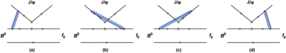
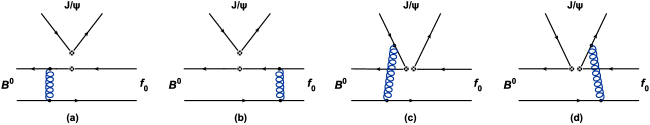
• In the literature, many works such as Refs. Cheng:2000kt ; Song:2002gw ; Chen:2005ht ; Li:2006vq ; Beneke:2008pi ; Liu:2009yno ; Colangelo:2010wg ; Liu:2012ib ; Liu:2013nea ; Wang:2015uea ; Liu:2019ymi ; Yao:2022zom have proved that the $B$-meson decays into charmonia plus light hadrons, the color-suppressed decay modes, usually receive the important NLO contributions, that is, vertex corrections. Hence, for the decays $B^{0}\to J/\psi f_{0}$, the related vertex corrections depicted in Fig. 2 will contribute. As pointed out in Cheng:2000kt , their effects will modify the Wilson coefficients in the factorizable emission diagrams Figs. 3(a) and 3(b) and further lead to a set of effective Wilson coefficients $\tilde{a}_{i}(i=2,3,5,7,9)$. The detailed expressions of $\tilde{a}_{i}$ are given in Liu:2019ymi , and no longer presented here.

• As stated in Liu:2013nea , when we consider the PQCD calculation at the NLO accuracy, it is natural for us to include the NLO Wilson coefficients $C_{i}(m_{W})$ and the NLO renormalization group evolution matrix $U(t,m,\alpha)$ for the Wilson coefficient (see Eq. (7.22) in Buchalla:1995vs ) with the running coupling $\alpha_{s}(t)$ at two-loop,

  $$\alpha_{s}(t) = \frac{4\pi}{\beta_{0}\ln(t^{2}/\Lambda_{\rm QCD}^{2})}\cdot\biggl{\{}1-\frac{\beta_{1}}{\beta_{0}^{2}}\cdot\frac{\ln[\ln(t^{2}/\Lambda_{\rm QCD}^{2})]}{\ln(t^{2}/\Lambda_{\rm QCD}^{2})}\biggr{\}},$$ (45)

  where $\beta_{0}=(33-2N_{f})/3$ and $\beta_{1}=(306-38N_{f})/3$, instead of the leading order (LO) elements such as LO Wilson coefficients $C_{i}(m_{W})$ and LO renormalization group evolution matrix $U(t,m)^{(0)}$, and LO running coupling $\alpha_{s}$. For the hadronic scale $\Lambda_{\rm QCD}$, the $\Lambda_{\rm QCD}^{(4)}=0.287$ GeV (0.326 GeV) could be obtained by using $\Lambda_{\rm QCD}^{(5)}=0.225$ GeV for the LO (NLO) case Buchalla:1995vs . For the hard scale $t$, the lower cut-off $\mu_{0}=1.0$ GeV is chosen Xiao:2008sw .

Figure 3: (Color online) Leading order Feynman diagrams for $B^{0}\to J/\psi f_{0}$ in the PQCD approach

By taking various contributions from Feynman diagrams shown in Figs. 2 and 3 into consideration, the decay amplitudes of $B_{d}^{0}\to J/\psi f_{0}(N)$ and $B_{s}^{0}\to J/\psi f_{0}(S)$ could thus be written as

$$\sqrt{2}A(B_{d}^{0}\to J/\psi f_{0}(N)) = F_{fe}^{N}f_{J/\psi}\biggl{\{}V_{cb}^{\ast}V_{cd}\tilde{a}_{2}-V_{tb}^{\ast}V_{td}\biggl{(}\tilde{a}_{3}+\tilde{a}_{5}+\tilde{a}_{7}+\tilde{a}_{9}\biggr{)}\biggr{\}}$$ (46)

$$+M_{nfe}^{N}\biggl{\{}V_{cb}^{\ast}V_{cd}C_{2}-V_{tb}^{\ast}V_{td}\biggl{(}C_{4}-C_{6}-C_{8}+C_{10}\biggr{)}\biggr{\}}\;,$$

and

$$A(B_{s}^{0}\to J/\psi f_{0}(S)) = F_{fe}^{S}f_{J/\psi}\biggl{\{}V_{cb}^{\ast}V_{cs}\tilde{a}_{2}-V_{tb}^{\ast}V_{ts}\biggl{(}\tilde{a}_{3}+\tilde{a}_{5}+\tilde{a}_{7}+\tilde{a}_{9}\biggr{)}\biggr{\}}$$ (47)

$$+M_{nfe}^{S}\biggl{\{}V_{cb}^{\ast}V_{cs}C_{2}-V_{tb}^{\ast}V_{ts}\biggl{(}C_{4}-C_{6}-C_{8}+C_{10}\biggr{)}\biggr{\}}\;,$$

where the four functions $(F_{fe}^{N},M_{nfe}^{N},F_{fe}^{S},M_{nfe}^{S})$ denote the factorization formulas arising from factorizable and nonfactorizable emission diagrams in the $B_{d}^{0}\to J/\psi f_{0}(N)$ and $B_{s}^{0}\to J/\psi f_{0}(S)$ modes respectively.

According to Eq. (1), the $B^{0}\to J/\psi f_{0}$ decay amplitudes could then be written explicitly with $A(B_{d}^{0}\to J/\psi f_{0}(N))$ and $A(B_{s}^{0}\to J/\psi f_{0}(S))$ as follows

$${\cal A}(B_{d}^{0}\to J/\psi f_{0}) = A(B_{d}^{0}\to J/\psi f_{0}(N))\cdot\alpha_{1}\;,$$ (48)

$${\cal A}(B_{s}^{0}\to J/\psi f_{0}) = A(B_{s}^{0}\to J/\psi f_{0}(S))\cdot\alpha_{2}\;,$$ (49)

where $\alpha_{1}$ and $\alpha_{2}$ will vary depending on the final states $f_{0}(1370)$, $f_{0}(1500)$, and $f_{0}(1710)$ correspondingly.

III Numerical results and discussions

In this section, we will perform the numerical calculations based on the given decay amplitudes to predict the branching fractions and their relative ratios for the decays $B^{0}\to J/\psi f_{0}$. Meanwhile, the phenomenological discussions on the potential scalar glueball hunting combining with the related numerical results will be presented. In numerical calculations, central values of the input parameters will be used implicitly unless otherwise stated.

First of all, several comments on the nonperturbative inputs are presented in order:

• (1) In light of the good consistency between experimental measurements and PQCD predictions for, e.g., $B\to J/\psi V$ Liu:2013nea , $B^{0}\to J/\psi f_{0}(500,980)$ Liu:2019ymi , and so forth, the wave functions in association with the distribution amplitudes, decay constants and mesonic masses of $B^{0}$ and $J/\psi$ in this work will be adopted same as those in Refs. Chen:2005ht ; Li:2006vq ; Liu:2009yno ; Liu:2012ib ; Liu:2013nea ; Liu:2019ymi ; Yao:2022zom , but with updated $B^{0}$-meson lifetimes, i.e., $\tau_{B_{d}^{0}}=1.519\ \rm ps$ and $\tau_{B_{s}^{0}}=1.516\ \rm ps$ ParticleDataGroup:2020ssz .

• (2) For the wave functions and distribution amplitudes of scalar $N$ and $S$, we also take the same forms as those in the studies of $B^{0}\to J/\psi f_{0}(500,980)$ Liu:2019ymi , but replacing the masses, decay constants and Gegenbauer moments of $f_{0}$ Cheng:2005nb ; Li:2008tk considered in this work correspondingly. Their values have been calculated in QCD sum rule at the renormalization scale $\mu=1$ GeV in two different scenarios:

  • (a) For the scalar decay constants (in units of GeV) of $N$ and $S$, because of no available experimental measurements and QCD sum rule/LQCD evaluations about their values currently, we adopt $\bar{f}_{a_{0}(1450)}$ and $\bar{f}_{f_{0}(1500)}$ as $\bar{f}_{N}$ and $\bar{f}_{S}$ approximately.

    $$\bar{f}_{N} = \biggl{\{}\begin{array}[]{cc}-0.280\pm 0.030\qquad({\rm S1})\\ \hskip 9.10486pt0.460\pm 0.050\qquad({\rm S2})\end{array}\;,$$ (52)

    $$\bar{f}_{S} = \biggl{\{}\begin{array}[]{cc}-0.255\pm 0.030\qquad({\rm S1})\\ \hskip 9.10486pt0.490\pm 0.050\qquad({\rm S2})\end{array}\;.$$ (55)

    Notice that, because of the charge conjugation invariance or the conservation of the vector current, the neutral scalars cannot be produced via vector current, which consequently results in the zero vector decay constants, i.e., $f_{N}=f_{S}=0$ Cheng:2005nb .

  • (b) For the Gegenbauer moments $B_{1}$ and $B_{3}$ in leading twist distribution amplitudes, we firstly assume $B_{1,3}^{f_{0}(1500)}$ as $B_{1,3}^{S}$, then obtain the values of $B_{1,3}^{N}$ according to the relation $B_{1,3}^{S}\simeq 0.8B_{1,3}^{N}$ Cheng:2005ye . So, we have

    $$B_{1}^{N} = \biggl{\{}\begin{array}[]{cc}\hskip 9.10486pt1.00\pm 0.50\qquad\ ({\rm S1})\\ -0.60\pm 0.14\qquad\ ({\rm S2})\end{array}\;,$$ (58)

    $$B_{1}^{S} = \biggl{\{}\begin{array}[]{cc}\hskip 9.10486pt0.80\pm 0.40\qquad\ ({\rm S1})\\ -0.48\pm 0.11\qquad\ ({\rm S2})\end{array}\;,$$ (61)

    $$B_{3}^{N} = \biggl{\{}\begin{array}[]{cc}-1.65\pm 0.18\qquad\ ({\rm S1})\\ -0.46\pm 0.25\qquad\ ({\rm S2})\end{array}\;,$$ (64)

    $$B_{3}^{S} = \biggl{\{}\begin{array}[]{cc}-1.32\pm 0.14\qquad\ ({\rm S1})\\ -0.37\pm 0.20\qquad\ ({\rm S2})\end{array}\;.$$ (67)

  Moreover, for masses of the scalar quarkonia and the physical states, we adopt the values (in units of GeV) as: $m_{f_{0}(1370)}=1.350$, $m_{f_{0}(1500)}=1.506$, $m_{f_{0}(1710)}=1.704$ ParticleDataGroup:2020ssz , $m_{N}=1.304$ and $m_{S}=1.682$ in $M_{\rm I}$ Close:2005vf , and $m_{N}=1.474$ and $m_{S}=1.496$ in $M_{\rm II}$ Cheng:2015iaa , respectively. The necessary remark for $m_{f_{0}(1370)}$ is that we approximately take the central value $1350$ MeV based on the data, namely, 1200-1500 MeV provided by PDG, though the very existence of $f_{0}(1370)$ has long been questionable (see Refs. Bugg:2007ja ; Klempt:2007cp ; Ochs:2013gi for more detailed discussions) .

• (3) For the CKM matrix elements, we adopt the Wolfenstein parameterization up to $\mathcal{O}(\lambda^{5})$ Wolfenstein:1983yz with the four updated parameters ParticleDataGroup:2020ssz ,

  $$A=0.790,\quad\lambda=0.22650,\quad\bar{\rho}=0.141_{-0.017}^{+0.016},\quad\bar{\eta}=0.357_{-0.011}^{+0.011}.$$ (68)

  in which $\bar{\rho}\equiv\rho(1-\frac{\lambda^{2}}{2})$ and $\bar{\eta}\equiv\eta(1-\frac{\lambda^{2}}{2})$.

With the decay amplitudes ${\cal A}(B^{0}\to J/\psi f_{0})$ given in Eqs. (48) and (49), the branching fraction for the decay $B^{0}\to J/\psi f_{0}$ is given as follows,

$${\cal B}(B^{0}\to J/\psi f_{0}) \equiv \tau_{B^{0}}\cdot\Gamma(B^{0}\to J/\psi f_{0})$$ (69)

$$= \tau_{B^{0}}\cdot\frac{G_{F}^{2}m^{3}_{B^{0}}}{32\pi}\cdot\Phi(r_{J/\psi},r_{f_{0}})\cdot|{\cal A}(B^{0}\to J/\psi f_{0})|^{2}\;,$$

where $\tau_{B^{0}}$ is the lifetime of $B^{0}$-meson and $\Phi(r_{J/\psi},r_{f_{0}})$ stands for the phase space factor of $B^{0}\to J/\psi f_{0}$ with $r_{J/\psi}=m_{J/\psi}/m_{B^{0}}$ and $r_{f_{0}}=m_{f_{0}}/m_{B^{0}}$, $\Phi(x,y)\equiv\sqrt{[1-(x+y)^{2}]\cdot[1-(x-y)^{2}]}$ Fleischer:2011au .

Now we calculate the $B^{0}\to J/\psi f_{0}$ branching fractions in PQCD approach at NLO level. The numerical results within two different scenarios in both models I and II are presented in Table 1. Furthermore, we sequentially list the dominant errors arising from theoretical uncertainties of the shape parameter $\omega_{B_{d}^{0}}=0.40\pm 0.04$ GeV or $\omega_{B_{s}^{0}}=0.50\pm 0.05$ GeV in the $B^{0}$-meson distribution amplitude, of the $J/\psi$-meson decay constant $f_{J/\psi}=0.405\pm 0.014$ GeV, of the Gegenbauer moments $B_{i}^{N,S}(i=1,3)$ and the scalar decay constants $\bar{f}_{N,S}$ (see Eqs. (55)-(67)) in the light-cone distribution amplitudes of scalar quarkonia $N$ and $S$, and of the possibly higher order contributions by simply varying the running hard scale $t_{max}$, i.e., from $0.8t$ to $1.2t$, in the hard kernel.

Table 1: The branching fractions for $B^{0}\to J/\psi f_{0}$ with PQCD approach in both models I and II. The upper (lower) entry corresponds to $f_{0}$ in scenario 1 (2) at every line.

Decay modes	model I	model II
$B_{d}^{0}\to J/\psi f_{0}(1370)$	$\begin{array}[]{cc}(8.54^{+3.44+0.50+6.67+0.65+1.79}_{-2.48-0.49-1.89-1.27-1.62})\times 10^{-6}\\ (3.65^{+1.17+0.47+1.62+0.17+0.77}_{-0.84-0.42-1.41-0.27-0.69})\times 10^{-5}\end{array}$	$\begin{array}[]{cc}(1.04^{+0.43+0.06+0.74+0.08+0.22}_{-0.31-0.06-0.23-0.15-0.20})\times 10^{-5}\\ (4.38^{+1.44+0.57+1.90+0.22+0.92}_{-1.03-0.52-1.66-0.36-0.83})\times 10^{-5}\end{array}$
$B_{d}^{0}\to J/\psi f_{0}(1500)$	$\begin{array}[]{cc}(3.55^{+1.43+0.21+2.78+0.27+0.75}_{-1.03-0.20-0.79-0.53-0.67})\times 10^{-6}\\ (1.52^{+0.48+0.19+0.67+0.07+0.32}_{-0.35-0.18-0.59-0.12-0.29})\times 10^{-5}\end{array}$	$\begin{array}[]{cc}(2.10^{+0.87+0.12+1.49+0.15+0.43}_{-0.62-0.13-0.47-0.31-0.40})\times 10^{-6}\\ (8.84^{+2.89+1.15+3.82+0.44+1.83}_{-2.09-1.05-3.36-0.73-1.67})\times 10^{-6}\end{array}$
$B_{d}^{0}\to J/\psi f_{0}(1710)$	$\begin{array}[]{cc}(2.93^{+1.18+0.18+2.29+0.23+0.62}_{-0.85-0.16-0.64-0.43-0.56})\times 10^{-7}\\ (1.26^{+0.39+0.16+0.55+0.05+0.26}_{-0.30-0.15-0.49-0.10-0.24})\times 10^{-6}\end{array}$	$\begin{array}[]{cc}(6.73^{+2.80+0.41+4.80+0.51+1.43}_{-1.98-0.39-1.49-1.00-1.29})\times 10^{-7}\\ (2.84^{+0.93+0.37+1.23+0.14+0.60}_{-0.67-0.34-1.08-0.23-0.55})\times 10^{-6}\end{array}$
$B_{s}^{0}\to J/\psi f_{0}(1370)$	$\begin{array}[]{cc}(5.07^{+2.97+0.29+3.62+0.40+1.03}_{-1.90-0.27-1.23-0.77-0.94})\times 10^{-6}\\ (3.38^{+1.35+0.47+1.41+0.31+0.69}_{-0.92-0.42-1.25-0.36-0.63})\times 10^{-5}\end{array}$	$\begin{array}[]{cc}(1.90^{+1.09+0.11+1.53+0.16+0.40}_{-0.69-0.09-0.45-0.29-0.36})\times 10^{-5}\\ (1.30^{+0.51+0.18+0.30+0.11+0.27}_{-0.35-0.10-0.49-0.13-0.25})\times 10^{-4}\end{array}$
$B_{s}^{0}\to J/\psi f_{0}(1500)$	$\begin{array}[]{cc}(9.25^{+5.42+0.53+6.63+0.73+1.94}_{-3.46-0.50-2.25-1.39-1.76})\times 10^{-6}\\ (6.17^{+2.47+0.85+2.57+0.56+1.29}_{-1.67-0.77-2.28-0.66-1.17})\times 10^{-5}\end{array}$	$\begin{array}[]{cc}(1.22^{+0.69+0.06+0.97+0.10+0.25}_{-0.45-0.06-0.29-0.19-0.23})\times 10^{-4}\\ (8.32^{+3.23+1.12+3.55+0.69+1.74}_{-2.22-0.65-3.13-0.83-1.59})\times 10^{-4}\end{array}$
$B_{s}^{0}\to J/\psi f_{0}(1710)$	$\begin{array}[]{cc}(1.36^{+0.80+0.08+0.99+0.11+0.29}_{-0.51-0.07-0.33-0.20-0.25})\times 10^{-4}\\ (9.10^{+3.64+1.25+3.80+0.83+1.90}_{-2.46-1.14-3.36-0.98-1.73})\times 10^{-4}\end{array}$	$\begin{array}[]{cc}(1.07^{+0.62+0.06+0.86+0.09+0.23}_{-0.39-0.05-0.25-0.16-0.20})\times 10^{-5}\\ (7.32^{+2.86+0.99+3.14+0.62+1.57}_{-1.95-0.57-2.74-0.73-1.41})\times 10^{-5}\end{array}$

The last errors in the second and third columns of Table 1 stem from $10\%$ variations of the related coefficients for scalar quarkonia $N$ and $S$ in the mixing matrices. Due to their very smallness, the errors induced by the CKM matrix elements are negligible and not shown in the Table. It is obvious that the largest uncertainty arises from the least constrained hadronic parameters, i.e., the Gegenbauer moments $B_{i}^{N,S}(i=1,3)$ and the scalar decay constants $\bar{f}_{N,S}$, which are nonperturbative. Nevertheless, such large branching fractions of the decays $B^{0}\to J/\psi f_{0}$ within still large uncertainties generally around $10^{-6}\sim 10^{-3}$ would provide good probes to these parameters through the exhibited dynamics, because of the highly small penguin contributions. These numerical results are expected to be tested at LHCb and Belle-II experiments in the near future, which might provide useful constraints on the nonperturbative inputs and further lead to more reliable predictions. In principle, the future experimental confirmations on these large predictions could be helpful to determine the coefficients of the scalar quarkonia, namely, $\alpha_{1}$ for $N$ and $\alpha_{2}$ for $S$ in three considered scalars $f_{0}$.

• The decays $B^{0}\to J/\psi f_{0}(1370)$

  As seen from the PQCD branching fractions in Table 1, the consensus about dominated quarkonium $N$ of $f_{0}(1370)$ in both models I and II leads to the consistent ${\cal B}(B_{d}^{0}\to J/\psi f_{0}(1370))$ within uncertainties in each scenario, namely,

  $${\cal B}(B_{d}^{0}\to J/\psi f_{0}(1370))_{\rm S1} = \biggl{\{}\begin{array}[]{ll}(0.85^{+0.78}_{-0.38})\times 10^{-5}\qquad\ (M_{\rm I})\\ (1.04^{+0.89}_{-0.47})\times 10^{-5}\qquad\ (M_{\rm II})\end{array}\;,$$ (72)

  $${\cal B}(B_{d}^{0}\to J/\psi f_{0}(1370))_{\rm S2} = \biggl{\{}\begin{array}[]{ll}(3.65^{+2.20}_{-1.85})\times 10^{-5}\qquad\ (M_{\rm I})\\ (4.38^{+2.63}_{-4.92})\times 10^{-5}\qquad\ (M_{\rm II})\end{array}\;,$$ (75)

  which could be inferred from the close values $|\alpha_{1}^{M_{\rm I}}|=0.810\pm 0.081$ and $|\alpha_{1}^{M_{\rm II}}|=0.862\pm 0.086$ presented in Eqs. (23) and (33). These large results for the branching fractions of the decay $B_{d}^{0}\to J/\psi f_{0}(1370)$ are around $10^{-6}\sim 10^{-5}$ and could be accessible at the LHCb and Belle-II experiments. Meanwhile, it is worth mentioning that, though the $f_{0}(1370)$ is predominated by the scalar quarkonium $N$, the branching fractions of the decay $B_{s}^{0}\to J/\psi f_{0}(1370)$ are still large,

  $${\cal B}(B_{s}^{0}\to J/\psi f_{0}(1370))_{\rm S1} = \biggl{\{}\begin{array}[]{ll}(0.51^{+0.48}_{-0.26})\times 10^{-5}\qquad\ (M_{\rm I})\\ (1.90^{+1.93}_{-0.95})\times 10^{-5}\qquad\ (M_{\rm II})\end{array}\;,$$ (78)

  $${\cal B}(B_{s}^{0}\to J/\psi f_{0}(1370))_{\rm S2} = \biggl{\{}\begin{array}[]{ll}(3.38^{+2.14}_{-1.76})\times 10^{-5}\qquad\ (M_{\rm I})\\ (1.30^{+0.68}_{-0.67})\times 10^{-4}\qquad\ (M_{\rm II})\end{array}\;,$$ (81)

  which are capable of measuring at the on-going LHCb and Belle-II experiments.

  It is emphasized that, as presented in Eq. (4), this channel has been reported through $f_{0}(1370)\to\pi^{+}\pi^{-}$ while with surprisingly large uncertainties in the LHCb measurements, besides the evidence given by the Belle collaboration. As stated in Cheng:2015iaa , the narrow-width approximation (NWA) works provided that the resonance is not too broad. But, experimentally, the nature of $f_{0}(1370)$ is unknown till now. Thus, it looks unfeasible to make an efficient comparison straightforwardly for the branching fractions between the PQCD predictions and the LHCb measurements under NWA. Therefore, for future tests at relevant experiments, by taking the decays $B_{d}^{0}\to J/\psi\rho^{0}$ and $B_{s}^{0}\to J/\psi\phi$ as normalization, we can define the ratios between the branching fractions of $B^{0}\to J/\psi f_{0}$ and $B^{0}\to J/\psi\rho^{0}/\phi$. The updated values for ${\cal B}(B^{0}_{d}\to J/\psi\rho^{0})$ and ${\cal B}(B^{0}_{s}\to J/\psi\phi)$ in PQCD are available as $(2.98^{+0.81}_{-0.69})\times 10^{-5}$ and $(1.07^{+0.33}_{-0.29})\times 10^{-3}$ Yao:2022zom correspondingly. The values for the two ratios, namely, $R_{d}^{\rm Theo}[f_{03}/\rho]$ and $R_{s}^{\rm Theo}[f_{03}/\phi]$, with theoretical errors are then collected as,

  $$R_{d}^{\rm Theo}[f_{03}/\rho]_{\rm S1} \equiv \frac{{\cal B}(B_{d}^{0}\to J/\psi f_{0}(1370))_{\rm S1}}{{\cal B}(B_{d}^{0}\to J/\psi\rho^{0})}=\biggl{\{}\begin{array}[]{ll}0.287^{+0.201}_{-0.072}\qquad\ (M_{\rm I})\\ 0.349^{+0.222}_{-0.089}\qquad\ (M_{\rm II})\end{array}\;,$$ (84)

  $$R_{d}^{\rm Theo}[f_{03}/\rho]_{\rm S2} \equiv \frac{{\cal B}(B_{d}^{0}\to J/\psi f_{0}(1370))_{\rm S2}}{{\cal B}(B_{d}^{0}\to J/\psi\rho^{0})}=\biggl{\{}\begin{array}[]{ll}1.225^{+0.461}_{-0.434}\qquad\ (M_{\rm I})\\ 1.470^{+0.542}_{-0.512}\qquad\ (M_{\rm II})\end{array}\;,$$ (87)

  and

  $$R_{s}^{\rm Theo}[f_{03}/\phi]_{\rm S1} \equiv \frac{{\cal B}(B_{s}^{0}\to J/\psi f_{0}(1370))_{\rm S1}}{{\cal B}(B_{s}^{0}\to J/\psi\phi)}=\biggl{\{}\begin{array}[]{ll}0.005^{+0.003}_{-0.001}\qquad\ (M_{\rm I})\\ 0.018^{+0.013}_{-0.005}\qquad\ (M_{\rm II})\end{array}\;,$$ (90)

  $$R_{s}^{\rm Theo}[f_{03}/\phi]_{\rm S2} \equiv \frac{{\cal B}(B_{s}^{0}\to J/\psi f_{0}(1370))_{\rm S2}}{{\cal B}(B_{s}^{0}\to J/\psi\phi)}=\biggl{\{}\begin{array}[]{ll}0.032^{+0.011}_{-0.010}\qquad\ (M_{\rm I})\\ 0.121^{+0.045}_{-0.041}\qquad\ (M_{\rm II})\end{array}\;.$$ (93)

  The large ratios such as $R_{d}^{\rm Theo}[f_{03}/\rho]_{\rm S2,M_{I}}\in[0.791,1.686]$ and $R_{d}^{\rm Theo}[f_{03}/\rho]_{\rm S2,M_{II}}\in[0.958,2.012]$, and $R_{s}^{\rm Theo}[f_{03}/\phi]_{\rm S2,M_{II}}\in[0.080,0.166]$ need more experimental tests for further understanding the nature of $f_{0}(1370)$.

• The decays $B^{0}\to J/\psi f_{0}(1500)$

  Based on the results presented in Table 1, the PQCD predictions for ${\cal B}(B^{0}\to J/\psi f_{0}(1500))$ are collected as follows,

  $${\cal B}(B_{d}^{0}\to J/\psi f_{0}(1500))_{\rm S1} = \biggl{\{}\begin{array}[]{ll}(3.55^{+3.23}_{-1.57})\times 10^{-6}\qquad\ (M_{\rm I})\\ (2.10^{+1.79}_{-0.94})\times 10^{-6}\qquad\ (M_{\rm II})\end{array}\;,$$ (96)

  $${\cal B}(B_{d}^{0}\to J/\psi f_{0}(1500))_{\rm S2} = \biggl{\{}\begin{array}[]{ll}(1.52^{+0.91}_{-0.78})\times 10^{-5}\qquad\ (M_{\rm I})\\ (8.84^{+5.27}_{-4.48})\times 10^{-6}\qquad\ (M_{\rm II})\end{array}\;,$$ (99)

  and

  $${\cal B}(B_{s}^{0}\to J/\psi f_{0}(1500))_{\rm S1} = \biggl{\{}\begin{array}[]{ll}(0.93^{+0.88}_{-0.47})\times 10^{-5}\qquad\ (M_{\rm I})\\ (1.22^{+1.22}_{-0.62})\times 10^{-4}\qquad\ (M_{\rm II})\end{array}\;,$$ (102)

  $${\cal B}(B_{s}^{0}\to J/\psi f_{0}(1500))_{\rm S2} = \biggl{\{}\begin{array}[]{ll}(6.17^{+3.93}_{-3.22})\times 10^{-5}\qquad\ (M_{\rm I})\\ (8.32^{+5.27}_{-4.29})\times 10^{-4}\qquad\ (M_{\rm II})\end{array}\;,$$ (105)

  where the uncertainties from various sources have been added in quadrature. In principle, these large branching fractions around $10^{-6}\sim 10^{-4}$ are expected to be tested soon at the LHCb and Belle-II experiments. It is mentioned that, due to the comparable $N$-component of $f_{0}(1500)$ in models I and II, the $B_{d}^{0}\to J/\psi f_{0}(1500)$ decay rates are generally consistent with each other in each scenario. However, for the $B_{s}^{0}$ decay mode, the relation ${\cal B}(B_{s}^{0}\to J/\psi f_{0}(1500))_{M_{\rm II}}\sim 10\times{\cal B}(B_{s}^{0}\to J/\psi f_{0}(1500))_{M_{\rm I}}$ could be seen in both S1 and S2. It is indeed attributed to the fact that the $f_{0}(1500)$ state is assumed as the prominent glueball nature in model I while as the flavor octet structure in model II.

  The ratios $R_{d}^{\rm Theo}[f_{05}/\rho]$ and $R_{s}^{\rm Theo}[f_{05}/\phi]$ are then presented similarly as,

  $$R_{d}^{\rm Theo}[f_{05}/\rho]_{\rm S1} \equiv \frac{{\cal B}(B_{d}^{0}\to J/\psi f_{0}(1500))_{\rm S1}}{{\cal B}(B_{d}^{0}\to J/\psi\rho^{0})}=\biggl{\{}\begin{array}[]{ll}0.119^{+0.084}_{-0.030}\qquad\ (M_{\rm I})\\ 0.070^{+0.044}_{-0.018}\qquad\ (M_{\rm II})\end{array}\;,$$ (108)

  $$R_{d}^{\rm Theo}[f_{05}/\rho]_{\rm S2} \equiv \frac{{\cal B}(B_{d}^{0}\to J/\psi f_{0}(1500))_{\rm S2}}{{\cal B}(B_{d}^{0}\to J/\psi\rho^{0})}=\biggl{\{}\begin{array}[]{ll}0.510^{+0.190}_{-0.181}\qquad\ (M_{\rm I})\\ 0.297^{+0.109}_{-0.103}\qquad\ (M_{\rm II})\end{array}\;,$$ (111)

  and

  $$R_{s}^{\rm Theo}[f_{05}/\phi]_{\rm S1} \equiv \frac{{\cal B}(B_{s}^{0}\to J/\psi f_{0}(1500))_{\rm S1}}{{\cal B}(B_{s}^{0}\to J/\psi\phi)}=\biggl{\{}\begin{array}[]{ll}0.009^{+0.006}_{-0.003}\qquad\ (M_{\rm I})\\ 0.114^{+0.083}_{-0.033}\qquad\ (M_{\rm II})\end{array}\;,$$ (114)

  $$R_{s}^{\rm Theo}[f_{05}/\phi]_{\rm S2} \equiv \frac{{\cal B}(B_{s}^{0}\to J/\psi f_{0}(1500))_{\rm S2}}{{\cal B}(B_{s}^{0}\to J/\psi\phi)}=\biggl{\{}\begin{array}[]{ll}0.058^{+0.021}_{-0.019}\qquad\ (M_{\rm I})\\ 0.778^{+0.282}_{-0.255}\qquad\ (M_{\rm II})\end{array}\;,$$ (117)

  which could be helpful to study the inner structure of $f_{0}(1500)$ and to explore the fraction of glueball content.

  Actually, as mentioned in Sect. I, the LHCb Collaboration reported the experimental result of ${\cal B}(B_{s}^{0}\to J/\psi f_{0}(1500),f_{0}\to\pi^{+}\pi^{-})$ as $2.04^{+0.32}_{-0.24}\times 10^{-5}$. Then the ${\cal B}(B_{s}^{0}\to J/\psi f_{0}(1500))_{\rm Exp}$ could be easily derived with the data ${\cal B}(f_{0}(1500)\to\pi\pi)=(34.5\pm 2.2)\%$ ParticleDataGroup:2020ssz under NWA Cheng:2015iaa . With ${\cal B}(f_{0}(1500)\to\pi^{+}\pi^{-})=0.230\pm 0.015$ based on the isospin symmetry, we have

  $${\cal B}(B_{s}^{0}\to J/\psi f_{0}(1500))_{\rm Exp} = (8.87^{+0.76}_{-0.50})\times 10^{-5}\;.$$ (118)

  Experimentally, the $B_{s}^{0}\to J/\psi\phi$ branching fraction ParticleDataGroup:2020ssz is read as,

  $${\cal B}(B_{s}^{0}\to J/\psi\phi)_{\rm Exp} = (1.08^{+0.08}_{-0.08})\times 10^{-3}\;.$$ (119)

  Therefore, the ratio between the experimental branching fractions of $B_{s}^{0}\to J/\psi f_{0}(1500)$ and $B_{s}^{0}\to J/\psi\phi$ could be obtained as,

  $$R_{s}^{\rm Exp}[f_{05}/\phi] \equiv \frac{{\cal B}(B_{s}^{0}\to J/\psi f_{0}(1500))_{\rm Exp}}{{\cal B}(B_{s}^{0}\to J/\psi\phi)_{\rm Exp}}=0.082^{+0.002}_{-0.000}\;.$$ (120)

  By combining the branching fractions and the relative ratios, the results in the scheme of S1 with $M_{\rm II}$ seem closer to the values in Eqs. (118) and (120) derived from data than those in the scheme of S2 with $M_{\rm I}$. However, due to the still large uncertainties, the results in both of the above mentioned two schemes, i.e., S1 with $M_{\rm II}$ and S2 with $M_{\rm I}$, are consistent with the current data in 2$\sigma$ deviations. Certainly, it looks evidently that the values of ${\cal B}(B_{s}^{0}\to J/\psi f_{0}(1500))$ in both schemes of S1 with $M_{\rm I}$ and S2 with $M_{\rm II}$ are less favored by that in Eq. (118). The crosschecks from the Belle-II experiments for the decay $B_{s}^{0}\to J/\psi f_{0}(1500)(\to\pi^{+}\pi^{-})$ are thus urgently demanded.

  For comparing with the future measurements, we read the branching fractions for the decays $B^{0}\to J/\psi f_{0}(1500)(\to\pi^{+}\pi^{-})$ by using NWA Cheng:2015iaa . These theoretical predictions are collected in Table 2. Notice that the values for ${\cal B}(B_{s}^{0}\to J/\psi f_{0}(1500)(\to\pi^{+}\pi^{-}))$ in both schemes of S1 with $M_{\rm II}$ and S2 with $M_{\rm I}$ are well consistent with the current LHCb measurement within theoretical errors. The branching fractions in the order of $10^{-6}$ for the mode $B_{d}^{0}\to J/\psi f_{0}(1500)(\to\pi^{+}\pi^{-})$ are accessible in the on-going experiments at Belle-II and LHCb and await the near future examinations.

  Table 2: The branching fractions for the decays $B^{0}\to J/\psi f_{0}(1500)(\to\pi^{+}\pi^{-}/K^{+}K^{-})$ under NWA in the PQCD approach. The upper (lower) entry corresponds to $f_{0}(1500)$ in scenario 1 (2) at every line.

  Decay modes	model I	model II
  $B_{d}^{0}\to J/\psi f_{0}(1500)(\to\pi^{+}\pi^{-})$	$\begin{array}[]{cc}(8.17^{+7.45}_{-3.64})\times 10^{-7}\\ (3.50^{+2.11}_{-1.80})\times 10^{-6}\end{array}$	$\begin{array}[]{cc}(4.83^{+4.12}_{-2.18})\times 10^{-7}\\ (2.03^{+1.22}_{-1.04})\times 10^{-6}\end{array}$
  $B_{s}^{0}\to J/\psi f_{0}(1500)(\to\pi^{+}\pi^{-})$	$\begin{array}[]{cc}(2.13^{+2.04}_{-1.10})\times 10^{-6}\\ (1.42^{+0.91}_{-0.75})\times 10^{-5}\end{array}$	$\begin{array}[]{cc}(2.81^{+2.81}_{-1.43})\times 10^{-5}\\ (1.91^{+1.22}_{-0.99})\times 10^{-4}\end{array}$
  $B_{d}^{0}\to J/\psi f_{0}(1500)(\to K^{+}K^{-})$	$\begin{array}[]{cc}(1.51^{+1.39}_{-0.69})\times 10^{-7}\\ (6.46^{+3.94}_{-3.39})\times 10^{-7}\end{array}$	$\begin{array}[]{cc}(8.93^{+7.67}_{-4.13})\times 10^{-8}\\ (3.76^{+2.29}_{-1.96})\times 10^{-7}\end{array}$
  $B_{s}^{0}\to J/\psi f_{0}(1500)(\to K^{+}K^{-})$	$\begin{array}[]{cc}(3.93^{+3.78}_{-2.06})\times 10^{-7}\\ (2.62^{+1.70}_{-1.41})\times 10^{-6}\end{array}$	$\begin{array}[]{cc}(5.19^{+5.22}_{-2.69})\times 10^{-6}\\ (3.54^{+2.28}_{-1.87})\times 10^{-5}\end{array}$

  Analogously, as byproducts, the results for ${\cal B}(B^{0}\to J/\psi f_{0}(1500)(\to K^{+}K^{-}))$ could also be obtained with the data ${\cal B}(f_{0}(1500)\to K^{+}K^{-})=(4.25\pm 0.50)\%$ ParticleDataGroup:2020ssz on the basis of isospin symmetry. Using ${\cal B}(B_{s}^{0}\to J/\psi f_{0}(1500))_{\rm Exp}$ and ${\cal B}(f_{0}(1500)\to K^{+}K^{-})_{\rm Exp}$, the future measurement about ${\cal B}(B_{s}^{0}\to J/\psi f_{0}(1500)(\to K^{+}K^{-}))$ might be as approximately described under NWA,

  $${\cal B}(B_{s}^{0}\to J/\psi f_{0}(1500)(\to K^{+}K^{-}))_{\rm Exp} \simeq {\cal B}(B_{s}^{0}\to J/\psi f_{0}(1500))_{\rm Exp}\cdot{\cal B}(f_{0}(1500)\to K^{+}K^{-})_{\rm Exp}$$ (121)

  $$= (3.77^{+0.80}_{-0.63})\times 10^{-6}\;.$$

  Meanwhile, the PQCD predictions around $10^{-6}\sim 10^{-5}$ within uncertainties for ${\cal B}(B_{s}^{0}\to J/\psi f_{0}(1500)\\ (\to K^{+}K^{-}))$ can be seen in Table 2. Furthermore, we can find that both of the numerical results in S1 with $M_{\rm II}$ and in S2 with $M_{\rm I}$ are well consistent with those as shown in Eq. (121) within theoretical errors. They could be tested in the experiments at LHC and KEK. Notice that, here, $f_{0}(1500)$ is assumed as primary scalar glueball in model I while as predominant scalar quarkonium $S$ in model II. If the future measurements confirm the result in Eq. (121) and the consistency between it and the PQCD predictions, it will imply distinct couplings $g_{f_{0}KK}$ of scalar glueball in different models, which may be the key point to differentiate the possible scalar glueball.

  Table 3: The PQCD predicted ratios between the branching fractions of $B^{0}\to J/\psi f_{0}(1500)(\to\pi^{+}\pi^{-}/K^{+}K^{-})$ and $B^{0}\to J/\psi\rho^{0}/\phi(\to\pi^{+}\pi^{-}/K^{+}K^{-})$ in both models I and II. The upper (lower) entry corresponds to $f_{0}(1500)$ in scenario 1 (2) at every line.

  Ratios	model I	model II
  $R_{d,\pi\pi}^{\rm Theo}[f_{05}/\rho]\equiv\frac{{\cal B}(B_{d}^{0}\to J/\psi f_{0}(1500)(\to\pi^{+}\pi^{-}))}{{\cal B}(B_{d}^{0}\to J/\psi\rho^{0}(\to\pi^{+}\pi^{-}))}$	$\begin{array}[]{cc}0.027^{+0.019}_{-0.007}\\ 0.117^{+0.044}_{-0.042}\end{array}$	$\begin{array}[]{cc}0.016^{+0.010}_{-0.004}\\ 0.068^{+0.025}_{-0.024}\end{array}$
  $R_{d,K\pi}^{\rm Theo}[f_{05}/\rho]\equiv\frac{{\cal B}(B_{d}^{0}\to J/\psi f_{0}(1500)(\to K^{+}K^{-}))}{{\cal B}(B_{d}^{0}\to J/\psi\rho^{0}(\to\pi^{+}\pi^{-}))}$	$\begin{array}[]{cc}0.005^{+0.004}_{-0.001}\\ 0.022^{+0.009}_{-0.008}\end{array}$	$\begin{array}[]{cc}0.003^{+0.002}_{-0.001}\\ 0.013^{+0.005}_{-0.004}\end{array}$
  $R_{s,\pi K}^{\rm Theo}[f_{05}/\phi]\equiv\frac{{\cal B}(B_{s}^{0}\to J/\psi f_{0}(1500)(\to\pi^{+}\pi^{-}))}{{\cal B}(B_{s}^{0}\to J/\psi\phi(\to K^{+}K^{-}))}$	$\begin{array}[]{cc}0.004^{+0.003}_{-0.001}\\ 0.027^{+0.010}_{-0.009}\end{array}$	$\begin{array}[]{cc}0.053^{+0.040}_{-0.016}\\ 0.360^{+0.140}_{-0.118}\end{array}$
  $R_{s,KK}^{\rm Theo}[f_{05}/\phi]\equiv\frac{{\cal B}(B_{s}^{0}\to J/\psi f_{0}(1500)(\to K^{+}K^{-}))}{{\cal B}(B_{s}^{0}\to J/\psi\phi(\to K^{+}K^{-}))}$	$\begin{array}[]{cc}0.001^{+0.001}_{-0.000}\\ 0.005^{+0.002}_{-0.002}\end{array}$	$\begin{array}[]{cc}0.010^{+0.007}_{-0.003}\\ 0.067^{+0.033}_{-0.023}\end{array}$

  Following the experimental strategies, we define the interesting ratios by utilizing the referenced channels $B_{d}^{0}\to J/\psi\rho^{0}(\to\pi^{+}\pi^{-})$ and $B_{s}^{0}\to J/\psi\phi(\to K^{+}K^{-})$ with ${\cal B}(\rho^{0}\to\pi^{+}\pi^{-})\sim 100\%$ and ${\cal B}(\phi\to K^{+}K^{-})=0.491\pm 0.005$ ParticleDataGroup:2020ssz . The PQCD predictions about these ratios between the branching fractions of $B^{0}\to J/\psi f_{0}(1500)(\to\pi^{+}\pi^{-}/K^{+}K^{-})$ and $B^{0}\to J/\psi\rho^{0}/\phi(\to\pi^{+}\pi^{-}/K^{+}K^{-})$ are presented in Table 3. By employing Eqs. (5), (119), and (121), we can derive the relative ratios $R_{s,\pi K}^{\rm Exp}[f_{05}/\phi]$ and $R_{s,KK}^{\rm Exp}[f_{05}/\phi]$ from the experiment side as follows,

  $$R_{s,\pi K}^{\rm Exp}[f_{05}/\phi] \equiv \frac{{\cal B}(B_{s}^{0}\to J/\psi f_{0}(1500)(\to\pi^{+}\pi^{-}))_{\rm Exp}}{{\cal B}(B_{s}^{0}\to J/\psi\phi(\to K^{+}K^{-}))_{\rm Exp}}$$ (122)

  $$\simeq \frac{{\cal B}(B_{s}^{0}\to J/\psi f_{0}(1500))\cdot{\cal B}(f_{0}(1500)\to\pi^{+}\pi^{-})}{{\cal B}(B_{s}^{0}\to J/\psi\phi)\cdot{\cal B}(\phi\to K^{+}K^{-})}=0.039^{+0.002}_{-0.002}\;,$$

  $$R_{s,KK}^{\rm Exp}[f_{05}/\phi] \equiv \frac{{\cal B}(B_{s}^{0}\to J/\psi f_{0}(1500)(\to K^{+}K^{-}))_{\rm Exp}}{{\cal B}(B_{s}^{0}\to J/\psi\phi(\to K^{+}K^{-}))_{\rm Exp}}$$ (123)

  $$\simeq \frac{{\cal B}(B_{s}^{0}\to J/\psi f_{0}(1500))\cdot{\cal B}(f_{0}(1500)\to K^{+}K^{-})}{{\cal B}(B_{s}^{0}\to J/\psi\phi)\cdot{\cal B}(\phi\to K^{+}K^{-})}=0.007^{+0.001}_{-0.001}\;.$$

  It seems that the theoretical ratios $R_{s,\pi K}^{\rm Theo}[f_{05}/\phi]$ and $R_{s,KK}^{\rm Theo}[f_{05}/\phi]$ in the schemes of S2 with $M_{\rm I}$ and S1 with $M_{\rm II}$ are consistent with those derived from the experimental data within uncertainties. It means that the present predictions in theory associated with the limited data in experiments are not enough for us to identify the favorite model in the $N$-$S$-$G$ mixing.

• The decays $B^{0}\to J/\psi f_{0}(1710)$

  From the numerical results collected in Table 1, the large branching fractions of the decays $B^{0}\to J/\psi f_{0}(1710)$ within large uncertainties could be read as,

  $${\cal B}(B_{d}^{0}\to J/\psi f_{0}(1710))_{\rm S1} = \biggl{\{}\begin{array}[]{ll}(2.93^{+2.67}_{-1.29})\times 10^{-7}\qquad\ (M_{\rm I})\\ (6.73^{+5.78}_{-2.99})\times 10^{-7}\qquad\ (M_{\rm II})\end{array}\;,$$ (126)

  $${\cal B}(B_{d}^{0}\to J/\psi f_{0}(1710))_{\rm S2} = \biggl{\{}\begin{array}[]{ll}(1.26^{+0.74}_{-0.65})\times 10^{-6}\qquad\ (M_{\rm I})\\ (2.84^{+1.70}_{-1.44})\times 10^{-6}\qquad\ (M_{\rm II})\end{array}\;,$$ (129)

  and

  $${\cal B}(B_{s}^{0}\to J/\psi f_{0}(1710))_{\rm S1} = \biggl{\{}\begin{array}[]{ll}(1.36^{+1.31}_{-0.69})\times 10^{-4}\qquad\ (M_{\rm I})\\ (1.07^{+1.09}_{-0.53})\times 10^{-5}\qquad\ (M_{\rm II})\end{array}\;,$$ (132)

  $${\cal B}(B_{s}^{0}\to J/\psi f_{0}(1710))_{\rm S2} = \biggl{\{}\begin{array}[]{ll}(9.10^{+5.81}_{-4.75})\times 10^{-4}\qquad\ (M_{\rm I})\\ (7.32^{+4.68}_{-3.76})\times 10^{-5}\qquad\ (M_{\rm II})\end{array}\;,$$ (135)

  where the errors from various sources have been added in quadrature. Unfortunately, the decays $B^{0}\to J/\psi f_{0}(1710)$ have not been observed at any experiments yet. We therefore expect the near future measurements on these branching fractions around $10^{-5}\sim 10^{-4}$ at Belle-II and LHCb experiments. The ratios between the branching fractions of $B^{0}\to J/\psi f_{0}(1710)$ and $B^{0}\to J/\psi\rho^{0}/\phi$ are defined as,

  $$R_{d}^{\rm Theo}[f_{07}/\rho]_{\rm S1} \equiv \frac{{\cal B}(B_{d}^{0}\to J/\psi f_{0}(1710))_{\rm S1}}{{\cal B}(B_{d}^{0}\to J/\psi\rho^{0})}=\biggl{\{}\begin{array}[]{ll}0.010^{+0.007}_{-0.002}\qquad\ (M_{\rm I})\\ 0.023^{+0.015}_{-0.006}\qquad\ (M_{\rm II})\end{array}\;,$$ (138)

  $$R_{d}^{\rm Theo}[f_{07}/\rho]_{\rm S2} \equiv \frac{{\cal B}(B_{d}^{0}\to J/\psi f_{0}(1710))_{\rm S2}}{{\cal B}(B_{d}^{0}\to J/\psi\rho^{0})}=\biggl{\{}\begin{array}[]{ll}0.042^{+0.015}_{-0.015}\qquad\ (M_{\rm I})\\ 0.095^{+0.035}_{-0.033}\qquad\ (M_{\rm II})\end{array}\;,$$ (141)

  and

  $$R_{s}^{\rm Theo}[f_{07}/\phi]_{\rm S1} \equiv \frac{{\cal B}(B_{s}^{0}\to J/\psi f_{0}(1710))_{\rm S1}}{{\cal B}(B_{s}^{0}\to J/\psi\phi)}=\biggl{\{}\begin{array}[]{ll}0.127^{+0.087}_{-0.038}\qquad\ (M_{\rm I})\\ 0.010^{+0.008}_{-0.003}\qquad\ (M_{\rm II})\end{array}\;,$$ (144)

  $$R_{s}^{\rm Theo}[f_{07}/\phi]_{\rm S2} \equiv \frac{{\cal B}(B_{s}^{0}\to J/\psi f_{0}(1710))_{\rm S2}}{{\cal B}(B_{s}^{0}\to J/\psi\phi)}=\biggl{\{}\begin{array}[]{ll}0.851^{+0.306}_{-0.277}\qquad\ (M_{\rm I})\\ 0.068^{+0.025}_{-0.022}\qquad\ (M_{\rm II})\end{array}\;.$$ (147)

  Attributed to the dominance of scalar $S(G)$ in the $f_{0}(1710)$ state in model I (II), the experimental measurements on the evidently large ratios predicted in the PQCD approach would provide useful information to help identify the two possible mixing models.

  Table 4: Same as Table 2 but for $B^{0}\to J/\psi f_{0}(1710)$.

  Decay modes	model I	model II
  $B_{d}^{0}\to J/\psi f_{0}(1710)(\to\pi^{+}\pi^{-})$	$\begin{array}[]{cc}(1.56^{+1.73}_{-1.04})\times 10^{-8}\\ (6.72^{+5.77}_{-4.83})\times 10^{-8}\end{array}$	$\begin{array}[]{cc}(3.59^{+3.81}_{-2.40})\times 10^{-8}\\ (1.51^{+1.32}_{-1.08})\times 10^{-7}\end{array}$
  $B_{s}^{0}\to J/\psi f_{0}(1710)(\to\pi^{+}\pi^{-})$	$\begin{array}[]{cc}(7.25^{+8.33}_{-5.16})\times 10^{-6}\\ (4.85^{+4.33}_{-3.51})\times 10^{-5}\end{array}$	$\begin{array}[]{cc}(5.71^{+6.84}_{-4.02})\times 10^{-7}\\ (3.90^{+3.49}_{-2.80})\times 10^{-6}\end{array}$
  $B_{d}^{0}\to J/\psi f_{0}(1710)(\to K^{+}K^{-})$	$\begin{array}[]{cc}(5.27^{+5.11}_{-2.91})\times 10^{-8}\\ (2.27^{+1.54}_{-1.39})\times 10^{-7}\end{array}$	$\begin{array}[]{cc}(1.21^{+1.11}_{-0.67})\times 10^{-7}\\ (5.11^{+3.50}_{-3.10})\times 10^{-7}\end{array}$
  $B_{s}^{0}\to J/\psi f_{0}(1710)(\to K^{+}K^{-})$	$\begin{array}[]{cc}(2.45^{+2.50}_{-1.49})\times 10^{-5}\\ (1.64^{+1.18}_{-1.02})\times 10^{-4}\end{array}$	$\begin{array}[]{cc}(1.93^{+2.07}_{-1.15})\times 10^{-6}\\ (1.32^{+0.95}_{-0.81})\times 10^{-5}\end{array}$

  As suggested in Close:2015rza , the resonance $f_{0}(1710)$ could be measured in the $B_{s}^{0}$ decays in both the $\pi^{+}\pi^{-}$ and $K^{+}K^{-}$ channels at the LHCb experiments. According to the strong decays of $f_{0}(1710)$, i.e., ${\cal B}(f_{0}(1710)\to K\bar{K})=0.36\pm 0.12$ and $\Gamma(f_{0}(1710)\to\pi\pi)/\Gamma(f_{0}(1710)\to K\bar{K})=0.23\pm 0.05$ ParticleDataGroup:2020ssz , ${\cal B}(f_{0}(1710)\to\pi^{+}\pi^{-})=\frac{2}{3}(0.08^{+0.05}_{-0.04})$ and ${\cal B}(f_{0}(1710)\to K^{+}K^{-})=0.18\pm 0.06$ could also be easily derived based on isospin symmetry. The reliability of NWA for $B_{s}^{0}\to J/\psi f_{0}(1710)$ has been discussed in Cheng:2015iaa . Therefore, the large PQCD predictions for ${\cal B}(B_{s}^{0}\to J/\psi f_{0}(1710)(\to\pi^{+}\pi^{-}))$ and ${\cal B}(B_{s}^{0}\to J/\psi f_{0}(1710)(\to K^{+}K^{-}))$ are obtained under NWA. Of course, when the appropriate two-pion and two-kaon distribution amplitudes are available, they could also be investigated through the quasi-two-body $B$-meson decays. The numerical results for ${\cal B}(B_{s}^{0}\to J/\psi f_{0}(1710)(\to\pi^{+}\pi^{-}/K^{+}K^{-}))$ in PQCD approach are presented in Table 4 with two different models and scenarios for $f_{0}$. Evidently, they could be accessed at the LHCb and Belle-II experiments.

  Table 5: Same as Table 3 but for $B^{0}\to J/\psi f_{0}(1710)$.

  Ratios	model I	model II
  $R_{d,\pi\pi}^{\rm Theo}[f_{07}/\rho]\equiv\frac{{\cal B}(B_{d}^{0}\to J/\psi f_{0}(1710)(\to\pi^{+}\pi^{-}))}{{\cal B}(B_{d}^{0}\to J/\psi\rho^{0}(\to\pi^{+}\pi^{-}))}$	$\begin{array}[]{cc}0.0005^{+0.0005}_{-0.0003}\\ 0.002^{+0.002}_{-0.001}\end{array}$	$\begin{array}[]{cc}0.001^{+0.001}_{-0.000}\\ 0.005^{+0.002}_{-0.002}\end{array}$
  $R_{d,K\pi}^{\rm Theo}[f_{07}/\rho]\equiv\frac{{\cal B}(B_{d}^{0}\to J/\psi f_{0}(1710)(\to K^{+}K^{-}))}{{\cal B}(B_{d}^{0}\to J/\psi\rho^{0}(\to\pi^{+}\pi^{-}))}$	$\begin{array}[]{cc}0.002^{+0.001}_{-0.001}\\ 0.008^{+0.004}_{-0.004}\end{array}$	$\begin{array}[]{cc}0.004^{+0.003}_{-0.001}\\ 0.017^{+0.006}_{-0.006}\end{array}$
  $R_{s,\pi K}^{\rm Theo}[f_{07}/\phi]\equiv\frac{{\cal B}(B_{s}^{0}\to J/\psi f_{0}(1710)(\to\pi^{+}\pi^{-}))}{{\cal B}(B_{s}^{0}\to J/\psi\phi(\to K^{+}K^{-}))}$	$\begin{array}[]{cc}0.014^{+0.013}_{-0.008}\\ 0.092^{+0.065}_{-0.054}\end{array}$	$\begin{array}[]{cc}0.001^{+0.001}_{-0.001}\\ 0.007^{+0.005}_{-0.004}\end{array}$
  $R_{s,KK}^{\rm Theo}[f_{07}/\phi]\equiv\frac{{\cal B}(B_{s}^{0}\to J/\psi f_{0}(1710)(\to K^{+}K^{-}))}{{\cal B}(B_{s}^{0}\to J/\psi\phi(\to K^{+}K^{-}))}$	$\begin{array}[]{cc}0.046^{+0.036}_{-0.020}\\ 0.309^{+0.152}_{-0.143}\end{array}$	$\begin{array}[]{cc}0.004^{+0.003}_{-0.002}\\ 0.025^{+0.012}_{-0.011}\end{array}$

  Similarly, we also predict the ratios between the branching fractions of $B^{0}\to J/\psi f_{0}(1710)(\to\pi^{+}\pi^{-}/K^{+}K^{-})$ and $B^{0}\to J/\psi\rho^{0}/\phi(\to\pi^{+}\pi^{-}/K^{+}K^{-})$. The numerical results in PQCD approach collected in Table 5 await relevant tests in the future.

Additionally, according to the results in Table 1 and the mixing coefficients in Eqs. (23) and (33), we can extract the PQCD branching fractions of $B_{d}^{0}\to J/\psi f_{0}(N)$ and $B_{s}^{0}\to J/\psi f_{0}(S)$ from $B_{d}^{0}\to J/\psi f_{0}(1370)$ and $B_{s}^{0}\to J/\psi f_{0}(1710)$ in $M_{\rm I}$ and from $B_{d}^{0}\to J/\psi f_{0}(1370)$ and $B_{s}^{0}\to f_{0}(1500)$ in $M_{\rm II}$, respectively, as follows,

• In model I:

  $${\cal B}(B_{d}^{0}\to J/\psi f_{0}(N))_{M_{\rm I}} = \biggl{\{}\begin{array}[]{ll}(1.30^{+1.14}_{-0.54})\times 10^{-5}\qquad({\rm S1})\\ (5.56^{+3.03}_{-2.69})\times 10^{-5}\qquad({\rm S2})\end{array}\;,$$ (150)

  $${\cal B}(B_{s}^{0}\to J/\psi f_{0}(S))_{M_{\rm I}} = \biggl{\{}\begin{array}[]{ll}(1.53^{+1.42}_{-0.73})\times 10^{-4}\qquad({\rm S1})\\ (1.03^{+0.60}_{-0.52})\times 10^{-3}\qquad({\rm S2})\end{array}\;,$$ (153)

• In model II:

  $${\cal B}(B_{d}^{0}\to J/\psi f_{0}(N))_{M_{\rm II}} = \biggl{\{}\begin{array}[]{ll}(1.40^{+1.14}_{-0.59})\times 10^{-5}\qquad({\rm S1})\\ (5.89^{+3.19}_{-2.84})\times 10^{-5}\qquad({\rm S2})\end{array}\;,$$ (156)

  $${\cal B}(B_{s}^{0}\to J/\psi f_{0}(S))_{M_{\rm II}} = \biggl{\{}\begin{array}[]{ll}(1.62^{+1.55}_{-0.77})\times 10^{-4}\qquad({\rm S1})\\ (1.10^{+0.64}_{-0.55})\times 10^{-3}\qquad({\rm S2})\end{array}\;.$$ (159)

Here, the consistent while slightly different values for the branching fractions of $B_{d}^{0}\to J/\psi f_{0}(N)$ and $B_{s}^{0}\to J/\psi f_{0}(S)$ are actually induced by the slightly different masses for scalar quarkonia $N$ and $S$ in the two different mixing models I and II. These branching fractions are basically consistent with those in Eqs. (9) and (12) by using naive factorization Wang:2009cb ; Wang:2009rc within dramatically large uncertainties. But, it is also clear to see that our predictions are a bit smaller than those in Eqs. (9) and (12) explicitly. It implies that there might have large nonfactorizable contributions in these types of color-suppressed-tree-dominated $B$-meson decays Chen:2005ht to destructively interfere with the factorizable emission amplitudes.

In principle, according to Eqs. (48) and (49), the $B_{d(s)}^{0}\to J/\psi f_{0}$ branching fractions could be obtained straightforwardly through multiplying $|\alpha_{1}|^{2}(|\alpha_{2}|^{2})$ by Eqs. (150) and (156) [(153) and (159)]. Thus, in other words, with the help of Eqs. (150)-(159) and the measurements on the decays $B^{0}\to J/\psi f_{0}$, one could directly determine the coefficients $|\alpha_{1}|^{2}$ and $|\alpha_{2}|^{2}$ in the PQCD approach, though suffering from large uncertainties, which could further give the information about the amount of scalar glueball components by Eq. (2). Unfortunately, quite few measurements on the decays $B^{0}\to J/\psi f_{0}$, besides the available data of ${\cal B}(B_{s}^{0}\to J/\psi f_{0}(1370,1500),f_{0}\to\pi^{+}\pi^{-})$, are available currently, which limits our detailed studies on these scalars $f_{0}$, especially on the potential scalar guleball hunting. But, the experimental measurements on $B^{0}\to J/\psi f_{0}$ with high precision in the near future could provide great opportunities to help identify the primary scalar glueball promisingly.

Table 6: Relative ratios of the branching fractions between the different $B^{0}\to J/\psi f_{0}$ decays. The upper (lower) entry corresponds to $f_{0}$ in scenario 1 (2) at every line.

Ratios	model I	model II
$R_{d}^{\rm Theo}[f_{03}/f_{05}]\equiv\frac{{\cal B}(B_{d}^{0}\to J/\psi f_{0}(1370))}{{\cal B}(B_{d}^{0}\to J/\psi f_{0}(1500))}$	$\hskip 5.12149pt2.41^{+0.00}_{-0.01}$	$\hskip 5.12149pt4.96^{+0.01}_{-0.01}$
$R_{d}^{\rm Theo}[f_{03}/f_{07}]\equiv\frac{{\cal B}(B_{d}^{0}\to J/\psi f_{0}(1370))}{{\cal B}(B_{d}^{0}\to J/\psi f_{0}(1710))}$	$29.11^{+0.04}_{-0.03}$	$15.44^{+0.05}_{-0.05}$
$R_{d}^{\rm Theo}[f_{05}/f_{07}]\equiv\frac{{\cal B}(B_{d}^{0}\to J/\psi f_{0}(1500))}{{\cal B}(B_{d}^{0}\to J/\psi f_{0}(1710))}$	$12.10^{+0.04}_{-0.00}$	$\hskip 5.12149pt3.11^{+0.02}_{-0.01}$
$R_{s}^{\rm Theo}[f_{05}/f_{03}]\equiv\frac{{\cal B}(B_{s}^{0}\to J/\psi f_{0}(1500))}{{\cal B}(B_{s}^{0}\to J/\psi f_{0}(1370))}$	$\hskip 5.12149pt1.83^{+0.01}_{-0.01}$	$\hskip 5.12149pt6.40^{+0.01}_{-0.01}$
$R_{s}^{\rm Theo}[f_{07}/f_{03}]\equiv\frac{{\cal B}(B_{s}^{0}\to J/\psi f_{0}(1710))}{{\cal B}(B_{s}^{0}\to J/\psi f_{0}(1370))}$	$26.93^{+0.11}_{-0.13}$	$\hskip 5.12149pt0.56^{+0.00}_{-0.00}$
$R_{s}^{\rm Theo}[f_{05}/f_{07}]\equiv\frac{{\cal B}(B_{s}^{0}\to J/\psi f_{0}(1500))}{{\cal B}(B_{s}^{0}\to J/\psi f_{0}(1710))}$	$\hskip 5.12149pt0.07^{+0.00}_{-0.00}$	$11.35^{+0.04}_{-0.04}$
$R_{s/d}^{\rm Theo}[f_{03}]\equiv\frac{{\cal B}(B_{s}^{0}\to J/\psi f_{0}(1370))}{{\cal B}(B_{d}^{0}\to J/\psi f_{0}(1370))}$	$\begin{array}[]{cc}0.59^{+0.08}_{-0.08}\\ 0.93^{+0.08}_{-0.06}\end{array}$	$\begin{array}[]{cc}\hskip 5.12149pt1.83^{+0.24}_{-0.18}\\ \hskip 5.12149pt2.97^{+0.23}_{-0.15}\end{array}$
$R_{s/d}^{\rm Theo}[f_{05}]\equiv\frac{{\cal B}(B_{s}^{0}\to J/\psi f_{0}(1500))}{{\cal B}(B_{d}^{0}\to J/\psi f_{0}(1500))}$	$\begin{array}[]{cc}2.61^{+0.35}_{-0.34}\\ 4.06^{+0.33}_{-0.26}\end{array}$	$\begin{array}[]{cc}58.10^{+7.03}_{-6.23}\\ 94.12^{+6.96}_{-4.31}\end{array}$
$R_{s/d}^{\rm Theo}[f_{07}]\equiv\frac{{\cal B}(B_{s}^{0}\to J/\psi f_{0}(1710))}{{\cal B}(B_{d}^{0}\to J/\psi f_{0}(1710))}$	$\begin{array}[]{cc}(4.64^{+0.62}_{-0.60})\times 10^{2}\\ (7.22^{+0.66}_{-0.39})\times 10^{2}\end{array}$	$\begin{array}[]{cc}15.90^{+2.07}_{-1.60}\\ 25.77^{+1.99}_{-1.20}\end{array}$
$R_{s/d}^{\rm Theo}[f_{05}/f_{03}]\equiv\frac{{\cal B}(B_{s}^{0}\to J/\psi f_{0}(1500))}{{\cal B}(B_{d}^{0}\to J/\psi f_{0}(1370))}$	$\begin{array}[]{cc}\hskip 5.12149pt1.08^{+0.14}_{-0.14}\\ \hskip 5.12149pt1.69^{+0.13}_{-0.12}\end{array}$	$\begin{array}[]{cc}11.73^{+1.42}_{-1.23}\\ 19.00^{+1.38}_{-0.91}\end{array}$
$R_{s/d}^{\rm Theo}[f_{07}/f_{03}]\equiv\frac{{\cal B}(B_{s}^{0}\to J/\psi f_{0}(1710))}{{\cal B}(B_{d}^{0}\to J/\psi f_{0}(1370))}$	$\begin{array}[]{cc}15.93^{+2.15}_{-2.04}\\ 24.93^{+1.94}_{-1.70}\end{array}$	$\begin{array}[]{cc}\hskip 5.12149pt1.03^{+0.14}_{-0.10}\\ \hskip 5.12149pt1.67^{+0.13}_{-0.08}\end{array}$
$R_{s/d}^{\rm Theo}[f_{07}/f_{05}]\equiv\frac{{\cal B}(B_{s}^{0}\to J/\psi f_{0}(1710))}{{\cal B}(B_{d}^{0}\to J/\psi f_{0}(1500))}$	$\begin{array}[]{cc}38.31^{+5.16}_{-4.92}\\ 59.87^{+4.92}_{-3.85}\end{array}$	$\begin{array}[]{cc}\hskip 5.12149pt5.10^{+0.69}_{-0.51}\\ \hskip 5.12149pt8.28^{+0.64}_{-0.38}\end{array}$
$R_{s/d}^{\rm Theo}[f_{03}/f_{05}]\equiv\frac{{\cal B}(B_{s}^{0}\to J/\psi f_{0}(1370))}{{\cal B}(B_{d}^{0}\to J/\psi f_{0}(1500))}$	$\begin{array}[]{cc}\hskip 5.12149pt1.43^{+0.19}_{-0.19}\\ \hskip 5.12149pt2.22^{+0.18}_{-0.15}\end{array}$	$\begin{array}[]{cc}\hskip 5.12149pt9.05^{+1.17}_{-0.89}\\ 14.71^{+1.15}_{-0.71}\end{array}$
$R_{s/d}^{\rm Theo}[f_{03}/f_{07}]\equiv\frac{{\cal B}(B_{s}^{0}\to J/\psi f_{0}(1370))}{{\cal B}(B_{d}^{0}\to J/\psi f_{0}(1710))}$	$\begin{array}[]{cc}17.30^{+2.30}_{-2.27}\\ 26.83^{+2.43}_{-1.52}\end{array}$	$\begin{array}[]{cc}28.23^{+3.54}_{-2.84}\\ 45.77^{+3.59}_{-2.29}\end{array}$
$R_{s/d}^{\rm Theo}[f_{05}/f_{07}]\equiv\frac{{\cal B}(B_{s}^{0}\to J/\psi f_{0}(1500))}{{\cal B}(B_{d}^{0}\to J/\psi f_{0}(1710))}$	$\begin{array}[]{cc}(0.32^{+0.04}_{-0.04})\times 10^{2}\\ (0.49^{+0.04}_{-0.03})\times 10^{2}\end{array}$	$\begin{array}[]{cc}(1.81^{+0.21}_{-0.20})\times 10^{2}\\ (2.93^{+0.22}_{-0.14})\times 10^{2}\end{array}$

Undoubtedly, the above listed branching fractions associated with their relative ratios suffer from large theoretical errors coming from various hadronic parameters. While, generally speaking, the theoretical uncertainties resulted from the same hadronic inputs could be cancelled in the ratios to a great extent. Therefore, based on the results shown in Table 1, we define several ratios of those PQCD branching fractions and present their values in Table 6, where we find that the uncertainties from hadronic parameters could be cancelled greatly in almost all of the ratios. These ratios could be naively classified into three types.

• Type-1: the ratios between the branching fractions of the two modes containing different final states but with same transition amplitudes

  For example, as displayed in the first six lines of Table 6, the ratios between the branching fractions of $B^{0}\to J/\psi f_{0}(1500)$ and $B^{0}\to J/\psi f_{0}(1710)$ could be analytically written as,

  $$R_{d}^{\rm Theo}[f_{05}/f_{07}] \equiv \frac{{\cal B}(B_{d}^{0}\to J/\psi f_{0}(1500))}{{\cal B}(B_{d}^{0}\to J/\psi f_{0}(1710))}=\frac{\Phi(r^{d}_{J/\psi},r^{d}_{f_{05}})}{\Phi(r^{d}_{J/\psi},r^{d}_{f_{07}})}\cdot\frac{|\alpha_{1}^{f_{05}}|^{2}}{|\alpha_{1}^{f_{07}}|^{2}}\;,$$ (160)

  $$R_{s}^{\rm Theo}[f_{05}/f_{07}] \equiv \frac{{\cal B}(B_{s}^{0}\to J/\psi f_{0}(1500))}{{\cal B}(B_{s}^{0}\to J/\psi f_{0}(1710))}=\frac{\Phi(r^{s}_{J/\psi},r^{s}_{f_{05}})}{\Phi(r^{s}_{J/\psi},r^{s}_{f_{07}})}\cdot\frac{|\alpha_{2}^{f_{05}}|^{2}}{|\alpha_{2}^{f_{07}}|^{2}}\;,$$ (161)

  which can give the information about the mixing coefficients $\alpha_{1}$ and $\alpha_{2}$ of $f_{0}(1500)$ and $f_{0}(1710)$ in the related channels cleanly. Furthermore, as exhibited in Table 6, the values of these ratios with highly evident deviation could help us differentiate the possible mixing model when the precise measurements are available in the near future. From these two representative ratios, we can expect that these kinds of scenario-independent ratios could be utilized to explore the relations of the coefficients in the $N$-$S$-$G$ mixing.

• Type-2: the ratios between the branching fractions of the two modes containing same final states but with different transition amplitudes

  For example, as presented in the second three lines of Table 6, the ratios between the branching fractions of $B_{s}^{0}\to J/\psi f_{0}$ and $B_{d}^{0}\to J/\psi f_{0}$ could be analytically expressed as,

  $$R_{s/d}^{\rm Theo}[f_{05}] \equiv \frac{{\cal B}(B_{s}^{0}\to J/\psi f_{0}(1500))}{{\cal B}(B_{d}^{0}\to J/\psi f_{0}(1500))}$$ (162)

  $$= \frac{\tau_{B_{s}^{0}}}{\tau_{B_{d}^{0}}}\cdot\frac{\Phi(r^{s}_{J/\psi},r^{s}_{f_{05}})}{\Phi(r^{d}_{J/\psi},r^{d}_{f_{05}})}\cdot\frac{|A(B_{s}^{0}\to J/\psi f_{0}(S))|^{2}}{|A(B_{d}^{0}\to J/\psi f_{0}(N)|^{2}}\cdot\frac{|\alpha_{2}^{f_{05}}|^{2}}{|\alpha_{1}^{f_{05}}|^{2}}\;,$$

  $$R_{s/d}^{\rm Theo}[f_{07}] \equiv \frac{{\cal B}(B_{s}^{0}\to J/\psi f_{0}(1710))}{{\cal B}(B_{d}^{0}\to J/\psi f_{0}(1710))}$$ (163)

  $$= \frac{\tau_{B_{s}^{0}}}{\tau_{B_{d}^{0}}}\cdot\frac{\Phi(r^{s}_{J/\psi},r^{s}_{f_{07}})}{\Phi(r^{d}_{J/\psi},r^{d}_{f_{07}})}\cdot\frac{|A(B_{s}^{0}\to J/\psi f_{0}(S))|^{2}}{|A(B_{d}^{0}\to J/\psi f_{0}(N)|^{2}}\cdot\frac{|\alpha_{2}^{f_{07}}|^{2}}{|\alpha_{1}^{f_{07}}|^{2}}\;.$$

  These ratios could tell us the relations about the coefficients $\alpha_{1}$ and $\alpha_{2}$ in the same scalar state in a relatively clean manner under the SU(3) limit. At the same time, if the ratio $\alpha_{2}^{f_{0}}/\alpha_{1}^{f_{0}}$ could be determined precisely from the experimental data, then the broken SU(3) flavor symmetry could also be explored in these related decays, which can be further used to understand the QCD of $f_{S}$ and $f_{N}$ deeply.

• Type-3: the ratios between the branching fractions of the two modes containing different final states while with different transition amplitudes

  For example, as exhibited in the last six lines of Table 6, the ratios between the branching fractions of $B_{s}^{0}\to J/\psi f_{0}(1500)(f_{0}(1710))$ and $B_{d}^{0}\to J/\psi f_{0}(1710)(f_{0}(1500))$ can be analytically described as,

  $$R_{s/d}^{\rm Theo}[f_{05}/f_{07}] \equiv \frac{{\cal B}(B_{s}^{0}\to J/\psi f_{0}(1500))}{{\cal B}(B_{d}^{0}\to J/\psi f_{0}(1710))}$$ (164)

  $$= \frac{\tau_{B_{s}^{0}}}{\tau_{B_{d}^{0}}}\cdot\frac{\Phi(r^{s}_{J/\psi},r^{s}_{f_{05}})}{\Phi(r^{d}_{J/\psi},r^{d}_{f_{07}})}\cdot\frac{|A(B_{s}^{0}\to J/\psi f_{0}(S))|^{2}}{|A(B_{d}^{0}\to J/\psi f_{0}(N)|^{2}}\cdot\frac{|\alpha_{2}^{f_{05}}|^{2}}{|\alpha_{1}^{f_{07}}|^{2}}\;,$$

  $$R_{s/d}^{\rm Theo}[f_{07}/f_{05}] \equiv \frac{{\cal B}(B_{s}^{0}\to J/\psi f_{0}(1710))}{{\cal B}(B_{d}^{0}\to J/\psi f_{0}(1500))}$$ (165)

  $$= \frac{\tau_{B_{s}^{0}}}{\tau_{B_{d}^{0}}}\cdot\frac{\Phi(r^{s}_{J/\psi},r^{s}_{f_{07}})}{\Phi(r^{d}_{J/\psi},r^{d}_{f_{05}})}\cdot\frac{|A(B_{s}^{0}\to J/\psi f_{0}(S))|^{2}}{|A(B_{d}^{0}\to J/\psi f_{0}(N)|^{2}}\cdot\frac{|\alpha_{2}^{f_{07}}|^{2}}{|\alpha_{1}^{f_{05}}|^{2}}\;.$$

  These theoretically large ratios with small uncertainties could be tested at the relevant experiments, though involving the complicated entanglements of the SU(3) symmetry breaking effects and the mixing coefficients. Particularly, the first four ratios in type-3 have evidently large discrepancies in the considered two different models, which could be used to identify the favorite model that prefer the potential scalar glueball tentatively.

As presented in Sect. I, the decays $B^{0}\to J/\psi f_{0}(1370,1710)$ have ever been studied under the assumption of $f_{0}(1500)$ being primarily a scalar glueball (corresponding to model I in this work) from the hadron physics side Xie:2014gla . Three ratios from related decay widths have also been obtained. Therefore, we quote our PQCD predictions as shown in the second column of Table 6 to make comparisons with these three sets of ratios as collected in Eq. (6). And, we can find that, for the first and last ratios in Xie:2014gla , the PQCD values $(29.11^{+0.04}_{-0.03})$ and $(3.71^{+0.02}_{-0.01})\times 10^{-2}$ are larger than the ratios in Eq. (6) with the factors around $3.7\sim 6.3$ and $2.7\sim 4.6$ correspondingly. For the second ratio, the result in Eq. (6) is larger than our PQCD values $(2.16^{+0.32}_{-0.26})\times 10^{-3}$ in scenario 1 and $(1.39^{+0.08}_{-0.12})\times 10^{-3}$ in scenario 2 with the factors about $3.1\sim 3.9$ and $4.6\sim 6.5$, respectively. These evident discrepancies would be confronted with the future examinations and could further infer the amount of the scalar glueball components in the $f_{0}$ qualitatively.

All the above predictions in the PQCD approach are expected to be measured at LHCb, Belle-II, even the proposed CEPC experiments in the future, and they could further provide more helpful constraints on discriminating the real scalar glueball.

IV Conclusions and Summary

We have systematically calculated the branching fractions of the decays $B^{0}\to J/\psi f_{0}$ in PQCD approach and $B^{0}\to J/\psi f_{0}(f_{0}\to\pi^{+}\pi^{-}/K^{+}K^{-})$ under narrow-width approximation by including the vertex corrections at NLO level. Here, the light scalars $f_{0}$ include $f_{0}(1370)$, $f_{0}(1500)$, and $f_{0}(1710)$, respectively. With two different scenarios for $f_{0}$, the predictions of large branching fractions around $10^{-6}\sim 10^{-4}$ for $B^{0}\to J/\psi f_{0}$ are obtained, and the results await the future precise examinations at experiments. The measurements with good precision on the decays $B^{0}\to J/\psi f_{0}(1500,1710)$ would provide the great opportunities to the lightest scalar glueball hunting potentially. According to the numerical results and phenomenological analyses, we conclude that:

• (a) Large branching fractions mainly around $10^{-5}$ in both $B_{d}^{0}\to J/\psi f_{0}(1370)$ and $B_{s}^{0}\to J/\psi f_{0}(1710)$ modes could be tested at the LHCb and Belle-II experiments. The measurements with high precision can help us understand the nature of $f_{0}(1370)$ and $f_{0}(1710)$.

• (b) The PQCD predictions about the branching fraction of $B_{s}^{0}\to J/\psi f_{0}(1500)(\to\pi^{+}\pi^{-})$ in the schemes of S1 with $M_{\rm II}$ and S2 with $M_{\rm I}$ are consistent with each other and agree well with the currently available data within large theoretical uncertainties. The predicted ${\cal B}(B_{s}^{0}\to J/\psi f_{0}(1500)(\to K^{+}K^{-}))$ around $10^{-6}$ will be examined by relevant experiments such as LHCb and Belle-II.

• (c) The large branching fractions of the decay $B_{s}^{0}\to J/\psi f_{0}(1710)$ predicted in PQCD approach provide one more chance to directly explore the flavor $s\bar{s}$ content in the $f_{0}(1710)$ state. The forthcoming measurements of ${\cal B}(B_{s}^{0}\to J/\psi f_{0}(1500,1710))$ could isolate the $s\bar{s}$ components with different but definite coefficients in the possible candidates of scalar glueball.

• (d) Several interesting relative ratios of the branching fractions between the different $B^{0}\to J/\psi f_{0}$ decays such as $R_{d}^{\rm Theo}[f_{05}/f_{07}]$, $R_{s}^{\rm Theo}[f_{05}/f_{07}]$, $R_{s}^{\rm Theo}[f_{07}/f_{03}]$, and so forth, can give the information about the mixing coefficients $\alpha_{1}$ and $\alpha_{2}$ in the light scalars $f_{0}$ in a clean and complementary manner. Then the amount of the scalar glueball component in $f_{0}(1500)$ and $f_{0}(1710)$ could be deduced. They would be utilized to conjecture which one is more favored as the primary scalar glueball.

Frankly speaking, in order to figure out the real scalar glueball clearly, we are eagerly looking forward to the more stringent calculations on the nonperturbative parameters and the more precise measurements on the undetected modes in this work.

Appendix A Mixing matrices for scalars $f_{0}$

In this appendix, we will collect the mixing matrices for the considered $f_{0}$ quoted in this work. Firstly, for the mixing model I with $f_{0}(1500)$ being the possible scalar glueball,

• In Close:2000yk ; Close:2001ga , Close and Kirk obtained the mixing matrices in favor of $f_{0}(1500)$ as a glueball mixing with possible large $q\bar{q}$ states. We take the absolute values and average them to get the following mixing matrix as,

  $$\left(\begin{array}[]{cccc}|f_{0}(1370)\rangle\\ |f_{0}(1500)\rangle\\ |f_{0}(1710)\rangle\\ \end{array}\right)=\left(\begin{array}[]{cccc}0.730&0.150&0.660\\ 0.685&0.350&0.645\\ 0.155&0.900&0.405\\ \end{array}\right)\ \left(\begin{array}[]{cccc}|N\rangle\\ |S\rangle\\ |G\rangle\\ \end{array}\right)$$ (175)

• In Giacosa:2004ug , Giacosa et al. utilized a covariant constituent approach to analyze glueball-quarkonia mixing and obtained the mixing matrix.

  $$\left(\begin{array}[]{cccc}|f_{0}(1370)\rangle\\ |f_{0}(1500)\rangle\\ |f_{0}(1710)\rangle\\ \end{array}\right)=\left(\begin{array}[]{cccc}\hskip 9.10486pt0.80&0.10&\hskip 9.10486pt0.59\\ -0.59&0.25&\hskip 9.10486pt0.76\\ \hskip 9.10486pt0.07&0.96&-0.27\\ \end{array}\right)\ \left(\begin{array}[]{cccc}|N\rangle\\ |S\rangle\\ |G\rangle\\ \end{array}\right)$$ (185)

• In Close:2005vf , Close and Zhao proposed a factorization scheme for studying the production of $f_{0}$ in the hadronic decays into the isoscalar vector meson and pseudoscalar meson pairs. Their results highlight the strong possibility of the existence of glueball contents in $f_{0}(1500)$ correlated with the mixing matrix,

  $$\left(\begin{array}[]{cccc}|f_{0}(1370)\rangle\\ |f_{0}(1500)\rangle\\ |f_{0}(1710)\rangle\\ \end{array}\right)=\left(\begin{array}[]{cccc}-0.91&-0.07&\hskip 9.10486pt0.40\\ -0.41&\hskip 9.10486pt0.35&-0.84\\ \hskip 9.10486pt0.09&\hskip 9.10486pt0.93&\hskip 9.10486pt0.36\\ \end{array}\right)\ \left(\begin{array}[]{cccc}|N\rangle\\ |S\rangle\\ |G\rangle\\ \end{array}\right)$$ (195)

• In Giacosa:2005qr , Gutsche et al. discussed the phenomenological consequences of the scalar meson sector in the context of an effective chiral Lagrangian and extracted the possible glueball-quarkonia mixing scenario.

  $$\left(\begin{array}[]{cccc}|f_{0}(1370)\rangle\\ |f_{0}(1500)\rangle\\ |f_{0}(1710)\rangle\\ \end{array}\right)=\left(\begin{array}[]{cccc}\hskip 9.10486pt0.86&\hskip 9.10486pt0.24&\hskip 9.10486pt0.45\\ -0.45&-0.06&\hskip 9.10486pt0.89\\ -0.24&\hskip 9.10486pt0.97&-0.06\\ \end{array}\right)\ \left(\begin{array}[]{cccc}|N\rangle\\ |S\rangle\\ |G\rangle\\ \end{array}\right)$$ (205)

• In Chatzis:2011qz , Chatzis et al. obtained two possible solutions by using a phenomenological Lagrangian approach. In the first solution, the bare glueball dominantly resided in the $f_{0}(1500)$,

  $$\left(\begin{array}[]{cccc}|f_{0}(1370)\rangle\\ |f_{0}(1500)\rangle\\ |f_{0}(1710)\rangle\\ \end{array}\right)=\left(\begin{array}[]{cccc}\hskip 9.10486pt0.75&\hskip 9.10486pt0.26&\hskip 9.10486pt0.60\\ -0.59&-0.14&\hskip 9.10486pt0.80\\ -0.29&\hskip 9.10486pt0.95&-0.05\\ \end{array}\right)\ \left(\begin{array}[]{cccc}|N\rangle\\ |S\rangle\\ |G\rangle\\ \end{array}\right)$$ (215)

While, for the mixing model II with $f_{0}(1710)$ being the possible scalar glueball,

• And also in Chatzis:2011qz , the scalar $f_{0}(1710)$ containing the largest glueball component was suggested in the second solution associated with the mixing matrix,

  $$\left(\begin{array}[]{cccc}|f_{0}(1370)\rangle\\ |f_{0}(1500)\rangle\\ |f_{0}(1710)\rangle\\ \end{array}\right)=\left(\begin{array}[]{cccc}0.79&\hskip 7.96677pt0.55&\hskip 7.96677pt0.29\\ 0.57&-0.82&\sim 0\\ 0.23&\hskip 7.96677pt0.17&-0.96\\ \end{array}\right)\ \left(\begin{array}[]{cccc}|N\rangle\\ |S\rangle\\ |G\rangle\\ \end{array}\right)$$ (225)

• In Li:2000yn , Li discussed the glueball-quarkonia content of the three $f_{0}$ states taking into the two possible assumptions $M_{G}>M_{S}>M_{N}$ and $M_{G}>M_{N}>M_{S}$ and obtained two solutions for the mixing matrix. Here, we quote the first result for consideration.

  $$\left(\begin{array}[]{cccc}|f_{0}(1370)\rangle\\ |f_{0}(1500)\rangle\\ |f_{0}(1710)\rangle\\ \end{array}\right)=\left(\begin{array}[]{cccc}-0.922&-0.121&\hskip 9.10486pt0.367\\ -0.266&\hskip 9.10486pt0.885&-0.383\\ \hskip 9.10486pt0.276&\hskip 9.10486pt0.455&\hskip 9.10486pt0.847\\ \end{array}\right)\ \left(\begin{array}[]{cccc}|N\rangle\\ |S\rangle\\ |G\rangle\\ \end{array}\right)$$ (235)

• In Janowski:2013uga ; Janowski:2014ppa , Janowski and Giacosa investigated the masses and decays of the three scalar-isoscalar resonances $f_{0}(1370)$, $f_{0}(1500)$ and $f_{0}(1710)$ in the framework of the extended Linear Sigma Model. Only solutions in which $f_{0}(1710)$ is predominantly a glueball were found. Again, we take the absolute values and average them to get the following mixing matrix,

  $$\left(\begin{array}[]{cccc}|f_{0}(1370)\rangle\\ |f_{0}(1500)\rangle\\ |f_{0}(1710)\rangle\\ \end{array}\right)=\left(\begin{array}[]{cccc}0.905&0.325&0.190\\ 0.360&0.920&0.100\\ 0.155&0.155&0.960\\ \end{array}\right)\ \left(\begin{array}[]{cccc}|N\rangle\\ |S\rangle\\ |G\rangle\\ \end{array}\right)$$ (245)

• In Cheng:2015iaa , Cheng et al. updated their study in Cheng:2006hu and presented their newest results of the mixing matrix as follows,

  $$\left(\begin{array}[]{cccc}|f_{0}(1370)\rangle\\ |f_{0}(1500)\rangle\\ |f_{0}(1710)\rangle\\ \end{array}\right)=\left(\begin{array}[]{cccc}\hskip 7.96677pt0.78\pm 0.02&0.52\pm 0.03&-0.36\pm 0.01\\ -0.55\pm 0.03&0.84\pm 0.02&\hskip 7.96677pt0.03\pm 0.02\\ \hskip 7.96677pt0.31\pm 0.01&0.17\pm 0.01&0.934\pm 0.004\\ \end{array}\right)\ \left(\begin{array}[]{cccc}|N\rangle\\ |S\rangle\\ |G\rangle\\ \end{array}\right)$$ (255)

• In Guo:2020akt , Guo et al. made a phenomenological study fully based on the available data and found that in $f_{0}(1710)$ a glueball component dominates. The values of the mixing matrix could be read as,

  $$\left(\begin{array}[]{cccc}|f_{0}(1370)\rangle\\ |f_{0}(1500)\rangle\\ |f_{0}(1710)\rangle\\ \end{array}\right)=\left(\begin{array}[]{cccc}-0.96\sim-0.87&-0.21\sim-0.07&-0.45\sim-0.25\\ 0.14\sim 0.41&-0.94\sim-0.82&-0.40\sim-0.30\\ -0.36\sim-0.17&-0.53\sim-0.32&0.80\sim 0.92\\ \end{array}\right)\ \left(\begin{array}[]{cccc}|N\rangle\\ |S\rangle\\ |G\rangle\\ \end{array}\right)$$ (265)

Appendix B Meson wave functions and distribution amplitudes

For the $B^{0}$ meson, the light-cone wave function in the conjugate ${\bf b}$ space of transverse momentum ${\bf k}_{T}$ can generally be defined as

$$\Phi_{B^{0}}(x,{\bf b}) = \frac{i}{\sqrt{2N_{c}}}\biggl{\{}(P/+m_{B^{0}})\gamma_{5}\phi_{B^{0}}(x,{\bf b})\biggr{\}}_{\alpha\beta},$$ (266)

where $\alpha$ and $\beta$ are the color indices, $N_{c}$ is the color factor, and $\phi_{B^{0}}$ is the leading-twist distribution amplitude with the form widely used in the PQCD approach as follows

$$\phi_{B^{0}}(x,{b}) = N_{B^{0}}x^{2}(1-x)^{2}\exp\biggl{[}-\frac{1}{2}\left(\frac{xm_{B^{0}}}{\omega_{B^{0}}}\right)^{2}-\frac{\omega_{B^{0}}^{2}{b}^{2}}{2}\biggr{]}\;,$$ (267)

where $\omega_{B^{0}}$ is the shape parameter of $\phi_{B^{0}}(x,{\bf b})$ and $N_{B^{0}}$ is the normalization factor, satisfying the following normalization condition,

$$\int_{0}^{1}dx\phi_{B^{0}}(x,{\bf b}=0) = \frac{f_{B^{0}}}{2\sqrt{2N_{c}}}\;.$$ (268)

Note that, in principle, there are two Lorentz structures in $B^{0}$-meson distribution amplitudes to be considered in the numerical calculations; however, the contribution induced by the second Lorentz structure is numerically small and usually neglected Lu:2000hj . In our calculations, the shape parameter $\omega_{B_{d(s)}^{0}}=0.40\pm 0.04(0.50\pm 0.05)$ GeV and the decay constant $f_{B_{d(s)}^{0}}=0.21(0.23)$ GeV for $B_{d(s)}^{0}$ meson Li:2005kt ; Ali:2007ff are adopted. The recent developments on the $B$-meson distribution amplitude with high twists can be found in Bell:2013tfa ; Feldmann:2014ika ; Braun:2017liq ; Wang:2019msf ; Galda:2020epp . The effects induced by these newly developed distribution amplitudes will be left for future investigations together with highly precise measurements.

For $J/\psi$ meson, the wave function in longitudinal polarization is presented as follows Bondar:2004sv

$$\Phi_{J/\psi}^{L}(x) = \frac{1}{\sqrt{2N_{c}}}\biggl{\{}m_{J/\psi}\epsilon/\,_{L}\phi_{J/\psi}^{L}(x)+\epsilon/\,_{L}P/\ \phi_{J/\psi}^{t}(x)\biggl{\}}_{\alpha\beta}\;,$$ (269)

with $m,\epsilon_{L}$, and $P$ being the mass, the longitudinal polarization vector, and the momentum of $J/\psi$, respectively, and with the twist-2 and -3 distribution amplitudes $\phi^{L}_{J/\psi}(x)$ and $\phi^{t}_{J/\psi}(x)$, whose explicit forms are

$$\phi_{J/\psi}^{L}(x) = 9.58\frac{f_{J/\psi}}{2\sqrt{2N_{c}}}x(1-x)\biggl{[}\frac{x(1-x)}{1-2.8x(1-x)}\biggl{]}^{0.7}\;,$$ (270)

$$\phi_{J/\psi}^{t}(x) = 10.94\frac{f_{J/\psi}}{2\sqrt{2N_{c}}}(1-2x)^{2}\biggl{[}\frac{x(1-x)}{1-2.8x(1-x)}\biggl{]}^{0.7}\;.$$ (271)

Here, $f_{J/\psi}$ is the $J/\psi$ decay constant.

For the scalar flavor states $N$ and $S$, the light-cone wave function can be read as  Cheng:2005ye

$$\Phi(x) = \frac{i}{\sqrt{2N_{c}}}\biggl{\{}P/\phi(x)+m\phi^{S}(x)+m(n/v/-1)\phi^{T}(x)\biggl{\}}_{\alpha\beta}\;,$$ (272)

with the twist-2 light-cone distribution amplitude $\phi(x)$ and the twist-3 light-cone distribution amplitudes $\phi^{S,T}(x)$, and with $m$ being the mass of flavor state. These light-cone distribution amplitudes can be expanded as Gegenbauer polynomials in the following form,

$$\phi(x) = \frac{\bar{f}(\mu)}{2\sqrt{2N_{c}}}\biggl{\{}6x(1-x)\sum_{m=1}^{\infty}B_{m}(\mu)C_{m}^{3/2}(2x-1)\biggl{\}}\;,$$ (273)

$$\phi^{S}(x) = \frac{\bar{f}(\mu)}{2\sqrt{2N_{c}}}\biggl{\{}1+\sum_{m=1}^{\infty}a_{m}(\mu)C_{m}^{1/2}(2x-1)\biggl{\}}\;,$$ (274)

$$\phi^{T}(x) = \frac{\bar{f}(\mu)}{2\sqrt{2N_{c}}}\frac{d}{dx}\biggl{\{}x(1-x)\times\biggl{[}1+\sum_{m=1}^{\infty}b_{m}(\mu)C_{m}^{3/2}(2x-1)\biggl{]}\biggl{\}},$$ (275)

where $B_{m}(\mu)$, $a_{m}(\mu)$ and $b_{m}(\mu)$ are the Gegenbauer moments and $C_{m}^{3/2}$ and $C_{m}^{1/2}$ are the Gegenbauer polynomials. To date, the twist-3 distribution amplitudes with inclusion of Gegenbauer polynomials have been investigated only in scenario 2 Lu:2006fr . The effects induced by the Gegenbauer polynomials in the twist-3 distribution amplitudes are hence left for future studies with more precise data.

Appendix C Related functions in PQCD approach

The hard functions $h_{i}$ in the decay amplitudes come from the Fourier transformations of the hard kernel, $H^{(0)}$ are as follows,

$$h_{fe}(x_{1},x_{3},b_{1},b_{3})= K_{0}\biggl{(}\sqrt{x_{1}x_{3}(1-r_{2}^{2})}m_{B}b_{1}\biggl{)}\biggl{[}\theta(b_{1}-b_{3})K_{0}\biggl{(}\sqrt{x_{3}(1-r_{2}^{2})}m_{B}b_{1}\biggl{)}$$ (276)

$$\cdot I_{0}\biggl{(}\sqrt{x_{3}(1-r_{2}^{2})}m_{B}b_{3}\biggl{)}+\theta(b_{3}-b_{1})K_{0}\biggl{(}\sqrt{x_{3}(1-r_{2}^{2})}m_{B}b_{3}\biggl{)}$$

$$\cdot I_{0}\biggl{(}\sqrt{x_{3}(1-r_{2}^{2})}m_{B}b_{1}\biggl{)}\biggl{]}S_{t}(x_{3}),$$

$$h_{nfe}(x_{1},x_{2},x_{3},b_{1},b_{3})= \biggl{\{}\theta(b_{2}-b_{1})I_{0}(m_{B}\sqrt{x_{1}x_{3}(1-r_{2}^{2})}b_{1})K_{0}(m_{B}\sqrt{x_{1}x_{3}(1-r_{2}^{2})}b_{2})\hskip 14.22636pt$$ (279)

$$+\ (b_{1}\leftrightarrow b_{2})\biggl{\}}\cdot\biggl{(}\begin{array}[]{cc}K_{0}(m_{B}F_{(1)}b_{2}),&{\rm for}\;\;F_{(1)}^{2}>0\\ \frac{\pi i}{2}H_{0}^{(1)}(m_{B}\sqrt{|F_{(1)}|^{2}}b_{2}),&{\rm for}\;\;F_{(1)}^{2}<0\end{array}\biggl{)},$$

where $J_{0}$ is the Bessel function, $K_{0}$ and $I_{0}$ are the modified Bessel functions with $K_{0}(-ix)=-(\pi/2)Y_{0}(x)+i(\pi/2)J_{0}(x)$. The $F_{(1)}^{2}$ is defined by

$$F_{(1)}^{2}=(x_{2}-x_{1})((x_{3}-x_{2})r_{2}^{2}-x_{3})+r_{c}^{2}.$$ (280)

The expressions for the evolution functions $E_{i}(t)$ are defined as follows,

$$E_{fe}(t) = \alpha_{s}(t)\cdot\exp{[-S_{ab}(t)]}\cdot S_{t}(x)\;,$$ (281)

$$E_{nfe}(t) = \alpha_{s}(t)\cdot\exp{[-S_{cd}(t)]}\;,$$ (282)

in which the factor $S_{t}(x)$ arising from threshold resummation is universal and has been parameterized in a simplified form which is independent of the decay channels, twist, and flavors as Li:2001ay ; Li:2002mi

$$S_{t}(x)=\frac{2^{1+2c}\Gamma(3/2+c)}{\sqrt{\pi}\Gamma(1+c)}[x(1-x)]^{c},$$ (283)

with $c=0.4$ and this factor is normalized to unity. And the Sudakov factors $S_{ab}(t)$ and $S_{cd}(t)$ used in this paper are given as the following,

$$S_{ab}(t)= s(x_{1}P_{1}^{+},b_{1})+s(x_{3}P_{3}^{-},b_{3})+s((1-x_{3})P_{3}^{-},b_{3})-\frac{1}{\beta_{1}}\biggl{[}\ln\frac{\ln(t/\Lambda)}{-\ln(b_{1}\Lambda)}+\ln\frac{\ln(t/\Lambda)}{-\ln(b_{3}\Lambda)}\biggl{]},$$ (284)

$$S_{cd}(t) = s(x_{1}P_{1}^{+},b_{1})+s_{c}(x_{2}P_{2}^{+},b_{2})+s_{c}((1-x_{2})P_{2}^{+},b_{2})+s(x_{3}P_{3}^{-},b_{1})+s((1-x_{3})P_{3}^{-},b_{1})$$ (285)

$$\hskip 56.9055pt-\frac{1}{\beta_{1}}\biggl{[}2\ln\frac{\ln(t/\Lambda)}{-\ln(b_{1}\Lambda)}+\ln\frac{\ln(t/\Lambda)}{-\ln(m_{c}\Lambda)}\biggl{]}\;,$$

where the functions $s(Q,b)$ and $s_{c}(Q,b)$ could be found easily in Refs. Keum:2000ph ; Lu:2000em ; Liu:2018kuo ; Liu:2023kxr . And the running hard scale $t_{i}^{,}s$ in the above equations are chosen as the maximum energy scale to kill the large logarithmic radiative corrections and they are given as follows,

$$t_{a} = \max(\sqrt{x_{3}(1-r_{2}^{2})}m_{B},1/b_{1},1/b_{3}),$$

$$t_{b} = \max(\sqrt{x_{1}(1-r_{2}^{2})}m_{B},1/b_{1},1/b_{3}),$$

$$t_{nfe} = \max(\sqrt{x_{1}x_{3}(1-r_{2}^{2})}m_{B},\sqrt{\left|(x_{2}-x_{1})[(x_{3}-x_{2})r_{2}^{2}-x_{3}]+r_{c}^{2}\right|}\ m_{B},1/b_{1},1/b_{2}).$$ (286)

References

- (1) H. Fritzsch and M. Gell-Mann, eConf C720906V2, 135-165 (1972).
- (2) F. Gross, E. Klempt, S.J. Brodsky, A.J. Buras, and V.D. Burkert, et al. [arXiv:2212.11107 [hep-ph]].
- (3) H. Fritzsch and P. Minkowski, Nuovo Cim. A 30, 393 (1975).
- (4) E. Klempt and A. Zaitsev, Phys. Rept. 454, 1 (2007).
- (5) W. Ochs, J. Phys. G 40, 043001 (2013).
- (6) H.X. Chen, W. Chen, X. Liu, Y.R. Liu and S.L. Zhu, arXiv:2204.02649 [hep-ph].
- (7) G. S. Bali et al. [UKQCD], Phys. Lett. B 309, 378-384 (1993).
- (8) H. Chen, J. Sexton, A. Vaccarino and D. Weingarten, Nucl. Phys. B Proc. Suppl. 34, 357-359 (1994).
- (9) C. J. Morningstar and M. J. Peardon, Phys. Rev. D 60, 034509 (1999).
- (10) A. Vaccarino and D. Weingarten, Phys. Rev. D 60, 114501 (1999).
- (11) W. J. Lee and D. Weingarten, Phys. Rev. D 61, 014015 (2000).
- (12) C. Liu, Chin. Phys. Lett. 18, 187-189 (2001).
- (13) D.Q. Liu, J.M. Wu and Y. Chen, HEPNP 26, 222-229 (2002).
- (14) N. Ishii, H. Suganuma and H. Matsufuru, Phys. Rev. D 66, 014507 (2002).
- (15) Y. Chen, A. Alexandru, S.J. Dong, T. Draper, I. Horvath, F.X. Lee, K.F. Liu, N. Mathur, C. Morningstar and M. Peardon, et al. Phys. Rev. D 73, 014516 (2006).
- (16) M. Loan, X.Q. Luo and Z.H. Luo, Int. J. Mod. Phys. A 21, 2905-2936 (2006).
- (17) C.M. Richards et al. [UKQCD], Phys. Rev. D 82, 034501 (2010).
- (18) E. Gregory, A. Irving, B. Lucini, C. McNeile, A. Rago, C. Richards and E. Rinaldi, JHEP 10, 170 (2012).
- (19) L.C. Gui et al. [CLQCD], Phys. Rev. Lett. 110, 021601 (2013).
- (20) P.A. Zyla et al. [Particle Data Group], PTEP 2020, 083C01 (2020), and update at https://pdglive.lbl.gov/.
- (21) E. Klempt, Phys. Lett. B 820, 136512 (2021) E. Klempt and A.V. Sarantsev, Phys. Lett. B 826, 136906 (2022).
- (22) C.D. Lü, U.G. Meissner, W. Wang and Q. Zhao, Eur. Phys. J. A 49, 58 (2013).
- (23) H.Y. Cheng, C.K. Chua and K.F. Liu, Phys. Rev. D 74, 094005 (2006).
- (24) H.Y. Cheng, C.K. Chua and K.F. Liu, Phys. Rev. D 92, 094006 (2015).
- (25) C. Amsler et al. [Crystal Barrel], Phys. Lett. B 322, 431 (1994).
- (26) C. Amsler, D.S. Armstrong, I. Augustin, C.A. Baker, B.M. Barnett, C.J. Batty, K. Beuchert, P. Birien, P. Blüm and R. Bossingham, et al. Phys. Lett. B 342, 433 (1995).
- (27) A. Abele et al. [Crystal Barrel], Phys. Lett. B 380, 453 (1996).
- (28) C. Amsler and F.E. Close, Phys. Lett. B 353, 385 (1995).
- (29) C. Amsler and F.E. Close, Phys. Rev. D 53, 295 (1996).
- (30) D.M. Li, H. Yu and Q.X. Shen, Commun. Theor. Phys. 34, 507 (2000).
- (31) F.E. Close and A. Kirk, Phys. Lett. B 483, 345 (2000).
- (32) D.M. Li, H. Yu and Q.X. Shen, Eur. Phys. J. C 19, 529 (2001).
- (33) F.E. Close and A. Kirk, Eur. Phys. J. C 21, 531 (2001).
- (34) F. Giacosa, T. Gutsche and A. Faessler, Phys. Rev. C 71, 025202 (2005).
- (35) F.E. Close and Q. Zhao, Phys. Rev. D 71, 094022 (2005).
- (36) F. Giacosa, T. Gutsche, V. E. Lyubovitskij and A. Faessler, Phys. Rev. D 72, 094006 (2005).
- (37) F. Giacosa, T. Gutsche, V. E. Lyubovitskij and A. Faessler, Phys. Lett. B 622, 277-285 (2005).
- (38) P. Chatzis, A. Faessler, T. Gutsche and V. E. Lyubovitskij, Phys. Rev. D 84, 034027 (2011).
- (39) S. Janowski and F. Giacosa, J. Phys. Conf. Ser. 503, 012029 (2014).
- (40) S. Janowski, F. Giacosa and D.H. Rischke, Phys. Rev. D 90, 114005 (2014).
- (41) J.M. Frère and J. Heeck, Phys. Rev. D 92, 114035 (2015).
- (42) V. Vento, Eur. Phys. J. A 52, 1 (2016).
- (43) H. Noshad, S. Mohammad Zebarjad and S. Zarepour, Nucl. Phys. B 934, 408-436 (2018).
- (44) X.D. Guo, H.W. Ke, M.G. Zhao, L. Tang and X.Q. Li, Chin. Phys. C 45, 023104 (2021).
- (45) P. Minkowski and W. Ochs, Eur. Phys. J. C 39, 71-86 (2005).
- (46) X.G. He and T.C. Yuan, [arXiv:hep-ph/0612108].
- (47) C.H. Chen and T.C. Yuan, Phys. Lett. B 650, 379 (2007).
- (48) W. Wang, Y.L. Shen and C.D. Lü, J. Phys. G 37, 085006 (2010).
- (49) W. Wang, Y.L. Shen and C.D. Lü, [arXiv:0909.4141 [hep-ph]].
- (50) X.G. He and T.C. Yuan, Eur. Phys. J. C 75, 136 (2015).
- (51) K. Abe et al. [Belle Collaboration], Phys. Rev. D 65, 092005 (2002).
- (52) B. Aubert et al. [BaBar Collaboration], Phys. Rev. D 70, 092001 (2004).
- (53) Y. Amhis et al. [HFLAV], [arXiv:2206.07501 [hep-ex]], updated in https://hflav.web.cern.ch/.
- (54) J. Li et al. [Belle], Phys. Rev. Lett. 106, 121802 (2011).
- (55) R. Aaij et al. [LHCb], Phys. Rev. D 86, 052006 (2012).
- (56) R. Aaij et al. [LHCb], Phys. Rev. D 89, 092006 (2014).
- (57) J.J. Xie and E. Oset, Phys. Rev. D 90, 094006 (2014).
- (58) Y.Y. Keum, H.-n. Li and A.I. Sanda, Phys. Lett. B 504, 6-14 (2001).
- (59) Y.Y. Keum, H.-n. Li and A.I. Sanda, Phys. Rev. D 63, 054008 (2001).
- (60) C.D. Lü, K. Ukai and M.Z. Yang, Phys. Rev. D 63, 074009 (2001).
- (61) C.D. Lü and M.Z. Yang, Eur. Phys. J. C 23, 275 (2002).
- (62) M. Beneke, G. Buchalla, M. Neubert, and C. T. Sachrajda, Phys. Rev. Lett. 83, 1914 (1999); Nucl. Phys. B 591, 313 (2000); M. Beneke and M. Neubert, Nucl. Phys. B675, 333 (2003); M. Beneke, J. Rohrer, and D. Yang, Nucl. Phys. B774, 64 (2007).
- (63) D. s. Du, D. s. Yang, and G. h. Zhu, Phys. Lett. B 488, 46 (2000); Phys. Rev. D 64, 014036 (2001); D. s. Du, H. J. Gong, J. f. Sun, D. s. Yang, and G. h. Zhu, Phys. Rev. D 65, 074001 (2002); Phys. Rev. D 65, 094025 (2002); Phys. Rev. D 66, 079904(E) (2002).
- (64) C.W. Bauer, S. Fleming, D. Pirjol, and I.W. Stewart, Phys. Rev. D 63, 114020 (2001); C.W. Bauer, D. Pirjol, and I.W. Stewart, Phys. Rev. D 65, 054022 (2002).
- (65) C.D. Lü, Y.L. Shen, C. Wang and Y.M. Wang, Nucl. Phys. B 990, 116175 (2023).
- (66) J. Botts and G.F. Sterman, Phys. Lett. B 224, 201 (1989).
- (67) H.-n. Li and G.F. Sterman, Nucl. Phys. B 381, 129-140 (1992).
- (68) H.-n. Li, Phys. Rev. D 66, 094010 (2002).
- (69) H.-n. Li and K. Ukai, Phys. Lett. B 555, 197 (2003).
- (70) X. Liu, H.-n. Li and Z.J. Xiao, Phys. Rev. D 97, 113001 (2018); Phys. Lett. B 811, 135892 (2020).
- (71) H.-n. Li, Prog. Part. Nucl. Phys. 51, 85 (2003).
- (72) S. Cheng and Z.J. Xiao, Front. Phys. (Beijing) 16, 24201 (2021).
- (73) X. Liu, Phys. Rev. D 108, 096006 (2023).
- (74) C.H. Chen and H.-n. Li, Phys. Rev. D 71, 114008 (2005); J.W. Li and D.S. Du, Phys. Rev. D 78, 074030 (2008); J.W. Li, D.S. Du and C.D. Lü, Eur. Phys. J. C 72, 2229 (2012); X. Liu and Z.J. Xiao, Phys. Rev. D 89, 097503 (2014).
- (75) D.H. Yao, X. Liu, Z.T. Zou, Y. Li and Z.J. Xiao, Eur. Phys. J. C 83, 13 (2023).
- (76) X. Liu, Z.T. Zou, Y. Li and Z.J. Xiao, Phys. Rev. D 100, 013006 (2019).
- (77) H.Y. Cheng and K.C. Yang, Phys. Rev. D 63, 074011 (2001); H.Y. Cheng, Y.Y. Keum and K.C. Yang, Phys. Rev. D 65, 094023 (2002).
- (78) Z.z. Song, C. Meng and K.T. Chao, Eur. Phys. J. C 36, 365 (2004); C. Meng, Y.J. Gao and K.T. Chao, Phys. Rev. D 87, 074035 (2013); Z.J. Xiao, D.C. Yan and X. Liu, Nucl. Phys. B 953, 114954 (2020).
- (79) H.-n. Li and S. Mishima, J. High Energy Phys. 03, 009 (2007).
- (80) X. Liu, Z.Q. Zhang and Z.J. Xiao, Chin. Phys. C 34, 937 (2010).
- (81) M. Beneke and L. Vernazza, Nucl. Phys. B 811, 155-181 (2009).
- (82) P. Colangelo, F. De Fazio and W. Wang, Phys. Rev. D 83, 094027 (2011).
- (83) X. Liu, H.-n. Li and Z.J. Xiao, Phys. Rev. D 86, 011501 (2012).
- (84) X. Liu, W. Wang and Y. Xie, Phys. Rev. D 89, 094010 (2014).
- (85) W.F. Wang, H.-n. Li, W. Wang and C.D. Lü, Phys. Rev. D 91, 094024 (2015); Z.Q. Zhang, H.X. Guo and S.Y. Wang, Eur. Phys. J. C 78, 219 (2018); Z. Rui, Y. Li and H. Li, Eur. Phys. J. C 79, 792 (2019); Y.Q. Li, M.K. Jia and Z. Rui, Chin. Phys. C 44, 113104 (2020).
- (86) H.Y. Cheng, C.K. Chua and K.C. Yang, Phys. Rev. D 73, 014017 (2006).
- (87) Y.K. Hsiao, C.C. Lih and C.Q. Geng, Phys. Rev. D 89, 077501 (2014).
- (88) G. Buchalla, A. J. Buras and M. E. Lautenbacher, Rev. Mod. Phys. 68.
- (89) Z.J. Xiao, Z.Q. Zhang, X. Liu and L.B. Guo, Phys. Rev. D 78, 114001 (2008).
- (90) R.H. Li, C.D. Lü, W. Wang and X.X. Wang, Phys. Rev. D 79, 014013 (2009).
- (91) H.Y. Cheng and K.C. Yang, Phys. Rev. D 71, 054020 (2005).
- (92) D.V. Bugg, Eur. Phys. J. C 52, 55-74 (2007).
- (93) J.R. Pelaez, A. Rodas and J.R. de Elvira, Phys. Rev. Lett. 130, 051902 (2023).
- (94) L. Wolfenstein, Phys. Rev. Lett. 51, 1945 (1983).
- (95) R. Fleischer, R. Knegjens and G. Ricciardi, Eur. Phys. J. C 71, 1832 (2011).
- (96) F.E. Close and A. Kirk, Phys. Rev. D 91, 114015 (2015).
- (97) H.-n. Li, S. Mishima and A.I. Sanda, Phys. Rev. D 72, 114005 (2005); X. Liu, H.-n. Li and Z.J. Xiao, Phys. Rev. D 93, 014024 (2016).
- (98) A. Ali, G. Kramer, Y. Li, C.D. Lü, Y.L. Shen, W. Wang and Y.M. Wang, Phys. Rev. D 76, 074018 (2007). Z.T. Zou, A. Ali, C.D. Lü, X. Liu and Y. Li, Phys. Rev. D 91, 054033 (2015).
- (99) G. Bell, T. Feldmann, Y. M. Wang and M. W. Y. Yip, J. High Energy Phys. 11, 191 (2013).
- (100) T. Feldmann, B.O. Lange and Y.M. Wang, Phys. Rev. D 89, 114001 (2014).
- (101) V.M. Braun, Y. Ji and A.N. Manashov, J. High Energy Phys. 05, 022 (2017).
- (102) W. Wang, Y.M. Wang, J. Xu and S. Zhao, Phys. Rev. D 102, 011502 (2020).
- (103) A.M. Galda and M. Neubert, Phys. Rev. D 102, 071501 (2020).
- (104) A.E. Bondar and V.L. Chernyak, Phys. Lett. B 612, 215-222 (2005).
- (105) C.D. Lü, Y.M. Wang and H. Zou, Phys. Rev. D 75, 056001 (2007).