Engineering Ratchet-Based Particle Separation via Shortcuts to Isothermality

Abstract

Microscopic particle separation plays vital role in various scientific and industrial domains. In this Letter, we propose a universal non-equilibrium thermodynamic approach, employing the concept of Shortcuts to Isothermality, to realize controllable separation of overdamped Brownian particles. By utilizing a designed ratchet potential with temporal period $\tau$, we find in the slow-driving regime that the average particle velocity $\bar{v}_{s}\propto\left(1-D/D^{*}\right)\tau^{-1}$, indicating that particles with different diffusion coefficients $D$ can be guided to move in distinct directions with a preset $D^{*}$. Furthermore, we reveal that there exists an extra energetic cost with a lower bound $W_{\rm{ex}}^{(\rm{min})}\propto\mathcal{L}^{2}\bar{v}_{s}$, alongside a quasi-static work consumption. Here, $\mathcal{L}$ is the thermodynamic length of the driving loop in the parametric space. We numerically validate our theoretical findings and illustrate the optimal separation protocol (associated with $W_{\rm{ex}}^{(\rm{min})}$) with a sawtooth potential. This study establishes a bridge between thermodynamic process engineering and particle separation, paving the way for further explorations of thermodynamic constrains and optimal control in ratchet-based particle separation.

Introduction.—Particle separation, a fundamental process with broad applications in various scientific and industrial domain such as chemistry, biotechnology, materials science, environmental science, and food industry, has attracted significant research interest [1, 2, 3, 4, 5, 6, 7]. Conventional separation methods relying on external forces or physical barriers inherently exhibit limitations in terms of efficiency, selectivity, and adaptability across diverse particle types [8, 9, 10, 11, 12, 13, 14, 15, 16, 17]. For example, the membrane-based separation technology, extensively studied for water treatment and energy conversion, suffers from the fouling and instability issues [15, 16]. To overcome these limitations and achieve efficient separation applicable to a wider range of particle types, researchers are actively exploring innovative methods and techniques.

Among the various of approaches explored, ratchet-based approach emerged as a highly promising avenue for particle separation [18, 19, 20, 21]. By utilizing the driving force induced by spatially asymmetric potential, ratchet-based separation achieves directed motion of particles [18, 22, 19, 23, 20, 24, 25, 21, 26, 27, 28], making it applicable for separating Brownian particles with different diffusion coefficients. So far, in the studies of ratchet-based particle separation, significant emphasis has been placed on particle current and its optimization [22, 29, 30, 31, 32, 28]. However, existing theoretical results in certain limiting cases are too complex for further exploration [22, 29, 30, 32]. Moreover, as a thermodynamic task, particle separation inevitably incurs an energetic cost, optimizing which is crucial for achieving energetically efficient separation [33, 34, 35, 3, 36]. To the best of our knowledge, there is currently a dearth of theoretical studies investigating the energetic cost of generic ratchet-based particle separation. The primary challenge leading to these bottlenecks lies in analytically solving the particle’s evolution in a periodically asymmetric potential.

Figure 1: (a) Schematic diagram of ratchet-based particle separation using the Shortcuts to Isothermality. With the designed potential, particles with different diffusion coefficients experience distinct driving forces, enabling directed movement in different directions. (b) Two-dimensional separation of four types of particles. $L$ and $\tau$ represent the spatial and temporal period of the ratchet potential, respectively.

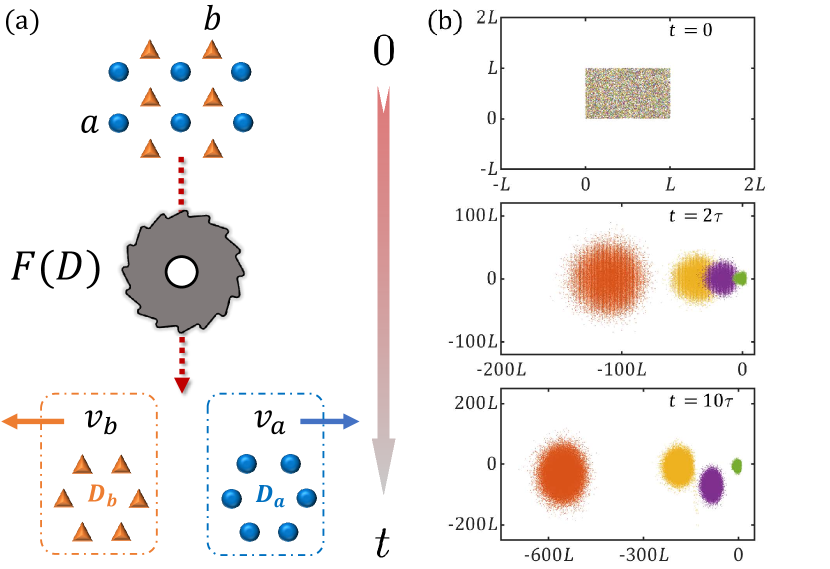
Recent advancements in thermodynamic process control [37, 38, 39, 40, 41, 42] offer new insight into this issue, wherein reverse engineering playing a crucial role in tackling the aforementioned challenge. In this Letter, we employ the Shortcuts to Isothermality (ScI) [40] to revolutionize ratchet-based particle separation. ScI, a notable advancement in nonequilibrium thermodynamics, serves as a transformative tool by facilitating rapid evolution of systems to be controlled towards the thermal equilibrium state of their original Hamiltonians through the auxiliary potentials [40, 41]. Physically, particles experience an effective driving force [43] that depends on their diffusion coefficient $D$, as depicted in Fig. 1(a), leading to the separation of particles with varying $D$. Leveraging the remarkable capabilities offered by ScI, the designed particle evolution in ratchet-based separation is realized, allowing for tractable analytical discussion on typical thermodynamic quantities including particle flux and energy consumption. Moreover, our method can be extended to higher-dimensional cases, as illustrated in Fig. 1(b), enabling efficient separation of various types of particles in distinct directions.

Framework.—As the foundation of this study, we first incorporate ScI into the ratchet-based particle transport schemes. Consider a one-dimensional over-damped Brownian particle coupled to a bath at constant temperature $T$ and driven by a spatial periodic potential $U_{o}\equiv U_{o}(x,\vec{\lambda})$ with period $L$. Here $\vec{\lambda}\equiv\vec{\lambda}(t)$ is a parametric vector with $N\geq 1$ components respectively dependent on time $t$. According to ScI, a designed auxiliary potential $U_{a}^{*}(x,t)$ satisfying [43]

$$\partial_{x}U_{a}^{*}(x,t)=\frac{1}{\beta D^{*}}\frac{\dot{\vec{\lambda}}\cdot\left[\vec{f}_{o}(x,\vec{\lambda})+\vec{j}(\vec{\lambda})\right]}{\rho_{o}(x,\vec{\lambda})}$$ (1)

is exerted on the particle to make its evolution controllable. Here, $D^{*}$ serves as a reference diffusion coefficient but does not necessarily need to be identical to $D$ of the Brownian particle, which is different from the original ScI theory [40]. $\rho_{o}(x,\vec{\lambda})\equiv e^{-\beta U_{o}(x,\vec{\lambda})}/\int_{0}^{L}e^{-\beta U_{o}(x,\vec{\lambda})}dx$ is the normalized equilibrium probability density over one period $0\leq x\leq L$ with $\beta\equiv 1/(k_{\mathrm{B}}T)$ and $k_{\mathrm{B}}$ being the Boltzmann constant, $\vec{f}_{o}(x,\vec{\lambda})\equiv\int_{0}^{x}\vec{\nabla}_{\lambda}\rho_{o}(x^{\prime},\vec{\lambda})dx^{\prime}$, and $\vec{j}(\vec{\lambda})$ is an arbitrary $N$-dimensional vector function. $\vec{\nabla}_{\lambda}\equiv(\partial_{\lambda_{1}},\partial_{\lambda_{2}},\dots,\partial_{\lambda_{N}})$ and $\mathcal{\dot{O}}$ represents the time derivative of an arbitrary physical quantity $\mathcal{O}$.

Associated with the total potential $U^{*}(x,t)=U_{o}(x,\vec{\lambda})+U_{a}^{*}(x,t)$, the evolution of the probability density $\rho(x,t)$ of the particle is governed by the over-damped Fokker-Planck equation [44]

$$\partial_{t}\rho(x,t)=-\partial_{x}\hat{J}_{t}\rho(x,t),$$ (2)

where $\hat{J}_{t}\equiv-D[\beta\partial_{x}U^{*}(x,t)+\partial_{x}]$ is the current operator. Due to the periodicity of the current operator, it suffices to solve Eq. (2) in one period $x\in[0,L]$ [24]. Specifically, we define the reduced probability density $\rho_{s}(x,t)\equiv\sum_{n}\rho(x+nL,t)$ and the reduced probability current $J_{s}(x,t)\equiv\sum_{n}J(x+nL,t)$, where $n\in\mathbb{Z}$ and the probability current reads

$$J(x,t)=\hat{J}_{t}\rho(x,t).$$ (3)

Providing that $\rho(x,t)$ is a normalized solution of Eq. (2), $\rho_{s}(x,t)$ is also a solution which satisfies the periodic condition $\rho_{s}(x,t)=\rho_{s}(x+L,t)$ as well as the conservation condition $\int_{0}^{L}\rho_{s}(x,t)dx=1$. Therefore, the relation between $\rho_{s}(x,t)$ and $J_{s}(x,t)$ is the same as Eq. (3), and the ensemble-averaged velocity of the Brownian particle is defined as $v_{s}(t)\equiv\int_{0}^{L}J_{s}(x,t)dx$.

When all the Brownian particles of interest possess the same diffusion coefficient, it is natural to set $D^{*}=D$. As the result of the original ScI theory, we obtain $\rho_{s}(x,t)=\rho_{o}(x,\vec{\lambda})$ from Eq. (2) and the initial condition $\rho_{s}(x,0)=\rho_{o}(x,0)$. For cases involving multiple particle ensembles with different diffusion coefficients, we need to solve $\rho_{s}(x,t)$ at $D^{*}\neq D$. To carry out further analytical discussion, we assume that the parametric vector $\vec{\lambda}$ changes slowly enough over time, so that $\rho_{s}(x,t)$ can be expanded up to the linear term of $\dot{\vec{\lambda}}$ [45, 46] as follows

$$\rho_{s}(x,t)\approx\rho_{o}(x,\vec{\lambda})+\dot{\vec{\lambda}}\cdot\vec{\psi}(x,t),$$ (4)

where $\vec{\psi}(x,t)$ is a $N$-dimensional vector function to be solved. The equilibrium state is recovered when $\dot{\vec{\lambda}}=0$. Substituting Eq. (4) into Eq. (2) and neglecting the terms containing quadratic time derivative, we obtain

$$\frac{\partial\vec{\psi}(x,t)}{\partial x}+\beta\frac{\partial U_{o}}{\partial x}\vec{\psi}(x,t)=\left(\frac{1}{D}-\frac{1}{D^{*}}\right)\left[\vec{f}_{o}(x,\vec{\lambda})+\vec{C}(t)\right]$$ (5)

with $\vec{C}(t)$ the constant of integration. Solving Eq. (5) with boundary conditions $\vec{\psi}(0,t)=\vec{\psi}(L,t)$ and $\int_{0}^{L}\vec{\psi}(x,t)dx=0$, we find $\vec{C}(t)=-\langle\vec{f}_{o}(x,\vec{\lambda})\rangle_{+}$, where $\langle\cdots\rangle_{\pm}\equiv\int_{0}^{L}e^{\pm\beta U_{o}(x,\vec{\lambda})}\cdots dx/Z_{\pm}(\vec{\lambda})$ and $Z_{\pm}(\vec{\lambda})\equiv\int_{0}^{L}e^{\pm\beta U_{o}(x,\vec{\lambda})}dx$. $\vec{\psi}(x,t)=\vec{\psi}(x,\vec{\lambda})$ is given in [43]. It follows from Eqs. (3) and (5) that

$$J_{s}(x,t)=-\dot{\vec{\lambda}}\cdot\vec{f}(x,\vec{\lambda})+\left(1-\frac{D}{D^{*}}\right)\dot{\vec{\lambda}}\cdot\langle\vec{f}(x,\vec{\lambda})\rangle_{+},$$ (6)

where $\vec{f}(x,\vec{\lambda})\equiv\vec{f}_{o}(x,\vec{\lambda})+\vec{j}(\vec{\lambda})$.

Separating particles with different $D$.—We then investigate the particle flux in steady state. To induce steady-state evolution, we consider that the Brownian particles are periodically driven, namely, $\vec{\lambda}(t)=\vec{\lambda}(t+\tau)$ with the temporal period $\tau$. After enough periods, $\rho_{s}(x,t)$ will enter steady periodic evolution independent of the initial condition [43]. According to Eq. (6), the average reduced probability current over a temporal period $\bar{J}_{s}\equiv\tau^{-1}\int_{t_{0}}^{t_{0}+\tau}J_{s}(x,t)dt$ is specifically obtained as

$$\bar{J}_{s}=\frac{1}{\tau}\left(1-\frac{D}{D^{*}}\right)\Phi_{\mathrm{rev}}-\frac{1}{\tau}\frac{D}{D^{*}}\oint_{I}d\vec{\lambda}\cdot\vec{j}(\vec{\lambda}),$$ (7)

where

$$\Phi_{\mathrm{rev}}\equiv\oint_{I}d\vec{\lambda}\cdot\frac{\int_{0}^{L}e^{\beta U_{o}(x,\vec{\lambda})}\vec{\nabla}_{\lambda}\int_{0}^{x}\rho_{o}(x^{\prime},\vec{\lambda})dx^{\prime}dx}{\int_{0}^{L}e^{\beta U_{o}(x,\vec{\lambda})}dx}$$ (8)

is the integrated flow of reversible ratchets [23, 25] and $I$ is a closed trajectory of $\vec{\lambda}$.

As one of the main results of this Letter, Eq. (7) allows Brownian particles with different $D$ to averagely move at different velocities, thereby enabling their spatial separation. We stress here that i) a spatially asymmetric $U_{o}(x,\vec{\lambda})$ is necessary for generating non-zero $\Phi_{\text{rev}}$ [43]; ii) since $\Phi_{\text{rev}}$ and $\bar{J}_{s}$ are geometric quantities in the $N$-dimensional parametric space that only depend on the geometry of $I$, $N\geq 2$ is required to result in non-zero $\Phi_{\text{rev}}$ and $\bar{J}_{s}$. Obviously, the velocity difference among different particles can be accordingly changed with $\vec{j}(\vec{\lambda})$, $\Phi_{\mathrm{rev}}$, $\tau$, and the setting of $D^{*}$. In particular, when $\vec{j}(\vec{\lambda})=0$, the particles with $D>D^{*}$ and those with $D<D^{*}$ will move in opposite directions, which is consistent with a recent numerical study [28]. In real-world circumstances, different types of particles possess different $D$ due to variations in their shape, size, surface structure, and other characteristics [47, 48, 49, 50]. Therefore, by choosing an appropriate $D^{*}$ to design $U_{a}^{*}(x,t)$ according to Eq. (1), the desired particle separation can be achieved. Noticing $\bar{J}_{s}$ is independent of $x$, it is naturally for us to define the time-ensemble-averaged velocity of the particles as $\bar{v}_{s}\equiv\tau^{-1}\int_{t_{0}}^{t_{0}+\tau}v_{s}(t)dt=\bar{J}_{s}L$. For practical case with $D^{*}\sim 10^{-5}{\rm{cm^{2}/s}},L\sim 0.1{\rm{\mu m}},f=\tau^{-1}\sim 100{\rm{kHz}}$ [28], according to Eq. (7), $\Delta D/D^{*}\sim 1\%$ can result in a velocity difference $\Delta\bar{v}_{s}\sim 0.1\rm{mm/s}$.

Energetic cost for particle separation.—As a thermodynamic task, the energy consumption in driving the particle is another typical quantity that requires significant attention, which can be analyzed with stochastic thermodynamics [51, 52]. When the particles of interest have entered the steady periodic state, their energetics may be captured through the above-solved reduced probability density and reduced probability current. According to the 1st law of thermodynamics, the ensemble-averaged work needed in driving the particle is $W=\Delta E-Q$, where $Q$ is the ensemble-averaged heat absorbed by the particle and $\Delta E$ is the variation of internal energy $E(t)\equiv\int U^{*}(x,t)\rho(x,t)dx$. The total potential $U^{*}(x,t)$ obtained by adding the integral of Eq. (1) on $U_{o}(x,\vec{\lambda})$ is a tilted ratchet potential

$$U^{*}(x,t)=V^{*}(x,t)+\frac{\varepsilon^{*}(t)}{L}x,$$ (9)

where

$$\varepsilon^{*}(t)=\frac{1}{\beta D^{*}}Z_{-}(\vec{\lambda})Z_{+}(\vec{\lambda})\dot{\vec{\lambda}}\cdot\langle\vec{f}(x,\vec{\lambda})\rangle_{+}$$ (10)

is the variation of $U_{a}^{*}(x,t)$ from $x_{0}$ to $x_{0}+L$, and $V^{*}(x,t)\equiv U_{o}(x,\vec{\lambda})+\int_{0}^{x}\partial_{x^{\prime}}U_{a}^{*}(x^{\prime},t)dx^{\prime}-L^{-1}\varepsilon^{*}(t)x$ is a spatial periodic function with period $L$. Here, we have set $U_{a}^{*}(0,t)=0$. Then the internal energy of the particle turns out to be [43]

$$E(t)=\int_{0}^{L}V^{*}(x,t)\rho_{s}(x,t)dx+\frac{\varepsilon^{*}(t)}{L}\langle x\rangle$$ (11)

with $\langle x\rangle\equiv\int_{0}^{L}x\rho_{s}(x,t)dx$ being the ensemble-averaged position of the particle. For periodic driving with $\vec{\lambda}(t_{0})=\vec{\lambda}({t_{0}+\tau})$ and $\dot{\vec{\lambda}}(t_{0})=\dot{\vec{\lambda}}({t_{0}+\tau})$, the variation of the first term in Eq. (11) vanishes in a temporal period. By noticing $\varepsilon^{*}(t_{0})=\varepsilon^{*}(t_{0}+\tau)$ and $\Delta\langle x\rangle=\bar{v}_{s}\tau$, we obtain the internal energy variation as

$$\Delta E=\varepsilon^{*}(t_{0})\bar{J}_{s}\tau=\left(1-\frac{D}{D^{*}}\right)\varepsilon^{*}(t_{0})\Phi_{\mathrm{rev}},$$ (12)

which depends on the initial condition of the driving protocol. Such a initial value dependence diminishes as the particle transport duration increases [43]. Hereafter, unless otherwise stated, we take $\vec{j}(\vec{\lambda})=0$ for simplicity.

Furthermore, the heat current reads $\dot{Q}(t)\equiv\int U^{*}(x,t)\partial_{t}\rho(x,t)dx$ [51, 52], according to which the heat absorption in a temporal period is given as [43]

$$Q=-\int_{t_{0}}^{t_{0}+\tau}dt\dot{\lambda}_{\alpha}\dot{\lambda}_{\beta}G_{\alpha\beta}(\vec{\lambda}).$$ (13)

Here,

$$G_{\alpha\beta}(\vec{\lambda})\equiv \frac{1}{\beta D^{*}}Z_{-}(\vec{\lambda})Z_{+}(\vec{\lambda})\bigg{[}\langle f_{\alpha}(x,\vec{\lambda})f_{\beta}(x,\vec{\lambda})\rangle_{+}$$ (14)

$$-\left(1-\frac{D}{D^{*}}\right)\langle f_{\alpha}(x,\vec{\lambda})\rangle_{+}\langle f_{\beta}(x,\vec{\lambda})\rangle_{+}\bigg{]}$$

is a positive semi-definite matrix [43] with $\alpha,\beta=1,2,\dots,N$, and the Einstein notation has been adopted hereafter.

For a given closed driving trajectory in the parametric space, Cauchy-Schwarz inequality implies that the heat release in Eq. (13) is bounded from below as $-Q\geq\mathcal{L}^{2}/\tau$, where $\mathcal{L}\equiv\int_{0}^{\tau}dt\sqrt{\dot{\lambda}_{\alpha}\dot{\lambda}_{\beta}G_{\alpha\beta}(\vec{\lambda})}$ is the so-called thermodynamic length [53, 54, 55, 41, 46] of the driving loop. Therefore, we have the work cost satisfying $W\geq\Delta E+\mathcal{L}^{2}/\tau$, which, together with Eq. (7), yields the second main result of this Letter

$$W\geq\Delta E+\frac{D^{*}\mathcal{L}^{2}\bar{J}_{s}}{\left(D^{*}-D\right)\Phi_{\mathrm{rev}}},$$ (15)

where the equal sign is saturated when the integrand of $\mathcal{L}$ is a time-independent constant [54, 55], namely,

$$\tau\sqrt{\dot{\lambda}_{\alpha}\dot{\lambda}_{\beta}G_{\alpha\beta}(\vec{\lambda})}-\mathcal{L}=0.$$ (16)

Equation (15) indicates that the minimal extra energetic cost ($W_{\rm{ex}}\equiv W-\Delta E$ which is exactly the heat dissipation) for particle separation is directly proportional to the particle flow, namely, faster particle separation (shorter $\tau$) requires more work consumption for given $\Delta E$. In the quasi-static limit ($\bar{J}_{s}\rightarrow 0$), one has $W\rightarrow\Delta E$. Moreover, for given parametric loop and $\tau$ (which correspond to a certain average particle velocity), Eq. (16) determines the optimal driving protocol associated with the minimal $W_{\rm{ex}}$.

Figure 2: (a) One period of the original periodic potential $U_{o}(x,\vec{\lambda})$. (b) The trajectory of the driving protocol $\vec{\lambda}(t)$ is a anticlockwise circle with radius $R$. (c) The tilted total potential $U^{*}(x,t)$ and the periodic steady reduced probability density $\rho_{s}(x,t)$ at a certain time.

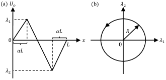
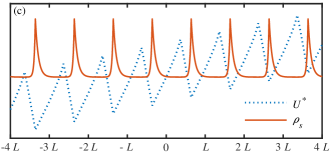
Example.—We illustrate our general theoretical framework with an example, where $U_{o}$ is specific as the sawtooth potential which, shown in Fig. 2(a), is one of the most common ratchet potential. The height $\lambda_{1}$ and depth $\lambda_{2}$ of the potential serve as time-dependent parameters, i.e., $\vec{\lambda}=(\lambda_{1},\lambda_{2})$. According to Eq. (7), $U_{o}(x,\vec{\lambda})$ relates to the average particle probability current via $\Phi_{\text{rev}}$. Hence, the shape of the potential as well as the geometry of the driving loop in the parametric space can be optimized to induce large particle current. After comprehensive evaluations [43], we find that it is favorable to set $\alpha=0.36$ and the driving loop as a circle in Fig. 2(b). Fig. 2(c) is a snapshot of the total potential $U^{*}(x,t)$ and the steady reduced probability density $\rho_{s}(x,t)$ respectively according to Eq. (9) and Eq. (4). $\rho_{s}(x,t)$ and the gradient of $U^{*}(x,t)$ are both periodic in infinite space. The dynamic equation of the over-damped Brownian particles reads $\dot{x}=-\beta D\partial_{x}U^{*}(x,t)+\sqrt{2D}\xi(t)$ [56], where the normalized Gaussian white noise $\xi(t)$ satisfies $\langle\xi(t)\rangle=0$ and $\langle\xi(t)\xi(t^{\prime})\rangle=\delta(t-t^{\prime})$. We simulate the movement of $10^{5}$ particles by solving this equation with Euler algorithm [43]. The quantities in the simulation are nondimensionalized by $L$, $\beta^{-1}$ and $D^{*}$. $\mathcal{\tilde{O}}$ denotes the dimensionless $\mathcal{O}$. For example, $\widetilde{v_{s}}\equiv D^{*-1}Lv_{s}$.

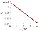
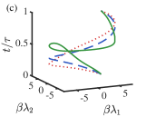
We first validate the effectiveness of Eq. (7). The time-ensemble-averaged velocities $\widetilde{\bar{v}_{s}}$ of particles for different diffusion coefficients are plotted in Fig. 3(a) with $\tilde{\tau}\equiv D^{*}L^{-2}\tau=20$. The simulation data (red circles) are in good alignment with the theoretical prediction (solid line). In Fig. 3(b), we illustrate $\widetilde{\bar{v}_{s}}$ as a function of $\tilde{\tau}$ for $D/D^{*}=2$ (circles) and $D/D^{*}=1/2$ (squares). As expected, the simulated marks coincide well with the theoretical lines in the slow-driving regime ($\tilde{\tau}\gg 1$). Furthermore, the energetics of the particle can be consistently obtained in simulations. By definition [51], the absorbed heat and the input work of a particle from $t$ to $t+\Delta t$ are respectively $\Delta q=U^{*}(x+\Delta x,t+\Delta t)-U^{*}(x,t+\Delta t)$ and $\Delta w=U^{*}(x,t+\Delta t)-U^{*}(x,t)$, where $\Delta x$ is the position variation within $\Delta t$. We now test Eq. (15) with three different protocols $f(s)$ associated with the driving loop (Fig. 2(b)) $\lambda_{1}=R\cos[2\pi f(s)+\theta_{0}]$, $\lambda_{2}=R\sin[2\pi f(s)+\theta_{0}]$, where $s\equiv t/\tau$ and $\theta_{0}=\pi/6$. The time-dependent paths are demonstrated in Fig. 3(c): Path-I: $f_{1}(s)=\sum_{i=1}^{i=3}a_{i}s^{i}$ with $a_{1}=2,a_{2}=-3,a_{3}=2$ (red dotted line) [57], Path-II: $f_{2}(s)=s$ (blue dashed line), and Path-III: the optimal protocol (green solid line) obtained numerically from Eq. (16) [43]. The corresponding extra work $W_{\rm{ex}}$ are illustrated in Fig. 3(d), where the dotted and dashed lines (plotted with Eq. (13)) and the solid line (the lower bound of Eq. (15)) agree well with the numerical results (marks). Clearly, the optimal protocol [58] indeed lead to lower $W_{\rm{ex}}$ (green circles) than those associated with Path-I (red triangles) and Path-II (blue squares).

Figure 3: (a) The time-ensemble-averaged velocity $\widetilde{\bar{v}_{s}}$ as a function of $D/D^{*}$ with $\tilde{\tau}=20$. (b) $\widetilde{\bar{v}_{s}}$ as a function of $\tilde{\tau}$ for $D/D^{*}=2$ (circles and dashed line) and $D/D^{*}=1/2$ (squares and dotted line). (c) Three different driving protocols, i.e., path-I (red dotted line), path-II (blue dashed line), and path-III (green solid line). (d) The extra energetic cost $W_{\rm{ex}}$ as a function of $\tilde{\tau}$ with $D/D^{*}=2$. The three data series from top to bottom respectively correspond to path-I, path-II and path-III. The marks and lines in (a)(b)(d) are simulation results and analytical predictions, respectively. In the simulations, characteristic quantities are set as $L=1$, $\beta=1$, $D^{*}=1$, and $\beta R=7$, the number of particles is $N=10^{5}$ and the time step is $\Delta\tilde{t}=10^{-4}$.

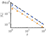
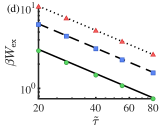
Finally, we would like to make three remarks here. First, although generated under path-I, the results in Fig. 3(a) and (b) are independent of the specific choice of driving protocol $f(s)$ since the time-ensemble-averaged velocity is a geometric quantity (dynamic-independent) in the parametric space. Second, in the slow-driving regime (also known as long-time regime), the $1/\tau$-scaling exhibited by the particle flux (Fig. 3(b)) and energetic cost (Fig. 3(d)) is a typical manifestation of finite-time irreversibility [59, 40, 60, 61, 41, 46]. Third, for practical purposes, the developed ScI-ratchet can be straightforwardly generalized to higher-dimensional space to simultaneously separate more kinds of particles, as demonstrated in Fig. 1(b). Detailed information of this case is given in [43].

Summary.— We develop a universal framework that integrates thermodynamic process engineering into ratchet-based particle transport, enabling directional separation of Brownian particles with different diffusion coefficients. By utilizing ScI, which allows controlled evolution of particles towards an thermal equilibrium distribution, we provide analytical expressions for key quantities in the particle separation process, such as particle flux, heat dissipation, and required work. With the thermodynamic geometry theory, we determine the optimal separation protocol that minimize the energetic consumption while maintaining a given particle flux. We also demonstrate the extensibility of this approach in higher-dimensional space.

Currently, the combination of thermodynamic geometry and thermodynamic process control in optimizing practical thermodynamic tasks, such as heat engine optimization [62, 63, 64] and information erasure [46, 65], has attracted widespread research interest. Our work provides new application scenarios for this area and lays the foundation for further incorporation of thermodynamic process engineering into ratchet-based particle separation. In relation to this, it is interesting to investigate ScI-assisted chiral separation [66, 67, 68] and mass separation [12, 69, 70, 71]. Our proposed Brownian particle separation method and the corresponding theoretical predictions can be experimental realized and tested in some state-of-art platforms [72, 73].

Acknowledgments.— Y. H. Ma thanks the National Natural Science Foundation of China for support under grant No. 12305037 and the Fundamental Research Funds for the Central Universities under grant No. 2023NTST017. Z. C. Tu thanks the National Natural Science Foundation of China for support under grant No. 11975050.

References

- Harnisch and Schröder [2009] F. Harnisch and U. Schröder, Selectivity versus mobility: Separation of anode and cathode in microbial bioelectrochemical systems, ChemSusChem 2, 921 (2009).
- Xie et al. [2014] F. Xie, T. A. Zhang, D. Dreisinger, and F. Doyle, A critical review on solvent extraction of rare earths from aqueous solutions, Minerals Engineering 56, 10 (2014).
- Sholl and Lively [2016] D. S. Sholl and R. P. Lively, Seven chemical separations to change the world, Nature 532, 435 (2016).
- Makanyire et al. [2016] T. Makanyire, S. Sanchez-Segado, and A. Jha, Separation and recovery of critical metal ions using ionic liquids, Advances in Manufacturing 4, 33 (2016).
- Yang et al. [2018] S. Yang, F. Zhang, H. Ding, P. He, and H. Zhou, Lithium metal extraction from seawater, Joule 2, 1648 (2018).
- Nouri and Guan [2021] R. Nouri and W. Guan, Nanofluidic charged-coupled devices for controlled DNA transport and separation, Nanotechnology 32, 345501 (2021).
- Mei et al. [2022] T. Mei, H. Zhang, and K. Xiao, Bioinspired artificial ion pumps, ACS Nano 16, 13323 (2022).
- Zamboulis et al. [2011] D. Zamboulis, E. N. Peleka, N. K. Lazaridis, and K. A. Matis, Metal ion separation and recovery from environmental sources using various flotation and sorption techniques, Journal of Chemical Technology & Biotechnology 86, 335 (2011).
- Reguera et al. [2012] D. Reguera, A. Luque, P. S. Burada, G. Schmid, J. M. Rubí, and P. Hänggi, Entropic splitter for particle separation, Physical Review Letters 108, 020604 (2012).
- Zhang et al. [2020] X. Zhang, K. Zuo, X. Zhang, C. Zhang, and P. Liang, Selective ion separation by capacitive deionization (CDI) based technologies: a state-of-the-art review, Environmental Science: Water Research & Technology 6, 243 (2020).
- Yoon et al. [2019] H. Yoon, J. Lee, S. Kim, and J. Yoon, Review of concepts and applications of electrochemical ion separation (EIONS) process, Separation and Purification Technology 215, 190 (2019).
- Słapik et al. [2019] A. Słapik, J. Łuczka, P. Hänggi, and J. Spiechowicz, Tunable mass separation via negative mobility, Physical Review Letters 122, 070602 (2019).
- Marbach and Bocquet [2017] S. Marbach and L. Bocquet, Active sieving across driven nanopores for tunable selectivity, The Journal of Chemical Physics 147, 154701 (2017).
- Park et al. [2017] H. B. Park, J. Kamcev, L. M. Robeson, M. Elimelech, and B. D. Freeman, Maximizing the right stuff: The trade-off between membrane permeability and selectivity, Science 356, eaab0530 (2017).
- Goh et al. [2018] P. S. Goh, W. J. Lau, M. H. D. Othman, and A. F. Ismail, Membrane fouling in desalination and its mitigation strategies, Desalination 425, 130 (2018).
- Tang and Bruening [2020] C. Tang and M. L. Bruening, Ion separations with membranes, Journal of Polymer Science 58, 2831 (2020).
- Epsztein et al. [2020] R. Epsztein, R. M. DuChanois, C. L. Ritt, A. Noy, and M. Elimelech, Towards single-species selectivity of membranes with subnanometre pores, Nature Nanotechnology 15, 426 (2020).
- Rousselet et al. [1994] J. Rousselet, L. Salome, A. Ajdari, and J. Prostt, Directional motion of brownian particles induced by a periodic asymmetric potential, Nature 370, 446 (1994).
- Faucheux and Libchaber [1995] L. P. Faucheux and A. Libchaber, Selection of brownian particles, Journal of the Chemical Society, Faraday Transactions 91, 3163 (1995).
- Bader et al. [1999] J. S. Bader, R. W. Hammond, S. A. Henck, M. W. Deem, G. A. McDermott, J. M. Bustillo, J. W. Simpson, G. T. Mulhern, and J. M. Rothberg, DNA transport by a micromachined brownian ratchet device, Proceedings of the National Academy of Sciences 96, 13165 (1999).
- Matthias and Müller [2003] S. Matthias and F. Müller, Asymmetric pores in a silicon membrane acting as massively parallel brownian ratchets, Nature 424, 53 (2003).
- Doering [1995] C. R. Doering, Randomly rattled ratchets, Il Nuovo Cimento D 17, 685 (1995).
- Parrondo et al. [1998] J. M. R. Parrondo, J. M. Blanco, F. J. Cao, and R. Brito, Efficiency of brownian motors, Europhysics Letters 43, 248 (1998).
- Reimann [2002] P. Reimann, Brownian motors: noisy transport far from equilibrium, Physics Reports 361, 57 (2002).
- Parrondo and de Cisneros [2002] J. Parrondo and B. de Cisneros, Energetics of brownian motors: a review, Applied Physics A 75, 179 (2002).
- Lau and Kedem [2020] B. Lau and O. Kedem, Electron ratchets: State of the field and future challenges, The Journal of Chemical Physics 152, 200901 (2020).
- Nicollier et al. [2021] P. Nicollier, C. Schwemmer, F. Ruggeri, D. Widmer, X. Ma, and A. W. Knoll, Nanometer-scale-resolution multichannel separation of spherical particles in a rocking ratchet with increasing barrier heights, Physical Review Applied 15, 034006 (2021).
- Herman et al. [2023] A. Herman, J. W. Ager, S. Ardo, and G. Segev, Ratchet-based ion pumps for selective ion separations, PRX Energy 2, 023001 (2023).
- Rozenbaum [2008] V. M. Rozenbaum, High-temperature brownian motors: Deterministic and stochastic fluctuations of a periodic potential, JETP Letters 88, 342 (2008).
- Chr. Germs et al. [2013] W. Chr. Germs, E. M. Roeling, L. J. van IJzendoorn, R. A. J. Janssen, and M. Kemerink, Diffusion enhancement in on/off ratchets, Applied Physics Letters 102, 073104 (2013).
- Kedem et al. [2017] O. Kedem, B. Lau, and E. A. Weiss, How to drive a flashing electron ratchet to maximize current, Nano Letters 17, 5848 (2017).
- Kanada et al. [2018] R. Kanada, R. Shinagawa, and K. Sasaki, Diffusion enhancement of brownian motors revealed by a solvable model, Physical Review E 98, 062110 (2018).
- Fane et al. [1987] A. G. Fane, R. Schofield, and C. J. D. Fell, The efficient use of energy in membrane distillation, Desalination 64, 231 (1987).
- Tsirlin et al. [2002] A. M. Tsirlin, V. Kazakov, and D. V. Zubov, Finite-time thermodynamics: Limiting possibilities of irreversible separation processes, The Journal of Physical Chemistry A 106, 10926 (2002).
- Huang et al. [2010] Y. Huang, R. W. Baker, and L. M. Vane, Low-energy distillation-membrane separation process, Industrial & Engineering Chemistry Research 49, 3760 (2010).
- Chen et al. [2023] J.-F. Chen, R.-X. Zhai, C. Sun, and H. Dong, Geodesic lower bound of the energy consumption to achieve membrane separation within finite time, PRX Energy 2, 033003 (2023).
- Guéry-Odelin et al. [2019] D. Guéry-Odelin, A. Ruschhaupt, A. Kiely, E. Torrontegui, S. Martínez-Garaot, and J. Muga, Shortcuts to adiabaticity: Concepts, methods, and applications, Reviews of Modern Physics 91, 045001 (2019).
- Nakamura et al. [2020] K. Nakamura, J. Matrasulov, and Y. Izumida, Fast-forward approach to stochastic heat engine, Physical Review E 102, 012129 (2020).
- Guéry-Odelin et al. [2023] D. Guéry-Odelin, C. Jarzynski, C. A. Plata, A. Prados, and E. Trizac, Driving rapidly while remaining in control: classical shortcuts from hamiltonian to stochastic dynamics, Reports on Progress in Physics 86, 035902 (2023).
- Li et al. [2017] G. Li, H. T. Quan, and Z. C. Tu, Shortcuts to isothermality and nonequilibrium work relations, Physical Review E 96, 012144 (2017).
- Li et al. [2022] G. Li, J.-F. Chen, C. Sun, and H. Dong, Geodesic path for the minimal energy cost in shortcuts to isothermality, Physical Review Letters 128, 230603 (2022).
- Li and Tu [2023] G. Li and Z. C. Tu, Nonequilibrium work relations meet engineered thermodynamic control: A perspective for nonequilibrium measurements, Europhysics Letters 142, 61001 (2023).
- [43] See supplemental materials for analytical derivations regarding framework (Sec. I) and energetics (Sec. II). The simulation details are given in Sec. III.
- Reichl [2016] L. E. Reichl, A modern course in statistical physics (John Wiley & Sons, 2016).
- Cavina et al. [2017] V. Cavina, A. Mari, and V. Giovannetti, Slow dynamics and thermodynamics of open quantum systems, Physical review letters 119, 050601 (2017).
- Ma et al. [2022] Y.-H. Ma, J.-F. Chen, C. Sun, and H. Dong, Minimal energy cost to initialize a bit with tolerable error, Physical Review E 106, 034112 (2022).
- Mun et al. [2014] E. A. Mun, C. Hannell, S. E. Rogers, P. Hole, A. C. Williams, and V. V. Khutoryanskiy, On the role of specific interactions in the diffusion of nanoparticles in aqueous polymer solutions, Langmuir 30, 308 (2014).
- Chan et al. [2015] T. C. Chan, H. T. Li, and K. Y. Li, Effects of shapes of solute molecules on diffusion: A study of dependences on solute size, solvent, and temperature, The Journal of Physical Chemistry B 119, 15718 (2015).
- Iwahashi and Kasahara [2007] M. Iwahashi and Y. Kasahara, Effects of molecular size and structure on self-diffusion coefficient and viscosity for saturated hydrocarbons having six carbon atoms, Journal of Oleo Science 56, 443 (2007).
- Marrero and Mason [2009] T. R. Marrero and E. A. Mason, Gaseous diffusion coefficients, Journal of Physical and Chemical Reference Data 1, 3 (2009).
- Sekimoto [2010] K. Sekimoto, Stochastic Energetics (Springer, 2010).
- Seifert [2012] U. Seifert, Stochastic thermodynamics, fluctuation theorems and molecular machines, Reports on Progress in Physics 75, 126001 (2012).
- Salamon and Berry [1983] P. Salamon and R. S. Berry, Thermodynamic length and dissipated availability, Physical Review Letters 51, 1127 (1983).
- Crooks [2007] G. E. Crooks, Measuring thermodynamic length, Physical Review Letters 99, 100602 (2007).
- Sivak and Crooks [2012] D. A. Sivak and G. E. Crooks, Thermodynamic metrics and optimal paths, Physical review letters 108, 190602 (2012).
- Zwanzig [2001] R. Zwanzig, Nonequilibrium Statistical Mechanics (Oxford University Press, 2001).
- [57] In fact, only a free parameter exsits in this protocol, since and are imposed to ensure the continuity of and its first derivative along the driving loop.
- [58] The presented optimal path associated with the minimum on a given trajectory in the parametric space. There may exist different trajectories leading to the same particle flux but have different energy cost. Determining the optimal trajectory and the corresponding driving protocol is an open question for achieving globally optimal control in both geometric and dynamic regimes.
- Martínez et al. [2016] I. A. Martínez, É. Roldán, L. Dinis, D. Petrov, J. M. Parrondo, and R. A. Rica, Brownian carnot engine, Nature physics 12, 67 (2016).
- Ma et al. [2020] Y.-H. Ma, R.-X. Zhai, J. Chen, C. Sun, and H. Dong, Experimental test of the 1/-scaling entropy generation in finite-time thermodynamics, Physical Review Letters 125, 210601 (2020).
- Yuan et al. [2022] H. Yuan, Y.-H. Ma, and C. P. Sun, Optimizing thermodynamic cycles with two finite-sized reservoirs, Physical Review E 105, L022101 (2022).
- Ma et al. [2018] Y.-H. Ma, D. Xu, H. Dong, and C.-P. Sun, Optimal operating protocol to achieve efficiency at maximum power of heat engines, Physical Review E 98, 022133 (2018).
- Frim and DeWeese [2022] A. G. Frim and M. R. DeWeese, Geometric bound on the efficiency of irreversible thermodynamic cycles, Physical Review Letters 128, 230601 (2022).
- Zhao et al. [2022] X.-H. Zhao, Z.-N. Gong, and Z. Tu, Low-dissipation engines: Microscopic construction via shortcuts to adiabaticity and isothermality, the optimal relation between power and efficiency, Physical Review E 106, 064117 (2022).
- Rolandi et al. [2023] A. Rolandi, P. Abiuso, and M. Perarnau-Llobet, Collective advantages in finite-time thermodynamics, Physical Review Letters 131, 210401 (2023).
- Marcos et al. [2009] Marcos, H. C. Fu, T. R. Powers, and R. Stocker, Separation of microscale chiral objects by shear flow, Physical Review Letters 102, 158103 (2009).
- Bechinger et al. [2016] C. Bechinger, R. Di Leonardo, H. Lowen, C. Reichhardt, G. Volpe, and G. Volpe, Active particles in complex and crowded environments, Reviews of Modern Physics 88, 045006 (2016).
- Xu et al. [2022] G.-h. Xu, T.-C. Li, and B.-q. Ai, Sorting of chiral active particles by a spiral shaped obstacle, Physica A: Statistical Mechanics and its Applications 608, 128247 (2022).
- Khatri and Burada [2021] N. Khatri and P. S. Burada, Mass separation in an asymmetric channel, Physical Review E 104, 044109 (2021).
- Khatri and Kapral [2023] N. Khatri and R. Kapral, Inertial effects on rectification and diffusion of active brownian particles in an asymmetric channel, The Journal of Chemical Physics 158, 124903 (2023).
- Gupta and Burada [2023] A. Gupta and P. S. Burada, Separation of interacting active particles in an asymmetric channel, Physical Review E 108, 034605 (2023).
- Albay et al. [2019] J. A. C. Albay, S. R. Wulaningrum, C. Kwon, P.-Y. Lai, and Y. Jun, Thermodynamic cost of a shortcuts-to-isothermal transport of a brownian particle, Physical Review Research 1, 033122 (2019).
- Albay et al. [2020] J. A. C. Albay, P.-Y. Lai, and Y. Jun, Realization of finite-rate isothermal compression and expansion using optical feedback trap, Applied Physics Letters 116, 103706 (2020).