Temporal Entropy Evolution in Stochastic and Delayed Dynamics

Abstract

We review the behaviour of the Gibbs’ and conditional entropies in deterministic and stochastic systems with the added twist of a formulation appropriate for a stochastically perturbed system with delayed dynamics. The underlying question driving these investigations: “Is the origin of the universally observed unidirectionality of time in our universe connected to the behaviour of entropy?”

We focus on temporal entropic behaviour with a review of previous results in deterministic and stochastic systems. Our emphasis is on the temporal behaviour of the Gibbs’ and conditional entropies as they give equilibrium results in concordance with experimental findings. In invertible deterministic systems both entropies are temporally constant as has been well known for decades. The addition of stochastic perturbations (Wiener process) leads to an indeterminate (either increasing or decreasing) behaviour of the Gibbs’ entropy, but the conditional entropy monotonically approaches equilibrium with increasing time. The presence of delays in the dynamics, whether stochastically perturbed or not, leads to situations in which the Gibbs’ and conditional entropies evolution can be oscillatory and not monotone, and may not approach equilibrium.

Keywords: density evolution, conditional entropy, Gibbs’ entropy, Ornstein-Uhlenbeck process, Gaussian process

1 Introduction

In this review, we focus on the temporal behaviour of the Gibbs’ and conditional entropies in dynamical and semi-dynamical systems with both stochastic perturbations as well as delayed dynamics, building on and extending the recent results of Mackey and Tyran-Kamińska (2021) as well as older results (Mackey and Tyran-Kamińska, 2006a, b)

The outline of the paper is as follows. Section 2 defines the the Gibbs’ and conditional entropies, while Section 3 shows that these entropies are constant in time in invertible deterministic system (e.g. a system of ordinary differential equations). Section 4 introduces the dynamic concept of asymptotic stability,, and two main results connecting the convergence of the conditional entropy with asymptotic stability (Theorem 4.1), and the existence of unique stationary densities with the convergence of the conditional entropy (Theorem 4.2). Section 5 considers the stochastic extension where a system of ordinary equations is perturbed by Gaussian white noise (thus becoming non-invertible) and gives general results showing that in this stochastic case asymptotic stability holds. In this section we give examples of the effects of noise on the behaviour of the Gibbs and conditional entropy. Following this we turn to an examination of the effects of delays in the dynamics on the evolution of the conditional entropy in Section 6. We conclude with a short discussion.

2 Entropies: Gibbs and conditional.

Two types of entropies are considered here. The first is the Gibbs’ entropy, which is an extension of the equilibrium entropy introduced by Gibbs (1962) to a time dependent situation. This has been considered by a number of authors, namely Ruelle (1996, 2003), Nicolis and Daems (1998), Daems and Nicolis (1999) and Bag (2002a, b, 2003).

In his seminal work Gibbs (1962), assuming the existence of a system steady state density $f_{*}$ on the phase space ${X}$, introduced the concept of the index of probability given by $(-\ln f_{*}(x))$ where “$\ln$” denotes the natural logarithm. He then identified the entropy in a steady state situation with the average of the index of probability

$$H_{G}(f_{*})=-\int_{X}f_{*}(x)\ln f_{*}(x)\,dx.$$ (2.1)

This is called the equilibrium or steady state Gibbs’ entropy.

The Gibbs’ equilibrium entropy definition Eq. 2.1 has repeatedly proven to yield correct results when applied to a variety of equilibrium situations (Mayer and Mayer, 1940; Reichl, 1980; Ter Haar, 1995; Kittel, 2004; Penrose, 2005; Hill, 2013) and this is why it is the gold standard for equilibrium computations in statistical mechanics and thermodynamics. Thus it makes total sense to identify the equilibrium Gibbs’ entropy ${H_{G}(f_{*})}$ with the equilibrium thermodynamic entropy.

The question of how a time dependent non-equilibrium entropy should be defined has interested investigators for some time, and specifically the question of whether the Gibbs’ entropy $H_{G}(f)$ should be extended to a time dependent situation has occupied many researchers. Various aspects of this question have been considered (Daems and Nicolis, 1999; Ruelle, 1996, 1997, 2003, 2004) and if the definition of the steady state Gibbs’ entropy is extended to time dependent (non-equilibrium) situations then the time dependent Gibbs’ entropy of a density $f(x,t)$ is defined by

$$H_{G}(f)=-\int_{X}f(x,t)\ln f(x,t)\,dx.$$ (2.2)

A second type of entropy, the conditional entropy, is a generalization of the Gibbs’ entropy. Convergence properties of the conditional entropy have been extensively studied because entropy methods have been known for some time to be useful for problems involving questions related to convergence of solutions in partial differential equations (Loskot and Rudnicki, 1991; Abbondandolo, 1999; Toscani and Villani, 2000; Arnold et al., 2001; Qian, 2001; Qian et al., 2002). Explicitly, we define the conditional entropy as (Lasota and Mackey, 1994)

$$H_{c}(f|f_{*})=-\int_{X}f(x,t)\ln\dfrac{f(x,t)}{f_{*}(x)}dx.$$ (2.3)

This is also known as the Kullback-Leibler or relative entropy (Loskot and Rudnicki, 1991), or the relative Boltzmann entropy (Eu, 1997), and has been related to the thermodynamic free energy (Qian, 2002).

3 Gibbs’ and conditional entropy in invertible deterministic systems

To set the stage let $(X,\mathcal{B},\mu)$ be a $\sigma$-finite measure space. Further, let $\{P^{t}\}_{t\geq 0}$ be a semigroup of Markov operators on $L^{1}(X,\mu)$, i.e. $P^{t}f\geq 0$ for $f\geq 0$, $\int P^{t}f(x)\,\mu(dx)=\int f(x)\,\mu(dx)$, and $P^{t+s}f=P^{t}(P^{s}f)$. If the group property holds for $t,s\in\mathbb{R}$, then we say that $P$ is invertible, while if it holds only for $t,s\in\mathbb{R}^{+}$ we say that $P$ is non-invertible. We denote the corresponding set of densities by $\mathcal{D}(X,\mu)$, or $\mathcal{D}$ when there will be no ambiguity, so $f\in\mathcal{D}$ means $f\geq 0$ and $||f||_{1}=\int_{X}f(x)\,\mu(dx)=1$. A density $f_{*}$ is called a stationary density of $P^{t}$ if $P^{t}f_{*}=f_{*}$ for all $t$.

In this section we briefly consider entropy behaviour in situations where the dynamics are invertible in the sense that they can be run forward or backward in time without ambiguity. To make this clearer, consider a phase space $X$ and a dynamics $S_{t}:X\to X$. For every initial point $x^{0}$, the sequence of successive points $S_{t}(x^{0})$, considered as a function of time $t$, is called a trajectory. In the phase space $X$, if the trajectory $S_{t}(x^{0})$ is nonintersecting with itself, or intersecting but periodic, then at any given final time $t_{f}$ such that $x^{f}=S_{t_{f}}(x^{0})$ we could change the sign of time by replacing $t\rightarrow(-t)$, and run the trajectory backward using $x^{f}$ as a new initial point in $X$. Then our new trajectory $S_{-t}(x^{f})$ would arrive precisely back at $x^{0}$ after a time $t_{f}$ had elapsed: $x^{0}=S_{-t_{f}}(x^{f})$. Thus in this case we have a dynamics that may be reversed in time completely unambiguously.

We formalize this by introducing the concept of a dynamical system $\{S_{t}\}_{t\in\mathbb{R}}$, which is simply any group of transformations $S_{t}:X\rightarrow X$ having the two properties: 1. $S_{0}(x)=x$; and 2. $S_{t}(S_{t^{\prime}}(x))=S_{t+t^{\prime}}(x)$ for $t,t^{\prime}\in\mathbb{R}$ or $\mathbb{Z}$. Since, from the definition, for any $t\in\mathbb{R}$, we have $S_{t}(S_{-t}(x))=x=S_{-t}(S_{t}(x))$, it is clear that dynamical systems are invertible in the sense discussed above since they may be run either forward or backward in time. Systems of ordinary differential equations are examples of dynamical systems.

The first result is very general, and shows that the conditional entropy of any invertible system is constant and uniquely determined by the method of system preparation. Thus

Theorem 3.1.

(Mackey, 2011, Thm. 3.2) If $P^{t}$ is an invertible Markov operator and has a stationary density $f_{*}$, then the conditional entropy is constant and equal to the value determined by $f_{*}$ and the choice of the initial density $f_{0}$ for all time $t$. That is,

$$H_{c}(P^{t}f_{0}|f_{*})\equiv H_{c}(f_{0}|f_{*})$$

for all $t$.

In the case where we are considering a deterministic dynamics $S_{t}:{\cal X}\to{\cal X}$ where ${\cal X}\subset X$, then the corresponding Markov operator is also known as the Frobenius Perron operator (Lasota and Mackey, 1994), and is given explicitly by

$$P^{t}f_{0}(x)=f_{0}(S_{-t}(x))|J^{-t}(x)|$$

where $J^{-t}(x)$ denotes the Jacobian of $S_{-t}(x)$. A simple calculation shows

$$H_{c}(P^{t}f_{0}|f_{*}) = -\int_{\cal X}P^{t}f_{0}(x)\log\left[\dfrac{P^{t}f_{0}(x)}{f_{*}(x)}\right]\,dx$$

$$= -\int_{\cal X}f_{0}(S_{-t}(x))|J^{-t}(x)|\log\left[\dfrac{f_{0}(S_{-t}(x))}{f_{*}(S_{-t}(x))}\right]\,dx$$

$$= -\int_{\cal X}f_{0}(y)\log\left[\dfrac{f_{0}(y)}{f_{*}(y)}\right]\,dy$$

$$\equiv H_{c}(f_{0}|f_{*})$$

as expected from Theorem 3.1.

More specifically, if the dynamics corresponding to our invertible Markov operator are described by the system of ordinary differential equations

$$\dfrac{dx_{i}}{dt}=F_{i}(x)\qquad i=1,\ldots,d$$ (3.1)

operating in a region of $\mathbb{R}^{d}$ with initial conditions $x_{i}(0)=x_{i,0}$, then (Lasota and Mackey, 1994) the evolution of $f(x,t)\equiv P^{t}f_{0}(x)$ is governed by the generalized Liouville equation

$$\frac{\partial f}{\partial t}=-\sum_{i}\frac{\partial(fF_{i})}{\partial x_{i}}.$$ (3.2)

The corresponding stationary density $f_{*}$ is given by the solution of

$$\sum_{i}\frac{\partial(f_{*}F_{i})}{\partial x_{i}}=0.$$

Note that the uniform density $f_{*}\equiv 1$, meaning that the flow defined by Eq. 3.1 preserves the Lebesque measure, is a stationary density of Eq. 3.2 if and only if

$$\sum_{i}\frac{\partial F_{i}}{\partial x_{i}}=0.$$

In particular, for the system of ordinary differential equations (3.1) whose density evolves according to the Liouville equation (3.2) we can assert that the conditional entropy of the density $P^{t}f_{0}$ with respect to the stationary density $f_{*}$ will be constant for all time and will have the value determined by the initial density $f_{0}$ with which the system is prepared. This result can also be proved directly by noting that from the definition of the conditional entropy we may write

$$H_{c}(f|f_{*})=-\int_{\mathbb{R}^{d}}f(x)\left[\log\left(\frac{f}{f_{*}}\right)+\frac{f_{*}}{f}-1\right]\,dx$$

when the stationary density is $f_{*}$. Differentiating with respect to time gives

$$\frac{dH_{c}}{dt}=-\int_{\mathbb{R}^{d}}\frac{df}{dt}\log\left[\frac{f}{f_{*}}\right]\,dx$$

or, after substituting from (3.2) for $(\partial f/\partial t)$, and integrating by parts under the assumption that $f$ has compact support,

$$\frac{dH_{c}}{dt}=\int_{\mathbb{R}^{d}}\frac{f}{f_{*}}\sum_{i}\frac{\partial(f_{*}F_{i})}{\partial x_{i}}\,dx.$$

However, since $f_{*}$ is a stationary density of $P^{t}$, it is clear from (3.2) that

$$\frac{dH_{c}}{dt}=0,$$ (3.3)

and we conclude that the conditional entropy $H_{c}(P^{t}f_{0}|f_{*})$ does not change from its initial value when the dynamics evolve in this manner. It is obvious that this conclusion also holds for the Gibbs’ entropy.

4 Asymptotic stability and entropy behaviour

We call a semigroup of Markov operators $P^{t}$ on $L^{1}(X,\mu)$ asymptotically stable if there is a density $f_{*}$ such that $P^{t}f_{*}=f_{*}$ for all $t>0$ and for all densities $f$

$$\lim_{t\to\infty}||P^{t}f-f_{*}||_{1}=0.$$

Theorem 4.1.

(Mackey, 2011, Thm. 7.7) Let $P^{t}$ be a semigroup of Markov operators on $L^{1}(X,\mu)$ and $f_{*}$ be a positive density. If

$$\lim_{t\to\infty}H_{c}(P^{t}f|f_{*})=0$$ (4.1)

for a density $f$ then

$$\lim_{t\to\infty}||P^{t}f-f_{*}||_{1}=0.$$ (4.2)

Conversely, if $P^{t}f_{*}=f_{*}$ for all $t\geq 0$ and Condition 4.2 holds for all $f$ with $H_{c}(f|f_{*})>-\infty$, then Condition 4.1 holds as well.

Thus from this theorem asymptotic stability is necessary and sufficient for the convergence of $H_{c}$ to zero. Our next result draws a connection between the existence of a unique stationary density $f_{*}$ of $P^{t}$ and the convergence of the conditional entropy $H_{c}$. Recall that the semigroup $P^{t}$ on $L^{1}(X,\mu)$ is called continuous if $P^{t}f$ converges to $f$ as $t\downarrow 0$ for every density $f$ and it is partially integral if there exists a measurable function $k:X\times X\to[0,\infty)$ and $t_{0}>0$ such that

$$P^{t_{0}}f(x)\geq\int_{X}k(x,y)f(y)\,\mu(dy)$$

for every density $f$ and

$$\int_{X}\int_{X}k(x,y)\,\mu(dy)\,\mu(dx)>0.$$

Theorem 4.2.

(Pichór and Rudnicki, 2000, Thm. 2) Let $P^{t}$ be a continuous partially integral semigroup of Markov operators. If there is a unique stationary density $f_{*}$ for $P^{t}$ and $f_{*}>0$, then $P^{t}$ is asymptotically stable. In particular,

$$\lim_{t\to\infty}H_{c}(P^{t}f_{0}|f_{*})=0$$

for all $f_{0}$ with $H_{c}(f_{0}|f_{*})>-\infty$.

Since the conditional and Gibbs’ entropies are related by

$$H_{G}(P^{t}f_{0})=H_{c}(P^{t}f_{0}|f_{*})-\int P^{t}f_{0}(x)\log f_{*}(x)\mu(dx),$$ (4.3)

Theorem 4.1 implies the next result, see Mackey and Tyran-Kamińska (2006b).

Theorem 4.3.

Let $P^{t}$ be an asymptotically stable semigroup of Markov operators on $L^{1}(X)$ with a stationary density $f_{*}$ such that $\displaystyle\int f_{*}^{1+r}(x)\,dx<\infty$ for all $r$ in some neighborhood of zero. Then

$$\lim_{t\to\infty}H_{G}(P^{t}f_{0})=H_{G}(f_{*})$$

for all $f_{0}$ with $H_{c}(f_{0}|f_{*})>-\infty$.

These results are very general in their statements about the behavior of the conditional and Gibbs’ entropies. Theorem 3.1 tells us that when the dynamics are such that $P^{t}$ is a group (we have a dynamical system) the conditional entropy will be constant and fixed by the initial value of $f_{0}$. However, when $P^{t}$ is an asymptotically stable semigroup then Theorems 4.1 and 4.3 respectively guarantee the convergence of the conditional entropy to its maximal value of zero and the Gibbs’ entropy to its equilibrium value.

5 Effects of Gaussian noise

In thermodynamic considerations physicists often assume and discuss an idealized situation of a system isolated from the environment, and by that they mean that the system under consideration can exchange neither energy nor matter with its surroundings. This is, of course, an unachievable idealization. In reality any system is subjected to perturbations from multiple outside sources, and from the Central Limit Theorem one would expect that the summated perturbations would be at least approximately Gaussian distributed. Here we consider the effects of such a Gaussian distributed disturbance on dynamics and on entropies.

We consider the behaviour of the stochastically perturbed system

$$\dfrac{dx_{i}}{dt}=F_{i}(x)+\sum_{j=1}^{n}\sigma_{ij}(x)\xi_{j},\qquad i=1,\ldots,d$$ (5.1)

with the initial conditions $x_{i}(0)=x_{i,0}$, where $\sigma_{ij}(x)$ is the amplitude of the stochastic perturbation and $\xi_{j}=\dfrac{dw_{j}}{dt}$ is a “white noise” term that is the derivative of a Wiener process $w$. In matrix notation we can rewrite Eq. 5.1 as

$$dx(t)=F(x(t))dt+\sigma(x(t))\,dw(t),$$ (5.2)

where $\sigma(x)=[\sigma_{ij}(x)]$ and $w$ is an $n$-dimensional Wiener process.

The Fokker-Planck equation that governs the evolution of the density function $f(x,t)$ of the process $x(t)$ generated by the solution to the stochastic differential equation (5.2) is given by (Gardiner, 1983; Risken, 1984; Van Kampen, 1992)

$$\frac{\partial f}{\partial t}=-\sum_{i=1}^{d}\frac{\partial[F_{i}(x)f]}{\partial x_{i}}+\frac{1}{2}\sum_{i,j=1}^{d}\frac{\partial^{2}[a_{ij}(x)f]}{\partial x_{i}\partial x_{j}}$$ (5.3)

where

$$a_{ij}(x)=\sum_{k=1}^{n}\sigma_{ik}(x)\sigma_{jk}(x).$$

If $p(x,t|x_{0})$ is the probability density function of $x(t)$ conditional on $x(0)=x_{0}$ then $p(x,t|x_{0})$ is the fundamental solution of the Fokker-Planck equation, i.e. for every $x_{0}$ the function $(x,t)\mapsto p(x,t|x_{0})$ is a solution of the Fokker-Planck equation with the initial condition $\delta(x-x_{0})$. The general solution $f(x,t)$ of the Fokker-Planck equation (5.3) with the initial condition

$$f(x,0)=f_{0}(x)$$

is then given by

$$f(x,t)=\int p(x,t|x_{0})f_{0}(x_{0})\,dx_{0}.$$ (5.4)

Define the Markov operators $P^{t}$ by

$$P^{t}f_{0}(x)=\int p(x,t|x_{0})f_{0}(x_{0})\,dx_{0},\quad f_{0}\in L^{1}.$$ (5.5)

Then $P^{t}f_{0}$ is the density of the solution $x(t)$ of Eq. 5.2 provided that $f_{0}$ is the density of $x(0)$.

If the coefficients $a_{ij}$ and $F_{i}$ are sufficiently regular then a fundamental solution $p$ exists. One such set of conditions is the following: (1) the $F_{i}$ are of class $C^{2}$ with bounded derivatives; (2) the $a_{ij}$ are of class $C^{3}$ and bounded with all derivatives bounded; and (3) the uniform parabolicity condition holds, i.e. there exists a strictly positive constant $\rho>0$ such that

$$\sum_{i,j=1}^{d}a_{ij}(x)\lambda_{i}\lambda_{j}\geq\rho\sum_{i=1}^{d}\lambda_{i}^{2},\qquad\lambda_{i},\lambda_{j}\in\mathbb{R},x\in\mathbb{R}^{d}.$$

The uniform parabolicity condition implies that $p(t,x|x_{0})>0$, and thus $P^{t}f(x)>0$ for every density, which implies that there can be at most one stationary density, and that if it exists then $f_{*}>0$. In this setting, asymptotic stability holds if and only if there is a stationary density $f_{*}$ that satisfies (5.6).

Gibb’s entropy

The steady state density $f_{*}(x)$ is the stationary solution of the Fokker Planck Eq. (5.3):

$$-\sum_{i=1}^{d}\frac{\partial[F_{i}(x)f]}{\partial x_{i}}+\frac{1}{2}\sum_{i,j=1}^{d}\frac{\partial^{2}[a_{ij}(x)f]}{\partial x_{i}\partial x_{j}}=0.$$ (5.6)

Differentiating Eq. 2.2 for the Gibbs’ entropy yields

$$\dfrac{dH_{G}}{dt}=\int f\left(\sum_{i}\frac{\partial F_{i}(x)}{\partial x_{i}}-\dfrac{1}{2}\sum_{i,j}\frac{\partial^{2}a_{ij}(x)}{\partial x_{i}\partial x_{j}}\right)\,dx+\dfrac{1}{2}\int\dfrac{1}{f}\sum_{i,j=1}^{d}a_{ij}(x)\dfrac{\partial f}{\partial x_{i}}\dfrac{\partial f}{\partial x_{j}}\,dx.$$ (5.7)

If the $a_{ij}$ are independent of $x$ then we obtain

$$\dfrac{dH_{G}}{dt}=\int f\sum_{i}\frac{\partial F_{i}(x)}{\partial x_{i}}\,dx+\dfrac{1}{2}\sum_{i,j=1}^{d}a_{ij}\int\dfrac{1}{f}\dfrac{\partial f}{\partial x_{i}}\dfrac{\partial f}{\partial x_{j}}\,dx.$$

The first term is of indeterminant sign (Daems and Nicolis, 1999, Eq. 14), but the second is positive definite so the temporal behavior of the Gibbs’ entropy in the presence of Gaussian noise is unclear.

Conditional entropy

Differentiating Eq. 2.3 for the conditional entropy with respect to time, and using Eq. 5.3 with integration by parts, along with the fact that since $f_{*}$ is a stationary density it satisfies (5.6), we obtain

$$\dfrac{dH_{c}}{dt}=\dfrac{1}{2}\int\left(\dfrac{f_{*}^{2}}{f}\right)\sum_{i,j=1}^{d}a_{ij}(x)\dfrac{\partial}{\partial x_{i}}\left(\dfrac{f}{f_{*}}\right)\dfrac{\partial}{\partial x_{j}}\left(\dfrac{f}{f_{*}}\right)\,dx.$$

Since the matrix $(a_{ij}(x))$ is nonnegative definite, one concludes that

$$\dfrac{dH_{c}}{dt}\geq 0.$$ (5.8)

This implies that the conditional entropy is a monotonic function of time.

We now discuss the speed of convergence to zero of the conditional entropy. It is known that under some conditions (Bakry and Émery, 1985; Arnold et al., 2001) there exists a constant $\lambda>0$ such

$$H_{c}(P^{t}f_{0}|f_{*})\geq e^{-2\lambda t}H_{c}(f_{0}|f_{*})$$

for all initial densities $f_{0}$ with $H_{c}(f_{0}|f_{*})>-\infty$. See Mackey and Tyran-Kamińska (2006a) for a review of these conditions. Here we use a different approach.

Note that for $P^{t}$ as in (5.5) we have the following lower bound for the conditional entropy

$$H_{c}(P^{t}f_{0}|f_{*})\geq\int H_{c}(p(\cdot,t|x_{0})|f_{*})f_{0}(x_{0})dx_{0}$$ (5.9)

for any initial density $f_{0}$. To see this use Jensen’s inequality to obtain

$$\eta\left(\frac{P^{t}f_{0}(x)}{f_{*}(x)}\right)=\eta\left(\int\frac{p(x,t|x_{0})}{f_{*}(x)}f_{0}(x_{0})dx_{0}\right)\geq\int\eta\left(\frac{p(x,t|x_{0})}{f_{*}(x)}\right)f_{0}(x_{0})dx_{0},$$

where $\eta$ is the concave function $\eta(s)=-s\log s$ for $s>0$. Next multiply by $f_{*}(x)$, integrate with respect to $x$ and change the order of integration to obtain the lower bound.

5.1 Example of an Ornstein-Uhlenbeck process

Consider the scalar linear differential equation with additive noise

$$dx(t)=ax(t)dt+\sigma dw(t),$$ (5.10)

where $a,\sigma\in\mathbb{R}$ and $\sigma>0$. If we take $a=-\gamma$ with $\gamma>0$ then Eq. 5.10 defines the Ornstein-Uhlenbeck process, which was historically developed in thinking about perturbations to the velocity of a Brownian particle. The solution $x(t)$ of (5.10) is of the form

$$x(t)=e^{ta}x(0)+\sigma\int_{0}^{t}e^{(t-r)a}dw(r).$$

Note that

$$\eta(t)=\sigma\int_{0}^{t}e^{(t-r)a}dw(r),\quad t\geq 0,$$

is a Gaussian process with mean zero and covariance of the form

$$\mathbb{E}(\eta(t)\eta(t+s))=\sigma^{2}\int_{0}^{t}e^{(t-r)a}e^{(t+s-r)a}dr=\sigma^{2}\int_{0}^{t}e^{ra}e^{(r+s)a}dr,\quad t,s\geq 0,$$

by the Itô isometry. If $x(0)=x_{0}$ then the random variable $x(t)$ has a Gaussian distribution with mean $\mathbb{E}(x(t))=e^{ta}x_{0}$ and variance

$$\textrm{Var}(x(t))=\mathbb{E}([x(t)-\mathbb{E}(x(t))]^{2})=\mathbb{E}(\eta(t)^{2})=\sigma^{2}\int_{0}^{t}[e^{ra}]^{2}dr.$$

Thus the probability density function of $x(t)$ conditional on $x(0)=x_{0}$ is given by

$$p(x,t|x_{0})=\frac{1}{\sqrt{2\pi\upsilon(t)}}\exp\left\{-\frac{(x-e^{ta}x_{0})^{2}}{2\upsilon(t)}\right\},$$ (5.11)

where

$$\upsilon(t):=\sigma^{2}\int_{0}^{t}[e^{ra}]^{2}dr.$$

If $x(0)$ has a Gaussian distribution with mean $0$ and variance $\sigma_{*}^{2}$ then $x(t)$ is again Gaussian with mean $0$ and variance

$$\sigma_{t}^{2}=e^{2at}\sigma_{*}^{2}+\upsilon(t).$$

Note that $\sigma_{t}^{2}$ is independent of $t$ if and only if

$$a<0\quad\text{and}\quad\sigma_{*}^{2}=-\frac{\sigma^{2}}{2a}.$$ (5.12)

If condition (5.12) holds then we define the process

$$Y(t)=\sigma\int_{-\infty}^{t}e^{(t-r)a}dw(r),\quad t\in\mathbb{R},$$

where $w$ is extended to $\mathbb{R}$ by taking an independent copy $\{\overline{w}(t):t\geq 0\}$ of the Wiener process and setting $w(t)=-\overline{w}(-t)$ for $t<0$. Observe that

$$Y(t)=e^{ta}Y(0)+\eta(t),\quad t\geq 0.$$

Thus $Y(t)$ is a solution of (5.10) and $Y(t)$ has a Gaussian distribution with mean 0 and variance $\sigma_{*}^{2}$. Consequently, $Y(t)$, $t\geq 0$, is a stationary solution of (5.10). Its covariance function is of the form

$$\mathbb{E}(Y(s)Y(t+s))=\sigma_{*}^{2}e^{ta},\quad t\geq 0.$$

Thus, if $a<0$ then

$$\sigma_{*}^{2}=\lim_{t\to\infty}\sigma^{2}\int_{0}^{t}[e^{ra}]^{2}dr=\sigma^{2}\int_{0}^{\infty}[e^{ra}]^{2}dr<\infty$$

is the only solution of

$$2a\sigma_{*}^{2}+\sigma^{2}=0.$$ (5.13)

We have

$$\lim_{t\to\infty}p(x,t|x_{0})=f_{*}(x),$$

where

$$f_{*}(x)=\frac{1}{\sqrt{2\pi\sigma_{*}^{2}}}\exp\left\{-\frac{x^{2}}{2\sigma_{*}^{2}}\right\}$$

is the density of $Y(t)$. The function $f_{*}$ is then the unique stationary solution to the corresponding Fokker-Planck equation

$$\dfrac{\partial f}{\partial t}=-\dfrac{\partial[axf]}{\partial x}+\dfrac{\sigma^{2}}{2}\dfrac{\partial^{2}f}{\partial x^{2}}.$$

We may now examine how the two different types of entropy behave.

Gibb’s entropy

It is easily seen that the Gibbs’ entropy of the Gaussian density

$$f_{m,\sigma^{2}}(x)=\frac{1}{\sqrt{2\pi\sigma^{2}}}\exp{\left\{-\frac{1}{2\sigma^{2}}(x-m)^{2}\right\}},\quad x\in\mathbb{R},$$

where $\sigma>0$ and $m\in\mathbb{R}$, is

$$H_{G}(f_{m,\sigma^{2}})=-\int_{-\infty}^{+\infty}f_{m,\sigma^{2}}(x)\ln f_{m,\sigma^{2}}(x)dx=\dfrac{1}{2}+\dfrac{1}{2}\ln(2\pi\sigma^{2}).$$ (5.14)

It is not the case that the Gibbs’ entropy will always be an increasing function of time when the dynamics are perturbed by an Ornstein-Uhlenbeck process. To see this consider as the initial density $f_{0}$ a Gaussian

$$f_{0}(x)=\dfrac{1}{\sqrt{2\pi\bar{\sigma}^{2}}}\exp{\left\{-\dfrac{x^{2}}{2\bar{\sigma}^{2}}\right\}}$$

where $\bar{\sigma}>0$, then

$$P^{t}f_{0}(x)=\dfrac{1}{\sqrt{2\pi\bar{\sigma}_{t}^{2}}}\exp\left\{-\dfrac{x^{2}}{2\bar{\sigma}_{t}^{2}}\right\}$$

where

$$\bar{\sigma}^{2}_{t}=\sigma_{*}^{2}+(\bar{\sigma}^{2}-\sigma_{*}^{2})e^{2at}$$

with $\sigma_{*}^{2}=-\sigma^{2}/2a$ and $a<0$. The Gibbs’ entropy is

$$H_{G}(P^{t}f_{0})=\dfrac{1}{2}+\dfrac{1}{2}\ln(2\pi\bar{\sigma}_{t}^{2})$$

and

$$\dfrac{dH_{G}(P^{t}f_{0})}{dt}\left\{\begin{array}[]{lll}&>&0\qquad\mbox{for}\qquad\bar{\sigma}^{2}<\sigma_{*}^{2}\\ &=&0\qquad\mbox{for}\qquad\bar{\sigma}^{2}=\sigma_{*}^{2}\\ &<&0\qquad\mbox{for}\qquad\bar{\sigma}^{2}>\sigma_{*}^{2},\end{array}\right.$$ (5.15)

implying that the evolution of the Gibbs’ entropy in time is a function of the statistical properties ($\bar{\sigma}^{2}$) of the initial ensemble.

Note also that the Gibbs’ entropy of the transition probability $p$ is an increasing function of time, since

$$H_{G}(p(\cdot,t|x_{0}))=\dfrac{1}{2}+\dfrac{1}{2}\ln(2\pi\upsilon(t))$$

and the variance $\upsilon(t)$ is a strictly increasing function.

Conditional entropy

Next, let us calculate the conditional entropy of two Gaussian densities $f_{m_{1},\sigma_{1}^{2}}$ and $f_{m_{2},\sigma_{2}^{2}}$, where $\sigma_{1},\sigma_{2}>0$ and $m_{1},m_{2}\in\mathbb{R}$. We have

$$\ln\dfrac{f_{m_{1},\sigma_{1}^{2}}(x)}{f_{m_{2},\sigma_{2}^{2}}(x)}=\ln\sqrt{\dfrac{\sigma_{2}^{2}}{\sigma_{1}^{2}}}-\frac{1}{2\sigma_{1}^{2}}(x-m_{1})^{2}+\frac{1}{2\sigma_{2}^{2}}(x-m_{2})^{2}.$$

Since

$$\int_{\mathbb{R}}f_{m_{1},\sigma_{1}^{2}}(x)x^{2}\,dx=\sigma_{1}^{2}+m_{1}^{2}\quad\mbox{and}\quad\int_{\mathbb{R}}f_{m_{1},\sigma_{1}^{2}}(x)x\,dx=m_{1},$$

we arrive at

$$H_{c}(f_{m_{1},\sigma_{1}^{2}}|f_{m_{2},\sigma_{2}^{2}})=\dfrac{1}{2}\ln\dfrac{\sigma_{1}^{2}}{\sigma_{2}^{2}}+\dfrac{1}{2}\left(1-\dfrac{\sigma_{1}^{2}}{\sigma_{2}^{2}}\right)-\dfrac{1}{2\sigma_{2}^{2}}(m_{1}-m_{2})^{2}.$$ (5.16)

To obtain the speed of convergence of the conditional entropy to zero we use the lower bound from (5.9). Observe that if we calculate the conditional entropy for the transition density $p$ as in (5.11) then

$$H_{c}(p(\cdot,t|x_{0})|f_{*})=\frac{1}{2}\ln\frac{\upsilon(t)}{\sigma_{*}^{2}}+\frac{1}{2}\left(1-\frac{\upsilon(t)}{\sigma_{*}^{2}}\right)-\frac{1}{2\sigma_{*}^{2}}(e^{ta}x_{0})^{2},$$ (5.17)

where $\sigma_{*}^{2}=\lim_{t\to\infty}\upsilon(t)$. Consequently, we have for the one dimensional linear SDE with additive noise

$$H_{c}(P^{t}f_{0}|f_{*})\geq\frac{1}{2}\ln\frac{\upsilon(t)}{\sigma_{*}^{2}}+\frac{1}{2}\left(1-\frac{\upsilon(t)}{\sigma_{*}^{2}}\right)-\frac{1}{2\sigma_{*}^{2}}\int_{\mathbb{R}}(e^{ta}x_{0})^{2}f_{0}(x_{0})dx_{0}.$$

Since

$$\lim_{t\to\infty}\upsilon(t)=\sigma_{*}^{2}\quad\text{and}\quad\lim_{t\to\infty}e^{ta}x_{0}=0$$

we obtain $\lim_{t\to\infty}H_{c}(P^{t}f_{0}|f_{*})=0$ in addition to the conclusion in (5.8) that $\dot{H}_{c}(P^{t}f_{0}|f_{*})\geq 0$.

6 The effects of delays

6.1 A Fokker-Planck-like formulation

We start with a few preliminaries. Throughout, $C=C([-\tau,0],\mathbb{R}^{d})$ denotes the Banach space of all continuous functions $\phi\colon[-\tau,0]\to\mathbb{R}^{d}$ equipped with the supremum norm and the Borel $\sigma$-algebra. We initially focus on the equation without noise

$$\begin{split}dx(t)=&\mathcal{F}(x(t),x(t-\tau))dt,\quad t\geq 0,\\ x(t)=&\phi(t),\quad t\in[-\tau,0],\end{split}$$ (6.1)

where the initial function $\phi\in C$ and $\mathcal{F}$ are such that for each $\phi\in C$ there exists a continuous function $x\colon[-\tau,\infty)\to\mathbb{R}^{d}$ so (6.1) has a unique global solution that depends continuously on $\phi$. For each $t\geq 0$ define the solution map $S_{t}\colon C\to C$ by

$$S_{t}(\phi)(s)=x_{t}(s)=x(t+s)\quad\text{for }s\in[-\tau,0],$$ (6.2)

where $x(t)$ is a solution of (6.1) with $x_{0}=\phi$. The transformation $(t,\phi)\mapsto S_{t}(\phi)$ is continuous and $\{S_{t}\}_{t\in\mathbb{R}^{+}}$ is a semi-dynamical system on $C$ (Hale and Lunel, 1993).

Further, let $B(C)$ be the space of bounded Borel measurable functions $\psi\colon C\to\mathbb{R}$ with the supremum norm

$$\|\psi\|_{\infty}=\sup_{\phi\in C}|\psi(\phi)|,$$

where $|\cdot|$ is a norm on $\mathbb{R}^{d}$, and $\mathcal{M}(C)$ (resp. $\mathcal{M}_{1}(C)$) denote the space of finite (resp. probability) Borel measures on $C$. For any $\psi\in B(C)$ and $\mu\in\mathcal{M}(C)$ we use the customary scalar product notation

$$\langle\psi,\mu\rangle=\int_{C}\psi(\phi)\mu(d\phi).$$

$C_{b}\subset B(C)$ denotes the Banach space of all bounded uniformly continuous functions $\psi\colon C\to\mathbb{R}$ with the supremum norm. Following Dynkin (1965) and Mohammed (1984), $\psi_{t}\in C_{b}$, $t>0$ is said to converge weakly to $\psi\in C_{b}$ as $t\to 0^{+}$ (denoted by $\mathrm{w-}\lim_{t\to 0}\psi_{t}=\psi$) if

$$\lim_{t\to 0}\langle\psi_{t},\mu\rangle=\langle\psi,\mu\rangle\quad\text{for each }\mu\in\mathcal{M}(C).$$

This is equivalent to $\lim_{t\to 0}\psi_{t}(\phi)=\psi(\phi)$ for every $\phi\in C$, and $\sup_{t}\left\|\psi_{t}\right\|_{\infty}<\infty$.

A semigroup $\{T^{t}\}_{t\geq 0}$ of linear operators on the space $C_{b}$ is weakly continuous at $0$ if $\mathrm{w-}\lim_{t\to 0}T^{t}\psi=\psi$ for all $\psi\in C_{b}.$ The weak generator $\mathcal{L}\colon\mathcal{D}(\mathcal{L})\subset C_{b}\to C_{b}$ of the semigroup $\{T^{t}\}_{t\geq 0}$ is defined by (Dynkin, 1965; Mohammed, 1984)

$$\mathcal{D}(\mathcal{L}) =\{\psi\in C_{b}:\mathrm{w-}\lim_{t\to 0}\frac{1}{t}\bigl{(}T^{t}\psi-\psi\bigr{)}\;\text{exists}\},$$

$$\mathcal{L}\psi =\mathrm{w-}\lim_{t\to 0}\frac{1}{t}\bigl{(}T^{t}\psi-\psi\bigr{)}.$$

For $\psi\in\mathcal{D}(\mathcal{L})$ and $\mu\in\mathcal{M}(C)$ we have

$$\langle T^{t}\psi,\mu\rangle=\langle\psi,\mu\rangle+\int_{0}^{t}\langle T^{r}(\mathcal{L}\psi),\mu\rangle dr,\quad t>0.$$ (6.3)

We next look at the version of (6.1) with a perturbation:

$$\begin{split}dx(t)=&\mathcal{F}(x(t),x(t-\tau))dt+\sigma(x(t),x(t-\tau))dw(t),\quad t\geq 0,\\ x(t)=&\phi(t),\quad t\in[-\tau,0],\end{split}$$ (6.4)

where $\{w(t)\}_{t\geq 0}$ is a stochastic perturbation, assumed to be a Wiener process, with an amplitude $\sigma$, potentially dependent on $x(t)$ as well as $x(t-\tau)$. Assume that a pathwise solution $x(t)$ of (6.4) exists, and let

$$x_{t}(s)=x(t+s),\quad s\in[-\tau,0],t\geq 0.$$

It is known (Mohammed, 1984, Chapter III) that $\{x_{t}\}_{t\geq 0}$ is a $C$-valued Markov process with transition semigroup

$$T^{t}\psi(\phi)=\mathbb{E}(\psi(x_{t})|x_{0}=\phi).$$

The semigroup $\{T^{t}\}_{t\geq 0}$ is weakly continuous. Let $\mu_{0}\in\mathcal{M}_{1}(C)$, and for each $t\geq 0$ define the probability measure $\mu_{t}$ on the space $C$ as the distribution of $x_{t}$, so

$$\langle\psi,\mu_{t}\rangle=\langle T^{t}\psi,\mu_{0}\rangle,\quad t\geq 0,\psi\in C_{b}.$$

It thus follows from (6.3) and a change of variables that

$$\langle\psi,\mu_{t}\rangle=\langle\psi,\mu_{0}\rangle+\int_{0}^{t}\langle\mathcal{L}\psi,\mu_{r}\rangle dr$$ (6.5)

for all $t>0$ and $\psi\in\mathcal{D}(\mathcal{L})$. However, it is difficult (see Mohammed (1984, Chapter IV)) to identify the domain $\mathcal{D}(\mathcal{L})$ of the weak generator $\mathcal{L}$, and so we introduce an extended generator for the process $x_{t}$. This is defined as a linear operator $\mathcal{L}$ from its domain $\mathcal{D}$ to the set of all Borel measurable functions on $C$, where $\psi\in\mathcal{D}$ if for each $t>0$ we have

$$\int_{0}^{t}\langle|\mathcal{L}\psi|,\mu_{r}\rangle dr<\infty$$

and (6.5) holds. Then $\{\mu_{t}\}_{t\geq 0}$ is the solution of the equation

$$\frac{\partial}{\partial t}\mu_{t}=\mathcal{L}^{*}\mu_{t}.$$

We will use below a subset of $\mathcal{D}$ that will allow us to change (6.1) into a partial differential equation (6.7), see Huang et al. (2019) for the general study of path-distribution dependent stochastic differential equations.

Let $C_{c}^{2}(\mathbb{R}^{d})$ denote the space of twice continuously differentiable functions with compact support, and consider the differential operator from the space $C_{c}^{2}(\mathbb{R}^{d})$ to the set of all Borel measurable functions on $C$ defined by

$$Lg(\phi)=\sum_{i=1}^{d}\mathcal{F}_{i}(\phi(0),\phi(-\tau))\frac{\partial g}{\partial x_{i}}(\phi(0))+\frac{1}{2}\sum_{i,j=1}^{d}a_{ij}(\phi(0),\phi(-\tau))\frac{\partial^{2}g}{\partial x_{i}\partial x_{j}}(\phi(0)),$$

for $\phi\in C$, $g\in C_{c}^{2}(\mathbb{R}^{d}).$ Here, $a$ is the matrix $\sigma\sigma^{T}$, where $\sigma^{T}$ is the transpose of the matrix $\sigma$. Let $\mu(t)$ be the marginal distribution of the measure $\mu_{t}$, defined on $\mathbb{R}^{d}$ by

$$\mu(t)(B)=\mu_{t}\{\phi\in C:\phi(0)\in B\},\quad B\in\mathcal{B}(\mathbb{R}^{d}).$$

It can be rewritten with the projection map $\pi_{0}\colon C\to\mathbb{R}^{d}$ defined by $\pi_{0}(\phi)=\phi(0)$, $\phi\in C$, as $\mu(t)=\mu_{t}\circ\pi_{0}^{-1}$. Thus $\mu(t)$ is the distribution of $x(t)$ for all $t\geq 0$. Then we say that $\{\mu_{t}\}_{t\geq 0}$ is a solution of the equation

$$\frac{\partial}{\partial t}\mu(t)=L^{*}\mu_{t}$$

if for each $t>0$ and $g\in C_{c}^{2}(\mathbb{R}^{d})$

$$\int_{0}^{t}\langle|Lg|,\mu_{r}\rangle dr<\infty$$

holds, and

$$\int_{\mathbb{R}^{d}}g(x)\mu(t)(dx)=\int_{\mathbb{R}^{d}}g(x)\mu(0)(dx)+\int_{0}^{t}\langle Lg,\mu_{r}\rangle dr.$$ (6.6)

Realize that this is equivalent to requiring $\psi\in\mathcal{D}$ and $\mathcal{L}\psi=Lg$ for $\psi=g\circ\pi_{0}$ and all $g\in C^{2}_{c}(\mathbb{R}^{d})$. Furthermore, if we introduce the measure

$$\nu(t)=\mu_{t}\circ\pi_{0,-\tau}^{-1},\quad t\geq 0,$$

where $\pi_{0,-\tau}\colon C\to\mathbb{R}^{d}\times\mathbb{R}^{d}$ is the projection map $\pi_{0,-\tau}(\phi)=(\phi(0),\phi(-\tau))$, $\phi\in C$, then

$$\langle Lg,\mu_{t}\rangle=\int_{\mathbb{R}^{d}}\int_{\mathbb{R}^{d}}\left(\sum_{i=1}^{d}\mathcal{F}_{i}(x,y)\frac{\partial g}{\partial x_{i}}(x)+\frac{1}{2}\sum_{i,j=1}^{d}a_{ij}(x,y)\frac{\partial^{2}g}{\partial x_{i}\partial x_{j}}(x)\right)\nu(t)(dx,dy),$$

by the change of variables formula. The measure $\nu(t)$ is the distribution of $(x(t),x(t-\tau))$.

Now suppose, additionally, that the measure $\nu(t)$ has a density $f_{\nu}$ with respect to the Lebesgue measure on $\mathbb{R}^{2d}$ i.e., $\nu(t)(dx,dy)=f_{\nu}(x,y,t)dxdy$. Then the measure $\mu(t)$ has a density $f$ with respect to the Lebesgue measure on $\mathbb{R}^{d}$ and

$$f(x,t)=\int_{\mathbb{R}^{d}}f_{\nu}(x,y,t)dy.$$

We also have

$$f(y,t-\tau)=\int_{\mathbb{R}^{d}}f_{\nu}(x,y,t)dx,\quad t\geq\tau.$$

Therefore, we can rewrite (6.6) as

$$\int_{\mathbb{R}^{d}}g(x)f(x,t)dx=\int_{\mathbb{R}^{d}}g(x)f(x,0)dx$$

$$+\int_{0}^{t}\int_{\mathbb{R}^{d}}\int_{\mathbb{R}^{d}}\left(\sum_{i=1}^{d}\mathcal{F}_{i}(x,y)\frac{\partial g}{\partial x_{i}}(x)+\frac{1}{2}\sum_{i,j=1}^{d}a_{ij}(x,y)\frac{\partial^{2}g}{\partial x_{i}\partial x_{j}}(x)\right)f_{\nu}(x,y,r)dxdydr,$$

which is the weak form of the evolution equation

$$\boxed{\frac{\partial}{\partial t}f(x,t)=-\sum_{i=1}^{d}\frac{\partial}{\partial x_{i}}\int_{\mathbb{R}^{d}}\mathcal{F}_{i}(x,y)f_{\nu}(x,y,t)dy+\frac{1}{2}\sum_{i,j=1}^{d}\frac{\partial^{2}}{\partial x_{i}\partial x_{j}}\int_{\mathbb{R}^{d}}a_{ij}(x,y)f_{\nu}(x,y,t)dy.}$$ (6.7)

Note that Eq. (6.7), which is our main result of this section, reduces to the Fokker-Planck equation if $\mathcal{F}$ and $a$ are independent of $y$.

Remark 1.

Let us introduce the density of $x(t-\tau)$ conditional on $x(t)=x$

$$f_{\nu}(y,t-\tau|x,t)=\frac{f_{\nu}(x,y,t)}{f(x,t)}.$$ (6.8)

Take $d=1$ and assume that $a=\sigma^{2}$ does not depend on $y$ as in Guillouzic et al. (1999). Then we can rewrite (6.7) as

$$\frac{\partial}{\partial t}f(x,t)=-\frac{\partial}{\partial x}\left(f(x,t)\int_{\mathbb{R}}\mathcal{F}(x,y)f_{\nu}(y,t-\tau|x,t)dy\right)+\frac{1}{2}\frac{\partial^{2}}{\partial x^{2}}\left(\sigma^{2}(x)f(x,t)\right).$$ (6.9)

Thus (6.8) and (6.9) correspond to equations (8) and (6) in Guillouzic et al. (1999), where they use the letter $p$ for densities, while their $f$ is our $\mathcal{F}$. They also restrict the values of $x$ to an interval $(a,b)$.

Note that Eq. 6.7, and consequently 6.9, is not closed, as it contains the density $f_{\nu}$ of the pair $(x(t),x(t-\tau))$, thus one needs to determine an equation for $f_{\nu}$ as well. That leads to an infinite hierarchy of equations. We refer the reader to Loos (2021) for a thorough review of various approaches to this problem.

To obtain a lower bound on the conditional entropy for the case of a stochastic differential equation with delays, we make use of the same idea as in Section 5. Suppose that $p(x,t|\phi)$ is the probability density function of the solution $x(t)=x_{t}(0)$ of (6.4) with the initial condition being a deterministic function $\phi$. By extending Eq. 5.4 to this case, we define

$$f(x,t)=\int_{C}p(x,t|\phi)\mu_{0}(d\phi),$$ (6.10)

where $\mu_{0}$ is the distribution of the initial condition $x_{0}=\phi$, which is now an element of the function space $C$. Then we obtain the lower bound on the conditional entropy

$$H_{c}(f(\cdot,t)|f_{*})\geq\int_{C}H_{c}(p(\cdot,t|\phi)|f_{*})\mu_{0}(d\phi)$$ (6.11)

as in Eq. 5.9.

6.2 A linear first order example

Consider the linear scalar differential delay equation

$$\begin{split}x^{\prime}(t)&=ax(t)+bx(t-\tau),\quad t>0,\\ x(t)&=\phi(t),\quad t\in[-\tau,0],\end{split}$$ (6.12)

where $a,b$ are real constants and $\phi\colon[-\tau,0]\to\mathbb{R}$ is a continuous function. We can write the solution of (6.12) as (see Hale and Lunel (1993, Section 1.6))

$$x(t)=X(t)\phi(0)+b\int_{-\tau}^{0}X(t-r-\tau)\phi(r)dr,\quad t\geq 0,$$

where $X(t)$ is the fundamental solution of (6.12), which means that $X(t)$ satisfies (6.12) with $X(t)=0$ for $t<0$ and $X(0)=1$. We have

$$X(t)=\sum_{k=0}^{\lfloor t/\tau\rfloor}e^{a(t-k\tau)}\frac{b^{k}}{k!}(t-k\tau)^{k},\quad t\geq 0,$$ (6.13)

where $\lfloor s\rfloor=\max\{k\in\mathbb{Z}:k\leq s\}$. Thus for the solution map $S_{t}$ we obtain

$$S_{t}\phi(s)=X(t+s)\phi(0)+b\int_{-\tau}^{0}X(t+s-q-\tau)\phi(q)dq,\quad t+s\geq 0,s\in[-\tau,0],t\geq 0,$$

and $s_{t}\phi(s)=\phi(t+s)$ for $t+s<0$, $s\in[-\tau,0]$, $t\geq 0$.

Now consider the extension of (6.12) to a linear stochastic differential delay equation with additive noise

$$dx(t)=(ax(t)+bx(t-\tau))dt+\sigma dw(t),\quad t\geq 0,$$ (6.14)

and the initial condition

$$x(t)=\phi(t),\quad t\in[-\tau,0].$$

Then

$$x(t)=X(t)\phi(0)+b\int_{-\tau}^{0}X(t-q-\tau)\phi(q)dq+\sigma\int_{0}^{t}X(t-q)dw(q),$$

where $X$ is the fundamental solution (6.13). Note that

$$y(t)=\sigma\int_{0}^{t}X(t-q)dw(q),\quad t\geq 0,$$

is a Gaussian process with mean zero and covariance of the form

$$\mathbb{E}(y(t)y(t+s))=\sigma^{2}\int_{0}^{t}X(t-q)X(t+s-q)dq=\sigma^{2}\int_{0}^{t}X(q)X(q+s)dq,\quad t,s\geq 0,$$

by Itô’s isometry. We thus have the following representation of the process $x_{t}$

$$x_{t}=S_{t}\phi+y_{t},$$

where $S_{t}$ is the solution map of the deterministic part (6.12) and $y_{t}$ is defined by

$$y_{t}(s)=\left\{\begin{array}[]{ll}y(t+s),&\hbox{if }s+t\geq 0,\\ 0,&\hbox{if }s+t<0.\end{array}\right.$$

Since

$$x_{t}(s)=S_{t}\phi(s)+y_{t}(s),\quad s\in[-\tau,0],$$

and $y_{t}(s)$ has mean zero, we obtain $\mathbb{E}(x_{t}(s))=S_{t}\phi(s)$ and

$$\mathrm{cov}(x_{t}(s_{1}),x_{t}(s_{2}))=\mathbb{E}(y_{t}(s_{1})y_{t}(s_{2}))=\sigma^{2}\int_{0}^{t+s_{1}}X(q)X(q+s_{2}-s_{1})dq$$

for $-\tau\leq s_{1}\leq s_{2}\leq 0$ and $t+s_{1}>0$. Consequently, $x_{t}$ is a Gaussian process with mean $m_{t}\colon[-\tau,0]\to\mathbb{R}$ given by

$$m_{t}(s)=S_{t}\phi(s),\quad s\in[-\tau,0],$$

and the covariance function $r_{t}\colon[-\tau,0]\times[-\tau,0]\to\mathbb{R}$ satisfies

$$r_{t}(s_{1},s_{2})=\left\{\begin{array}[]{ll}0,&t+\min\{s_{1},s_{2}\}\leq 0,\\ \sigma^{2}\int_{0}^{t+\min\{s_{1},s_{2}\}}X(q)X(q+|s_{2}-s_{1}|)dq,&t+\min\{s_{1},s_{2}\}>0.\end{array}\right.$$

Existence of densities for the linear first order example

We check whether the random variable $x(t)$ and the vector $(x(t),x(t-\tau))^{T}$ have densities when the initial condition is $x(t)=\phi(t)$ for $t\in[-\tau,0]$. The measure $\mu(t)$, the distribution of $x(t)=x_{t}(0)$, is Gaussian and has mean $m_{t}(0)=S_{t}\phi(0)$ and variance $\upsilon(t)=r_{t}(0,0)$. The variance $\upsilon(t)=r_{t}(0,0)$ is always positive for $t>0$, since

$$\upsilon(t)=\sigma^{2}\int_{0}^{t}X^{2}(s)ds\geq\sigma^{2}\int_{0}^{\min\{t,\tau\}}e^{as}ds>0.$$ (6.15)

Hence the density $p$ of $\mu(t)$ is

$$p(x,t)=\frac{1}{\sqrt{2\pi\upsilon(t)}}\exp\left\{-\frac{[x-S_{t}\phi(0)]^{2}}{2\upsilon(t)}\right\}.$$ (6.16)

We introduce the conditional probability density of $x_{t}(0)=x(t)$ conditional on $x_{0}=\phi$ as

$$p(x,t|\phi):=p(x,t).$$

Further, the measure $\nu(t)$, which is the distribution of the vector $(x(t),x(t-\tau))^{T}=(x_{t}(0),x_{t}(-\tau))^{T}$, is a two-dimensional Gaussian with mean vector $(m_{t}(0),m_{t}(-\tau))^{T}=(S_{t}\phi(0),S_{t}\phi(-\tau))^{T}$ and covariance matrix

$$Q_{t}=\left(\begin{array}[]{cc}r_{t}(0,0)&r_{t}(0,-\tau)\\ r_{t}(-\tau,0)&r_{t}(-\tau,-\tau)\\ \end{array}\right).$$ (6.17)

Notice that $r_{t}(-\tau,-\tau)=0$ and $r_{t}(-\tau,0)=0$ for $t\leq\tau$. Hence, if $t\leq\tau$ then $\det(Q_{t})=0$ and $\nu(t)$ does not have a density.

We now show that $\nu(t)$ has a density for $t>\tau$. To see this observe that

$$r_{t}(-\tau,0)=\sigma^{2}\int_{0}^{t-\tau}X(s)X(s+\tau)ds,$$

and thus

$$r_{t}(-\tau,0)^{2}\leq\sigma^{4}\int_{0}^{t-\tau}X^{2}(s)ds\int_{0}^{t-\tau}X^{2}(s+\tau)ds$$

by the Cauchy-Schwartz inequality. Consequently, for $t>\tau$ we obtain

$$r_{t}(-\tau,0)^{2}\leq\upsilon(t-\tau)(\upsilon(t)-\upsilon(\tau))<\upsilon(t-\tau)\upsilon(t),$$

implying that $\det(Q_{t})>0$.

Let $p_{\nu}$ be the density of the measure $\nu(t)$ for $t>\tau$. In this example the evolution equation (6.7) reduces to

$$\frac{\partial}{\partial t}p(x,t)=-\frac{\partial}{\partial x}(axp(x,t))-\frac{\partial}{\partial x}\int_{\mathbb{R}}byp_{\nu}(x,y,t)dy+\frac{1}{2}\frac{\partial^{2}}{\partial x^{2}}(\sigma^{2}p(x,t)).$$ (6.18)

Since $\nu(t)$ is a 2-dimensional Gaussian distribution, we can write

$$p_{\nu}(x,y,t)=p(x,t)p_{\nu}(y,t-\tau|x,t)$$ (6.19)

where $p_{\nu}(y,t-\tau|x,t)$, the density of $x(t-\tau)$ conditional on $x(t)=x$, is again Gaussian with mean

$$m_{|}(x,t)=S_{t}\phi(-\tau)+\frac{r_{t}(-\tau,0)}{\upsilon(t)}[x-S_{t}\phi(0)].$$

Consequently (6.18) takes the form

$$\frac{\partial}{\partial t}p(x,t)=-\frac{\partial}{\partial x}([ax+bm_{|}(x,t)]p(x,t))+\frac{1}{2}\frac{\partial^{2}}{\partial x^{2}}(\sigma^{2}p(x,t)).$$ (6.20)

It follows that $p$ satisfies Eq. (6.20) if and only if

$$\frac{d}{dt}\upsilon(t)=2a\upsilon(t)+2br_{t}(-\tau,0)+\sigma^{2},\quad t>\tau.$$ (6.21)

From (6.14) we see that (6.21) always holds.

Existence of stationary solutions for the linear first order example

Define

$$\alpha_{0}=\max\{\mathrm{Re}\lambda:\lambda=a+be^{-\lambda\tau}\}.$$

For each $\alpha>\alpha_{0}$, there is a constant $c$ such that $|X(t)|\leq ce^{\alpha t}$ for all $t>0$ (Hale and Lunel, 1993, Chap. 1, Thm, 5.2). In particular, if $\alpha_{0}<0$ then $X(t)$ converges to zero exponentially rapidly.

Based on the work of Hayes (1950), see also Hale and Lunel (1993, Section 5.2 and Thm. A.5), we have $\alpha_{0}<0$ if and only if

$$a\tau<1,\quad b\tau+a\tau<0,\quad b\tau+a\tau\cos\kappa+\kappa\sin\kappa>0,$$ (6.22)

where $\kappa$ is the root of $\kappa=a\tau\tan\kappa$, $0<\kappa<\pi$ if $a\neq 0$ and $\kappa=\pi/2$ if $a=0$. These are values of $(a,b)$ inside the hatched wedge-shaped area of Figure 6.1.

Figure 6.1: A graphical representation of the stability of the steady state $x\equiv 0$ of (6.12) as determined by Hayes (1950). All of the $(a,b)$ plane that is in the hatched wedge corresponds to parameter values $(a,b,\tau)$ such that $x=0$ is stable. For values of $(a,b,\tau)$ on the solid line boundary of the wedge there is an oscillatory periodic solution to (6.12). Modified from Mackey and Nechaeva (1995).

In Küchler and Mensch (1992, Proposition 2.8) it is shown that a stationary solution of (6.14) exists if and only if $\alpha_{0}<0$ or, equivalently, the fundamental solution is square integrable:

$$\int_{0}^{\infty}X^{2}(q)dq<\infty.$$ (6.23)

Then we have $\lim_{t\to\infty}S_{t}\phi(0)=0$ and

$$\lim_{t\to\infty}\upsilon(t)=\lim_{t\to\infty}\sigma^{2}\int_{0}^{t}X^{2}(q)dq=\sigma^{2}\int_{0}^{\infty}X^{2}(q)dq=:\sigma_{*}^{2}$$ (6.24)

leading to

$$\lim_{t\to\infty}p(x,t)=f_{*}(x)\quad\text{for all }x\in\mathbb{R},$$

where

$$f_{*}(x)=\frac{1}{\sqrt{2\pi\sigma_{*}^{2}}}e^{-\frac{x^{2}}{2\sigma_{*}^{2}}}.$$ (6.25)

If (6.23) holds, then according to Küchler and Mensch (1992) a stationary solution $Z(t)$, $t\geq-\tau$, of (6.14) can be represented as

$$Z(t)=\sigma\int_{-\infty}^{t}X(t-s)dw(s),\quad t\in\mathbb{R},$$

where $X$ is the fundamental solution (6.13), and $w$ is extended to $\mathbb{R}$. The covariance function of $\{Z(t):t\in\mathbb{R}\}$ is given by

$$K(t)=\mathbb{E}(Z(s)Z(t+s))=\sigma^{2}\int_{0}^{\infty}X(q)X(q+t)dq,\quad t\geq 0,$$

with $K(t):=K(-t)$ for $t<0$. We see that

$$K(0)=\sigma_{*}^{2}=\sigma^{2}\int_{0}^{\infty}X^{2}(q)dq\quad\text{and}\quad K(\tau)=\lim_{t\to\infty}r_{t}(-\tau,0).$$

Note that

$$2aK(0)+2bK(\tau)+\sigma^{2}=0.$$ (6.26)

To see this use the formula for $K(\tau)$ and make use of (6.12) for the fundamental solution $X$ to obtain

$$bK(\tau)=\int_{0}^{\infty}bX(q-\tau)\sigma^{2}X(q)dq=\int_{0}^{\infty}(X^{\prime}(q)-aX(q))\sigma^{2}X(q)dq,$$

which gives

$$bK(\tau)=\frac{\sigma^{2}}{2}\int_{0}^{\infty}\frac{d}{dq}[X^{2}(q)]dq-aK(0).$$

Observe that if $\tau=0$ then condition (6.26) reduces to (5.13). If $\tau>0$ then the value of $\sigma^{2}_{*}=K(0)$ can be calculated as a function of the parameters $a,b,\sigma,\tau$ as in Küchler and Mensch (1992, Proposition 2.13), where it is shown that

$$K(t)=K(0)g_{1}(t)+K^{\prime}(0)g_{2}(t),\quad t\in[0,\tau],$$

with

$$g_{1}(t)=\left\{\begin{array}[]{ll}\cosh(lt),&\hbox{if $a^{2}>b^{2}$},\\ 1,&\hbox{if $a^{2}=b^{2}$},\\ \cos(lt),&\hbox{if $a^{2}<b^{2}$,}\end{array}\right.\quad g_{2}(t)=\left\{\begin{array}[]{ll}\frac{1}{l}\sinh(lt),&\hbox{if $a^{2}>b^{2}$},\\ t,&\hbox{if $a^{2}=b^{2}$},\\ \frac{1}{l}\sin(lt),&\hbox{if $a^{2}<b^{2}$,}\end{array}\right.$$

and

$$l=\sqrt{|a^{2}-b^{2}|},\quad K(0)=\frac{\sigma^{2}}{2}\frac{bg_{2}(\tau)-1}{bg_{1}(\tau)+a},\quad K^{\prime}(0)=-\frac{\sigma^{2}}{2}.$$

The Gibbs’ and conditional entropy in the linear first order case

Taking $f_{m_{1},\sigma_{1}^{2}}$ to be given by (6.16) and $f_{m_{2},\sigma_{2}^{2}}$ by (6.25), we have $\sigma_{1}^{2}=\upsilon(t),m_{1}=m_{t}(0)=S_{t}\phi(0),\sigma_{2}^{2}=\sigma^{2}_{*},m_{2}=0$ and thus it follows from (5.14) that

$$H_{G}(p(\cdot,t|\phi))=\dfrac{1}{2}+\dfrac{1}{2}\ln(2\pi\upsilon(t))$$

and, by (5.16) we have

$$H_{c}(p(\cdot,t|\phi)|f_{*})=\dfrac{1}{2}\ln\dfrac{\upsilon(t)}{\sigma^{2}_{*}}+\dfrac{1}{2}\left(1-\dfrac{\upsilon(t)}{\sigma^{2}_{*}}\right)-\dfrac{[S_{t}\phi(0)]^{2}}{2\sigma^{2}_{*}}.$$ (6.27)

Consequently, it follows from (6.11) that for the density $f$ of $x(t)$ with initial condition with distribution $\mu_{0}$ as defined in (6.10) we obtain the following lower bound

$$H_{c}(f(\cdot,t)|f_{*})\geq\frac{1}{2}\ln\frac{\upsilon(t)}{\sigma_{*}^{2}}+\frac{1}{2}\left(1-\frac{\upsilon(t)}{\sigma_{*}^{2}}\right)-\frac{1}{2\sigma_{*}^{2}}\int_{C}(S_{t}\phi(0))^{2}\mu_{0}(d\phi).$$ (6.28)

Since $S_{t}\phi(0)\to 0$ as $t\to\infty$, we can conclude that $H_{c}(f(t,\cdot)|f_{*})\to 0$ for all initial distributions with finite second moment. Note that (6.28) gives an analogous lower bound for the entropy as in the non-delay case. We see that $S_{t}\phi(0)$ and $e^{ta}x_{0}$ are solutions of the corresponding deterministic differential equations, i.e. Eq. (6.14) and (5.10) with $\sigma=0$.

If we calculate the temporal rate of change then for the Gibbs’ entropy

$$\dfrac{dH_{G}(p(\cdot,t|\phi))}{dt}=\dfrac{1}{2\upsilon(t)}\dfrac{d\upsilon(t)}{dt}\geq 0,$$

since $t\mapsto\upsilon(t)$ is an increasing and positive function of $t$ by (6.15). This is precisely the same conclusion reached in Mackey and Tyran-Kamińska (2006a) for the Gibbs’ entropy rate of change when the initial variance is zero. For the conditional entropy $H_{c}$ we obtain

$$\dfrac{dH_{c}(p(\cdot,t|\phi)|f_{*})}{dt}=\dfrac{1}{2\upsilon(t)}\dfrac{d\upsilon(t)}{dt}\left(1-\frac{\upsilon(t)}{\sigma_{*}^{2}}\right)-\frac{1}{2\sigma_{*}^{2}}\frac{d}{dt}[S_{t}\phi(0)]^{2}.$$ (6.29)

Now note that since $\upsilon(t)\leq\sigma^{2}_{*}$ by (6.24), then for the first term in (6.29)

$$\dfrac{1}{2\upsilon(t)}\dfrac{d\upsilon(t)}{dt}\left(1-\frac{\upsilon(t)}{\sigma_{*}^{2}}\right)\geq 0.$$

However we cannot assert that

$$-\frac{1}{2\sigma_{*}^{2}}\frac{d}{dt}[S_{t}\phi(0)]^{2}\geq 0,$$

for the second term, and the problem is that $S_{t}\phi(0)$ may exhibit a damped oscillation. For example, consider $a=0$, $b=-1$ and $\tau=1.1$, and $\phi(s)=1$. Then $x^{\prime}(t)=-1$ for $t\in[0,\tau]$, so $S_{t}\phi(0)=x(t)=1-t$ for $t\in[0,\tau]$ and

$$\frac{d}{dt}[S_{t}\phi(0)]^{2}=2x(t)x^{\prime}(t)=-2(1-t)$$

which is either positive or negative for $t\in[0,1.1]$, see Figure 6.2.

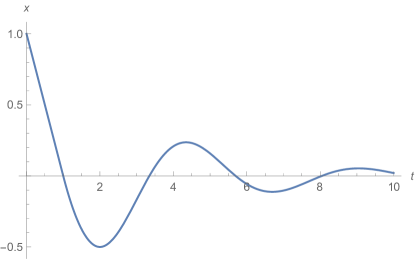
Figure 6.2: The graph of a solution of equation $x^{\prime}(t)=-x(t-1)$ with initial function $\phi\equiv 1$

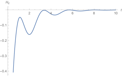
Figure 6.3: The graph of the conditional entropy as given by (6.27) for the example in Figure 6.2 and $\sigma=1/4$

Thus the existence of the delay in the dynamics has modified the temporal trajectory of the conditional entropy from being a monotone increase to equilibrium (in the zero delay case) to one in which the temporal behaviour may well be non-monotone in the approach to equilibrium and can be strongly dependent on the nature of the initial function $\phi(s)$ for $s\in[-\tau,0]$.

Lack of monotonicity of the entropies in one dimensional linear delay dynamics with and without noise

We now show that both the Gibbs’ entropy $H_{G}(f(\cdot,t))$ and the conditional entropy $H_{c}(f(\cdot,t)|f_{*})$ may not be monotone functions of time. To see this we take as the initial distribution a Gaussian distribution. Suppose as in Mackey and Tyran-Kamińska (2021) that the initial condition $x_{0}=\phi$ is a Gaussian process $\xi$ with covariance function $R_{0}$ of the form

$$R_{0}(s_{1},s_{2})=\int_{-\tau}^{0}\eta_{r}(s_{1})\eta_{r}(s_{2})dr,$$ (6.30)

for some function $\eta_{r}\colon[-\tau,0]\to\mathbb{R}$ such that $(s,r)\mapsto\eta_{r}(s)$ is Borel measurable. Then the covariance $R_{t}$ of the Gaussian process $S_{t}\xi$ is given by

$$R_{t}(s_{1},s_{2})=\int_{-\tau}^{0}S_{t}\eta_{r}(s_{1})S_{t}\eta_{r}(s_{2})dr$$

and in particular, for the variance $\sigma^{2}(t)=R_{t}(0,0)$ of $S_{t}\xi(0)$ we have

$$\sigma^{2}(t)=\int_{-\tau}^{0}(S_{t}\eta_{r}(0))^{2}dr.$$

One example of (6.30) is $R_{0}(s_{1},s_{2})=\bar{\sigma}^{2}(\min\{s_{1},s_{2}\}+\tau)$ for $s_{1},s_{2}\in[-\tau,0]$, where $\bar{\sigma}>0$, since (6.30) holds with

$$\eta_{r}(s)=\bar{\sigma}1_{[r,0]}(s),\quad s,r\in[-\tau,0].$$

Then we have $\xi(s)=\bar{\sigma}W(s+\tau)$, where $W=\{W(t)\}_{t\geq 0}$ is a standard Wiener process on $[0,\infty)$. Consider now Eq. 6.14 with $a=0$

$$dx(t)=bx(t-\tau)dt+\sigma dw(t),\quad t>0,$$ (6.31)

and the initial condition

$$x(t)=\xi(t),\quad t\in[-\tau,0],$$

where we assume that $\xi$ is independent of the Wiener process $w$. Then

$$x(t)=S_{t}\xi(0)+y(t)$$

has a Gaussian distribution with mean $0$ and variance $\bar{\sigma}^{2}_{t}$ being the sum of variances of $S_{t}\xi(0)$ and $y(t)$

$$\bar{\sigma}^{2}_{t}=\int_{-\tau}^{0}(S_{t}\eta_{r}(0))^{2}dr+\upsilon(t).$$

It is easily seen that

$$S_{t}\eta_{r}(0)=\bar{\sigma}X(t-r),\quad t\geq 0,r\in[-\tau,0].$$

Thus we obtain

$$\sigma^{2}(t)=\bar{\sigma}^{2}\int_{t}^{t+\tau}X^{2}(q)dq,$$ (6.32)

leading to

$$\bar{\sigma}^{2}_{t}=\frac{\bar{\sigma}^{2}}{\sigma^{2}}\upsilon(t+\tau)+\left(1-\frac{\bar{\sigma}^{2}}{\sigma^{2}}\right)\upsilon(t).$$

Note that if $\bar{\sigma}^{2}>\sigma^{2}$ then $\bar{\sigma}^{2}_{t}$ need not to be a monotone function of time, implying that the Gibbs’s entropy and the conditional entropy of the density $f(x,t)$ of the solution of (6.31) will not be monotone functions of time, see Figures 6.4 and 6.5.

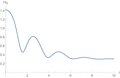
Figure 6.4: The graph of the Gibbs’ entropy for the Gaussian density of the solution of (6.31) with $b=-1$, $\tau=\bar{\sigma}=1$ and $\sigma=1/4$

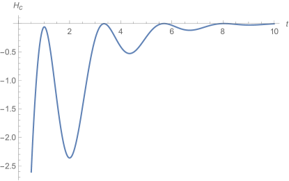
Figure 6.5: The graph of the conditional entropy for the Gaussian density of the solution of (6.31) with $b=-1$, $\tau=\bar{\sigma}=1$ and $\sigma=1/4$

Finally, let us recall that Eq. (6.31) has a stationary solution if and only if

$$-\frac{\pi}{2}<b\tau<0.$$ (6.33)

In that case we have $f(x,t)\to f_{*}(x)$ as $t\to\infty$ by (6.10) and the fact that $p(x,t|\phi)\to f_{*}(x)$ as $t\to\infty$ for each $\phi\in C$ and arbitrary initial distribution.

Now, suppose that $\sigma=0$ in (6.31) and that we start with an initial distribution being Gaussian as above. If condition (6.33) holds then the variance $\sigma^{2}(t)$ of $x(t)$ as given by Eq. 6.32 converges to $0$ as $t\to\infty$ and $0$ is a stationary solution of (6.31), see Mackey and Tyran-Kamińska (2021). If $b=-1$ and $\tau=\pi/2$, then $x(t)$ has a Gaussian density $f(x,t)$ with variance $\sigma^{2}(t)$. The graph of its Gibbs’ entropy is presented in Figure 6.6. It is known Mackey and Tyran-Kamińska (2021) that equation $x^{\prime}(t)=-x(t-\tau)$ with $\tau=\pi/2$ has a non-zero stationary solution in which case $f_{*}(x)$ is the Gaussian density with mean 0 and variance 1. Then the conditional entropy $H_{c}(f(\cdot,t)|f_{*})$ is of the form

$$H_{c}(f(\cdot,t)|f_{*})=\frac{1}{2}\ln\sigma^{2}(t)+\frac{1}{2}(1-\sigma^{2}(t))$$

and its graph is presented in Figure 6.7.

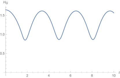
Figure 6.6: The graph of the Gibbs’ entropy for the Gaussian density of the solution of $x^{\prime}(t)=-x(t-\tau)$ with $\tau=\pi/2$, $\bar{\sigma}=1$

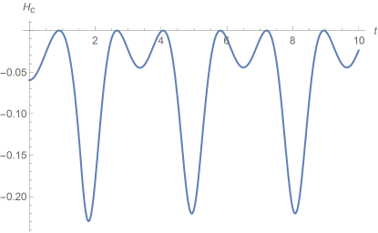
Figure 6.7: The graph of the conditional entropy for the Gaussian density of the solution of $x^{\prime}(t)=-x(t-\tau)$ with $\tau=\pi/2$, $\bar{\sigma}=1$

7 Discussion

It is the universal experience that in all living things there is an inexorable one-way progression of events from birth through aging culminating in death. We never witness the reverse sequence. The rather astonishing thing, however, is that all of the laws (evolution equations) that are written down in physics show no preference for a direction of time. They are all equally valid for time $t$ going in a positive direction as well as in a negative direction, and this is true for the equations of mechanics, electricity and magnetism, special and general relativity and quantum mechanics (Sachs, 1987). Why is there no clear preference for a direction of time in the dynamical equations of physics?

Countless scientists have thought about, and written about, this apparently contradictory situation. In a non-technical vein, Brillouin (1950) has written an extremely thoughtful essay examining a variety of issues related to this question that is informative, deep, and provocative. In his usual fashion, Martin Gardner (1967) has an amusing survey of the problems that would be encountered if time could go backward that is well worth reading and pondering. Finally, Gold (1962) expounds very eloquently on the possibility that temporal irreversibility is cosmologically derived from the (observed) expansion of the universe. This is elaborated on in the essay by Schulman (2010).

Many authors have considered the possible origins of the unidirectionality of time over the years, and without being exhaustive we mention Reichenbach (1957), Fer (1977), Davies (1977), Sachs (1987), Zeh (1992) and Sklar (1993) as those worth reading. There is, in addition, a very useful collection of reprinted musings on the subject in Landsberg (1985), as well as innumerable conference proceedings including Gold and Schumacher (1969), Halliwell et al. (1996), Schulman (1997), and Savitt (1998).

Not surprisingly, since many of those who have considered the possible origins of temporal unidirectionality have been physicists, the issue of the Second Law of Thermodynamics has repeatedly been invoked, examined, and discussed. In the early part of the 20^th century Eddington (1934) re-framed the issue of temporal unidirectionality in terms of the behaviour of entropy, saying:

“The law that entropy always increases holds, I think, the supreme position among the laws of Nature. If someone points out to you that your pet theory of the universe is in disagreement with Maxwell’s equations - then so much the worse for Maxwell’s equations. If it is found to be contradicted by observation - well, these experimentalists do bungle things sometimes. But if your theory is found to be against the Second Law of Thermodynamics I can give you no hope; there is nothing for it to collapse in deepest humiliation.”

Here we have explored only a few of the possibilities for the uni-directionality of time related to the temporal behaviour of entropy. Our considerations are not new except for the results of Section 6, but serve to highlight the nature of the problem. In Table 7.1 we have summarized our results here in terms of the temporal behaviours of $H_{G}$, $H_{c}$, and $H_{NE}$.

Type of dynamics	$H_{c}(f|f_{*})$	$H_{G}(f)$	$H_{NE}(f|f_{*})=H_{c}(f|f_{*})+H_{G}(f_{*})$
Invertible, Sec. 3	$\dot{H}_{c}\equiv 0$, Thm. 3.1, Eq. 3.3	$\dot{H}_{G}(f)\equiv 0$	$\dot{H}_{NE}(f|f_{*})\equiv 0$
Asymptotically stable, Sec. 4	$\lim_{t\to\infty}H_{c}(f|f_{*})=0$, Thm. 4.1	$\lim_{t\to\infty}H_{G}(f)=H_{G}(f_{*})$, Thm. 4.3	$\lim_{t\to\infty}H_{NE}(f|f_{*})=H_{G}(f_{*})$
Stochastic ODE, Sec. 5	$\dot{H}_{c}\geq 0$, Eq. 5.8	$\dot{H}_{G}\,\,\pm$, Eq. 5.15	$\dot{H}_{NE}\geq 0$
Delayed dynamics, Sec. 6	$\dot{H}_{c}\pm$, Fig. 6.7	$\dot{H}_{G}\pm$. Fig. 6.6	$\dot{H}_{NE}\pm$
Delayed stochastic, Sec. 6	$\dot{H}_{c}\pm$, Figs. 6.2, 6.5	$\dot{H}_{G}\pm$. Fig. 6.4	$\dot{H}_{NE}\pm$

Table 7.1: Summary of the behaviours of $H_{c}(P^{t}f|f_{*})$ and $H_{G}(P^{t}f)$ in which we indicate the sign of $\dot{H}_{c}$, $\dot{H}_{G}$, and $\dot{H}_{NE}$.

The non-equilibrium Gibbs’ entropy $H_{G}(f)$ is manifestly not a good candidate for $S_{TD}(t)$ because its dynamical behavior is at odds with what is demanded by the Second Law of Thermodynamics. As we have demonstrated in Mackey and Tyran-Kamińska (2006b) and here, concrete analytic examples can be constructed in which the direction of the temporal change in $H_{G}(f)$ depends on the initial preparation of the system and others can be constructed in which $H_{G}(f)$ oscillates in time.

A number of other authors, including de Groot and Mazur (1984, pp. 122-129, Eq. 247), Van Kampen (1992, pp. 111-114 and 185), and Penrose (2005, p. 213) have suggested that a time dependent entropy should be associated dynamically with

$$H_{NE}(f) \equiv H_{c}(f|f_{*}e^{H_{G}(f_{*})})$$ (7.1)

$$= H_{c}(f|f_{*})+H_{G}(f_{*})$$

as an extension of the Gibbs (1962, pp. 44-45 and 168) discussion of entropy. This also goes under the name of the “Gibbs’ entropy postulate” (P’erez-Madrid et al., 1994; Rub’i and Mazur, 1998; Mazur, 1998; Rub’i and Mazur, 2000; Bedeaux and Mazur, 2001; Rub’i and P’erez-Madrid, 2001).

In the absence of both stochastic perturbation and delays, we have shown that the conditional entropy (and thus $H_{NE}$) is temporally constant. The introduction of stochasticity can induce the monotone approach of $H_{NE}$ to a maximum of zero.

In our quest to extend the problem of entropy evolution to situations with delays, in Section 6 we have considered ‘density’ evolution in stochastically perturbed systems with delayed dynamics like (6.4). We have derived a ‘Fokker-Planck’ like equation (6.7) for the ‘density’. This is exactly analogous to our procedure in Mackey and Tyran-Kamińska (2021) when we derived a ‘Liouville-like’ equation (Mackey and Tyran-Kamińska, 2021, Eqn. 22) for the density evolution under the action of completely deterministic delayed dynamics (Mackey and Tyran-Kamińska, 2021, Eqn. 15). Both of these results for the Liouville and Fokker-Planck like evolution equations are equivalent to those derived by others, e.g. Guillouzic et al. (1999), Loos (2021) although our method of derivation deviates from theirs.

The interesting finding is that the presence of delay can destroy this monotonicity and lead to an oscillatory behaviour of the Gibbs’ and conditional entropy, and thus $H_{NE}$. If stochastic perturbations are simultaneously present then there may be an oscillatory approach of the entropies to a maximum. Thus it would seem that $H_{c}$ and $H_{NE}$ are not viable candidates for a time dependent non-equilibrium entropy if delays play a significant role in entropic behavior in the real world.

The next obvious extension will be to look at nonlinear delayed and stochastic delayed systems though it is not obvious to us how to proceed with this programme.

References

- Abbondandolo (1999) A. Abbondandolo. An H-theorem for a class of Markov processes. Stoch. Anal. Applic., 17:131–136, 1999.
- Arnold et al. (2001) A. Arnold, P. Markowich, G. Toscani, and A. Unterreiter. On convex Sobolev inequalities and the rate of convergence to equilibrium for Fokker-Planck type equations. Comm. Partial Differential Equations, 26:43–100, 2001.
- Bag (2002a) B.C. Bag. Nonequilibrium stochastic processes: time dependence of entropy flux and entropy production. Phys. Rev. E, 66:026122–1–8, 2002a.
- Bag (2002b) B.C. Bag. Upper bound for the time derivative of entropy for nonequilibrium stochastic processes. Phys. Rev. E, 65:046118–1–6, 2002b.
- Bag (2003) B.C. Bag. Information entropy production in non-Markovian systems. J. Chem. Phys., 119:4988–4990, 2003.
- Bakry and Émery (1985) D. Bakry and M. Émery. Diffusions hypercontractives. In Séminaire de probabilités, XIX, 1983/84, volume 1123 of Lecture Notes in Math., pages 177–206. Springer, Berlin, 1985.
- Bedeaux and Mazur (2001) D. Bedeaux and P. Mazur. Mesoscopic non-equilibrium thermodynamics for quantum systems. Physica A, 298:81–100, 2001.
- Brillouin (1950) L. Brillouin. Thermodynamics and information theory. American Scientist, 38(4):594–599, 1950.
- Daems and Nicolis (1999) D. Daems and G. Nicolis. Entropy production and phase space volume contraction. Phys. Rev. E., 59:4000–4006, 1999.
- Davies (1977) P.C.W. Davies. The Physics of Time Asymmetry. Univ of California Press, 1977.
- de Groot and Mazur (1984) S.R. de Groot and P. Mazur. Non-Equilibrium Thermodynamics. Dover, New York, 1984.
- Dynkin (1965) E. B. Dynkin. Markov processes. Vols. I, II. Academic Press Inc., Publishers, New York; Springer-Verlag, Berlin-Göttingen-Heidelberg, 1965.
- Eddington (1934) A. Eddington. New Pathways in Science: Messenger Lectures (1934). Cambridge University Press, 1934.
- Eu (1997) B. C. Eu. Fluctuations and relative Boltzmann entropy. J. Chem. Phys., 106:2388–2399, 1997.
- Fer (1977) F. Fer. L’irréversibilité, Fondement de la Stabilité du Monde Physique. Gauthier-Villars Paris, 1977.
- Gardiner (1983) C.W. Gardiner. Handbook of Stochastic Methods. Springer Verlag, Berlin, Heidelberg, 1983. ISBN 0-387-15607-0.
- Gardner (1967) M. Gardner. Can time go backward? Scientific American, 216(1):98–109, 1967.
- Gibbs (1962) J.W. Gibbs. Elementary Principles in Statistical Mechanics. Dover, New York, 1962.
- Gold (1962) T. Gold. The arrow of time. American Journal of Physics, 30(6):403–410, 1962.
- Gold and Schumacher (1969) T. Gold and D.L. Schumacher. The nature of time. British Journal for the Philosophy of Science, 20(1), 1969.
- Guillouzic et al. (1999) S. Guillouzic, I. L’Heureux, and A. Longtin. Small delay approximation of stochastic delay differential equations. Phys. Rev. E, 61:3970–3982, 1999.
- Hale and Lunel (1993) J.K. Hale and S.M. Verduyn Lunel. Introduction to Functional Differential Equations, volume 99 of Applied Mathematical Sciences. Springer-Verlag, New York, 1993.
- Halliwell et al. (1996) J.J Halliwell, J. Pérez-Mercader, and W.H. Zurek. Physical Origins of Time Asymmetry. Cambridge University Press, 1996.
- Hayes (1950) N.D. Hayes. Roots of the transcendental equation associated with a certain difference-differential equation. J. London Math. Soc. (2), 1(3):226–232, 1950.
- Hill (2013) T.L Hill. Statistical Mechanics: Principles and Selected Applications. Courier Corporation, 2013.
- Horsthemke and Lefever (1984) W. Horsthemke and R. Lefever. Noise Induced Transitions: Theory and Applications in Physics, Chemistry, and Biology. Springer-Verlag, Berlin, New York, Heidelberg, 1984.
- Huang et al. (2019) Xing Huang, Michael Röckner, and Feng-Yu Wang. Nonlinear Fokker-Planck equations for probability measures on path space and path-distribution dependent SDEs. Discrete Contin. Dyn. Syst., 39(6):3017–3035, 2019.
- Kittel (2004) C. Kittel. Elementary Statistical Physics. Courier Corporation, 2004.
- Küchler and Mensch (1992) U. Küchler and B. Mensch. Langevin’s stochastic differential equation extended by a time-delayed term. Stochastics Stochastics Rep., 40(1-2):23–42, 1992.
- Landsberg (1985) P.T. Landsberg. The Enigma of Time. Hilger, 1985.
- Lasota and Mackey (1994) A. Lasota and M. C. Mackey. Chaos, Fractals and Noise: Stochastic Aspects of Dynamics. Springer-Verlag, Berlin, New York, Heidelberg, 1994.
- Loos (2021) S.A.M. Loos. Stochastic Systems with Time Delay: Probabilistic and Thermodynamic Descriptions of Non-Markovian Processes Far from Equilibrium. Springer Nature, 2021.
- Loskot and Rudnicki (1991) K. Loskot and R. Rudnicki. Relative entropy and stability of stochastic semigroups. Ann. Pol. Math., 52:140–145, 1991.
- Losson et al. (2020) J. Losson, M. C. Mackey, R. Taylor, and M. Tyran-Kamińska. Density Evolution Under Delayed Dynamics: An Open Problem, volume 38 of Fields Institute Monographs. Springer, New York, 2020.
- Mackey (2011) M.C Mackey. Time’s Arrow: The Origins of Thermodynamic Behavior. Springer Verlag, 2011.
- Mackey and Nechaeva (1995) M.C. Mackey and I.G. Nechaeva. Solution moment stability in stochastic differential delay equations. Physical Review E, 52(4):3366, 1995.
- Mackey and Tyran-Kamińska (2006a) M.C Mackey and M. Tyran-Kamińska. Noise and conditional entropy evolution. Physica A: Statistical Mechanics and its Applications, 365(2):360–382, 2006a.
- Mackey and Tyran-Kamińska (2006b) M.C. Mackey and M. Tyran-Kamińska. Temporal behavior of the conditional and gibbs’ entropies. Journal of statistical physics, 124:1443–1470, 2006b.
- Mackey and Tyran-Kamińska (2021) M.C. Mackey and M. Tyran-Kamińska. How can we describe density evolution under delayed dynamics? Chaos: An Interdisciplinary Journal of Nonlinear Science, 31(4):043114, 2021.
- Mayer and Mayer (1940) J.E. Mayer and M.G. Mayer. Statistical Mechanics, volume 28. John Wiley & Sons New York, 1940.
- Mazur (1998) P. Mazur. Fluctuations and non-equilibrium thermodynamics. Physica A, 261:451–457, 1998.
- Mohammed (1984) S-E A. Mohammed. Stochastic Functional Differential Equations. Pitman, Boston, 1984.
- Nicolis and Daems (1998) G. Nicolis and D. Daems. Probabilistic and thermodynamic aspects of dynamical systems. Chaos, 8:311–320, 1998.
- Penrose (2005) O. Penrose. Foundations of Statistical Mechanics. Dover, Mineola, New York, revised edition, 2005.
- P’erez-Madrid et al. (1994) A. P’erez-Madrid, J.M. Rub’i, and P. Mazur. Brownian motion in the presence of a temperature gradient. Physica A, 212:231–238, 1994.