Short-flow-time expansion of quark bilinears through next-to-next-to-leading order QCD

Abstract

The gradient-flow formalism proves to be a useful tool in lattice calculations of quantum chromodynamics. For example, it can be used as a scheme to renormalize composite operators by inverting the short-flow-time expansion of the corresponding flowed operators. In this paper, we consider the short-flow-time expansion of five quark bilinear operators, the scalar, pseudoscalar, vector, axialvector, and tensor currents, and compute the matching coefficients through next-to-next-to-leading order quantum chromodynamics (QCD). Among other applications, our results constitute one ingredient for calculating bag parameters of mesons within the gradient-flow formalism on the lattice.

1 Introduction

The gradient-flow formalism (GFF) [1, 2, 3] extends the fields of QCD in terms of the flow time $t$ and is meanwhile an established tool in lattice gauge theory calculations. Its main application up to now has been in the scale setting procedure, required to determine the lattice spacing in physical units [3, 4], as a scheme for defining the strong coupling constant [3, 5, 6, 7, 8, 9, 10], or simply as a smearing mechanism [1, 3]. However, it has been shown that the GFF has a much larger potential. One of the key elements for this is the short-flow-time expansion (SFTX), where composite operators of flowed fields are expressed in terms of a regular operator product expansion (OPE). By inversion of a complete basis of operators, this lets one express an effective Lagrangian in regular QCD in terms of flowed operators and corresponding flowed Wilson coefficients [11, 12, 13, 14]. Matrix elements of the former do not require renormalization [11, 15, 16] and are thus ideally suited to be computed on the lattice. The flowed Wilson coefficients, on the other hand, can be obtained from the regular $\overline{\mathrm{{MS}}}$ results via suitable conversion factors, which can be calculated perturbatively. Obviously, the perturbative order of these conversion factors has to match the one of the regular $\overline{\mathrm{{MS}}}$ Wilson coefficients. This is why, in many cases, next-to-leading order (NLO) results are not sufficient, but higher orders are required.

The feasibility of the above approach was demonstrated via a flowed formulation of the energy-momentum tensor in QCD [12, 13, 17] which was subsequently used to extract thermodynamical observables from the lattice [18, 19, 20, 21, 22, 23, 24, 25, 26, 27]. In this case, the coefficients of the regular operators are rational numbers. It was shown that the next-to-next-to-leading order (NNLO) corrections to the matching matrix, which determines the conversion to flowed operators, lead to a significant improvement in the extrapolation to the physical limit at $t=0$ [23].

As is well known from regular perturbation theory, every additional order leads to an enormous increase in complexity. Fortunately, however, many of the tools and techniques from regular perturbation theory can be adapted to higher orders in the GFF. An outline of this strategy has been described in Ref. [28], where a number of three-loop quantities were evaluated at finite flow time. Using this approach allowed to extend the NLO results for the effective weak $|\Delta F|=2$ Hamiltonian [29] or the magnetic dipole moment operator [30] to the NNLO in Ref. [31] and Ref. [32], respectively. Similarly, the matching matrix between flowed and regular operators and Wilson coefficients was obtained to the same order for the hadronic vacuum polarization [33].

One of the main benefits of the GFF is the exponential suppression of high-momentum modes. As already mentioned above, this implies that composite operators of flowed fields do not require renormalization. Matrix elements of operators which only involve flowed gluons are even finite after renormalization of the regular QCD parameters (strong coupling and masses). Flowed quark fields, on the other hand, still require multiplicative renormalization, typically denoted by $Z_{\chi}$, see Section 2.1. In order to match perturbative and lattice results, one needs to define a suitable renormalization scheme, most conveniently via a Green’s function which involves two flowed quark fields. One option is the so-called ringed scheme, originally proposed in Ref. [13], which fixes $Z_{\chi}$ via the tree-level vacuum expectation value of the quark kinetic operator. The conversion factor between the $\overline{\mathrm{{MS}}}$ and the ringed scheme is known through NNLO [28].

However, other options for the scheme of $Z_{\chi}$ may be more convenient. For example, one may fix it via the SFTX of some quark bilinear operator, usually called current. A preliminary lattice study of this strategy was recently presented in Ref. [34], where the flowed four-quark operator was normalized to the flowed axialvector current. Which current is most suitable may depend on the specific calculation or observable under consideration. It will therefore be useful to have all the associated results at disposal.

Moreover, the simplicity of the quark currents could also be used for systematic studies of the SFTX. First, one can compare perturbative and nonperturbative determinations of the matching coefficients with each other. Some preliminary studies in this direction have already been carried out in Ref. [35] for the CP-violating quark chromoelectric dipole moment operator and for the currents in Ref. [36]. Secondly, one can compare results for the renormalized currents obtained through the SFTX with results obtained in more conventional non-perturbative schemes. This may allow one to test non-perturbatively the accuracy of the SFTX and assess the systematics associated with the $t\to 0$ limit. A first study of higher-power terms has been done in the context of the energy-momentum tensor in Ref. [26]. Besides these indirect applications, the SFTX of the currents directly contribute to a number of observables in the GFF such as the chiral condensate [19] or semileptonic contributions to the neutron electric dipole moment [37].

Through NLO, the SFTX of the currents has been calculated already several years ago [38, 39]. In order to be consistent with the uncertainties expected from the associated lattice calculations, one can expect that higher orders of the matching coefficients will be relevant. In this paper, we will therefore derive the corresponding NNLO results.

The remainder of this paper is structured as follows: In Section 2, we discuss the theoretical basis of our calculation, starting with the GFF in Section 2.1, the definition of the regular and flowed currents in Section 2.2, and the methods to obtain the SFTX in Section 2.3. Our results for the matching coefficients are presented in Section 3. The latter also allow us to evaluate the so-called flowed anomalous dimensions, describing the logarithmic flow-time evolution of the currents. This is presented in Section 4. Section 5 contains our conclusions.

2 Theoretical framework

2.1 The QCD gradient flow

In this paper, we work in $D$-dimensional Euclidean space-time with $D=4-2\epsilon$. The GFF continues the gluon and quark fields $A_{\mu}$ and $\psi$ of regular QCD to fields $B_{\mu}(t)$ and $\chi(t)$ through the initial conditions

$$\begin{split}B_{\mu}(t=0)=A_{\mu}\,,\qquad\chi(t=0)=\psi\,,\end{split}$$ (2.1)

and the flow equations [1, 3, 15]

$$\begin{split}\partial_{t}B_{\mu}&=\mathcal{D}_{\nu}G_{\nu\mu}+\kappa\mathcal{D}_{\mu}\partial_{\nu}B_{\nu}\,,\\ \partial_{t}\chi&=\Delta\chi-\kappa\,g_{\text{{B}}}\partial_{\mu}B_{\mu}\chi\,,\\ \partial_{t}\bar{\chi}&=\bar{\chi}\overleftarrow{\Delta}+\kappa\,g_{\text{{B}}}\bar{\chi}\partial_{\mu}B_{\mu}\,,\end{split}$$ (2.2)

where the “flow time” $t$ is a parameter of mass dimension $[t]=-2$, $g_{\text{{B}}}$ is the bare strong coupling, and $\kappa$ is a gauge parameter which drops out of physical observables. In our calculations, we set $\kappa=1$.

The flowed field-strength tensor is defined as

$$G_{\mu\nu}=\partial_{\mu}B_{\nu}-\partial_{\nu}B_{\mu}+g_{\text{{B}}}[B_{\mu},B_{\nu}]\,,$$ (2.3)

the flowed covariant derivative in the adjoint representation is given by

$$\mathcal{D}_{\mu}=\partial_{\mu}+g_{\text{{B}}}[B_{\mu},\cdot\,]\,,$$ (2.4)

and

$$\begin{split}\Delta=\mathcal{D}^{\mathrm{F}}_{\mu}\mathcal{D}^{\mathrm{F}}_{\mu}\,,\qquad\overleftarrow{\Delta}=\overleftarrow{\mathcal{D}}^{\mathrm{F}}_{\mu}\overleftarrow{\mathcal{D}}^{\mathrm{F}}_{\mu}\,,\end{split}$$ (2.5)

with the flowed covariant derivative in the fundamental representation,

$$\mathcal{D}^{\mathrm{F}}_{\mu}=\partial_{\mu}+g_{\text{{B}}}B_{\mu}\,,\qquad\overleftarrow{\mathcal{D}}^{\mathrm{F}}_{\mu}=\overleftarrow{\partial}_{\mu}-g_{\text{{B}}}B_{\mu}\,.$$ (2.6)

The flow equations can be solved perturbatively, leading to generalized QCD Feynman rules which involve exponential factors for the quark and gluon propagators, plus additional “flow-lines” representing the evolution of the fields in the flow time. The latter couple to the quarks and gluons via “flowed vertices”. The general formalism has been worked out in Refs. [11, 15], and more details can be found in Ref. [28].

Since the flow time acts as regulator for ultraviolet divergences, the GFF improves the renormalization properties. After renormalization of the fundamental parameters of QCD, the flowed gluon field $B_{\mu}(t)$ is finite and does not require field renormalization [3, 11, 16]. The flowed quark fields $\chi(t)$, on the other hand, require multiplicative field renormalization [15]. Throughout this paper, we will adopt the ringed scheme [13], where

$$\mathring{\chi}=\mathring{Z}_{\chi}^{1/2}\chi\,,\qquad\mathring{Z}_{\chi}=\zeta_{\chi}\,Z^{\overline{\mathrm{{MS}}}}_{\chi}\,.$$ (2.7)

Both the $\overline{\mathrm{{MS}}}$ expression $Z^{\overline{\mathrm{{MS}}}}_{\chi}$ as well as the finite conversion factor to the ringed scheme, $\zeta_{\chi}$, are available through NNLO [15, 13, 17, 28]. Explicit expressions are collected in Appendix A.

Parameter and field renormalization are sufficient to render physical matrix elements of composite operators finite [11, 15, 16]. Thus, composite flowed operators do not mix under renormalization, which enormously facilitates the lattice evaluation of their matrix elements compared to those of regular operators, in particular if the latter mix with operators of different mass dimension. Connection of the flowed matrix elements to physics at $t=0$ can be made through a perturbative calculation, as will be explained in more detail in Section 2.3.

2.2 Quark currents

In this paper, we consider $n_{\text{f}}=n_{\text{l}}+n_{\text{h}}$ quark flavors, where $n_{\text{l}}$ is the number of massless quarks, while the remaining $n_{\text{h}}$ quarks have identical mass $m$. The bare non-diagonal and diagonal currents are defined as

$$j_{pq}^{\text{{B}}} =\bar{\psi}_{p}\Gamma\psi_{q}\,, j_{p}^{\text{{B}}} =\bar{\psi}_{p}\Gamma\psi_{p}\,,$$ (2.8)

respectively, where $p$ and $q$ are flavor indices with $p\neq q$. We furthermore define the bare and renormalized singlet and non-singlet currents as

$$j^{a,\text{ns}}_{\text{{B}}} =\sum_{p\neq q}h^{a}_{pq}\,j^{\text{{B}}}_{pq}+\sum_{p}h^{a}_{pp}\,j^{\text{{B}}}_{p}\,, j^{\text{s}}_{\text{{B}}} =\sum_{p}j^{\text{{B}}}_{p}\,,$$ (2.9)

$$j^{a,\text{ns}} =Z^{\text{ns}}j^{a,\text{ns}}_{\text{{B}}}\,, j^{\text{s}} =Z^{\text{s}}j^{\text{s}}_{\text{{B}}}-4Z_{m}^{-3}Z_{\mathds{1}}m_{\text{{B}}}^{3}\mathds{1}\,,$$

where $h^{a}$ is a traceless flavor generator, and $m_{\text{{B}}}$ is the bare quark mass which is related to the $\overline{\mathrm{{MS}}}$ renormalized mass $m$ through

$$m_{\text{{B}}}=Z_{m}\,m\,,$$ (2.10)

with $Z_{m}\equiv Z_{m}^{\overline{\mathrm{{MS}}}}$ given in Eqs. A.6 and A.12. $Z^{\text{s}}$, $Z^{\text{ns}}$, and $Z_{\mathds{1}}$ are renormalization constants which will be specified below. They depend on the Dirac structure $\Gamma\in\{\Gamma_{\text{S}},\Gamma_{\text{V}}^{\mu},\Gamma_{\text{T}}^{\mu\nu},\Gamma_{\text{A}}^{\mu},\Gamma_{\text{P}}\}$ of the current, where

$$\Gamma_{\text{S}} =1\,, \qquad\Gamma_{\text{V}}^{\mu} =\gamma^{\mu}\,, \qquad\Gamma_{\text{T}}^{\mu\nu} =\sigma^{\mu\nu}\equiv\frac{1}{2}\left[\gamma^{\mu},\gamma^{\nu}\right]\,,$$ (2.11)

$$\quad\Gamma_{\text{A}}^{\mu} =\gamma^{\mu}\gamma_{5}\,, \qquad\Gamma_{\text{P}} =\gamma_{5}\,,$$

i.e. we consider the parity-even scalar, vector, and tensor currents, and the parity-odd axialvector and pseudoscalar currents. The renormalization constant $Z_{\mathds{1}}$ allows for the possibility of the currents to mix with the unit operator.

2.3 Short-flow-time expansion

Returning to the non-diagonal and diagonal notation, we define the flowed currents as

$$\tilde{j}_{pq}(t) =\mathring{Z}_{\chi}\,\bar{\chi}_{p}(t)\Gamma\chi_{q}(t)\,, \tilde{j}_{p}(t) =\mathring{Z}_{\chi}\,\bar{\chi}_{p}(t)\Gamma\chi_{p}(t)\,,$$ (2.12)

which means that we adopt the ringed scheme for the flowed quark renormalization throughout this paper, unless stated otherwise. The flowed singlet and non-singlet currents are defined by replacing the diagonal and non-diagonal currents by their flowed versions.

The SFTX [11] for the singlet and non-singlet current can be written as

$$\tilde{j}^{a,\text{ns}}(t) =\zeta_{\text{{B}}}^{\text{ns}}(t)\,j^{a,\text{ns}}_{\text{{B}}}+\mathcal{O}(t)\equiv\zeta^{\text{ns}}(t)\,j^{a,\text{ns}}+\mathcal{O}(t)\,,$$ (2.13)

$$\tilde{j}^{\text{s}}(t) =n_{\text{h}}m_{\text{{B}}}\left[\frac{1}{t}\zeta_{\text{{B}}}^{(1)}(t)+m^{2}_{\text{{B}}}\,\zeta_{\text{{B}}}^{(3)}(t)\right]\mathds{1}+\zeta_{\text{{B}}}^{\text{s}}(t)\,j^{\text{s}}_{\text{{B}}}+\mathcal{O}(t)$$

$$\equiv n_{\text{h}}m\left[\frac{1}{t}\zeta^{(1)}(t)+m^{2}\,\zeta^{(3)}(t)\right]\mathds{1}+\zeta^{\text{s}}(t)\,j^{\text{s}}+\mathcal{O}(t)\,,$$

where we have taken into account that we only have $n_{\text{h}}$ massive quarks of equal mass $m$. The terms of order $t$ will be neglected in this paper.

The dependence of the matching coefficients $\zeta(t)$ on the flow time $t$ is logarithmic. They are most conveniently computed by defining projectors onto the regular-QCD (i.e. not flowed) diagonal and non-diagonal currents. In our case, we choose

$$P^{(1)}[\mathcal{O}] =t\frac{\partial}{\partial m_{\text{{B}}}}\langle 0|\mathcal{O}|0\rangle\bigg{|}_{m_{\text{{B}}}=0}\,,\qquad P^{(3)}[\mathcal{O}]=\frac{1}{3!}\frac{\partial^{3}}{\partial m_{\text{{B}}}^{3}}\langle 0|\mathcal{O}|0\rangle\bigg{|}_{m_{\text{{B}}}=0}\,,$$ (2.14)

and

$$P_{pq}[\mathcal{O}] =\mathcal{N}^{-1}\text{Tr}(\Gamma\mathcal{M}_{pq}(q_{1},q_{2}))\bigg{|}_{q_{1}=q_{2}=m=0}\,,$$ (2.15)

where $\mathcal{M}_{pq}$ is a two-quark Green’s function defined as

$$\int\mathrm{d}^{4}x\langle\psi_{p}(q_{1})|\mathcal{O}|\psi_{q}(q_{2})\rangle =\bar{u}_{p}(q_{1})\mathcal{M}_{pq}(q_{1},q_{2})u_{q}(q_{2})\,,$$ (2.16)

the trace is over spinor and color indices, and

$$\mathcal{N}=\text{Tr}\left(\Gamma\Gamma\right)\,.$$ (2.17)

The nullification of the masses and external momenta in Eqs. 2.14 and 2.15 is understood to be taken before any loop integral is evaluated. This means that only tree-level diagrams contribute when the projectors are applied to the r.h.s. of Eq. 2.13, because all higher-order diagrams are scaleless and thus vanish in dimensional regularization.

The matching coefficients are then obtained as

$$\zeta^{\text{ns}}_{\text{{B}}}=P_{pq}[\tilde{j}_{pq}]\qquad\text{and}\qquad\zeta^{\text{s}}_{\text{{B}}}=\zeta^{\text{ns}}_{\text{{B}}}+n_{\text{f}}\zeta^{\Delta}_{\text{{B}}}\,,$$ (2.18)

where

$$\zeta^{\Delta}_{\text{{B}}}=P_{pp}[\tilde{j}_{q}]\,,$$ (2.19)

with $p\neq q$, and

$$\zeta^{(1)}_{\text{{B}}}(t) =P^{(1)}[\tilde{j}_{p}]\,, \zeta^{(3)}_{\text{{B}}}(t) =P^{(3)}[\tilde{j}_{p}]\,,$$ (2.20)

for a massive quark flavor $p$. The renormalized matching coefficients follow from this by inserting Eq. 2.9 into Eq. 2.13:

$$\zeta^{(1)}(t) =Z_{m}\,\zeta^{(1)}_{\text{{B}}}(t)\,,$$ (2.21)

$$\zeta^{(3)}(t) =Z^{3}_{m}\zeta^{(3)}_{\text{{B}}}(t)+\frac{4}{n_{\text{h}}}Z_{\mathds{1}}(Z^{\text{s}})^{-1}\zeta^{\text{s}}_{\text{{B}}}\,,$$

$$\zeta^{\text{ns}}(t) =(Z^{\text{ns}})^{-1}\zeta_{\text{{B}}}^{\text{ns}}(t)\,,$$

$$\zeta^{\text{s}}(t) =(Z^{\text{s}})^{-1}\left[\zeta_{\text{{B}}}^{\text{ns}}(t)+n_{\text{f}}\zeta_{\text{{B}}}^{\Delta}(t)\right]=(Z^{\text{s}})^{-1}Z^{\text{ns}}\zeta^{\text{ns}}(t)+n_{\text{f}}(Z^{\text{s}})^{-1}\zeta_{\text{{B}}}^{\Delta}(t)$$

$$\equiv\zeta^{\text{ns}}(t)+n_{\text{f}}\zeta^{\Delta}(t)\,,$$

$$\Rightarrow\ \zeta^{\Delta}(t) =(Z^{\text{s}})^{-1}\left[\zeta_{\text{{B}}}^{\Delta}(t)-\frac{1}{n_{\text{f}}}(Z^{\text{s}}-Z^{\text{ns}})\zeta^{\text{ns}}(t)\right]\,.$$

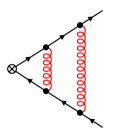
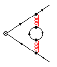
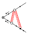
$\zeta_{\text{{B}}}^{(1)}$ and $\zeta_{\text{{B}}}^{(3)}$ are just given by the first two terms in an expansion in $m_{\text{{B}}}^{2}t$ of the currents’ vacuum expectation values. Due to Lorentz and parity invariance, they are non-zero only for the scalar current, corresponding to the so-called quark condensate. Since the one-loop contribution is of order $g_{\text{{B}}}^{0}$, it is required to three-loop order in order to obtain the SFTX up to NNLO QCD. Sample three-loop diagrams are shown in Fig. 1.

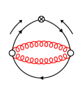(a)	(b)	(c)	(d)

Figure 1: Sample diagrams contributing to $\zeta^{(1)}$ and $\zeta^{(3)}$. Spiral lines are gluons, straight lines denote quarks; lines with accompanying arrows are the corresponding flow lines (they are always connected to flowed vertices, denoted by small circles). The two fermion lines in diagram (c) can be of different flavor. The vertex with the cross denotes the current. All Feynman diagrams in this paper have been drawn with FeynGame [40].

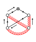
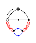
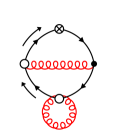
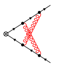
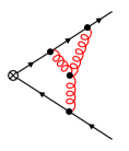
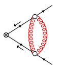
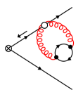
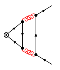
In contrast, the projections for the other matching coefficients in Eq. 2.20 require only two-loop calculations. In the diagrams that contribute to $\zeta^{\text{ns}}_{\text{{B}}}$, the current is connected to the external states by a single quark line, cf. Fig. 2, as opposed to $\zeta_{\text{{B}}}^{\Delta}$, where the current and the external states belong to different quark lines, cf. Fig. 3.

Figure 2: Examples for contributions to the non-singlet matching coefficients. The notation is the same as in Fig. 1.

Figure 3: Examples for contributions to the singlet matching coefficients. The notation is the same as in Fig. 1.

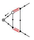We will refer to the latter class as triangle diagrams in what follows. The triangle diagrams for the scalar, pseudoscalar, and tensor currents vanish after taking the fermion trace. For the vector current, they only start to contribute from three-loop order due to Furry’s theorem. At the perturbative order considered here, we can therefore drop the superscripts “ns” and “s” in these cases and simply write

$$\zeta_{\text{X}}(t)\equiv\zeta_{\text{X}}^{\text{ns}}(t)=\zeta^{\text{s}}_{\text{X}}(t)\quad\text{for}\quad\text{X}\neq\text{A}\,,$$ (2.22)

and analogously for the bare matching coefficients. For the axial current, on the other hand, we will find $\zeta_{\text{{B}}}^{\Delta}\neq 0$ at the two-loop level.

We evaluate all diagrams in $D=4-2\epsilon$ space-time dimensions. The occurrence of $\gamma_{5}$ in Eq. 2.11 causes the well-known complications which we take care of by following the strategy outlined in Refs. [41, 42, 43]. This means to replace

$$\Gamma_{\text{A}}^{\mu} \to\hat{\Gamma}_{\text{A}}^{\mu}=\frac{1}{3!}\varepsilon^{\mu\alpha\beta\gamma}\gamma_{\alpha}\gamma_{\beta}\gamma_{\gamma}\,, \Gamma_{\text{P}} \to\hat{\Gamma}_{\text{P}}=\frac{1}{4!}\varepsilon^{\alpha\beta\gamma\delta}\gamma_{\alpha}\gamma_{\beta}\gamma_{\gamma}\gamma_{\delta}$$ (2.23)

both in the currents of Eq. 2.12 as well as in the projectors of Eq. 2.15. The resulting products of two (intrinsically four-dimensional) $\varepsilon$ tensors are replaced by

$$\varepsilon^{\alpha\beta\gamma\delta}\varepsilon_{\alpha^{\prime}\beta^{\prime}\gamma^{\prime}\delta^{\prime}} =g^{[\alpha\phantom{]}}_{\phantom{[}\alpha^{\prime}\phantom{]}}g^{\phantom{[}\beta\phantom{]}}_{\phantom{[}\beta^{\prime}\phantom{]}}g^{\phantom{[}\gamma\phantom{]}}_{\phantom{[}\gamma^{\prime}\phantom{]}}g^{\phantom{[}\delta]}_{\phantom{[}\delta^{\prime}\phantom{]}}\,, \varepsilon^{\mu\alpha\beta\gamma}\varepsilon_{\mu\alpha^{\prime}\beta^{\prime}\gamma^{\prime}} =g^{[\alpha\phantom{]}}_{\phantom{[}\alpha^{\prime}\phantom{]}}g^{\phantom{[}\beta\phantom{]}}_{\phantom{[}\beta^{\prime}\phantom{]}}g^{\phantom{[}\gamma]}_{\phantom{[}\gamma^{\prime}\phantom{]}}\,,$$ (2.24)

where the square brackets denote the anti-symmetric combination, e.g.

$$g^{[\alpha\phantom{]}}_{\phantom{[}\alpha^{\prime}\phantom{]}}g^{\phantom{[}\beta]}_{\phantom{[}\beta^{\prime}\phantom{]}}=g^{\alpha}_{\alpha^{\prime}}g^{\beta}_{\beta^{\prime}}-g^{\beta}_{\alpha^{\prime}}g^{\alpha}_{\beta^{\prime}}\,.$$ (2.25)

This also affects the normalization factors of Eq. 2.17 via

$$\text{Tr}(\hat{\Gamma}_{\text{A}}^{\mu}\hat{\Gamma}_{\text{A}}^{\mu}) =-\frac{2n_{\text{c}}}{3}D(D-1)(D-2)\,,$$ (2.26)

$$\text{Tr}(\hat{\Gamma}_{\text{P}}\hat{\Gamma}_{\text{P}}) =-\frac{n_{\text{c}}}{3!}D(D-1)(D-2)(D-3)\,.$$

This strategy violates the Ward identities, but they can be restored by an additional finite renormalization discussed below.

For the actual calculation, we adopt the framework developed in Ref. [28], which is based on qgraf [44, 45] for the generation of the diagrams, q2e/exp [46, 47] for inserting the Feynman rules and identifying the momentum topologies, in-house FORM [48, 49, 50] routines for performing various computer algebraic operations including Dirac and color algebra [51], and Kira$\otimes$FireFly [52, 53, 54, 55] for the reduction to master integrals employing integration-by-parts-like relations [56, 57, 28] and the Laporta algorithm [58]. Up to two-loop level, we find the same master integrals as in Ref. [17]. They can be evaluated analytically in terms of the transcendentals

$$\zeta_{2}=\text{Li}_{2}(1) =\frac{\pi^{2}}{6}=1.64493\ldots\,,\qquad\zeta_{3}=\text{Li}_{3}(1)=1.20205\ldots\,,$$ (2.27)

$$\text{Li}_{2}(1/4) =0.267652\ldots\,,$$

where $\text{Li}_{n}(z)=\sum_{k=1}^{\infty}z^{k}/k^{n}$ is the polylogarithm of order $n$.

The three-loop vacuum expectation value contributing to $\zeta^{(1)}$ and $\zeta^{(3)}$ of Eq. 2.21 leads to $304$ diagrams which are reduced to 216 master integrals already contributing to Ref. [33]. They have been evaluated numerically following the strategy described in Ref. [59].

3 Results

Parity-even currents.

For the currents which do not involve $\gamma_{5}$, we adopt the $\overline{\mathrm{{MS}}}$ scheme, i.e., we define the renormalization constants of Eq. 2.8 as

$$Z_{\text{X}} =Z_{\text{X}}^{\overline{\mathrm{{MS}}}}\,,\qquad\text{X}\in\{\text{S},\text{V},\text{T}\}\,.$$ (3.1)

Because of Lorentz and parity invariance, only the scalar current can mix with the identity operator. Thus, we have

$$Z_{\mathds{1},\text{S}}=Z_{\mathds{1},\text{S}}^{\overline{\mathrm{{MS}}}} =\left(\frac{\mu^{2}e^{\gamma_{\text{E}}}}{4\pi}\right)^{-\epsilon}Z_{0}\qquad\text{and}\qquad Z_{\mathds{1},\text{X}}=0\,,\qquad\text{X}\in\{\text{V},\text{P},\text{A},\text{T}\}\,,$$ (3.2)

where $Z_{0}$ is the renormalization constant of the vacuum energy which can be found in Eq. A.14, and $\mu$ is the renormalization scale in the $\overline{\mathrm{{MS}}}$ scheme, and $\gamma_{\text{E}}=-\Gamma^{\prime}(1)=0.577216\ldots$ is the Euler-Mascheroni constant, with Euler’s gamma function $\Gamma(z)$. The Ward-Takahashi identities ensure that $Z_{\text{V}}^{\overline{\mathrm{{MS}}}}=1$ and $Z_{\text{S}}^{\overline{\mathrm{{MS}}}}=Z_{m}$, with $Z_{m}$ the quark mass renormalization constant introduced above. For the tensor current, the renormalization constant is given in Eqs. A.5 and A.16.

We express our results in terms of the color factors

$$C_{\text{F}} =T_{\text{R}}\,\frac{n_{\text{c}}^{2}-1}{n_{\text{c}}}\,,\qquad C_{\text{A}}=2T_{\text{R}}n_{\text{c}}\,,\qquad T_{\text{R}}=\frac{1}{2}\,,$$ (3.3)

where in QCD, the number of colors is $n_{\text{c}}=3$. Furthermore, we introduce

$$L_{\mu t}=\ln 2\mu^{2}t+\gamma_{\text{E}}\equiv\ln\frac{\mu^{2}}{\mu_{t}^{2}}\,,$$ (3.4)

where we have implicitly defined the $t$-dependent energy scale $\mu_{t}$, and

$$a_{\text{s}}=\frac{g^{2}}{4\pi^{2}}=\frac{\alpha_{s}}{\pi}\,,$$ (3.5)

with $g$ the $\overline{\mathrm{{MS}}}$ renormalized strong coupling, see Eq. A.1. We then find the following matching coefficients for the parity-even currents:

$$\zeta_{\text{S}}^{(1)}(t) =-\frac{n_{\text{c}}}{8\pi^{2}}\Bigg{\{}1+a_{\text{s}}\,C_{\text{F}}\Big{(}1+\ln 2-\frac{3}{4}\ln 3+\frac{3}{4}L_{\mu t}\Big{)}$$

$$\hskip 10.00002pt+a_{\text{s}}^{2}\bigg{[}1.228\,C_{\text{F}}^{2}+2.587\,C_{\text{A}}C_{\text{F}}-0.9873\,C_{\text{F}}T_{\text{R}}n_{\text{f}}$$

$$\hskip 20.00003pt+L_{\mu t}\big{(}0.7456\,C_{\text{F}}^{2}+1.807\,C_{\text{A}}C_{\text{F}}-0.4981\,C_{\text{F}}T_{\text{R}}n_{\text{f}}\big{)}$$

$$\hskip 20.00003pt+L_{\mu t}^{2}\big{(}0.2813\,C_{\text{F}}^{2}+0.3438\,C_{\text{A}}C_{\text{F}}-0.1250\,C_{\text{F}}T_{\text{R}}n_{\text{f}}\big{)}\bigg{]}\Bigg{\}}+\mathcal{O}(a_{\text{s}}^{3})\,,$$ (3.6)

$$\zeta_{\text{S}}^{(3)}(t) =-\frac{n_{\text{c}}}{4\pi^{2}}\Bigg{\{}1+L_{\mu t}+a_{\text{s}}\,C_{\text{F}}\Bigg{[}\frac{7}{2}+4\ln 2-\frac{21}{4}\ln 3-3\text{Li}_{2}\left(1/4\right)$$

$$\hskip 20.00003pt+L_{\mu t}\bigg{(}\frac{11}{4}-\ln 2-\frac{3}{4}\ln 3\bigg{)}+\frac{3}{4}L_{\mu t}^{2}\Bigg{]}$$

$$\hskip 10.00002pt+a_{\text{s}}^{2}\bigg{(}5.455\,C_{\text{F}}^{2}+0.1028\,C_{\text{A}}C_{\text{F}}-\big{(}1.078\,n_{\text{l}}+6.411\,n_{\text{h}}\big{)}C_{\text{F}}T_{\text{R}}$$

$$\hskip 20.00003pt+L_{\mu t}\big{[}3.095\,C_{\text{F}}^{2}+0.3964\,C_{\text{A}}C_{\text{F}}-\big{(}0.1512\,n_{\text{l}}+3.151\,n_{\text{h}}\big{)}C_{\text{F}}T_{\text{R}}\big{]}$$

$$\hskip 20.00003pt+L_{\mu t}^{2}\big{[}1.862\,C_{\text{F}}^{2}+0.6510\,C_{\text{A}}C_{\text{F}}-0.07763\,C_{\text{F}}T_{\text{R}}n_{\text{f}}\big{]}$$

$$\hskip 20.00003pt+L_{\mu t}^{3}\big{[}0.6563\,C_{\text{F}}^{2}+0.1146\,C_{\text{A}}C_{\text{F}}-0.04167\,C_{\text{F}}T_{\text{R}}n_{\text{f}}\big{]}\bigg{)}\Bigg{\}}+\mathcal{O}(a_{\text{s}}^{3})\,,$$ (3.7)

$$\zeta_{\text{S}}(t) =1+a_{\text{s}}\,C_{\text{F}}\Big{(}-\frac{1}{2}-\ln 2-\frac{3}{4}\ln 3-\frac{3}{4}L_{\mu t}\Big{)}$$

$$\hskip 10.00002pt+a_{\text{s}}^{2}\Bigg{\{}\frac{1}{16}c_{\chi}^{(2)}+C_{\text{F}}^{2}\Big{(}\frac{1}{2}+\frac{1}{2}\zeta_{2}-\frac{3}{2}\ln 2+\frac{1}{4}\ln^{2}2+\frac{21}{8}\ln 3+3\text{Li}_{2}\left(1/4\right)\Big{)}$$

$$\hskip 20.00003pt+C_{\text{A}}C_{\text{F}}\Big{(}-\frac{197}{48}-\frac{7}{16}\zeta_{2}-\frac{9}{2}\ln 2+\frac{1}{4}\ln^{2}2+\frac{9}{2}\ln 3+\frac{3}{2}\text{Li}_{2}\left(1/4\right)\Big{)}$$

$$\hskip 20.00003pt+C_{\text{F}}T_{\text{R}}n_{\text{f}}\Big{(}\frac{5}{6}+\frac{1}{4}\zeta_{2}\Big{)}+L_{\mu t}\bigg{[}C_{\text{F}}^{2}\Big{(}\frac{3}{4}\ln 2+\frac{9}{16}\ln 3+\frac{9}{32}\Big{)}$$

$$\hskip 30.00005pt+C_{\text{A}}C_{\text{F}}\Big{(}-\frac{11}{12}\ln 2-\frac{11}{16}\ln 3-\frac{47}{32}\Big{)}+C_{\text{F}}T_{\text{R}}n_{\text{f}}\Big{(}\frac{1}{3}\ln 2+\frac{1}{4}\ln 3+\frac{3}{8}\Big{)}\bigg{]}$$

$$\hskip 20.00003pt+L_{\mu t}^{2}\bigg{(}\frac{9}{32}C_{\text{F}}^{2}-\frac{11}{32}C_{\text{A}}C_{\text{F}}+\frac{1}{8}C_{\text{F}}T_{\text{R}}n_{\text{f}}\bigg{)}\Bigg{\}}+\mathcal{O}(a_{\text{s}}^{3})\,,$$ (3.8)

$$\zeta_{\text{V}}(t) =1+a_{\text{s}}\,C_{\text{F}}\Big{(}\frac{1}{8}-\ln 2-\frac{3}{4}\ln 3\Big{)}$$

$$\hskip 10.00002pt+a_{\text{s}}^{2}\Bigg{\{}\frac{1}{16}c_{\chi}^{(2)}+C_{\text{F}}^{2}\Big{(}-\frac{41}{128}-\frac{5}{32}\zeta_{2}+\frac{3}{8}\ln 2+\frac{1}{4}\ln^{2}2-\frac{3}{32}\ln 3+\frac{3}{2}\text{Li}_{2}\left(1/4\right)\Big{)}$$

$$\hskip 20.00003pt+C_{\text{A}}C_{\text{F}}\Big{(}-\frac{763}{384}-\frac{5}{32}\zeta_{2}-\frac{13}{4}\ln 2+\frac{1}{4}\ln^{2}2+\frac{27}{8}\ln 3+\frac{21}{16}\text{Li}_{2}\left(1/4\right)\Big{)}$$

$$\hskip 20.00003pt+C_{\text{F}}T_{\text{R}}n_{\text{f}}\Big{(}\frac{35}{96}+\frac{1}{8}\zeta_{2}\Big{)}+L_{\mu t}\bigg{[}C_{\text{A}}C_{\text{F}}\Big{(}-\frac{11}{12}\ln 2-\frac{11}{16}\ln 3+\frac{11}{96}\Big{)}$$

$$\hskip 30.00005pt+C_{\text{F}}T_{\text{R}}n_{\text{f}}\Big{(}\frac{1}{3}\ln 2+\frac{1}{4}\ln 3-\frac{1}{24}\Big{)}\bigg{]}\Bigg{\}}+\mathcal{O}(a_{\text{s}}^{3})\,,$$ (3.9)

$$\zeta_{\text{T}}(t) =1+a_{\text{s}}\,C_{\text{F}}\Big{(}-\ln 2-\frac{3}{4}\ln 3+\frac{1}{4}L_{\mu t}\Big{)}$$

$$\hskip 10.00002pt+a_{\text{s}}^{2}\Bigg{\{}\frac{1}{16}c_{\chi}^{(2)}+C_{\text{F}}^{2}\Big{(}-\frac{7}{12}-\frac{1}{4}\zeta_{2}+\frac{4}{3}\ln 2+\frac{1}{4}\ln^{2}2-\frac{3}{4}\ln 3+\text{Li}_{2}\left(1/4\right)\Big{)}$$

$$\hskip 20.00003pt+C_{\text{A}}C_{\text{F}}\Big{(}-\frac{1159}{864}-\frac{1}{16}\zeta_{2}-\frac{17}{6}\ln 2+\frac{1}{4}\ln^{2}2+3\ln 3+\frac{5}{4}\text{Li}_{2}\left(1/4\right)\Big{)}$$

$$\hskip 20.00003pt+C_{\text{F}}T_{\text{R}}n_{\text{f}}\Big{(}\frac{47}{216}+\frac{1}{12}\zeta_{2}\Big{)}+L_{\mu t}\bigg{[}C_{\text{F}}^{2}\Big{(}-\frac{1}{4}\ln 2-\frac{3}{16}\ln 3-\frac{19}{32}\Big{)}$$

$$\hskip 30.00005pt+C_{\text{A}}C_{\text{F}}\Big{(}-\frac{11}{12}\ln 2-\frac{11}{16}\ln 3+\frac{257}{288}\Big{)}+C_{\text{F}}T_{\text{R}}n_{\text{f}}\Big{(}\frac{1}{3}\ln 2+\frac{1}{4}\ln 3-\frac{13}{72}\Big{)}\bigg{]}$$

$$\hskip 20.00003pt+L_{\mu t}^{2}\bigg{(}\frac{1}{32}C_{\text{F}}^{2}+\frac{11}{96}C_{\text{A}}C_{\text{F}}-\frac{1}{24}C_{\text{F}}T_{\text{R}}n_{\text{f}}\bigg{)}\Bigg{\}}+\mathcal{O}(a_{\text{s}}^{3})\,.$$ (3.10)

$c_{\chi}^{(2)}$ is associated with the ringed scheme and would not appear if the fermions were renormalized in the $\overline{\mathrm{{MS}}}$ scheme. Its explicit form is given in Eqs. A.24 and A.25. The results for $\zeta_{\text{S}}^{(1)}(t)$ and $\zeta_{\text{S}}$ are already known from Refs. [15, 28, 30, 32]. For the sake of brevity, we only quote the three-loop results with four significant digits here. In the ancillary file accompanying this paper, we provide the results with higher numerical accuracy, as well as analytic expressions for the logarithmic terms and the coefficient of $C_{\text{F}}T_{\text{R}}n_{\text{f}}$ of $\zeta_{\text{S}}^{(1)}(t)$ (see Appendix B). Also, while all results in this paper are in the ringed scheme, the ancillary files also contain the matching coefficients in the $\overline{\mathrm{{MS}}}$ scheme of the flowed fermions.

Parity-odd currents.

For the parity-odd currents, one has to introduce a non-minimal renormalization in order to restore the associated Ward identities in regular QCD for the non-singlet cases, and the correct anomaly in the singlet axialvector case, which are broken by adopting Eq. 2.23 combined with minimal subtraction. Therefore, we define the renormalization constants of Eq. 2.8 in these cases as

$$Z_{\mathrm{X}}(a_{\text{s}}) =Z^{\overline{\mathrm{{MS}}}}_{\mathrm{X}}(a_{\text{s}})Z_{5,\text{X}}(a_{\text{s}})\,,\qquad\text{X}\in\{\text{A},\text{P}\}\,,$$ (3.11)

where the $\overline{\mathrm{{MS}}}$ part is given in Eqs. A.5 and A.16. The $Z_{5,\text{X}}$ are finite renormalization constants given in Eq. A.18. For the non-singlet cases, taking them into account is actually equivalent to working with a naively anti-commuting $\gamma_{5}$ combined with minimal subtraction, which means that

$$\zeta_{\text{P}}(t) =\zeta_{\text{S}}(t)\,, \zeta^{\text{ns}}_{\text{A}}(t) =\zeta_{\text{V}}(t)\,.$$ (3.12)

We explicitly verified these relations by using Eq. 2.23 and the corresponding renormalization constants of Eq. 3.11. This provides a strong validity check of our calculational setup.

For the renormalized triangle contribution of Eq. 2.21, on the other hand, we find

$$\zeta^{\Delta}_{\text{A}}(t) =a_{\text{s}}^{2}C_{\text{F}}T_{\text{R}}\Big{(}-\frac{3}{8}+\frac{1}{8}\zeta_{2}+\frac{9}{2}\ln 2-\frac{9}{4}\ln 3$$ (3.13)

$$\hskip 10.00002pt+\frac{15}{8}\text{Li}_{2}\left(1/4\right)+\frac{3}{4}L_{\mu t}\Big{)}+\mathcal{O}(a_{\text{s}}^{3})\,.$$

Additional checks.

In order to further corroborate the correctness of our results, we performed all calculations in general $R_{\xi}$ gauge and confirmed that the dependence on the gauge parameter drops out in the final result. The only exception to this is $\zeta^{(3)}$, for which the calculation in $R_{\xi}$ gauge exceeds our computing resources. Through NLO, the matching coefficients $\zeta_{\mathrm{X}}(t)$ were already computed in Refs. [38, 39], and we find full agreement after fixing the erroneous finite renormalization for $\zeta_{\text{P}}(t)$ and $\zeta_{\text{S}}(t)$. For $\zeta_{\text{T}}(t)$, only the bare NLO result is provided in Ref. [39], and it agrees with our bare result.

Numerical results for $\zeta_{\mathrm{V}}$.

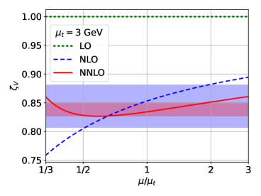
In order to see the improvement of the impact of the NNLO terms, we display in Fig. 4 the result for $\zeta_{\text{V}}$ as a function of the unphysical renormalization scale $\mu$ at leading order (LO), NLO, and NNLO. The flow-time $t$ has been fixed at $\mu_{t}=3$ GeV and $\mu_{t}=10$ GeV, corresponding to $t\approx 0.003$ GeV^-2 and $t=0.03$ GeV^-2, cf. Eq. 3.4. For the plot at $\mu_{t}=10$ GeV, we set $n_{\text{f}}=5$ and use $\alpha_{s}^{(n_{\text{f}}=5)}(10\,\text{GeV})=0.1880$ as input. For the plot at $\mu_{t}=3$ GeV, we set $n_{\text{f}}=3$ and use $\alpha_{s}^{(n_{\text{f}}=3)}(3\,\text{GeV})=0.2485$ as input. We then evaluate $\alpha_{s}(\mu)$ through one-, two-, and three-loop running for $\mu_{t}/3\leq\mu\leq 3\mu_{t}$ and insert it into the LO-, NLO-, and NNLO-approximation of $\zeta_{\text{V}}(t)$ (with the corresponding value for $n_{\text{f}}$) in order to obtain the three curves in the plots.

Figure 4: The matching coefficient $\zeta_{\text{V}}(t)$ at two different values of $t=e^{-\gamma_{\text{E}}}/(2\mu_{t}^{2})$ as a function of $\mu/\mu_{t}$.

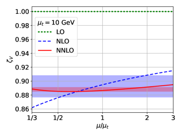Since this quantity is RG invariant, we expect the $\mu$ dependence to decrease from NLO to NNLO, and this is indeed what we observe. Taking the variation of $\mu$ around $\mu_{t}$ by a factor of two as an estimate of the perturbative uncertainty, we find that it decreases from 4.4% to 1.4% at $\mu_{t}=3$ GeV, and from 1.8% to 0.4% at 10 GeV. This is indicated by the red and blue bands in the plot. Another important observation is that these bands overlap, indicating that $\mu_{t}$ as defined in Eq. 3.4 is indeed a reasonable choice for the central renormalization scale. Since the other matching coefficients are not RG invariant, we refrain from showing the analogous plots for them.

4 Flowed anomalous dimension

As suggested in Ref. [33] for a general set of flowed operators $\mathcal{O}=(\mathcal{O}_{1},\ldots,\mathcal{O}_{p})$, one may define flowed anomalous dimensions which allow to resum their logarithmic $t$-dependence. Let us briefly recapitulate the idea behind it. First consider the flow time $t$ and the renormalization scale $\mu$ as independent quantities. The regular operators $\mathcal{O}$ are then independent of $t$, the flowed operators $\tilde{O}$ are independent of $\mu$, and the elements of the matching matrix $\zeta$ are functions of $a_{\text{s}}(\mu)$ and $L_{\mu t}$. Therefore, neglecting terms that vanish as $t\to 0$,

$$0=t\frac{\mathrm{d}}{\mathrm{d}t}\mathcal{O}=t\frac{\mathrm{d}}{\mathrm{d}t}\zeta^{-1}\,\tilde{\mathcal{O}}$$ (4.1)

and thus

$$t\frac{\mathrm{d}}{\mathrm{d}t}\tilde{\mathcal{O}}=\tilde{\gamma}\,\tilde{\mathcal{O}}\,,\quad\mbox{with}\quad\tilde{\gamma}=\left(t\frac{\mathrm{d}}{\mathrm{d}t}\zeta\right)\zeta^{-1}\,,$$ (4.2)

where the flowed anomalous dimension matrix $\tilde{\gamma}$ is a function of $a_{\text{s}}(\mu)$ and $L_{\mu t}$, which is, however, formally independent of $\mu$:

$$\mu^{2}\frac{\mathrm{d}}{\mathrm{d}\mu^{2}}\tilde{\gamma}=0\,.$$ (4.3)

Note that the derivative acting on $\zeta$ in Eq. 4.2 only affects the logarithmic terms $L_{\mu t}$. The latter can be derived at higher orders by noting that flowed operators (in the ringed scheme) are $\mu$-independent, i.e.

$$0=\mu^{2}\frac{\mathrm{d}}{\mathrm{d}\mu^{2}}\tilde{\mathcal{O}}=\mu^{2}\frac{\mathrm{d}}{\mathrm{d}\mu^{2}}\zeta\,\mathcal{O}=\left[\left(\frac{\partial}{\partial L_{\mu t}}+a_{\text{s}}\beta(a_{\text{s}})\frac{\partial}{\partial a_{\text{s}}}\right)\zeta\right]\mathcal{O}+\zeta\,\gamma\,\mathcal{O}\,,$$ (4.4)

where $\gamma$ is the anomalous dimension matrix of the regular operators $\mathcal{O}$, i.e. $\mu^{2}\frac{\mathrm{d}}{\mathrm{d}\mu^{2}}\mathcal{O}=\gamma\mathcal{O}$. Therefore,

$$\tilde{\gamma} =-\left(a_{\text{s}}\beta\frac{\partial}{\partial a_{\text{s}}}\zeta\right)\zeta^{-1}-\zeta\gamma\zeta^{-1}\,.$$ (4.5)

The term in brackets starts at ${\cal O}(a_{\text{s}}^{2})$, and thus the one-loop term of the flowed anomalous dimension is given by the (negative of the) regular anomalous dimension of the current. Furthermore, knowledge of $\zeta$ at order $a_{\text{s}}^{n}$ is sufficient to obtain $\tilde{\gamma}$ through order $a_{\text{s}}^{n+1}$, given that $\gamma$ is known to $a_{\text{s}}^{n+1}$ and $\beta$ to $a_{\text{s}}^{n}$.

It may be interesting to note that Eq. 4.5 can also be derived by tying the flow time and the renormalization scale together from the start, i.e., setting $\mu=c/\sqrt{t}$, with some constant $c$. In this case, also the regular operators become $t$ dependent, while $\zeta$ depends on $t$ only through $a_{\text{s}}(c/\sqrt{t})$, and thus

$$t\frac{\mathrm{d}}{\mathrm{d}t}\mathcal{O}=-\mu^{2}\frac{\mathrm{d}}{\mathrm{d}\mu^{2}}\mathcal{O}=-\gamma\mathcal{O}\quad\mbox{and}\quad t\frac{\mathrm{d}}{\mathrm{d}t}\zeta(t)=-a_{\text{s}}\beta\frac{\partial}{\partial a_{\text{s}}}\zeta(t)\,,$$ (4.6)

which again leads to

$$t\frac{\mathrm{d}}{\mathrm{d}t}\mathcal{O}=\left[-a_{\text{s}}\beta\frac{\partial}{\partial a_{\text{s}}}\zeta-\zeta\gamma\right]\zeta^{-1}\mathcal{O}\,.$$ (4.7)

Applied to the current operators considered in this paper, Eq. 4.2 reads

$$t\frac{\mathrm{d}}{\mathrm{d}t}\tilde{j}=\tilde{\gamma}\,\tilde{j}\,,$$ (4.8)

and using Eqs. 4.5, 3.8, 3.9, 3.10, A.16, and A.17, we find

$$\tilde{\gamma}_{\text{S}}(t) =-\frac{3}{4}a_{\text{s}}C_{\text{F}}+a_{\text{s}}^{2}\Bigg{[}-\frac{3}{32}C_{\text{F}}^{2}+C_{\text{A}}C_{\text{F}}\Big{(}-\frac{47}{32}-\frac{11}{12}\ln 2-\frac{11}{16}\ln 3\Big{)}$$

$$\hskip 20.00003pt+C_{\text{F}}T_{\text{R}}n_{\text{f}}\Big{(}\frac{3}{8}+\frac{1}{3}\ln 2+\frac{1}{4}\ln 3\Big{)}\Bigg{]}$$

$$\hskip 10.00002pt+a_{\text{s}}^{3}\Bigg{\{}\Big{(}\frac{11}{96}C_{\text{A}}-\frac{1}{24}T_{\text{R}}n_{\text{f}}\Big{)}c_{\chi}^{(2)}-\frac{129}{128}C_{\text{F}}^{3}+C_{\text{F}}^{2}C_{\text{A}}\Big{(}\frac{305}{256}+\frac{11}{12}\zeta_{2}-\frac{11}{3}\ln 2$$

$$\hskip 30.00005pt-\frac{11}{24}\ln^{2}2-\frac{11}{8}\ln 2\ln 3+\frac{33}{8}\ln 3-\frac{33}{64}\ln^{2}3+\frac{11}{2}\text{Li}_{2}\left(1/4\right)\Big{)}$$

$$\hskip 20.00003pt+C_{\text{F}}C_{\text{A}}^{2}\Big{(}-\frac{65869}{6912}-\frac{77}{96}\zeta_{2}-\frac{215}{24}\ln 2+\frac{11}{24}\ln^{2}2+\frac{247}{32}\ln 3+\frac{11}{4}\text{Li}_{2}\left(1/4\right)\Big{)}$$

$$\hskip 20.00003pt+C_{\text{F}}^{2}T_{\text{R}}n_{\text{f}}\Big{(}\frac{19}{32}-\frac{1}{3}\zeta_{2}+\frac{19}{12}\ln 2+\frac{1}{6}\ln^{2}2+\frac{1}{2}\ln 2\ln 3-\frac{21}{16}\ln 3+\frac{3}{16}\ln^{2}3$$

$$\hskip 30.00005pt-2\text{Li}_{2}\left(1/4\right)-\frac{3}{4}\zeta_{3}\Big{)}+C_{\text{F}}T_{\text{R}}^{2}n_{\text{f}}^{2}\Big{(}-\frac{205}{432}-\frac{1}{6}\zeta_{2}\Big{)}$$

$$\hskip 20.00003pt+C_{\text{F}}C_{\text{A}}T_{\text{R}}n_{\text{f}}\Big{(}\frac{2071}{432}+\frac{3}{4}\zeta_{2}+\frac{41}{12}\ln 2-\frac{1}{6}\ln^{2}2-\frac{43}{16}\ln 3$$

$$\hskip 30.00005pt-\text{Li}_{2}\left(1/4\right)+\frac{3}{4}\zeta_{3}\Big{)}\Bigg{\}}+\mathcal{O}(a_{\text{s}}^{4})\,,$$ (4.9)

$$\tilde{\gamma}_{\text{V}}(t) =a_{\text{s}}^{2}\Bigg{[}C_{\text{A}}C_{\text{F}}\Big{(}\frac{11}{96}-\frac{11}{12}\ln 2-\frac{11}{16}\ln 3\Big{)}+C_{\text{F}}T_{\text{R}}n_{\text{f}}\Big{(}-\frac{1}{24}+\frac{1}{3}\ln 2+\frac{1}{4}\ln 3\Big{)}\Bigg{]}$$

$$\hskip 10.00002pt+a_{\text{s}}^{3}\Bigg{\{}\Big{(}\frac{11}{96}C_{\text{A}}-\frac{1}{24}T_{\text{R}}n_{\text{f}}\Big{)}c_{\chi}^{(2)}+C_{\text{F}}^{2}C_{\text{A}}\Big{(}-\frac{77}{128}-\frac{55}{192}\zeta_{2}+\frac{11}{12}\ln 2$$

$$\hskip 30.00005pt-\frac{11}{24}\ln^{2}2-\frac{11}{8}\ln 2\ln 3-\frac{33}{64}\ln^{2}3+\frac{11}{4}\text{Li}_{2}\left(1/4\right)\Big{)}$$

$$\hskip 20.00003pt+C_{\text{F}}C_{\text{A}}^{2}\Big{(}-\frac{8189}{2304}-\frac{55}{192}\zeta_{2}-\frac{20}{3}\ln 2+\frac{11}{24}\ln^{2}2+\frac{181}{32}\ln 3+\frac{77}{32}\text{Li}_{2}\left(1/4\right)\Big{)}$$

$$\hskip 20.00003pt+C_{\text{F}}^{2}T_{\text{R}}n_{\text{f}}\Big{(}\frac{3}{16}+\frac{5}{48}\zeta_{2}-\frac{1}{12}\ln 2+\frac{1}{6}\ln^{2}2+\frac{1}{2}\ln 2\ln 3+\frac{3}{16}\ln 3$$

$$\hskip 30.00005pt+\frac{3}{16}\ln^{2}3-\text{Li}_{2}\left(1/4\right)\Big{)}+C_{\text{F}}T_{\text{R}}^{2}n_{\text{f}}^{2}\Big{(}-\frac{35}{144}-\frac{1}{12}\zeta_{2}\Big{)}$$

$$\hskip 20.00003pt+C_{\text{F}}C_{\text{A}}T_{\text{R}}n_{\text{f}}\Big{(}\frac{559}{288}+\frac{1}{3}\zeta_{2}+\frac{31}{12}\ln 2-\frac{1}{6}\ln^{2}2-\frac{31}{16}\ln 3-\frac{7}{8}\text{Li}_{2}\left(1/4\right)\Big{)}\Bigg{\}}$$

$$\hskip 10.00002pt+\mathcal{O}(a_{\text{s}}^{4})\,,$$ (4.10)

$$\tilde{\gamma}_{\text{T}}(t) =\frac{1}{4}a_{\text{s}}C_{\text{F}}+a_{\text{s}}^{2}\bigg{[}-\frac{19}{32}C_{\text{F}}^{2}+C_{\text{A}}C_{\text{F}}\Big{(}\frac{257}{288}-\frac{11}{12}\ln 2-\frac{11}{16}\ln 3\Big{)}$$

$$\hskip 20.00003pt+C_{\text{F}}T_{\text{R}}n_{\text{f}}\Big{(}-\frac{13}{72}+\frac{1}{3}\ln 2+\frac{1}{4}\ln 3\Big{)}\bigg{]}$$

$$\hskip 10.00002pt+a_{\text{s}}^{3}\Bigg{\{}\Big{(}\frac{11}{96}C_{\text{A}}-\frac{1}{24}T_{\text{R}}n_{\text{f}}\Big{)}c_{\chi}^{(2)}+C_{\text{F}}^{3}\Big{(}\frac{365}{384}-\zeta_{3}\Big{)}$$

$$\hskip 20.00003pt+C_{\text{F}}^{2}C_{\text{A}}\Big{(}-\frac{9287}{2304}-\frac{11}{24}\zeta_{2}+\frac{22}{9}\ln 2-\frac{11}{24}\ln^{2}2$$

$$\hskip 30.00005pt-\frac{11}{8}\ln 2\ln 3-\frac{11}{8}\ln 3-\frac{33}{64}\ln^{2}3+\frac{11}{6}\text{Li}_{2}\left(1/4\right)+\frac{7}{4}\zeta_{3}\Big{)}$$

$$\hskip 10.00002pt+C_{\text{F}}C_{\text{A}}^{2}\Big{(}-\frac{10079}{20736}-\frac{11}{96}\zeta_{2}-\frac{425}{72}\ln 2+\frac{11}{24}\ln^{2}2+\frac{159}{32}\ln 3$$

$$\hskip 30.00005pt+\frac{55}{24}\text{Li}_{2}\left(1/4\right)-\frac{5}{8}\zeta_{3}\Big{)}$$

$$\hskip 20.00003pt+C_{\text{F}}^{2}T_{\text{R}}n_{\text{f}}\Big{(}\frac{161}{288}+\frac{1}{6}\zeta_{2}-\frac{23}{36}\ln 2+\frac{1}{6}\ln^{2}2+\frac{1}{2}\ln 2\ln 3+\frac{11}{16}\ln 3+\frac{3}{16}\ln^{2}3$$

$$\hskip 30.00005pt-\frac{2}{3}\text{Li}_{2}\left(1/4\right)+\frac{1}{4}\zeta_{3}\Big{)}+C_{\text{F}}T_{\text{R}}^{2}n_{\text{f}}^{2}\Big{(}-\frac{215}{1296}-\frac{1}{18}\zeta_{2}\Big{)}$$

$$\hskip 20.00003pt+C_{\text{F}}C_{\text{A}}T_{\text{R}}n_{\text{f}}\Big{(}\frac{923}{1296}+\frac{7}{36}\zeta_{2}+\frac{83}{36}\ln 2-\frac{1}{6}\ln^{2}2-\frac{27}{16}\ln 3$$

$$\hskip 30.00005pt-\frac{5}{6}\text{Li}_{2}\left(1/4\right)-\frac{1}{4}\zeta_{3}\Big{)}\Bigg{\}}+\mathcal{O}(a_{\text{s}}^{4})\,,$$ (4.11)

$$\tilde{\gamma}_{\text{P}}(t) =\tilde{\gamma}_{\text{S}}(t)\,,$$ (4.12)

$$\tilde{\gamma}_{\text{A}}^{\text{ns}}(t) =\tilde{\gamma}_{\text{V}}(t)\,,$$ (4.13)

$$\tilde{\gamma}^{\text{s}}_{\text{A}}(t) =\tilde{\gamma}^{\text{ns}}_{\text{A}}(t)+\frac{3}{4}a_{\text{s}}^{2}C_{\text{F}}T_{\text{R}}n_{\text{f}}+a_{\text{s}}^{3}\bigg{[}-\frac{9}{16}C_{\text{F}}^{2}T_{\text{R}}n_{\text{f}}$$

$$\hskip 20.00003pt+C_{\text{F}}T_{\text{R}}^{2}n_{\text{f}}^{2}\Big{(}\frac{1}{6}-\frac{1}{12}\zeta_{2}-3\ln 2+\frac{3}{2}\ln 3-\frac{5}{4}\text{Li}_{2}\left(1/4\right)\Big{)}$$

$$\hskip 20.00003pt+C_{\text{F}}C_{\text{A}}T_{\text{R}}n_{\text{f}}\Big{(}\frac{19}{24}+\frac{11}{48}\zeta_{2}+\frac{33}{4}\ln 2-\frac{33}{8}\ln 3+\frac{55}{16}\text{Li}_{2}\left(1/4\right)\Big{)}\bigg{]}$$

$$\hskip 10.00002pt+\mathcal{O}(a_{\text{s}}^{4})\,.$$ (4.14)

Note that, in these formulas, $a_{\text{s}}$ is still renormalized in the $\overline{\mathrm{{MS}}}$ scheme, and we have set $\mu=\mu_{t}$, see Eq. 3.4 (the expression for general $\mu$ can be easily reconstructed using Eq. 4.3; it is also given in the ancillary file accompanying this paper, see Appendix B). In order to eliminate any reference to the $\overline{\mathrm{{MS}}}$ scheme, one can simply convert $a_{\text{s}}$ in these expressions to the gradient-flow scheme according to [3]

$$a_{\text{s}}=\hat{a}_{\text{s}}\left[1-e_{1}\hat{a}_{\text{s}}+\hat{a}_{\text{s}}^{2}(2e_{1}^{2}-e_{2})+{\cal O}(\hat{a}_{\text{s}}^{3})\ldots\right]\,,$$ (4.15)

where

$$\begin{split}e_{0}&=e_{00}\,,\qquad e_{1}=e_{10}+\beta_{0}\,L_{\mu t}\,,\\ e_{2}&=e_{20}+(2\beta_{0}\,e_{10}+\beta_{1})\,L_{\mu t}+\beta_{0}^{2}\,L_{\mu t}^{2}\,,\end{split}$$ (4.16)

with $\beta_{0}$, $\beta_{1}$ from Eq. A.4, and [3, 59, 28]

$$\begin{split}e_{00}&=1\,,\qquad e_{10}=\left(\frac{13}{9}+\frac{11}{6}\ln 2-\frac{3}{4}\ln 3\right)C_{\text{A}}-\frac{2}{9}T_{\text{R}}n_{\text{f}}\,,\\ e_{20}&=1.74865\,C_{\text{A}}^{2}-(1.97283\ldots)\,C_{\text{A}}T_{\text{R}}n_{\text{f}}+\left(\zeta_{3}-\frac{43}{48}\right)C_{\text{F}}T_{\text{R}}n_{\text{f}}\\ &\hskip 10.00002pt+\left(\frac{1}{9}\zeta_{2}-\frac{5}{81}\right)T_{\text{R}}^{2}n_{\text{f}}^{2}\,.\end{split}$$ (4.17)

The exact expression for the coefficient of $C_{\text{A}}T_{\text{R}}n_{\text{f}}$ can be found in Ref. [28].

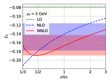
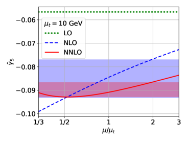
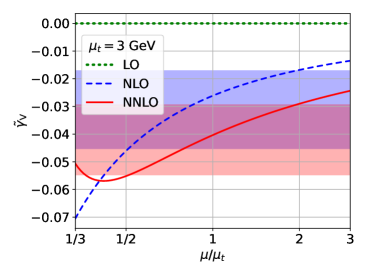
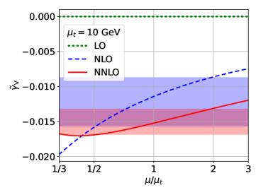
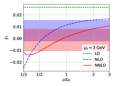
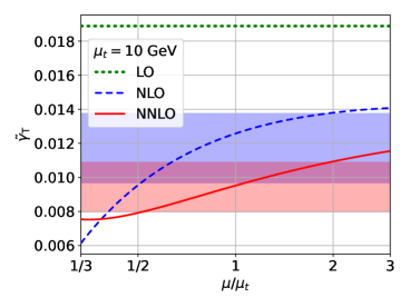
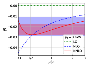
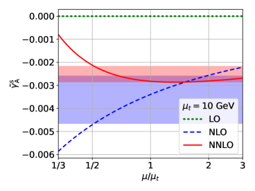
Numerical values for the flowed anomalous dimensions are shown in Fig. 5. The input parameters are the same as in Fig. 4. Also here, we observe the expected reduction of the renormalization scale dependence when including higher orders, albeit sometimes less pronounced than for $\zeta_{\text{V}}(t)$. But also here the NLO and the NNLO uncertainty bands nicely overlap.

Figure 5: The flowed anomalous dimensions at two different values of $t=e^{-\gamma_{\text{E}}}/(2\mu_{t}^{2})$ as functions of $\mu/\mu_{t}$.

5 Conclusions

In this paper, we have considered the SFTX of the scalar, pseudoscalar, vector, axialvector, and tensor currents and computed the corresponding matching coefficients through NNLO in QCD. Possible applications of these results are the calculation of the chiral condensate on the lattice [19] or the semileptonic contributions to the neutron electric dipole moment [37].

Our results could also serve as alternatives to the ringed renormalization scheme [13], which requires the calculation of the vacuum expectation value of the quark kinetic operator. In certain cases, it may be more efficient to normalize quark matrix elements to one of the currents instead. We believe that this strategy will especially find applications in flavor physics, in particular in combination with the SFTX of the relevant four-quark operators [29, 31]. A first preliminary study, already employing the result for the axialvector current obtained in the present paper, has been published in Ref. [34].

Finally, the simplicity of the quark currents could also be advantageous for systematic studies of the SFTX, building up on the preliminary studies of Refs. [26, 35, 36] in different contexts.

Acknowledgments.

We thank Matthew Black, Mattia Dalla Brida, Antonio Rago, Andrea Shindler, and Oliver Witzel for motivation of this project, helpful discussions, and comments on the manuscript.

This research was supported by the Deutsche Forschungsgemeinschaft (DFG, German Research Foundation) under grant 396021762 - TRR 257. The work of F.L. was supported by the Swiss National Science Foundation (SNSF) under contract TMSGI2_211209.

Appendix A Renormalization constants

In this appendix, we collect the renormalization constants required to arrive at the finite results presented in this paper. Most of these constants are known to higher loop orders, but we will display only the orders which are relevant for our calculation.

The relation between the bare and $\overline{\mathrm{{MS}}}$-renormalized gauge coupling is given by the regular-QCD expression

$$g_{\text{{B}}}=\left(\frac{\mu^{2}e^{\gamma_{\text{E}}}}{4\pi}\right)^{\epsilon/2}Z_{g}(a_{\text{s}}(\mu))g(\mu)\,,$$ (A.1)

with $\mu$ the renormalization scale, $\gamma_{\text{E}}=0.577215\ldots$ the Euler-Mascheroni constant,

$$Z_{g}(a_{\text{s}}) =1-a_{\text{s}}\frac{\beta_{0}}{2\epsilon}+a_{\text{s}}^{2}\left(\frac{3\beta_{0}^{2}}{8\epsilon^{2}}-\frac{\beta_{1}}{4\epsilon}\right)+\mathcal{O}(a_{\text{s}}^{3})\,,$$ (A.2)

$a_{\text{s}}$ from Eq. 3.5, and the coefficients of the QCD beta function

$$\beta(a_{\text{s}})=-\epsilon-a_{\text{s}}\sum_{n=0}^{\infty}\beta_{n}a_{\text{s}}^{n}\,,$$ (A.3)

given by

$$\beta_{0} =\frac{1}{4}\left(\frac{11}{3}C_{\text{A}}-\frac{4}{3}T_{\text{R}}n_{\text{f}}\right)\,, \beta_{1} =\frac{1}{16}\left[\frac{34}{3}C_{\text{A}}^{2}-\left(4C_{\text{F}}+\frac{20}{3}C_{\text{A}}\right)T_{\text{R}}n_{\text{f}}\right]\,.$$ (A.4)

The QCD color factors are defined in Eq. 3.3, and $n_{\text{f}}$ is the number of quark flavors. The remaining $\overline{\mathrm{{MS}}}$ renormalization constants are cast into the generic form

$$Z^{\overline{\mathrm{{MS}}}}(a_{\text{s}}) =1-a_{\text{s}}\,\frac{\gamma_{0}}{\epsilon}+a_{\text{s}}^{2}\left[\frac{1}{2\epsilon^{2}}\left(\gamma^{2}_{0}+\beta_{0}\gamma_{0}\right)-\frac{\gamma_{1}}{2\epsilon}\right]+\mathcal{O}(a_{\text{s}}^{3})\,,$$ (A.5)

where the $\gamma_{n}$ are the perturbative coefficients of the corresponding anomalous dimensions. For the quark mass, the latter is defined as

$$\gamma_{m}(a_{\text{s}})=-a_{\text{s}}\sum_{n\geq 0}a_{\text{s}}^{n}\gamma_{m,n}\equiv-a_{\text{s}}\beta(a_{\text{s}})\frac{\mathrm{d}}{\mathrm{d}a_{\text{s}}}\ln Z_{m}^{\overline{\mathrm{{MS}}}}(a_{\text{s}})\,,$$ (A.6)

and thus

$$\mu^{2}\frac{\mathrm{d}}{\mathrm{d}\mu^{2}}m(\mu)=\gamma_{m}(a_{\text{s}})m(\mu)\,.$$ (A.7)

For the current $j$, we define

$$\gamma(a_{\text{s}})=a_{\text{s}}\sum_{n\geq 0}a_{\text{s}}^{n}\gamma_{n}\equiv a_{\text{s}}\beta(a_{\text{s}})\frac{\mathrm{d}}{\mathrm{d}a_{\text{s}}}\ln Z^{\overline{\mathrm{{MS}}}}(a_{\text{s}})\,.$$ (A.8)

The renormalization group equation for the currents is thus given by

$$\mu^{2}\frac{\mathrm{d}}{\mathrm{d}\mu^{2}}j(\mu)=\left[\gamma(a_{\text{s}})+\gamma^{\text{fin}}(a_{\text{s}})\right]j(\mu)\,,$$ (A.9)

where $\gamma^{\text{fin}}$ arises from any finite renormalization as introduced for the parity-odd currents when adopting Eq. 2.23. Specifically, if

$$Z(a_{\text{s}})=Z^{\text{fin}}(a_{\text{s}})\,Z^{\overline{\mathrm{{MS}}}}(a_{\text{s}})\,,\quad\text{with}\quad Z^{\text{fin}}(a_{\text{s}}) =1+\sum_{n=1}^{\infty}a_{\text{s}}^{n}z_{n0}\,,$$ (A.10)

then

$$\gamma^{\text{fin}}(a_{\text{s}}) =-a_{\text{s}}^{2}\,\beta_{0}\,z_{10}-a_{\text{s}}^{3}\bigg{[}\beta_{1}\,z_{10}-\beta_{0}\,z_{10}^{2}+2\beta_{0}\,z_{20}\bigg{]}+{\cal O}(a_{\text{s}}^{4})\,.$$ (A.11)

In this paper, we need the $\overline{\mathrm{{MS}}}$ quark mass renormalization constant $Z_{m}\equiv Z_{m}^{\overline{\mathrm{{MS}}}}$ through ${\cal O}(a_{\text{s}}^{3})$, given by

$$\gamma_{m,0} =\frac{3}{4}C_{\text{F}}\,,\qquad\gamma_{m,1}=\frac{3}{32}C_{\text{F}}^{2}+\frac{97}{96}C_{\text{A}}C_{\text{F}}-\frac{5}{24}C_{\text{F}}T_{\text{R}}n_{\text{f}}\,,$$ (A.12)

$$\gamma_{m,2} =\frac{1}{64}\bigg{[}\frac{129}{2}C_{\text{F}}^{3}-\frac{129}{4}C_{\text{F}}^{2}C_{\text{A}}+\frac{11413}{108}C_{\text{F}}C_{\text{A}}^{2}$$

$$+C_{\text{F}}^{2}T_{\text{R}}n_{\text{f}}\left(-46+48\zeta_{3}\right)+C_{\text{F}}C_{\text{A}}T_{\text{R}}n_{\text{f}}\left(-\frac{556}{27}-48\zeta_{3}\right)-\frac{140}{27}C_{\text{F}}T_{\text{R}}^{2}n_{\text{f}}^{2}\bigg{]}\,,$$

as well as the renormalization constant of the vacuum energy $Z_{0}$ through $\mathcal{O}(a_{\text{s}}^{2})$. It is related to the corresponding anomalous dimension $\gamma_{0}$ through

$$\gamma_{0}(a_{\text{s}})=\left[4\gamma_{m}(a_{\text{s}})-\epsilon\right]Z_{0}(a_{\text{s}})+\beta(a_{\text{s}})a_{\text{s}}\frac{\partial}{\partial a_{\text{s}}}Z_{0}(a_{\text{s}})\equiv-\frac{n_{\text{c}}n_{\text{h}}}{(4\pi)^{2}}\sum_{n\geq 0}a_{\text{s}}^{n}\gamma_{0,n}\,,$$ (A.13)

which leads to

$$Z_{0}(a_{\text{s}})=\frac{n_{\text{c}}n_{\text{h}}}{(4\pi)^{2}\epsilon}\Bigg{\{}1+a_{\text{s}} \left(\frac{\gamma_{0,1}}{2}-\frac{2\gamma_{m,0}}{\epsilon}\right)+a_{\text{s}}^{2}\Bigg{[}\frac{2}{3\epsilon^{2}}(\beta_{0}\gamma_{m,0}+4\gamma_{m,0}^{2})$$ (A.14)

$$-\frac{1}{6\epsilon}(\beta_{0}\gamma_{0,1}+4\gamma_{0,1}\gamma_{m,0}+8\gamma_{m,1})+\frac{1}{3}\gamma_{0,2}\Bigg{]}\Bigg{\}}+\mathcal{O}(a_{\text{s}}^{3})\,.$$

The first three perturbative coefficients are given by [60, 61]

$$\gamma_{0,0}=1\,,\qquad\gamma_{0,1}=C_{\text{F}}\,,$$ (A.15)

$$\gamma_{0,2}=-C_{\text{F}}^{2}\left(\frac{131}{32}-3\zeta_{3}\right)-C_{\text{F}}C_{\text{A}}\left(-\frac{109}{32}+\frac{3}{2}\zeta_{3}\right)-C_{\text{F}}T_{\text{R}}\left(\frac{5}{8}n_{\text{f}}+3n_{\text{h}}\right)\,.$$

The current renormalizations $Z^{\overline{\mathrm{{MS}}}}_{\mathrm{T}}$, $Z^{\overline{\mathrm{{MS}}}}_{\mathrm{P}}$, and $Z^{\overline{\mathrm{{MS}}}}_{\mathrm{A}}$ are needed through ${\cal O}(a_{\text{s}}^{2})$. For these [62, 43, 42],

$$\gamma_{\text{T},0} =-\frac{1}{4}C_{\text{F}}\,,\qquad \gamma_{\text{T},1} =\frac{19}{32}C_{\text{F}}^{2}-\frac{257}{288}C_{\text{A}}C_{\text{F}}+\frac{13}{72}C_{\text{F}}T_{\text{R}}n_{\text{f}}\,,$$ (A.16)

$$\gamma_{\text{P},0} =\frac{3}{4}C_{\text{F}}\,,\qquad \gamma_{\text{P},1} =\frac{3}{32}C_{\text{F}}^{2}-\frac{79}{96}C_{\text{A}}C_{\text{F}}+\frac{11}{24}C_{\text{F}}T_{\text{R}}n_{\text{f}}\,,$$

$$\gamma^{\text{ns}}_{\text{A},0} =0\,,\qquad \gamma^{\text{ns}}_{\text{A},1} =-\frac{11}{12}C_{\text{A}}C_{\text{F}}+\frac{1}{3}C_{\text{F}}T_{\text{R}}n_{\text{f}}\,,$$

$$\gamma^{\text{s}}_{\text{A},0} =0\,,\qquad \gamma^{\text{s}}_{\text{A},1} =\gamma^{\text{ns}}_{\text{A},1}-\frac{3}{4}C_{\text{F}}T_{\text{R}}n_{\text{f}}\,.$$

In order to derive the $\mathcal{O}(a_{\text{s}}^{3})$ terms of $\tilde{\gamma}$ in Section 4, we also need the terms at ${\cal O}(a_{\text{s}}^{3})$ [63, 43, 42]:

$$\gamma_{\text{T},2} =\left(\zeta_{3}-\frac{365}{384}\right)C_{\text{F}}^{3}+\left(\frac{6823}{2304}-\frac{7}{4}\zeta_{3}\right)C_{\text{F}}^{2}C_{\text{A}}+\left(\frac{5}{8}\zeta_{3}-\frac{13639}{6912}\right)C_{\text{F}}C_{\text{A}}^{2}$$ (A.17)

$$\hskip 10.00002pt-\left(\frac{49}{288}+\frac{1}{4}\zeta_{3}\right)C_{\text{F}}^{2}T_{\text{R}}n_{\text{f}}+\frac{1}{48}C_{\text{F}}T_{\text{R}}^{2}n_{\text{f}}^{2}+\left(\frac{251}{432}+\frac{1}{4}\zeta_{3}\right)C_{\text{F}}C_{\text{A}}T_{\text{R}}n_{\text{f}}\,,$$

$$\gamma_{\text{P},2} =\frac{599}{2304}C_{\text{A}}^{2}C_{\text{F}}-\frac{3203}{768}C_{\text{A}}C_{\text{F}}^{2}+\frac{129}{128}C_{\text{F}}^{3}+\frac{29}{48}C_{\text{A}}C_{\text{F}}n_{\text{f}}T_{\text{R}}+\frac{107}{96}C_{\text{F}}^{2}n_{\text{f}}T_{\text{R}}$$

$$\hskip 10.00002pt-\frac{17}{144}C_{\text{F}}T_{\text{R}}^{2}n_{\text{f}}^{2}-\frac{3}{4}\zeta_{3}C_{\text{A}}C_{\text{F}}T_{\text{R}}n_{\text{f}}+\frac{3}{4}\zeta_{3}C_{\text{F}}^{2}T_{\text{R}}n_{\text{f}}\,,$$

$$\gamma^{\text{ns}}_{\text{A},2} =\frac{77}{48}C_{\text{F}}^{2}C_{\text{A}}-\frac{1789}{864}C_{\text{F}}C_{\text{A}}^{2}-\frac{1}{3}C_{\text{F}}^{2}T_{\text{R}}n_{\text{f}}-\frac{1}{54}C_{\text{F}}T_{\text{R}}^{2}n_{\text{f}}^{2}+\frac{26}{27}C_{\text{F}}C_{\text{A}}T_{\text{R}}n_{\text{f}}\,,$$

$$\gamma^{\text{s}}_{\text{A},2} =\gamma^{\text{ns}}_{\text{A},2}+\frac{9}{16}C_{\text{F}}^{2}T_{\text{R}}n_{\text{f}}-\frac{1}{24}C_{\text{F}}T_{\text{R}}^{2}n_{\text{f}}^{2}-\frac{109}{96}C_{\text{F}}C_{\text{A}}T_{\text{R}}n_{\text{f}}\,.$$

Recall that the vector current does not require renormalization, and the scalar current renormalizes with $Z_{\text{S}}\equiv Z_{m}$. The finite renormalization constants for the axial and the pseudoscalar current introduced in Eq. 3.11 are given by [43, 42]

$$Z_{5,\text{P}}(a_{\text{s}}) =1-2\,a_{\text{s}}C_{\text{F}}+a_{\text{s}}^{2}\Big{(}\frac{1}{72}C_{\text{F}}C_{\text{A}}+\frac{1}{18}C_{\text{F}}T_{\text{R}}n_{\text{f}}\Big{)}+\mathcal{O}(a_{\text{s}}^{3})\,,$$ (A.18)

$$Z^{\text{ns}}_{5,\text{A}}(a_{\text{s}}) =1-a_{\text{s}}C_{\text{F}}+a_{\text{s}}^{2}\left(\frac{11}{8}C_{\text{F}}^{2}-\frac{107}{144}C_{\text{F}}C_{\text{A}}+\frac{1}{36}C_{\text{F}}T_{\text{R}}n_{\text{f}}\right)+\mathcal{O}(a_{\text{s}}^{3})\,,$$

$$Z^{\text{s}}_{\text{5,A}}(a_{\text{s}}) =Z^{\text{ns}}_{\text{5,A}}+\frac{3}{16}a_{\text{s}}^{2}\,C_{\text{F}}T_{\text{R}}n_{\text{f}}+{\cal O}(a_{\text{s}}^{3})\,.$$

Let us remark that quoting the results for $Z^{\text{ns}}_{5,\text{A}}$ and $Z_{5,\text{P}}$ is redundant, because they could be derived from Eq. A.11 and

$$\gamma_{\text{S}} =\gamma_{\text{P}}+\gamma_{\text{P}}^{\text{fin}}\,,\qquad\gamma_{\text{V}}=\gamma_{\text{A}}^{\text{ns}}+\gamma_{\text{A}}^{\text{ns,fin}}\,.$$ (A.19)

The flowed-quark field renormalization constant introduced in Eq. 2.7 assumes the same form as Eq. A.5 with the anomalous dimensions given by [15, 17]

$$\gamma_{\chi,0} =-\frac{3}{4}C_{\text{F}}\,, \gamma_{\chi,1} =\left(\frac{1}{2}\ln 2-\frac{223}{96}\right)C_{\text{A}}C_{\text{F}}+\left(\frac{3}{32}+\frac{1}{2}\ln 2\right)C_{\text{F}}^{2}+\frac{11}{24}C_{\text{F}}T_{\text{R}}n_{\text{f}}\,.$$ (A.20)

Besides the $\overline{\mathrm{{MS}}}$ scheme, the so-called ringed scheme is determined from the all-order condition [13]

$$\mathring{Z}_{\chi}\langle\bar{\chi}_{p}(t)\overleftrightarrow{\not{\mathcal{D}}}^{\text{F}}\chi_{p}(t)\rangle\bigg{|}_{m=0}\equiv-\frac{2n_{\text{c}}n_{\text{f}}}{(4\pi t)^{2}}\,.$$ (A.21)

It is related to the $\overline{\mathrm{{MS}}}$ scheme by

$$\mathring{Z}_{\chi} =\zeta_{\chi}(t,\mu)Z^{\overline{\mathrm{{MS}}}}_{\chi}\,,$$ (A.22)

with the finite renormalization constant [13, 28]

$$\zeta_{\chi}(t,\mu)=1 -a_{\text{s}}\left(\gamma_{\chi,0}L_{\mu t}+\frac{3}{4}C_{\text{F}}\ln 3+C_{\text{F}}\ln 2\right)$$ (A.23)

$$+a_{\text{s}}^{2}\Bigg{\{}\frac{\gamma_{\chi,0}}{2}\left(\gamma_{\chi,0}-\beta_{0}\right)L_{\mu t}^{2}+\Big{[}\gamma_{\chi,0}\left(\beta_{0}-\gamma_{\chi,0}\right)\ln 3$$

$$+\frac{4}{3}\gamma_{\chi,0}\left(\beta_{0}-\gamma_{\chi,0}\right)\ln 2-\gamma_{\chi,1}\Big{]}L_{\mu t}+\frac{c_{\chi}^{(2)}}{16}\Bigg{\}}+\mathcal{O}(a_{\text{s}}^{3})\,,$$

where

$$c_{\chi}^{(2)} =C_{\text{A}}C_{\text{F}}\,c_{\chi,\text{A}}+C_{\text{F}}^{2}\,c_{\chi,\text{F}}+C_{\text{F}}T_{\text{R}}n_{\text{f}}\,c_{\chi,\text{R}}\,.$$ (A.24)

The coefficients have been evaluated in Ref. [28]:

$$c_{\chi,\text{A}} =-23.7947,\qquad c_{\chi,\text{F}}=30.3914,\qquad$$ (A.25)

$$c_{\chi,\text{R}} =-\frac{131}{18}+\frac{46}{3}\zeta_{2}+\frac{944}{9}\ln 2+\frac{160}{3}\ln^{2}2-\frac{172}{3}\ln 3+\frac{104}{3}\ln 2\ln 3$$

$$-\frac{178}{3}\ln^{2}3+\frac{8}{3}\text{Li}_{2}(1/9)-\frac{400}{3}\text{Li}_{2}(1/3)+\frac{112}{3}\text{Li}_{2}(3/4)=-3.92255\ldots\,.$$

Only digits are quoted in Eq. A.25 which are not affected by the numerical uncertainty.

Appendix B Ancillary file

For the reader’s convenience, we provide the main results of this paper as an ancillary file in Mathematica format. The results are encoded in the expressions listed in Table 1. The matching coefficients $\zeta$ are provided both in the ringed scheme of the fermions as well as in the $\overline{\mathrm{{MS}}}$ scheme. One may switch between the two schemes by setting the variable Xzetachi to 0 ($\overline{\mathrm{{MS}}}$ scheme) or 1 (ringed scheme). The flowed anomalous dimensions $\tilde{\gamma}$ are provided only in the ringed scheme.

The results depend on the variables listed in Table 2. The matching coefficients in the ringed scheme also contain the symbol C2, which corresponds to the coefficient $c_{\chi}^{(2)}$, defined in Eqs. A.24 and A.25. The latter relations are provided in the form of a Mathematica replacement rule named ReplaceC2.

Table 1: The expressions of the ancillary file that encode the main results of this paper.

expression	meaning	reference
zetaS1	$\zeta_{\text{S}}^{(1)}$	Eq. 3.6
zetaS3	$\zeta_{\text{S}}^{(3)}$	Eq. 3.7
zetaS	$\zeta_{\text{S}}$	Eq. 3.8
zetaV	$\zeta_{\text{V}}$	Eq. 3.9
zetaT	$\zeta_{\text{T}}$	Eq. 3.10
zetaAns	$\zeta_{\text{A}}^{\text{ns}}$	Eq. 3.12
zetaP	$\zeta_{\text{P}}$	Eq. 3.12
zetaAtriangle	$\zeta_{\text{A}}^{\Delta}$	Eq. 3.13
tildegammaS	$\tilde{\gamma}_{\text{S}}$	Eq. 4.9
tildegammaV	$\tilde{\gamma}_{\text{V}}$	Eq. 4.10
tildegammaT	$\tilde{\gamma}_{\text{T}}$	Eq. 4.11
tildegammaAns	$\tilde{\gamma}_{\text{A}}^{\text{ns}}$	Eq. 4.13
tildegammaAs	$\tilde{\gamma}_{\text{A}}^{\text{s}}$	Eq. 4.14
tildegammaP	$\tilde{\gamma}_{\text{P}}$	Eq. 4.12

Table 2: Notation for the variables in the ancillary file.

symbol	meaning	reference
nc	$n_{\text{c}}$	Eq. 3.3
tr	$T_{\text{R}}$	Eq. 3.3
cf	$C_{\text{F}}$	Eq. 3.3
ca	$C_{\text{A}}$	Eq. 3.3
Lmut	$L_{\mu t}$	Eq. 3.4
as	$a_{\text{s}}$	Eq. 3.5
nf	$n_{\text{f}}$	Section 2.2
nl	$n_{\text{l}}$	Section 2.2
nh	$n_{\text{h}}$	Section 2.2

References

- [1] R. Narayanan and H. Neuberger, “Infinite phase transitions in continuum Wilson loop operators”, JHEP 03 (2006) 064, arXiv:hep-th/0601210.
- [2] M. Lüscher, “Trivializing maps, the Wilson flow and the HMC algorithm”, Commun. Math. Phys. 293 (2010) 899–919, arXiv:0907.5491 [hep-lat].
- [3] M. Lüscher, “Properties and uses of the Wilson flow in lattice QCD”, JHEP 08 (2010) 071, arXiv:1006.4518 [hep-lat]. [Erratum: JHEP 03, 092 (2014)].
- [4] Budapest-Marseille-Wuppertal Collaboration, S. Borsányi et al., “High-precision scale setting in lattice QCD”, JHEP 09 (2012) 010, arXiv:1203.4469 [hep-lat].
- [5] Z. Fodor, K. Holland, J. Kuti, D. Nogradi, and C. H. Wong, “The Yang-Mills gradient flow in finite volume”, JHEP 11 (2012) 007, arXiv:1208.1051 [hep-lat].
- [6] P. Fritzsch and A. Ramos, “The gradient flow coupling in the Schrödinger functional”, JHEP 10 (2013) 008, arXiv:1301.4388 [hep-lat].
- [7] ALPHA Collaboration, M. Dalla Brida, P. Fritzsch, T. Korzec, A. Ramos, S. Sint, and R. Sommer, “Slow running of the gradient flow coupling from 200 MeV to 4 GeV in QCD”, Phys. Rev. D 95 (2017) 014507, arXiv:1607.06423 [hep-lat].
- [8] M. Dalla Brida and M. Lüscher, “SMD-based numerical stochastic perturbation theory”, Eur. Phys. J. C 77 (2017) 308, arXiv:1703.04396 [hep-lat].
- [9] Z. Fodor, K. Holland, J. Kuti, D. Nogradi, and C. H. Wong, “A new method for the beta function in the chiral symmetry broken phase”, EPJ Web Conf. 175 (2018) 08027, arXiv:1711.04833 [hep-lat].
- [10] A. Hasenfratz and O. Witzel, “Continuous renormalization group function from lattice simulations”, Phys. Rev. D 101 (2020) 034514, arXiv:1910.06408 [hep-lat].
- [11] M. Lüscher and P. Weisz, “Perturbative analysis of the gradient flow in non-abelian gauge theories”, JHEP 02 (2011) 051, arXiv:1101.0963 [hep-th].
- [12] H. Suzuki, “Energy–momentum tensor from the Yang–Mills gradient flow”, PTEP 2013 (2013) 083B03, arXiv:1304.0533 [hep-lat]. [Erratum: PTEP 2015 (2015) 079201].
- [13] H. Makino and H. Suzuki, “Lattice energy–momentum tensor from the Yang–Mills gradient flow—inclusion of fermion fields”, PTEP 2014 (2014) 063B02, arXiv:1403.4772 [hep-lat]. [Erratum: PTEP 2015 (2015) 079202].
- [14] C. Monahan and K. Orginos, “Locally smeared operator product expansions in scalar field theory”, Phys. Rev. D 91 (2015) 074513, arXiv:1501.05348 [hep-lat].
- [15] M. Lüscher, “Chiral symmetry and the Yang–Mills gradient flow”, JHEP 04 (2013) 123, arXiv:1302.5246 [hep-lat].
- [16] K. Hieda, H. Makino, and H. Suzuki, “Proof of the renormalizability of the gradient flow”, Nucl. Phys. B 918 (2017) 23–51, arXiv:1604.06200 [hep-lat].
- [17] R. V. Harlander, Y. Kluth, and F. Lange, “The two-loop energy–momentum tensor within the gradient-flow formalism”, Eur. Phys. J. C 78 (2018) 944, arXiv:1808.09837 [hep-lat]. [Erratum: Eur. Phys. J. C 79 (2019) 858].
- [18] FlowQCD Collaboration, M. Asakawa, T. Hatsuda, E. Itou, M. Kitazawa, and H. Suzuki, “Thermodynamics of SU(3) gauge theory from gradient flow on the lattice”, Phys. Rev. D 90 (2014) 011501, arXiv:1312.7492 [hep-lat]. [Erratum: Phys. Rev. D 92 (2015) 059902].
- [19] WHOT-QCD Collaboration, Y. Taniguchi, S. Ejiri, R. Iwami, K. Kanaya, M. Kitazawa, H. Suzuki, T. Umeda, and N. Wakabayashi, “Exploring = 2+1 QCD thermodynamics from the gradient flow”, Phys. Rev. D 96 (2017) 014509, arXiv:1609.01417 [hep-lat]. [Erratum: Phys. Rev. D 99 (2019) 059904].
- [20] M. Kitazawa, T. Iritani, M. Asakawa, T. Hatsuda, and H. Suzuki, “Equation of state for SU(3) gauge theory via the energy-momentum tensor under gradient flow”, Phys. Rev. D 94 (2016) 114512, arXiv:1610.07810 [hep-lat].
- [21] M. Kitazawa, T. Iritani, M. Asakawa, and T. Hatsuda, “Correlations of the energy-momentum tensor via gradient flow in SU(3) Yang-Mills theory at finite temperature”, Phys. Rev. D 96 (2017) 111502, arXiv:1708.01415 [hep-lat].
- [22] R. Yanagihara, T. Iritani, M. Kitazawa, M. Asakawa, and T. Hatsuda, “Distribution of stress tensor around static quark–anti-quark from Yang-Mills gradient flow”, Phys. Lett. B 789 (2019) 210–214, arXiv:1803.05656 [hep-lat].
- [23] T. Iritani, M. Kitazawa, H. Suzuki, and H. Takaura, “Thermodynamics in quenched QCD: energy–momentum tensor with two-loop order coefficients in the gradient-flow formalism”, PTEP 2019 (2019) 023B02, arXiv:1812.06444 [hep-lat].
- [24] WHOT-QCD Collaboration, Y. Taniguchi, S. Ejiri, K. Kanaya, M. Kitazawa, H. Suzuki, and T. Umeda, “ = 2+1 QCD thermodynamics with gradient flow using two-loop matching coefficients”, Phys. Rev. D 102 (2020) 014510, arXiv:2005.00251 [hep-lat]. [Erratum: Phys. Rev. D 102 (2020) 059903].
- [25] WHOT-QCD Collaboration, M. Shirogane, S. Ejiri, R. Iwami, K. Kanaya, M. Kitazawa, H. Suzuki, Y. Taniguchi, and T. Umeda, “Latent heat and pressure gap at the first-order deconfining phase transition of SU(3) Yang-Mills theory using the small flow-time expansion method”, PTEP 2021 (2021) 013B08, arXiv:2011.10292 [hep-lat].
- [26] H. Suzuki and H. Takaura, “ extrapolation function in the small flow time expansion method for the energy–momentum tensor”, PTEP 2021 (2021) 073B02, arXiv:2102.02174 [hep-lat].
- [27] L. Altenkort, A. M. Eller, A. Francis, O. Kaczmarek, L. Mazur, G. D. Moore, and H.-T. Shu, “Viscosity of pure-glue QCD from the lattice”, Phys. Rev. D 108 (2023) 014503, arXiv:2211.08230 [hep-lat].
- [28] J. Artz, R. V. Harlander, F. Lange, T. Neumann, and M. Prausa, “Results and techniques for higher order calculations within the gradient-flow formalism”, JHEP 06 (2019) 121, arXiv:1905.00882 [hep-lat]. [Erratum: JHEP 10 (2019) 032].
- [29] A. Suzuki, Y. Taniguchi, H. Suzuki, and K. Kanaya, “Four quark operators for kaon bag parameter with gradient flow”, Phys. Rev. D 102 (2020) 034508, arXiv:2006.06999 [hep-lat].
- [30] E. Mereghetti, C. J. Monahan, M. D. Rizik, A. Shindler, and P. Stoffer, “One-loop matching for quark dipole operators in a gradient-flow scheme”, JHEP 04 (2022) 050, arXiv:2111.11449 [hep-lat].
- [31] R. V. Harlander and F. Lange, “Effective electroweak Hamiltonian in the gradient-flow formalism”, Phys. Rev. D 105 (2022) L071504, arXiv:2201.08618 [hep-lat].
- [32] J. Borgulat, M. D. Rizik, R. Harlander, and A. Shindler, “Two-loop matching of the chromo-magnetic dipole operator with the gradient flow”, PoS LATTICE2022 (2023) 313, arXiv:2212.09824 [hep-lat].
- [33] R. V. Harlander, F. Lange, and T. Neumann, “Hadronic vacuum polarization using gradient flow”, JHEP 08 (2020) 109, arXiv:2007.01057 [hep-lat].
- [34] M. Black, R. Harlander, F. Lange, A. Rago, A. Shindler, and O. Witzel, “Using Gradient Flow to Renormalise Matrix Elements for Meson Mixing and Lifetimes”, in 40th International Symposium on Lattice Field Theory. 10, 2023. arXiv:2310.18059 [hep-lat].
- [35] SymLat Collaboration, J. Kim, T. Luu, M. D. Rizik, and A. Shindler, “Nonperturbative renormalization of the quark chromoelectric dipole moment with the gradient flow: Power divergences”, Phys. Rev. D 104 (2021) 074516, arXiv:2106.07633 [hep-lat].
- [36] A. Hasenfratz, C. J. Monahan, M. D. Rizik, A. Shindler, and O. Witzel, “A novel nonperturbative renormalization scheme for local operators”, PoS LATTICE2021 (2022) 155, arXiv:2201.09740 [hep-lat].
- [37] J. Bühler and P. Stoffer, “One-loop matching of CP-odd four-quark operators to the gradient-flow scheme”, JHEP 08 (2023) 194, arXiv:2304.00985 [hep-lat].
- [38] T. Endo, K. Hieda, D. Miura, and H. Suzuki, “Universal formula for the flavor non-singlet axial-vector current from the gradient flow”, PTEP 2015 (2015) 053B03, arXiv:1502.01809 [hep-lat].
- [39] K. Hieda and H. Suzuki, “Small flow-time representation of fermion bilinear operators”, Mod. Phys. Lett. A 31 (2016) 1650214, arXiv:1606.04193 [hep-lat].
- [40] R. V. Harlander, S. Y. Klein, and M. Lipp, “FeynGame”, Comput. Phys. Commun. 256 (2020) 107465, arXiv:2003.00896 [physics.ed-ph].
- [41] G. ’t Hooft and M. J. G. Veltman, “Regularization and renormalization of gauge fields”, Nucl. Phys. B 44 (1972) 189–213.
- [42] S. A. Larin and J. A. M. Vermaseren, “The corrections to the Bjorken sum rule for polarized electroproduction and to the Gross-Llewellyn Smith sum rule”, Phys. Lett. B 259 (1991) 345–352.
- [43] S. A. Larin, “The Renormalization of the axial anomaly in dimensional regularization”, Phys. Lett. B 303 (1993) 113–118, arXiv:hep-ph/9302240.
- [44] P. Nogueira, “Automatic Feynman Graph Generation”, J. Comput. Phys. 105 (1993) 279–289.
- [45] P. Nogueira, “Abusing qgraf”, Nucl. Instrum. Meth. A 559 (2006) 220–223.
- [46] R. Harlander, T. Seidensticker, and M. Steinhauser, “Corrections of to the decay of the boson into bottom quarks”, Phys. Lett. B 426 (1998) 125–132, arXiv:hep-ph/9712228.
- [47] T. Seidensticker, “Automatic application of successive asymptotic expansions of Feynman diagrams”, in 6th International Workshop on New Computing Techniques in Physics Research: Software Engineering, Artificial Intelligence Neural Nets, Genetic Algorithms, Symbolic Algebra, Automatic Calculation. 5, 1999. arXiv:hep-ph/9905298.
- [48] J. A. M. Vermaseren, “New features of FORM”, arXiv:math-ph/0010025.
- [49] J. Kuipers, T. Ueda, J. A. M. Vermaseren, and J. Vollinga, “FORM version 4.0” Comput. Phys. Commun. 184 (2013) 1453–1467, arXiv:1203.6543 [cs.SC].
- [50] B. Ruijl, T. Ueda, and J. Vermaseren, “FORM version 4.2” arXiv:1707.06453 [hep-ph].
- [51] T. van Ritbergen, A. N. Schellekens, and J. A. M. Vermaseren, “Group theory factors for Feynman diagrams”, Int. J. Mod. Phys. A 14 (1999) 41–96, arXiv:hep-ph/9802376.
- [52] P. Maierhöfer, J. Usovitsch, and P. Uwer, “Kira—A Feynman integral reduction program”, Comput. Phys. Commun. 230 (2018) 99–112, arXiv:1705.05610 [hep-ph].
- [53] J. Klappert, F. Lange, P. Maierhöfer, and J. Usovitsch, “Integral reduction with Kira 2.0 and finite field methods”, Comput. Phys. Commun. 266 (2021) 108024, arXiv:2008.06494 [hep-ph].
- [54] J. Klappert and F. Lange, “Reconstructing rational functions with FireFly”, Comput. Phys. Commun. 247 (2020) 106951, arXiv:1904.00009 [cs.SC].
- [55] J. Klappert, S. Y. Klein, and F. Lange, “Interpolation of dense and sparse rational functions and other improvements in FireFly”, Comput. Phys. Commun. 264 (2021) 107968, arXiv:2004.01463 [cs.MS].
- [56] F. V. Tkachov, “A theorem on analytical calculability of 4-loop renormalization group functions”, Phys. Lett. B 100 (1981) 65–68.
- [57] K. G. Chetyrkin and F. V. Tkachov, “Integration by parts: The algorithm to calculate -functions in 4 loops”, Nucl. Phys. B 192 (1981) 159–204.
- [58] S. Laporta, “High-precision calculation of multiloop Feynman integrals by difference equations”, Int. J. Mod. Phys. A 15 (2000) 5087–5159, arXiv:hep-ph/0102033.
- [59] R. V. Harlander and T. Neumann, “The perturbative QCD gradient flow to three loops”, JHEP 06 (2016) 161, arXiv:1606.03756 [hep-ph].
- [60] V. P. Spiridonov and K. G. Chetyrkin, “Nonleading mass corrections and renormalization of the operators and ”, Sov. J. Nucl. Phys. 47 (1988) 522–527.
- [61] K. G. Chetyrkin and J. H. Kühn, “Quartic mass corrections to ”, Nucl. Phys. B 432 (1994) 337–350, arXiv:hep-ph/9406299.
- [62] D. J. Broadhurst and A. G. Grozin, “Matching QCD and heavy-quark effective theory heavy-light currents at two loops and beyond”, Phys. Rev. D 52 (1995) 4082–4098, arXiv:hep-ph/9410240.
- [63] J. A. Gracey, “Three loop tensor current anomalous dimension in QCD”, Phys. Lett. B 488 (2000) 175–181, arXiv:hep-ph/0007171.