Eigenmatrix for unstructured sparse recovery

Abstract.

This paper considers the unstructured sparse recovery problems in a general form. Examples include rational approximation, spectral function estimation, Fourier inversion, Laplace inversion, and sparse deconvolution. The main challenges are the noise in the sample values and the unstructured nature of the sample locations. This paper proposes the eigenmatrix, a data-driven construction with desired approximate eigenvalues and eigenvectors. The eigenmatrix offers a new way for these sparse recovery problems. Numerical results are provided to demonstrate the efficiency of the proposed method.

1. Introduction

This paper considers the unstructured sparse recovery problems of a general form. Let $X$ be the parameter space, typically a subset of $\mathbb{R}$ or $\mathbb{C}$, and $S$ be the sampling space. $G(s,x)$ is the kernel function for $s\in S$ and $x\in X$, and is assumed to be analytic in $x$. Suppose that

$$f(x)=\sum_{k=1}^{n_{x}}w_{k}\delta(x-x_{k})$$

is the unknown sparse signal, where $n_{x}$ is the number of spikes, $\{x_{k}\}$ are the spike locations, and $\{w_{k}\}$ are the spike weights. The observable of the problem is

$$u(s):=\int_{X}G(s,x)f(x)dx=\sum_{k=1}^{n_{x}}G(s,x_{k})w_{k}$$

for $s\in S$.

Let $\{s_{j}\}$ be a set of $n_{s}$ unstructured sample locations in $S$ and $u_{j}:=u(s_{j})$ be the exact values. Suppose that we are only given the noisy observations $\tilde{u}_{j}:=u_{j}(1+\sigma Z_{j})$, where $Z_{j}$ are independently identically distributed (i.i.d) random variables with zero mean and unit variance, and $\sigma$ is the noise magnitude. The task is to recover the spike locations $\{x_{k}\}$ and weights $\{w_{k}\}$.

Quite a few sparse recovery problems can be cast into this general form. Below is a partial list.

• Rational approximation. $G(s,x)=\frac{1}{s-x}$, $X$ is typically a set in $\mathbb{C}$, and $\{s_{j}\}$ are locations separated from $X$. Two common cases of $X$ are the unit disk and the half-plane.

• Spectral function estimation of many-body quantum systems. $G(s,x)=\frac{1}{s-x}$, $X$ is a real interval $[-b,b]$ of the complex plane, and $\{s_{j}\}$ is the Matsubara grid on the imaginary axis.

• Fourier inversion. For example $G(s,x)=\exp(\pi isx)$, $X$ is the interval $[-1,1]$, and $\{s_{j}\}$ is a set of real numbers.

• Laplace inversion. $G(s,x)=\exp(-sx)$, $X$ is an interval $[c_{1},c_{2}]$ of the positive real axis, and $\{s_{j}\}$ is a set of positive real numbers.

• Sparse deconvolution. $G(s,x)$ is a translational invariant kernel, such as $G(s,x)=\frac{1}{1+\gamma(s-x)^{2}}$, $X$ is a real interval, and $\{s_{j}\}$ is a set of real numbers.

The primary challenges of the current setup come from two sources. First, the sample values $\{\tilde{u}_{j}\}$ are noisy, which makes the recovery problem quite ill-posed when the kernel $G(s,x)$ is numerically low-rank. Second, the sample locations $\{s_{j}\}$ are unstructured, which excludes many existing algorithms that exploit special structures.

1.1. Contribution

This paper introduces the eigenmatrix for these unstructured sparse recovery problems. By defining the vector-valued function $\mathbf{g}(x)=[G(s_{j},x)]_{1\leq j\leq n_{s}}$ for $x\in X$, we introduce the eigenmatrix as an $n_{s}\times n_{s}$ matrix $M$ that satisfies, for any $x\in X$

$$M\mathbf{g}(x)\approx x\mathbf{g}(x).$$

This is a a data-driven object that depends on $G(\cdot,\cdot)$, $X$, and the sample locations $\{s_{j}\}$. The main features of the eigenmatrix are

• It assumes no special structure of the sample locations $\{s_{j}\}$.

• It offers a rather unified approach to these sparse recovery problems.

• As the numerical results suggest, even when the recovery problem is ill-conditioned, the reconstruction can be quite robust with respect to noise.

1.2. Related work

There has been a long list of works devoted to the sparse recovery problems mentioned above.

Rational approximation has a long history in numerical analysis. Some of the well-known methods are the RKFIT algorithm [berljafa2017rkfit], barycentric interpolation [berrut2004barycentric], Pade approximation [gonnet2013robust], vector fitting [gustavsen1999rational], and AAA [nakatsukasa2018aaa].

Spectral function approximation is a key computational task for many-body quantum systems. Well-known methods include Pade approximation [vidberg1977solving, beach2000reliable, schott2016analytic], maximum entropy methods [jarrell1996bayesian, beach2004identifying, levy2017implementation, kraberger2017maximum, rumetshofer2019bayesian], and stochastic analytic continuation [sandvik1998stochastic, vafayi2007analytical, goulko2017numerical, krivenko2019triqs]. Several most recent algorithms are [fei2021nevanlinna, fei2021analytical, ying2022analytic, ying2022pole, huang2023robust].

Fourier inversion is a vast field with many different problem setups. When $X$ and $S$ are dual discrete grids with $\{s_{j}\}$ chosen randomly, this is the compressive sensing problem [candes2006stable, donoho2006most, foucart2013invitation], and there is a vast literature on methods based on the $\ell_{1}$ convex relaxation. When $X$ is an interval and $\{s_{j}\}$ are equally spaced grid points, this becomes the line spectrum estimation or superresolution problem [donoho1992superresolution]. Both Prony-type methods [prony1795essai, schmidt1986multiple, roy1989esprit, hua1990matrix] and optimization-based approaches [candes2014towards, demanet2015recoverability, moitra2015super] are well-studied for this field.

Laplace inversion is a longstanding computational problem. Most established algorithms [abate2004multi, weideman1999algorithms, weeks1966numerical, weideman2007parabolic] assume the capability of accessing the sample values at any arbitrary locations. For the case of equally-spaced sample locations, Prony-type methods have been proposed in [beylkin2009nonlinear, potts2013parameter]. The work in [peter2013generalized, stampfer2020generalized] further extends the Prony-type methods to the kernels associated with more general first-order and second-order differential operators.

For sparse deconvolution, when $\{s_{j}\}$ forms a uniform grid, it is closely related to the superresolution problem. However, when $\{s_{j}\}$ are unstructured, the literature is surprisingly limited.

The rest of the paper is organized as follows. Section 2 reviews Prony’s method and the ESPRIT algorithms for the special case of the exponential kernel with the uniform sampling grid. Section 3 describes the eigenmatrix approach for the general kernels and unstructured grids. Section 4 presents the numerical experiments of the applications mentioned above. Section 5 concludes with a discussion for future work.

2. Prony and ESPRIT

To motivate the eigenmatrix construction, we first briefly review Prony’s method and the ESPRIT algorithm. Consider the line-spectrum estimation (or superresolution) problem with $G(s,x)=\exp(isx)$, $X=[0,2\pi]$, and $s_{j}=j$ for $j\in\mathbb{Z}$. Here, we make the simplifying assumption that $\{s_{j}\}$ is the whole integer lattice, though only a finite chunk is required in the actual implementations. Most presentations of Prony’s method and the ESPRIT algorithm start with the Hankel matrix. However, our presentation here has the advantage of motivating the eigenmatrix approach in Section 3.

Introduce the infinitely-long vector-valued function $\mathbf{g}(x)=[G(s_{j},x)]_{j\in\mathbb{Z}}=[\exp(ijx)]_{j\in\mathbb{Z}}$. Let $M$ be the shifting matrix that moves each entry up by one slot, i.e., $(M\mathbf{v})_{k}=\mathbf{v}_{k+1}$ for any vector $\mathbf{v}$. Then

$$M\mathbf{g}(x)=e^{ix}\mathbf{g}(x).$$

Define the vector $\mathbf{u}=[u_{j}]_{j\in\mathbb{Z}}$ of the exact observations $u_{j}=u(s_{j})=\sum_{k}G(s_{j},x_{k})w_{k}=\sum_{k}e^{ijx_{k}}w_{k}$. Since $\mathbf{u}=\sum_{k}\mathbf{g}(x_{k})w_{k}$, we have for any $t\geq 0$

$$M^{t}\mathbf{u}=\sum_{k}\mathbf{g}(x_{k})e^{ix_{k}t}w_{k}.$$

For the Prony’s method, consider the matrix

$$\begin{bmatrix}\mathbf{u}&M\mathbf{u}&\ldots&M^{n_{x}}\mathbf{u}\end{bmatrix}=\begin{bmatrix}\mathbf{g}(x_{1})&\ldots&\mathbf{g}(x_{n_{x}})\end{bmatrix}\begin{bmatrix}w_{1}&&\\ &\ddots&\\ &&w_{n_{x}}\end{bmatrix}\begin{bmatrix}1&e^{ix_{1}}&\ldots&e^{ix_{1}n_{x}}\\ \vdots&\vdots&\ddots&\vdots\\ 1&e^{ix_{n_{x}}}&\ldots&e^{ix_{n_{x}}n_{x}}\end{bmatrix}$$

Let $\mathbf{p}$ be a non-zero vector in its null space, i.e.,

(1) $$\begin{bmatrix}\mathbf{u}&M\mathbf{u}&\ldots&M^{n_{x}}\mathbf{u}\end{bmatrix}\mathbf{p}=0\quad\text{with}\quad\mathbf{p}=\begin{bmatrix}p_{0}\\ \vdots\\ p_{n_{x}}\end{bmatrix}.$$

Therefore,

$$\begin{bmatrix}1&e^{ix_{1}}&\ldots&e^{ix_{1}n_{x}}\\ \vdots&\vdots&\ddots&\vdots\\ 1&e^{ix_{n_{x}}}&\ldots&e^{ix_{n_{x}}n_{x}}\end{bmatrix}\begin{bmatrix}p_{0}\\ \vdots\\ p_{n_{x}}\end{bmatrix}=0.$$

This implies that $\{e^{ix_{k}}\}$ are the roots of $p(x)=p_{0}+p_{1}x+\ldots p_{n_{x}}x^{n_{x}}$. Therefore, one can identify $\{e^{ix_{k}}\}$ via rootfinding once $\mathbf{p}$ is computed.

For the ESPRIT algorithm, consider the matrix

$$\begin{bmatrix}\mathbf{u}&M\mathbf{u}&\ldots&M^{\ell}\mathbf{u}\end{bmatrix}=\begin{bmatrix}\mathbf{g}(x_{1})&\ldots&\mathbf{g}(x_{n_{x}})\end{bmatrix}\begin{bmatrix}w_{1}&&\\ &\ddots&\\ &&w_{n_{x}}\end{bmatrix}\begin{bmatrix}1&e^{ix_{1}}&\ldots&e^{i\ell x_{1}}\\ \vdots&\vdots&\ddots&\vdots\\ 1&e^{ix_{n_{x}}}&\ldots&e^{i\ell x_{n_{x}}}\end{bmatrix}$$

with $\ell>n_{x}$. Let $USV^{*}$ be the rank-$n_{x}$ singular value decomposition (SVD) of this matrix. The matrix $Z\equiv\bar{V}$ (the complex conjugate of $V$) takes the form

$$Z=\begin{bmatrix}1&\ldots&1\\ e^{ix_{1}}&\ldots&e^{ix_{n_{x}}}\\ \vdots&\ddots&\vdots\\ e^{i\ell x_{1}}&\ldots&e^{i\ell x_{n_{x}}}\end{bmatrix}P,$$

where $P$ is an unknown non-degenerate $n_{x}\times n_{x}$ matrix. Let $Z_{0}$ and $Z_{1}$ be the submatrices of $Z$ by excluding the first row and the last row, respectively, i.e.,

$$Z_{0}=\begin{bmatrix}1&\ldots&1\\ e^{ix_{1}}&\ldots&e^{ix_{n_{x}}}\\ \vdots&\ddots&\vdots\\ e^{i(\ell-1)x_{1}}&\ldots&e^{i(\ell-1)x_{n_{x}}}\end{bmatrix}P,\quad Z_{1}=\begin{bmatrix}e^{ix_{1}}&\ldots&e^{ix_{n_{x}}}\\ e^{i2x_{1}}&\ldots&e^{i2x_{n_{x}}}\\ \vdots&\ddots&\vdots\\ e^{i\ell x_{1}}&\ldots&e^{i\ell x_{n_{x}}}\end{bmatrix}P=Z_{0}\begin{bmatrix}e^{ix_{1}}&&\\ &\ddots&\\ &&e^{ix_{k}}\end{bmatrix}P.$$

By introducing

$$(Z_{0})^{+}Z_{1}=P^{-1}\begin{bmatrix}e^{ix_{1}}&&\\ &\ddots&\\ &&e^{ix_{k}}\end{bmatrix}P,$$

one can identify $\{e^{ix_{k}}\}$ by computing the eigenvalues of $(Z_{0})^{+}Z_{1}$.

For both methods, given $\{e^{ix_{k}}\}$, the sample weights $\{w_{k}\}$ can be computed via, for example, the least square solve.

Remark 1.

For most problems, the sample values $\{\tilde{u}_{j}\}$ have noise. As a result, the sample locations and weights obtained above are only approximations. Many implementations of the Prony and ESPRIT methods have a postprocessing step, where these approximations are used as the initial guesses of the following optimization problem

(2) $$\min_{\tilde{x}_{k},\tilde{w}_{k}}\sum_{j}\left|\sum_{k}\exp(ij\tilde{x}_{k})\tilde{w}_{k}-\tilde{u}_{j}\right|^{2}.$$

Remark 2.

For an actual problem, the number of spikes $n_{x}$ is not known a priori. An important question is how to pick the right degree of the polynomial $p(x)$ (for Prony’s method) or the rank of the truncated SVD (for the ESPRIT algorithm). The general criteria are that the objective value of (2) (after postprocessing) should be within the noise level, and the degree $d$ should be as small as possible. Commonly used criteria include AIC [akaike1998information] and BIC [schmidt1986multiple].

3. Eigenmatrix

3.1. Main idea

The discussion above uses two special features of the line-spectrum estimation problem: (a) the kernel is of the exponential form, and (b) $\{s_{j}\}$ forms an equally spaced grid. These two features together allow one to write down $M$ (the shift matrix) explicitly. However, these two features no longer hold for sparse recovery problems with a general kernel $G(\cdot,\cdot)$ or unstructured sample locations $\{s_{j}\}$.

To address this challenge, we take a data-driven approach. Let $\mathbf{g}(x)$ now be the $n_{s}$-dimensional vector $[G(s_{j},x)]_{1\leq j\leq n_{s}}$. The main idea is to introduce an eigenmatrix $M$ of size $n_{s}\times n_{s}$ such that for all $x\in X$

$$M\mathbf{g}(x)\approx x\mathbf{g}(x).$$

The reason why $M$ is called the eigenmatrix is because it is designed to have the desired approximate eigenvalues and eigenvectors.

Below, we detail how to apply the eigenmatrix idea to complex and real cases. Since the postprocessing step and the choice of the degree are similar, we present the algorithm for fixed $n_{x}$ in order to simplify the presentation.

3.2. Complex analytic case

To simplify the discussion, assume first that $X$ is the unit disc $\mathbb{D}_{1}$, and we will comment on the general case at the end. Define for each $x$ the vector $\mathbf{g}(x):=[G(s_{j},x)]_{1\leq j\leq n_{s}}$. The first step is to construct $M$ such that $M\mathbf{g}(x)\approx x\mathbf{g}(x)$ for $x\in\mathbb{D}_{1}$.

Numerically, it is more robust to use the normalized vector $\hat{\mathbf{g}}(x)=\mathbf{g}(x)/\|\mathbf{g}(x)\|$ since the norm of $\mathbf{g}(x)$ can vary significantly depending on $x$. The condition then becomes

$$M\hat{\mathbf{g}}(x)\approx x\hat{\mathbf{g}}(x),\quad x\in\mathbb{D}_{1}.$$

We enforce this condition on a dense uniform grid $\{a_{k}\}_{1\leq k\leq n_{a}}$ of size $n_{a}$ on the boundary of the unit disk

$$M\hat{\mathbf{g}}(a_{k})\approx a_{k}\hat{\mathbf{g}}(a_{k}).$$

Define an $n_{s}\times n_{a}$ matrix $\hat{G}=[\hat{\mathbf{g}}(a_{k})]_{1\leq k\leq n_{a}}$ with $\hat{\mathbf{g}}(a_{k})$ as columns and also an $n_{a}\times n_{a}$ diagonal matrix $\Lambda=\mathrm{diag}(a_{k})$. The above condition can be written in a matrix form as

$$M\hat{G}\approx\hat{G}\Lambda.$$

This suggests the following choice of the eigenmatrix

(3) $$M:=\hat{G}\Lambda\hat{G}^{\dagger},$$

where the pseudoinverse $\hat{G}^{\dagger}$ is computed by thresholding the singular values of $\hat{G}$ below $\sigma$.

Remark 3.

The first question to be answered is why the uniform grid $\{a_{k}\}$ on the unit circle is enough. The following calculation shows why. $M\mathbf{g}(a_{k})\approx a_{k}\mathbf{g}(a_{k})$ implies $M\mathbf{g}(x)\approx x\mathbf{g}(x)$ for all $x\in\mathbb{D}_{1}$:

$$M\mathbf{g}(x) =\frac{1}{2\pi i}\int_{\partial\mathbb{D}_{1}}\frac{M\mathbf{g}(z)}{z-x}dz\approx\frac{1}{2\pi i}\sum_{k}\frac{M\mathbf{g}(a_{k})}{a_{k}-x}(ia_{k}\frac{2\pi}{n_{a}})$$

$$\approx\frac{1}{2\pi i}\sum_{k}\frac{a_{k}\mathbf{g}(a_{k})}{a_{k}-x}(ia_{k}\frac{2\pi}{n_{a}})\approx\frac{1}{2\pi i}\int_{\partial\mathbb{D}_{1}}\frac{z\mathbf{g}(z)}{z-x}dz=x\mathbf{g}(x),$$

where the first and third approximations use the exponential convergence of the trapezoidal rule for analytic functions $\mathbf{g}(x)$ and $x\mathbf{g}(x)$, and the second approximation directly comes from $M\mathbf{g}(a_{k})\approx a_{k}\mathbf{g}(a_{k})$. The equalities are applications of the Cauchy integral theorem.

Remark 4.

The second question is, what if $X$ is not $\mathbb{D}_{1}$? For a general connected domain $X$ with smooth boundary, let $\phi(t):\mathbb{D}_{1}\rightarrow X$ be the one-to-one map between $\mathbb{D}_{1}$ and $X$ from the Riemann mapping theorem. We then consider the new kernel $G(s,t)=G(s,\phi(t))$ between $S$ and $\mathbb{D}_{1}$ and use the above algorithm to recover the locations $\{\tilde{t}_{k}\}$ in $\mathbb{D}_{1}$. Once $\{\tilde{t}_{k}\}$ are available, we set $\tilde{x}_{k}=\phi(\tilde{t}_{k})$.

3.3. Real analytic case

To simplify the discussion, assume that $X$ is the interval $[-1,1]$, and we will comment on the general case later. Let us define for each $x$ the vector $\mathbf{g}(x)=[G(s_{j},x)]_{1\leq j\leq n_{s}}$. The first step is to construct $M$ such that $M\mathbf{g}(x)\approx x\mathbf{g}(x)$ for $x\in[-1,1]$.

Numerically, it is again more robust to use the normalized vector $\hat{\mathbf{g}}(x)=\mathbf{g}(x)/\|\mathbf{g}(x)\|$ and consider the modified condition

$$M\hat{\mathbf{g}}(x)\approx x\hat{\mathbf{g}}(x),\quad x\in[-1,1].$$

We enforce this condition on a dense Chebyshev grid $\{a_{k}\}_{1\leq k\leq n_{a}}$ of size $n_{a}$ on the interval $[-1,1]$:

$$M\hat{\mathbf{g}}(a_{k})\approx a_{k}\hat{\mathbf{g}}(a_{k}).$$

Introduce the $n_{s}\times n_{s}$ matrix $\hat{G}=[\hat{\mathbf{g}}(a_{k})]_{1\leq k\leq n_{a}}$ with columns $\hat{\mathbf{g}}(a_{k})$ as well as the $n_{a}\times n_{a}$ diagonal matrix $\Lambda=\mathrm{diag}(a_{k})$. The condition now reads

$$M\hat{G}\approx\hat{G}\Lambda.$$

This again suggests the following choice of the eigenmatrix for the real analytic case

$$M:=\hat{G}\Lambda\hat{G}^{\dagger},$$

where the pseudoinverse $\hat{G}^{\dagger}$ is computed by thresholding the singular values of $\hat{G}$ below $\sigma$.

Remark 5.

We claim that, for real analytic kernels $G(s,x)$, enforcing the condition at the Chebyshev grid $\{a_{k}\}$ is sufficient. To see this,

$$M\mathbf{g}(x)\approx M\left(\sum_{k}c_{k}(x)\mathbf{g}(a_{k})\right)=\sum_{k}c_{k}(x)M\mathbf{g}(a_{k})\approx\sum_{k}c_{k}(x)(a_{k}\mathbf{g}(a_{k}))\approx x\mathbf{g}(x),$$

where $c_{k}(x)$ is the Chebyshev quadrature for $x$ associated with grid $\{a_{k}\}$. Here, the first and third approximations use the convergence property of the Chebyshev quadrature for analytic functions $\mathbf{g}(x)$ and $x\mathbf{g}(x)$, and the second approximation directly comes from $M\mathbf{g}(a_{k})\approx a_{k}\mathbf{g}(a_{k})$.

Remark 6.

The next question is, what if $X$ is not the interval $[-1,1]$? For a general interval or analytic segment $X$, let $\phi:[-1,1]\rightarrow X$ be a smooth one-to-one map between $[-1,1]$ and $X$. By considering the kernel $G(s,t)=G(s,\phi(t))$ instead and applying the above algorithm, we can recover the locations $\{\tilde{t}_{k}\}$ in $[-1,1]$. Finally, set $\tilde{x}_{k}=\phi(\tilde{t}_{k})$.

3.4. Putting together

With the eigenmatrix $M$ available, the rest is similar to Prony’s method and the ESPRIT algorithm. Define the vector $\tilde{\mathbf{u}}:=[\tilde{u}_{j}]_{1\leq j\leq n_{s}}$ from the noisy sample values.

For the Prony’s method, consider

$$\begin{bmatrix}\tilde{\mathbf{u}}&M\tilde{\mathbf{u}}&\ldots&M^{n_{x}}\tilde{\mathbf{u}}\end{bmatrix}\approx\begin{bmatrix}\mathbf{g}(x_{1})&\ldots&\mathbf{g}(x_{n_{x}})\end{bmatrix}\begin{bmatrix}w_{1}&&\\ &\ddots&\\ &&w_{n_{x}}\end{bmatrix}\begin{bmatrix}1&x_{1}&\ldots&x_{1}^{n_{x}}\\ \vdots&\vdots&\ddots&\vdots\\ 1&x_{n_{x}}&\ldots&x_{n_{x}}^{n_{x}}\end{bmatrix}.$$

Let $\tilde{\mathbf{p}}$ be a non-zero vector in its null-space

$$\begin{bmatrix}\tilde{\mathbf{u}}&M\tilde{\mathbf{u}}&\ldots&M^{n_{x}}\tilde{\mathbf{u}}\end{bmatrix}\tilde{\mathbf{p}}=0\quad\text{with}\quad\tilde{\mathbf{p}}=\begin{bmatrix}\tilde{p}_{0}\\ \vdots\\ \tilde{p}_{n_{x}}\end{bmatrix}$$

Therefore,

$$\begin{bmatrix}1&x_{1}&\ldots&x_{1}^{n_{x}}\\ \vdots&\vdots&\ddots&\vdots\\ 1&x_{n_{x}}&\ldots&x_{n_{x}}^{n_{x}}\end{bmatrix}\begin{bmatrix}\tilde{p}_{0}\\ \vdots\\ \tilde{p}_{n_{x}}\end{bmatrix}\approx 0.$$

The roots of the polynomial $\tilde{p}(x):=\tilde{p}_{0}+\tilde{p}_{1}x+\cdots+\tilde{p}_{n_{x}}x^{n_{x}}$ provide the estimators $\{\tilde{x}_{k}\}$ for $\{x_{k}\}$.

For the ESPRIT method, consider the matrix

$$\begin{bmatrix}\tilde{\mathbf{u}}&M\tilde{\mathbf{u}}&\ldots&M^{\ell}\tilde{\mathbf{u}}\end{bmatrix}\approx\begin{bmatrix}\mathbf{g}(x_{1})&\ldots&\mathbf{g}(x_{n_{x}})\end{bmatrix}\begin{bmatrix}w_{1}&&\\ &\ddots&\\ &&w_{n_{x}}\end{bmatrix}\begin{bmatrix}1&x_{1}&\ldots&x_{1}^{\ell}\\ \vdots&\vdots&\ddots&\vdots\\ 1&x_{n_{x}}&\ldots&x_{n_{x}}^{\ell}\end{bmatrix}$$

with $\ell>n_{x}$. Let $\tilde{U}\tilde{S}\tilde{V}^{*}$ be the rank-$n_{x}$ truncated SVD of this matrix. The matrix $\tilde{Z}$ (defined as the complex conjugate of $\tilde{V}$) satisfies

$$\tilde{Z}\approx\begin{bmatrix}1&\ldots&1\\ x_{1}&\ldots&x_{n_{x}}\\ \vdots&\ddots&\vdots\\ x_{1}^{\ell}&\ldots&x_{n_{x}}^{\ell}\end{bmatrix}P,$$

where $P$ is an unknown non-degenerate $n_{x}\times n_{x}$ matrix. Let $\tilde{Z}_{0}$ and $\tilde{Z}_{1}$ be the submatrices of $\tilde{Z}$ by excluding the first row and the last row, respectively, i.e.,

$$\tilde{Z}_{0}\approx\begin{bmatrix}1&\ldots&1\\ x_{1}&\ldots&x_{n_{x}}\\ \vdots&\ddots&\vdots\\ x_{1}^{\ell-1}&\ldots&x_{n_{x}}^{\ell-1}\end{bmatrix}P,\quad\tilde{Z}_{1}\approx\begin{bmatrix}x_{1}&\ldots&x_{n_{x}}\\ x_{1}^{2}&\ldots&x_{n_{x}}^{2}\\ \vdots&\ddots&\vdots\\ x_{1}^{\ell}&\ldots&x_{n_{x}}^{\ell}\end{bmatrix}P\approx\tilde{Z}_{0}\begin{bmatrix}x_{1}&&\\ &\ddots&\\ &&x_{k}\end{bmatrix}P$$

By introducing

$$(\tilde{Z}_{0})^{+}\tilde{Z}_{1}\approx P^{-1}\begin{bmatrix}x_{1}&&\\ &\ddots&\\ &&x_{k}\end{bmatrix}P,$$

one can get estimates $\{\tilde{x}_{k}\}$ for $\{x_{k}\}$ by computing the eigenvalues of $(\tilde{Z}_{0})^{+}\tilde{Z}_{1}$.

With $\{\tilde{x}_{k}\}$ available, the least square solve

$$\min_{\tilde{w}_{k}}\sum_{j}\left|\sum_{k}G(s_{j},\tilde{x}_{k})\tilde{w}_{k}-\tilde{u}_{j}\right|^{2}$$

gives the estimators $\{\tilde{w}_{k}\}$ for $\{w_{k}\}$ for both methods.

4. Numerical results

This section applies the eigenmatrix approach to the unstructured sparse recovery problems mentioned in Section 1. In all examples, the size of the uniform grid (for the complex case) or the Chebyshev grid (for the real case) is $n_{a}=1024$. The spike weights $\{w_{k}\}$ are set to be $1$ and the noises $\{Z_{j}\}$ are Gaussian.Once the eigenmatrix $M$ is constructed, the reported numerical results are obtained with the ESPRIT algorithm. The results of Prony’s method are similar but slightly less robust.

Example 1 (Rational approximation).

The problem setup is

• $G(s,x)=\frac{1}{s-x}$.

• $X=\mathbb{D}_{1}$.

• $\{s_{j}\}$ are random points outside the disk, each with a modulus between $1.2$ and $2.2$. $n_{s}=40$.

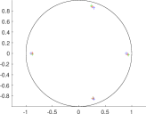
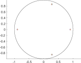
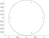
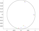
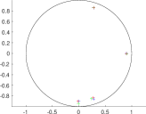
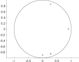
Figure 1. Rational approximation. $G(s,x)=\frac{1}{s-x}$. $X=\mathbb{D}_{1}$. $\{s_{j}\}$ are random points outside the unit disk, each with a modulus between $1.2$ and $2.2$. $n_{s}=40$. In the three columns, $\sigma$ equals to $10^{-2}$, $10^{-3}$, and $10^{-4}$, respectively. Blue, green, and red stand for the exact solution, the result before postprocessing, and the one after postprocessing. $n_{x}=4$. Top row: the test with well-separated locations. Bottom row: the test with two nearby locations.

Figure 1 summarizes the experimental results. The three columns correspond to noise levels $\sigma$ equal to $10^{-2}$, $10^{-3}$, and $10^{-4}$. In each plot, the blue markers are the exact solution $\{x_{k}\}$, the green ones are the solution of the eigenmatrix approach before the postprocessing, and the red ones are the solution after the postprocessing.

Two tests are performed. In the first one (top row), $n_{x}=4$ and $\{x_{k}\}$ are well-separated from each other. The plots show accurate recovery of the spike locations from all $\sigma$ values. In the second one (bottom row), $n_{x}=4$ and two of the spike locations are close to each other. In this harder case, the reconstruction at $\sigma=10^{-2}$ shows a noticeable error, while the results for $\sigma=10^{-3}$ and $\sigma=10^{-4}$ are accurate. The plots also suggest that the eigenmatrix approach results in fairly accurate (green) initial guesses for the postprocessing step.

Example 2 (Spectral function approximation).

The problem setup is

• $G(s,x)=\frac{1}{s-x}$.

• $X=[-1,1]$.

• $\{s_{j}\}$ is the Matsubara grid from $-\frac{(2N-1)\pi}{\beta}i$ to $\frac{(2N-1)\pi}{\beta}i$ with $\beta=100$ and $N=128$. Hence, $n_{s}=256$.

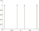
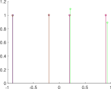
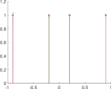
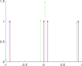
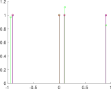
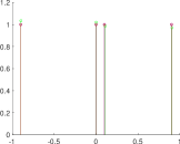
Figure 2. Spectral function approximation. $G(s,x)=\frac{1}{s-x}$. $X=[-1,1]$. $\{s_{j}\}$ is the Matsubara grid from $-\frac{(2N-1)\pi}{\beta}i$ to $\frac{(2N-1)\pi}{\beta}i$ with $\beta=100$ and $N=128$. In the three columns, $\sigma$ equals to $10^{-2}$, $10^{-3}$, and $10^{-4}$, respectively. Blue, green, and red stand for the exact solution, the result before postprocessing, and the one after postprocessing. $n_{x}=4$. Top row: the test with well-separated locations. Bottom row: the test with two nearby locations.

Figure 2 summarizes the experimental results. The three columns correspond to $\sigma$ equal to $10^{-2}$, $10^{-3}$, and $10^{-4}$, respectively. The blue, green, and red spikes denote the exact solution of the reconstructions before and after postprocessing, respectively.

Two tests are performed. In the first one (top row), $n_{x}=4$ and $\{x_{k}\}$ are well-separated. The reconstructions are accurate for all $\sigma$ values. In the second one (bottom row), $n_{x}=4$ and two of the spike locations are within $0.1$ distance from each other. In this harder case, the reconstructions remain accurate for all $\sigma$ values. Notice that the eigenmatrix provides a sufficiently accurate initial guess for postprocessing.

Example 3 (Fourier inversion).

The problem setup is

• $G(s,x)=\exp(\pi isx)$.

• $X=[-1,1]$.

• $\{s_{j}\}$ are randomly chosen points in $[-5,5]$. $n_{s}=128$.

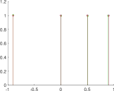
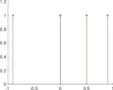
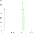
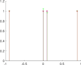
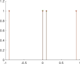
Figure 3. Fourier inversion. $G(s,x)=\exp(\pi isx)$. $X=[-1,1]$. $\{s_{j}\}$ are randomly chosen points in $[-5,5]$. $n_{s}=128$. In the three columns, $\sigma$ equals to $10^{-2}$, $10^{-3}$, and $10^{-4}$, respectively. Blue, green, and red stand for the exact solution, the result before postprocessing, and the one after postprocessing. $n_{x}=4$. Top row: the test with well-separated locations. Bottom row: the test with two nearby locations.

Figure 3 summarizes the experimental results. The three columns correspond to $\sigma$ equal to $10^{-2}$, $10^{-3}$, and $10^{-4}$. The blue, green, and red spikes denote the exact solution of the reconstructions before and after postprocessing, respectively.

Two tests are performed. In the first one (top row), $n_{x}=4$ and $\{x_{k}\}$ are well-separated. The reconstructions are accurate for all $\sigma$ values. In the second one (bottom row), $n_{x}=4$ and two of the spike locations are within $0.1$ distance from each other. The reconstructions are also accurate for all $\sigma$ values. The eigenmatrix is again able to provide sufficient accurate initial guesses for the postprocessing step.

Example 4 (Laplace inversion).

The problem setup is

• $G(s,x)=\exp(-sx)$.

• $X=[0,2]$. $x=\phi(t)=t+1$ maps from $[-1,1]$ to $X$,

• $\{s_{j}\}$ are random samples in $[0,10]$. $n_{s}=100$.

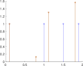
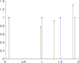
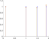
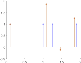
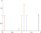
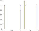
Figure 4. Laplace inversion. $G(s,x)=\exp(-sx)$. $X=[0,2]$. $\{s_{j}\}$ are random samples in $[0,10]$. $n_{s}=100$. In the three columns, $\sigma$ equals to $10^{-5}$, $10^{-6}$, and $10^{-7}$, respectively. Blue, green, and red stand for the exact solution, the result before postprocessing, and the one after postprocessing. $n_{x}=4$. Top row: the test with well-separated locations. Bottom row: the test with two nearby locations.

Figure 4 summarizes the experimental results. The inverse Laplace transform is well-known for its sensitivity to noise. As a result, significantly smaller noise magnitudes are used in this example: the three columns correspond to $\sigma$ equal to $10^{-5}$, $10^{-6}$, and $10^{-7}$. The blue, green, and red spikes still denote the exact solution of the reconstructions before and after postprocessing, respectively.

Two tests are performed. In the first one (top row), $n_{x}=4$ and $\{x_{k}\}$ are well-separated. The reconstructions are acceptable for $\sigma=10^{-6}$ and accurate for $\sigma=10^{-7}$. In the second harder test (bottom row), $n_{x}=4$ and two of the spike locations are within $0.25$ distance from each other. The reconstructions provide reasonable reconstructions at $\sigma=10^{-7}$, but significant errors for larger $\sigma$ values.

Example 5 (Sparse deconvolution).

The problem setup is

• $G(s,x)=\frac{1}{1+\gamma(s-x)^{2}}$ with $\gamma=4$.

• $X=[-1,1]$.

• $\{s_{j}\}$ are random samples from $[-5,5]$. $n_{s}=100$.

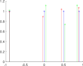
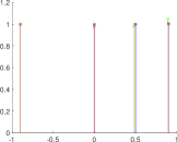
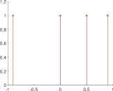
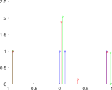
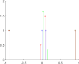
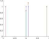
Figure 5. Sparse deconvolution. $G(s,x)=\frac{1}{1+\gamma(s-x)^{2}}$ with $\gamma=4$. $X=[-1,1]$. $\{s_{j}\}$ are random samples from $[-5,5]$. $n_{s}=100$. In the three columns, $\sigma$ equals to $10^{-2}$, $10^{-3}$, and $10^{-4}$, respectively. Blue, green, and red stand for the exact solution, the result before postprocessing, and the one after postprocessing. $n_{x}=4$. Top row: the test with well-separated locations. Bottom row: the test with two nearby locations.

Figure 5 summarizes the experimental results. The three columns correspond to $\sigma$ equal to $10^{-2}$, $10^{-3}$, and $10^{-4}$. The blue, green, and red spikes denote the exact solution of the reconstructions before and after postprocessing, respectively.

Two tests are performed. In the first one (top row), $n_{x}=4$ and $\{x_{k}\}$ are well-separated. The reconstructions are reasonable for $\sigma=10^{-2}$ and accurate for the smaller $\sigma$ values. In the second one (bottom row), $n_{x}=4$ and two of the spike locations are within $0.1$ distance from each other. The reconstructions are accurate for $\sigma$ equal to $10^{-3}$ and $10^{-4}$.

Remark 7.

The numerical experience suggests two lessons important for accurate reconstruction. First, it is important to fully exploit the prior information about the support of the spikes, i.e., making the candidate parameter set $X$ as compact as possible. Second, using the Chebyshev grid (for the real case) and the uniform grid (for the complex case) ensures that $M\mathbf{g}(x)\approx x\mathbf{g}(x)$ up to a high accuracy numerically.

5. Discussions

This paper introduces the eigenmatrix construction for unstructured sparse recovery problems. As a data-driven approach, it assumes no structure on the sample locations and offers a rather unified framework for such sparse recovery problems. There are several directions for future work.

• Providing the error estimates of the eigenmatrix approach for the problems mentioned in Section 1.

• Once the eigenmatrix is constructed, the recovery algorithm presented above follows Prony’s method and the ESPRIT algorithm. An immediate extension is to combine the eigenmatrix with other algorithms, such as MUSIC and the matrix pencil method.