Fourier Features for Identifying Differential Equations (FourierIdent)

Mengyi Tang, Hao Liu, Wenjing Liao, Sung Ha Kang School of Mathematics, Georgia Institute of Technology, Atlanta, GA 30332-0160. Email: tangmengyi@gatech.edu Department of Mathematics, Hong Kong Baptist University. Email: haoliu@ hkbu.edu.hk. Research is partially supported by HKBU 179356, NSFC 12201530 and HKRGC ECS 22302123. School of Mathematics, Georgia Institute of Technology, Atlanta, GA 30332-0160. Email: wliao60@gatech.edu. This work was partially funded by NSF 2145167.School of Mathematics, Georgia Institute of Technology, Atlanta, GA 30332-0160. Email: kang@math.gatech.edu. This work was partially funded by Simons Foundation grant 584960.
Abstract

We investigate the benefits and challenges of utilizing the frequency information in differential equation identification. Solving differential equations and Fourier analysis are closely related, yet there is limited work in exploring this connection in the identification of differential equations. Given a single realization of the differential equation perturbed by noise, we aim to identify the underlying differential equation governed by a linear combination of linear and nonlinear differential and polynomial terms in the frequency domain. This is challenging due to large magnitudes and sensitivity to noise. We introduce a Fourier feature denoising, and define the meaningful data region and the core regions of features to reduce the effect of noise in the frequency domain. We use Subspace Pursuit on the core region of the time derivative feature, and introduce a group trimming step to refine the support. We further introduce a new energy based on the core regions of features for coefficient identification. Utilizing the core regions of features serves two critical purposes: eliminating the low-response regions dominated by noise, and enhancing the accuracy in coefficient identification. The proposed method is tested on various differential equations with linear, nonlinear, and high-order derivative feature terms. Our results demonstrate the advantages of the proposed method, particularly on complex and highly corrupted datasets.

1 Introduction

Differential Equations are widely used to describe physical laws. The original discoveries of differential equations for real-world physical processes typically require a good understanding of the physical laws, and supportive evidence from empirical observations. In recent years, data-driven discoveries of differential equations become popular, where one can utilize data to identify the underlying equation.

This paper studies this inverse problem of identifying a differential equation in the form of

u(x,t)t=G(u)=l=1Lclgl(u),𝑢𝑥𝑡𝑡𝐺𝑢superscriptsubscript𝑙1𝐿subscript𝑐𝑙subscript𝑔𝑙𝑢\frac{\partial u(x,t)}{\partial t}=G(u)=\sum_{l=1}^{L}c_{l}g_{l}(u), (1)

from a single trajectory of noisy observations. Our objective is to find the unknown coefficient vector 𝒄=(cl)l=1,,LL𝒄subscriptsubscript𝑐𝑙𝑙1𝐿superscript𝐿\boldsymbol{c}=(c_{l})_{l=1,\ldots,L}\in\mathbb{R}^{L}, including the support of the vector and the value of each clsubscript𝑐𝑙c_{l} to identify the differential equation. The form of (1) includes a wide range of PDEs in science and engineering applications, such as the heat equation, transport equation, Burgers’ equation, Korteweg-de Vires (KdV) equation, Kuramoto-Sivashinsky (KS) equation, and many others. This inverse problem is often regarded as the model identification problem, where one identifies the active features in a large dictionary, which is more challenging than the parameter estimation problem when the PDE form is given.

The identification of differential equations has a long history in science and engineering, dating back to 1970s [1, 3]. From 1980s to 2000s, parameter estimation in differential equations was widely studied [2, 4, 24, 29, 12]. In recent years, sparse regression was introduced to the model identification problem, which allows one to identify a small number of active features in the underlying equation from a large dictionary, e.g., Sparse Identification of Nonlinear Dynamics (SINDy) [5, 7, 18, 26], PDE identification via data discovery and sparse optimization [28], using differential terms for the dictionary [13, 19, 26, 28, 14], and theoretical studies [15, 16]. Recent progress using weak formulation of features have significantly improved the robustness in the identification of differential equations, e.g., [8, 11, 10, 21, 22, 23, 25, 30]: A well-designed test function is introduced in [21, 22], a statistical approach with bootstrap in [7], and improvements in sparsity-promotion methods in [13, 27, 30].

In this paper, the governing function G(u)𝐺𝑢G(u) in (1) is assumed to be a linear combination of linear and nonlinear features of u𝑢u, e.g. the gl(u)subscript𝑔𝑙𝑢g_{l}(u)’s are either monomials uβsuperscript𝑢𝛽u^{\beta} or spatial derivatives of monomials αxα(uβ)superscript𝛼superscript𝑥𝛼superscript𝑢𝛽\frac{\partial^{\alpha}}{\partial x^{\alpha}}(u^{\beta}), where α,β𝛼𝛽\alpha,\beta are nonnegative integers. Motivated by the weak formulation of features in [21, 30], we consider identifying differential equation directly in the frequency domain:

{u(x,t)t}={G(u)}=l=1Lcl{gl(u)},𝑢𝑥𝑡𝑡𝐺𝑢superscriptsubscript𝑙1𝐿subscript𝑐𝑙subscript𝑔𝑙𝑢\mathcal{F}\left\{\frac{\partial u(x,t)}{\partial t}\right\}=\mathcal{F}\{G(u)\}=\sum_{l=1}^{L}c_{l}\mathcal{F}\left\{g_{l}(u)\right\}, (2)

where =x,tsubscript𝑥𝑡\mathcal{F}=\mathcal{F}_{x,t} denotes the two-dimensional Fourier transform in x𝑥x and t𝑡t.

Parameter estimation for differential equations in the frequency domain has been considered in science and engineering applications. In [32], a sample maximum likelihood estimator in the frequency domain was used to identify some spatially dependent parameters in a parabolic equation, from the given PDE form. In [9], a frequency domain identification technique was proposed to estimate Linear Parameter-Varying differential equations with weighted nonlinear least squares. [17] examined how physics-informed neural networks successively capture different frequencies of the solution such that the low-frequency components is captured at the beginning of training then the high-frequency components are captured as the training process proceeds. The authors in [33] considered cutting the given data in the frequency domain after numerical differentiation of the neural-network-denoised data in the model identification problem. The authors in [34] provided a mathematical theory on the possibility of learning a PDE from a single solution trajectory. While the frequency information of PDEs has been considered in some identification methods in the literature, there is no general framework to identify an unknown PDE using frequency responses.

We propose to use Fourier features for IDENTifying differential equations (FourierIdent) in this paper. After taking the Fourier transform of (1), we perform model selection and parameter estimation on (2) in the frequency domain, which is different from existing works on model identification in the physical domain. For example in [21, 30], the integral forms are calculated through convolution and evaluated in the frequency domain using the Fast Fourier Transform (FFT), while the rest of the computation is performed in the physical domain with the inverse FFT. We propose a robust framework, FourierIdent, for identifying differential equations directly in the frequency domain. If the coefficients are successfully identified, the resulting governing equations in the physical domain and in the frequency domain are identical.

The contributions of this paper are summarized as follows:

  1. 1.

    We propose a stable denoising method in the frequency domain to effectively handle large frequency magnitudes and to improve the robustness against noise. We use Fourier analysis and fit the correct decay of the coefficients to define the meangingful data region, and define the core regions of features for identification. The Fourier transform is computed through FFT for efficiency.

  2. 2.

    We develop FourierIdent to identify the differential equation from a single noisy trajectory of the PDE in frequency domain. Within this framework, we use the Subspace Pursuit greedy algorithm and propose group trimming to find the coefficient support at each sparsity level. We further propose a new energy based on the core regions of features to refine the coefficient identification.

  3. 3.

    FourierIdent shows benefits in identifying differential equations under high noise levels, and when the given data have a complex pattern, e.g., with rich information in different frequency modes. We present various numerical experimental results in comparison with WSINDy [21] and WeakIdent [30].

This paper is organized as follows: In Section 2, we provide the problem setup and the formulation of Fourier features. The error analysis of using one Fourier feature is discussed in Subsection 2.1. In Section 3, we propose the denoising method for Fourier features and define the core regions of features in the frequency domain. In Section 4, we present the methodology of FourerIdent, using Subspace Pursuit, group trimming and the new enegry based on the core regions of features for coefficient identification. In Section 5 and 6, we provide details of implementation and numerical results of FourierIdent. We conclude the paper with remarks in Section 7.

2 Problem set-up and Fourier features

We present FourierIdent on one-dimensional PDEs, but our proposed method can be extended to high-dimensional PDEs. We let the physical domain be Ω=[0,X]×[0,T]Ω0𝑋0𝑇\Omega=[0,X]\times[0,T] with X>0,T>0formulae-sequence𝑋0𝑇0X>0,T>0, and data to be sampled on a uniform grid with step size ΔxΔ𝑥\Delta x, and ΔtΔ𝑡\Delta t. We denote xi=iΔx,tn=nΔtformulae-sequencesubscript𝑥𝑖𝑖Δ𝑥superscript𝑡𝑛𝑛Δ𝑡x_{i}=i\Delta x,t^{n}=n\Delta t, and the PDE solution at (xi,tn)subscript𝑥𝑖superscript𝑡𝑛(x_{i},t^{n}) as Uin=u(xi,tn)superscriptsubscript𝑈𝑖𝑛𝑢subscript𝑥𝑖superscript𝑡𝑛U_{i}^{n}=u(x_{i},t^{n}). Our observation of the solution at (xi,tn)subscript𝑥𝑖superscript𝑡𝑛(x_{i},t^{n}) is contaminated by noise such that

Unoise,in=Uin+ϵinfor(xi,tn)Ω,superscriptsubscript𝑈𝑛𝑜𝑖𝑠𝑒𝑖𝑛superscriptsubscript𝑈𝑖𝑛superscriptsubscriptitalic-ϵ𝑖𝑛forsubscript𝑥𝑖superscript𝑡𝑛ΩU_{noise,i}^{n}=U_{i}^{n}+\epsilon_{i}^{n}\;\;{\rm for}\;\;(x_{i},t^{n})\in\Omega, (3)

where ϵinsuperscriptsubscriptitalic-ϵ𝑖𝑛\epsilon_{i}^{n} represents zero-mean noise at each point (xi,tn)subscript𝑥𝑖superscript𝑡𝑛(x_{i},t^{n}). We denote the given data as

𝒟={Unoise,in|i=0,1,2,,x1,n=0,1,,t1}x×t,𝒟conditional-setsuperscriptsubscript𝑈𝑛𝑜𝑖𝑠𝑒𝑖𝑛formulae-sequence𝑖012subscript𝑥1𝑛01subscript𝑡1superscriptsubscript𝑥subscript𝑡\mathcal{D}=\{U_{noise,i}^{n}|i=0,1,2,...,\mathbb{N}_{x}-1,n=0,1,...,\mathbb{N}_{t}-1\}\in\mathbb{R}^{\mathbb{N}_{x}\times\mathbb{N}_{t}}, (4)

where xsubscript𝑥\mathbb{N}_{x} and tsubscript𝑡\mathbb{N}_{t}\in\mathbb{N} are the discretization sizes in the spatial and temporal dimensions. We assume that the underlying equation has the form of (1):

ut(x,t)=l=1Lclgl=l=1Lclαlfl(u)xαl,withfl(u)=uβl,formulae-sequence𝑢𝑡𝑥𝑡superscriptsubscript𝑙1𝐿subscript𝑐𝑙subscript𝑔𝑙superscriptsubscript𝑙1𝐿subscript𝑐𝑙superscriptsubscript𝛼𝑙subscript𝑓𝑙𝑢superscript𝑥subscript𝛼𝑙withsubscript𝑓𝑙𝑢superscript𝑢subscript𝛽𝑙\displaystyle\frac{\partial u}{\partial t}(x,t)=\sum_{l=1}^{L}c_{l}g_{l}=\sum_{l=1}^{L}c_{l}\frac{\partial^{\alpha_{l}}f_{l}(u)}{\partial x^{\alpha_{l}}},\ \text{with}\ f_{l}(u)=u^{\beta_{l}}, (5)

where L𝐿L is the total number of features in the dictionary which consists of feature terms as {αlfl(u)xαl}l=1Lsuperscriptsubscriptsuperscriptsubscript𝛼𝑙subscript𝑓𝑙𝑢superscript𝑥subscript𝛼𝑙𝑙1𝐿\left\{\frac{\partial^{\alpha_{l}}f_{l}(u)}{\partial x^{\alpha_{l}}}\right\}_{l=1}^{L}. We use the index l𝑙l and (αl,βl)subscript𝛼𝑙subscript𝛽𝑙(\alpha_{l},\beta_{l}) to indicate that the l𝑙l-th feature glsubscript𝑔𝑙g_{l} which is αluβlxαlsuperscriptsubscript𝛼𝑙superscript𝑢subscript𝛽𝑙superscript𝑥subscript𝛼𝑙\frac{\partial^{\alpha_{l}}u^{\beta_{l}}}{\partial x^{\alpha_{l}}}, the αlsubscript𝛼𝑙\alpha_{l}-order derivative of the monomial uβlsuperscript𝑢subscript𝛽𝑙u^{\beta_{l}} where αl,βlsubscript𝛼𝑙subscript𝛽𝑙\alpha_{l},\beta_{l} are nonnegative integers.

Since we consider PDEs in the frequency domain, we assume that u𝑢u is a periodic function in x𝑥x and t𝑡t. For non-periodic functions, we extend the function to a periodic function, which is to be discussed in Subsection 5.1. We define the Fourier transform of u(x,t)𝑢𝑥𝑡u(x,t) as:

(u)[ξx,ξt]=0T0Xu(x,t)e(ξxxX+ξttT)2π1𝑑x𝑑t.𝑢subscript𝜉𝑥subscript𝜉𝑡superscriptsubscript0𝑇superscriptsubscript0𝑋𝑢𝑥𝑡superscript𝑒subscript𝜉𝑥𝑥𝑋subscript𝜉𝑡𝑡𝑇2𝜋1differential-d𝑥differential-d𝑡\mathcal{F}(u)[\xi_{x},\xi_{t}]=\int_{0}^{T}\int_{0}^{X}u(x,t)e^{-(\frac{\xi_{x}{x}}{X}+\frac{\xi_{t}{t}}{T})2\pi\sqrt{-1}}dxdt.

The Fourier transform of (5) with respect to x𝑥x and t𝑡t becomes

2πTξt1(u)[ξx,ξt]2𝜋𝑇subscript𝜉𝑡1𝑢subscript𝜉𝑥subscript𝜉𝑡\displaystyle\frac{2\pi}{T}\xi_{t}\sqrt{-1}\mathcal{F}(u)[\xi_{x},\xi_{t}]
=\displaystyle= l=1Lcl(2πXξx1)αl(fl)[ξx,ξt]superscriptsubscript𝑙1𝐿subscript𝑐𝑙superscript2𝜋𝑋subscript𝜉𝑥1subscript𝛼𝑙subscript𝑓𝑙subscript𝜉𝑥subscript𝜉𝑡\displaystyle\sum_{l=1}^{L}c_{l}\left(\frac{2\pi}{X}\xi_{x}\sqrt{-1}\right)^{\alpha_{l}}\mathcal{F}(f_{l})[\xi_{x},\xi_{t}]
=\displaystyle= [(2πXξx1)α1(f1(u))(2πXξx1)αl(f2(u))(2πXξx1)αL(fL(u))]𝐜.matrixsuperscript2𝜋𝑋subscript𝜉𝑥1subscript𝛼1subscript𝑓1𝑢superscript2𝜋𝑋subscript𝜉𝑥1subscript𝛼𝑙subscript𝑓2𝑢superscript2𝜋𝑋subscript𝜉𝑥1subscript𝛼𝐿subscript𝑓𝐿𝑢𝐜\displaystyle\begin{bmatrix}(\frac{2\pi}{X}\xi_{x}\sqrt{-1})^{\alpha_{1}}\mathcal{F}(f_{1}(u))&\cdots&(\frac{2\pi}{X}\xi_{x}\sqrt{-1})^{\alpha_{l}}\mathcal{F}(f_{2}(u))&\cdots&(\frac{2\pi}{X}\xi_{x}\sqrt{-1})^{\alpha_{L}}\mathcal{F}(f_{L}(u))\end{bmatrix}\mathbf{c}. (6)

The first term in (6) is the Fourier feature of utsubscript𝑢𝑡u_{t}, and (2πXξx1)αl(fl(u))superscript2𝜋𝑋subscript𝜉𝑥1subscript𝛼𝑙subscript𝑓𝑙𝑢(\frac{2\pi}{X}\xi_{x}\sqrt{-1})^{\alpha_{l}}\mathcal{F}(f_{l}(u)) in the right of (6) is that of the l𝑙l-th feature in the library, i.e., αluβlxαlsuperscriptsubscript𝛼𝑙superscript𝑢subscript𝛽𝑙superscript𝑥subscript𝛼𝑙\frac{\partial^{\alpha_{l}}u^{\beta_{l}}}{\partial x^{\alpha_{l}}}.

Our idea is to find the support and values of the coefficient vector 𝐜𝐜\mathbf{c} at the frequency modes (ξx,ξt)subscript𝜉𝑥subscript𝜉𝑡(\xi_{x},\xi_{t}) for ξx=0,1,,x1,ξt=0,1,2,t1formulae-sequencesubscript𝜉𝑥01subscript𝑥1subscript𝜉𝑡012subscript𝑡1\xi_{x}=0,1,...,\mathbb{N}_{x}-1,\xi_{t}=0,1,2...,\mathbb{N}_{t}-1. We denote h=(ξx,ξt)subscript𝜉𝑥subscript𝜉𝑡h=\mathcal{H}(\xi_{x},\xi_{t}) as the index of the frequency mode (ξx,ξt)subscript𝜉𝑥subscript𝜉𝑡(\xi_{x},\xi_{t}), where \mathcal{H} is a map from the frequency mode (ξx,ξt)subscript𝜉𝑥subscript𝜉𝑡(\xi_{x},\xi_{t}) to the unique index h{1,2,,H}12𝐻h\in\{1,2,\ldots,H\} with H=#{(ξx,ξt):ξx=0,1,,x1,ξt=0,1,,t1}=xt𝐻#conditional-setsubscript𝜉𝑥subscript𝜉𝑡formulae-sequencesubscript𝜉𝑥01subscript𝑥1subscript𝜉𝑡01subscript𝑡1subscript𝑥subscript𝑡H=\#\{(\xi_{x},\xi_{t}):\xi_{x}=0,1,...,\mathbb{N}_{x}-1,\xi_{t}=0,1,...,\mathbb{N}_{t}-1\}=\mathbb{N}_{x}\mathbb{N}_{t}. The notation ##\# denotes the cardinality of a set. FourierIdent aims to solve a discrete Fourier system of (6)

𝑭𝒄=𝒃,𝑭𝒄𝒃\boldsymbol{F}\boldsymbol{c}=\boldsymbol{b}, (7)

where

𝑭=(ah,l)H×L,𝒄=(cl)L,𝒃=(bh)H,formulae-sequence𝑭subscript𝑎𝑙superscript𝐻𝐿𝒄subscript𝑐𝑙superscript𝐿𝒃subscript𝑏superscript𝐻\boldsymbol{F}=(a_{h,l})\in\mathbb{C}^{H\times L},\;\;\boldsymbol{c}=(c_{l})\in\mathbb{R}^{L},\;\;\boldsymbol{b}=(b_{h})\in\mathbb{C}^{H},

for

ah,l=(2πξxX1)αlp=0x1q=0t1{e(2πpxξx+2πqtξt)1(Unoise,pq)βl}ΔxΔtsubscript𝑎𝑙superscript2𝜋subscript𝜉𝑥𝑋1subscript𝛼𝑙superscriptsubscript𝑝0subscript𝑥1superscriptsubscript𝑞0subscript𝑡1superscript𝑒2𝜋𝑝subscript𝑥subscript𝜉𝑥2𝜋𝑞subscript𝑡subscript𝜉𝑡1superscriptsuperscriptsubscript𝑈𝑛𝑜𝑖𝑠𝑒𝑝𝑞subscript𝛽𝑙Δ𝑥Δ𝑡a_{h,l}=\left(\frac{2\pi\xi_{x}}{X}\sqrt{-1}\right)^{\alpha_{l}}\sum_{p=0}^{\mathbb{N}_{x}-1}\sum_{q=0}^{\mathbb{N}_{t}-1}\Biggl{\{}e^{\displaystyle-\left(\frac{2\pi p}{\mathbb{N}_{x}}\xi_{x}+\frac{2\pi q}{\mathbb{N}_{t}}\xi_{t}\right)\sqrt{-1}}\left(U_{noise,p}^{q}\right)^{\beta_{l}}\Biggr{\}}\Delta x\Delta t

and

bh,l=(2πξtT1)p=0x1q=0t1{e(2πpxξx+2πqtξt)1Unoise,pq}ΔxΔt.subscript𝑏𝑙2𝜋subscript𝜉𝑡𝑇1superscriptsubscript𝑝0subscript𝑥1superscriptsubscript𝑞0subscript𝑡1superscript𝑒2𝜋𝑝subscript𝑥subscript𝜉𝑥2𝜋𝑞subscript𝑡subscript𝜉𝑡1superscriptsubscript𝑈𝑛𝑜𝑖𝑠𝑒𝑝𝑞Δ𝑥Δ𝑡b_{h,l}=\left(\frac{2\pi\xi_{t}}{T}\sqrt{-1}\right)\sum_{p=0}^{\mathbb{N}_{x}-1}\sum_{q=0}^{\mathbb{N}_{t}-1}\Biggl{\{}e^{\displaystyle-\left(\frac{2\pi p}{\mathbb{N}_{x}}\xi_{x}+\frac{2\pi q}{\mathbb{N}_{t}}\xi_{t}\right)\sqrt{-1}}U_{noise,p}^{q}\Biggr{\}}\Delta x\Delta t.

Here Δx=Xx,Δt=Ttformulae-sequenceΔ𝑥𝑋subscript𝑥Δ𝑡𝑇subscript𝑡\Delta x=\frac{X}{\mathbb{N}_{x}},\Delta t=\frac{T}{\mathbb{N}_{t}}. The l𝑙l-th column of 𝑭𝑭\boldsymbol{F} is the discrete Fourier feature associated with the l𝑙l-th feature in the dictionary, and the vector 𝒃𝒃\boldsymbol{b} contains the discrete Fourier feature for utsubscript𝑢𝑡u_{t}. The objective of this paper is to find the support and values of this coefficient vector in (7)

𝒄=[c1,c2,,cL]𝒄superscriptsubscript𝑐1subscript𝑐2subscript𝑐𝐿top\boldsymbol{c}=[c_{1},c_{2},\cdots,c_{L}]^{\top}

from the given data 𝒟𝒟\mathcal{D}.

2.1 Error analysis for Fourier features

We analyze the error of the linear system (7) with discrete Fourier features. Assume that {ϵin}superscriptsubscriptitalic-ϵ𝑖𝑛\{\epsilon_{i}^{n}\} in (3) are i.i.d and have zero-mean such that 𝔼[ϵin]=0𝔼delimited-[]superscriptsubscriptitalic-ϵ𝑖𝑛0\mathbb{E}[\epsilon_{i}^{n}]=0. Denote the true coefficient vector for the underlying PDE by 𝒄𝒄\boldsymbol{c}, and the support of the true coefficient vector by Supp={l:cl0}superscriptSuppconditional-set𝑙subscript𝑐𝑙0{\rm Supp}^{*}=\{l:\ c_{l}\neq 0\}. The true coefficients satisfy the following equation :

2πTξt1(u)[ξx,ξt]=lSuppcl(2πXξx1)αl(fl)[ξx,ξt],2𝜋𝑇subscript𝜉𝑡1𝑢subscript𝜉𝑥subscript𝜉𝑡subscript𝑙superscriptSuppsubscript𝑐𝑙superscript2𝜋𝑋subscript𝜉𝑥1subscript𝛼𝑙subscript𝑓𝑙subscript𝜉𝑥subscript𝜉𝑡\frac{2\pi}{T}\xi_{t}\sqrt{-1}\mathcal{F}(u)[\xi_{x},\xi_{t}]=\sum_{l\in\rm{Supp}^{*}}c_{l}\left(\frac{2\pi}{X}\xi_{x}\sqrt{-1}\right)^{\alpha_{l}}\mathcal{F}(f_{l})[\xi_{x},\xi_{t}], (8)

for ξx=0,1,,x1,ξt=0,1,,t1formulae-sequencesubscript𝜉𝑥01subscript𝑥1subscript𝜉𝑡01subscript𝑡1\xi_{x}=0,1,...,\mathbb{N}_{x}-1,\xi_{t}=0,1,...,\mathbb{N}_{t}-1.

The Lsubscript𝐿L_{\infty}-residual of (7) consists of two errors: one is the discretization error of Fourier features and the other is the error from noise:

e=𝑭𝒄𝒃eFourier+enoise.𝑒subscriptnorm𝑭𝒄𝒃subscript𝑒Fouriersubscript𝑒noisee=\|\boldsymbol{F}\boldsymbol{c}-\boldsymbol{b}\|_{\infty}\leq{e}_{\rm{Fourier}}+{e}_{\rm{noise}}.

The discretization error of Fourier features is

eFourier=subscript𝑒Fourierabsent\displaystyle{e}_{\rm{Fourier}}= maxξx,ξt|lSuppcl(2πξxX1)αlp=0x1q=0t1{e(2πpxξx+2πqtξt)1(Upq)βl}conditionalsubscriptsubscript𝜉𝑥subscript𝜉𝑡subscript𝑙superscriptSuppsubscript𝑐𝑙superscript2𝜋subscript𝜉𝑥𝑋1subscript𝛼𝑙superscriptsubscript𝑝0subscript𝑥1superscriptsubscript𝑞0subscript𝑡1superscript𝑒2𝜋𝑝subscript𝑥subscript𝜉𝑥2𝜋𝑞subscript𝑡subscript𝜉𝑡1superscriptsuperscriptsubscript𝑈𝑝𝑞subscript𝛽𝑙\displaystyle\max_{\xi_{x},\xi_{t}}\Bigg{|}\sum_{l\in\rm{Supp}^{*}}c_{l}\left(\frac{2\pi\xi_{x}}{X}\sqrt{-1}\right)^{\alpha_{l}}\sum_{p=0}^{\mathbb{N}_{x}-1}\sum_{q=0}^{\mathbb{N}_{t}-1}\Biggl{\{}e^{-\left(\frac{2\pi p}{\mathbb{N}_{x}}\xi_{x}+\frac{2\pi q}{\mathbb{N}_{t}}\xi_{t}\right)\sqrt{-1}}\left(U_{p}^{q}\right)^{\beta_{l}}\Biggr{\}}
(2πξtT1)p=0x1q=0t1{e(2πpxξx+2πqtξt)1Upq}|XTxt,conditional2𝜋subscript𝜉𝑡𝑇1superscriptsubscript𝑝0subscript𝑥1superscriptsubscript𝑞0subscript𝑡1superscript𝑒2𝜋𝑝subscript𝑥subscript𝜉𝑥2𝜋𝑞subscript𝑡subscript𝜉𝑡1superscriptsubscript𝑈𝑝𝑞𝑋𝑇subscript𝑥subscript𝑡\displaystyle-\left(\frac{2\pi\xi_{t}}{T}\sqrt{-1}\right)\sum_{p=0}^{\mathbb{N}_{x}-1}\sum_{q=0}^{\mathbb{N}_{t}-1}\Biggl{\{}e^{-\left(\frac{2\pi p}{\mathbb{N}_{x}}\xi_{x}+\frac{2\pi q}{\mathbb{N}_{t}}\xi_{t}\right)\sqrt{-1}}U_{p}^{q}\Biggr{\}}\Bigg{|}\frac{XT}{\mathbb{N}_{x}\mathbb{N}_{t}},

and decreases to 00 as the data sampling grid is refined:

limΔx,Δt0eFourier=maxξx,ξt|lSuppcl(2πXξx1)αl(uβl)[ξx,ξt]2πTξt1(u)[ξx,ξt]|=0.subscriptΔ𝑥Δ𝑡0subscript𝑒Fouriersubscriptsubscript𝜉𝑥subscript𝜉𝑡subscript𝑙superscriptSuppsubscript𝑐𝑙superscript2𝜋𝑋subscript𝜉𝑥1subscript𝛼𝑙superscript𝑢subscript𝛽𝑙subscript𝜉𝑥subscript𝜉𝑡2𝜋𝑇subscript𝜉𝑡1𝑢subscript𝜉𝑥subscript𝜉𝑡0\lim_{\Delta x,\Delta t\rightarrow 0}{e}_{\rm{Fourier}}=\max_{\xi_{x},\xi_{t}}\left|\sum_{l\in{\rm Supp}^{*}}c_{l}\left(\frac{2\pi}{X}\xi_{x}\sqrt{-1}\right)^{\alpha_{l}}\mathcal{F}(u^{\beta_{l}})[\xi_{x},\xi_{t}]-\frac{2\pi}{T}\xi_{t}\sqrt{-1}\mathcal{F}(u)[\xi_{x},\xi_{t}]\right|=0.

The error from the noise is

enoise=subscript𝑒noiseabsent\displaystyle{e}_{\rm{noise}}= maxξx,ξt|enoise[ξx,ξt]|subscriptsubscript𝜉𝑥subscript𝜉𝑡subscript𝑒noisesubscript𝜉𝑥subscript𝜉𝑡\displaystyle\max_{\xi_{x},\xi_{t}}|e_{\rm{noise}}[\xi_{x},\xi_{t}]|
=\displaystyle= maxξx,ξt|lSuppcl(2πξxX1)αlp=0x1q=0t1{e(2πpxξx+2πqtξt)1((Unoise,pq)βl(Upq)βl)}conditionalsubscriptsubscript𝜉𝑥subscript𝜉𝑡subscript𝑙superscriptSuppsubscript𝑐𝑙superscript2𝜋subscript𝜉𝑥𝑋1subscript𝛼𝑙superscriptsubscript𝑝0subscript𝑥1superscriptsubscript𝑞0subscript𝑡1superscript𝑒2𝜋𝑝subscript𝑥subscript𝜉𝑥2𝜋𝑞subscript𝑡subscript𝜉𝑡1superscriptsuperscriptsubscript𝑈𝑛𝑜𝑖𝑠𝑒𝑝𝑞subscript𝛽𝑙superscriptsuperscriptsubscript𝑈𝑝𝑞subscript𝛽𝑙\displaystyle\max_{\xi_{x},\xi_{t}}\Bigg{|}\sum_{l\in\rm{Supp}^{*}}c_{l}\left(\frac{2\pi\xi_{x}}{X}\sqrt{-1}\right)^{\alpha_{l}}\sum_{p=0}^{\mathbb{N}_{x}-1}\sum_{q=0}^{\mathbb{N}_{t}-1}\Biggl{\{}e^{-\left(\frac{2\pi p}{\mathbb{N}_{x}}\xi_{x}+\frac{2\pi q}{\mathbb{N}_{t}}\xi_{t}\right)\sqrt{-1}}\left(\left(U_{noise,p}^{q}\right)^{\beta_{l}}-\left(U_{p}^{q}\right)^{\beta_{l}}\right)\Biggr{\}}
(2πξtT1)p=0x1q=0t1{e(2πpxξx+2πqtξt)1ϵpq}|XTxt,conditional2𝜋subscript𝜉𝑡𝑇1superscriptsubscript𝑝0subscript𝑥1superscriptsubscript𝑞0subscript𝑡1superscript𝑒2𝜋𝑝subscript𝑥subscript𝜉𝑥2𝜋𝑞subscript𝑡subscript𝜉𝑡1superscriptsubscriptitalic-ϵ𝑝𝑞𝑋𝑇subscript𝑥subscript𝑡\displaystyle-\left(\frac{2\pi\xi_{t}}{T}\sqrt{-1}\right)\sum_{p=0}^{\mathbb{N}_{x}-1}\sum_{q=0}^{\mathbb{N}_{t}-1}\Biggl{\{}e^{-\left(\frac{2\pi p}{\mathbb{N}_{x}}\xi_{x}+\frac{2\pi q}{\mathbb{N}_{t}}\xi_{t}\right)\sqrt{-1}}\epsilon_{p}^{q}\Biggr{\}}\Bigg{|}\frac{XT}{\mathbb{N}_{x}\mathbb{N}_{t}}, (9)

where enoise[ξx,ξt]subscript𝑒noisesubscript𝜉𝑥subscript𝜉𝑡{e}_{\rm{noise}}[\xi_{x},\xi_{t}] denotes the residual at the frequency mode (ξx,ξt)subscript𝜉𝑥subscript𝜉𝑡(\xi_{x},\xi_{t}). In the following, we prove an upper bound for the error enoisesubscript𝑒noise{e}_{\rm noise} resulted from noise.

Theorem 1.

Consider the differential equation in (5) whose Fourier form is (8). Assume that the given data 𝒟𝒟\mathcal{D} in (4) are contaminated by i.i.d. noise: {ϵin}superscriptsubscriptitalic-ϵ𝑖𝑛\{\epsilon_{i}^{n}\} are i.i.d bounded random variables with 𝔼[ϵin]=0𝔼delimited-[]superscriptsubscriptitalic-ϵ𝑖𝑛0\mathbb{E}[\epsilon_{i}^{n}]=0 and |ϵin|ϵsuperscriptsubscriptitalic-ϵ𝑖𝑛italic-ϵ|\epsilon_{i}^{n}|\leq\epsilon for some ϵ>0italic-ϵ0\epsilon>0. The area of ΩΩ\Omega is denoted by |Ω|=XTΩ𝑋𝑇|\Omega|=XT. Then the error enoisesubscript𝑒noise{e}_{\rm noise} satisfies

enoiseXTxtSϵ+𝒪(ϵ2),subscript𝑒noise𝑋𝑇subscript𝑥subscript𝑡𝑆italic-ϵ𝒪superscriptitalic-ϵ2{e}_{\rm{noise}}\leq\frac{XT}{\mathbb{N}_{x}\mathbb{N}_{t}}S\epsilon+\mathcal{O}(\epsilon^{2}), (10)

where

S=maxξx,ξt|p=0x1q=0t1e(2πpxξx+2πqtξt)1(lSuppcl(2πξxX1)αlβl(Upq)βl12πξtT1)|.𝑆subscriptsubscript𝜉𝑥subscript𝜉𝑡superscriptsubscript𝑝0subscript𝑥1superscriptsubscript𝑞0subscript𝑡1superscript𝑒2𝜋𝑝subscript𝑥subscript𝜉𝑥2𝜋𝑞subscript𝑡subscript𝜉𝑡1subscript𝑙superscriptSuppsubscript𝑐𝑙superscript2𝜋subscript𝜉𝑥𝑋1subscript𝛼𝑙subscript𝛽𝑙superscriptsuperscriptsubscript𝑈𝑝𝑞subscript𝛽𝑙12𝜋subscript𝜉𝑡𝑇1S=\max_{\xi_{x},\xi_{t}}\Bigg{|}\sum_{p=0}^{\mathbb{N}_{x}-1}\sum_{q=0}^{\mathbb{N}_{t}-1}e^{-\left(\frac{2\pi p}{\mathbb{N}_{x}}\xi_{x}+\frac{2\pi q}{\mathbb{N}_{t}}\xi_{t}\right)\sqrt{-1}}\left(\sum_{l\in\rm{Supp}^{*}}c_{l}\left(\frac{2\pi\xi_{x}}{X}\sqrt{-1}\right)^{\alpha_{l}}\beta_{l}(U_{p}^{q})^{\beta_{l}-1}-\frac{2\pi\xi_{t}}{T}\sqrt{-1}\right)\Bigg{|}. (11)
Proof.

Following the definition of enoisesubscript𝑒noise{e}_{\rm{noise}} in (9), we have

enoise=subscript𝑒noiseabsent\displaystyle{e}_{\rm{noise}}= maxξx,ξt|lSuppcl(2πξxX1)αlp=0x1q=0t1{e(2πpxξx+2πqtξt)1(βl(Upq)βl1ϵpq+𝒪((ϵpq)2))}conditionalsubscriptsubscript𝜉𝑥subscript𝜉𝑡subscript𝑙superscriptSuppsubscript𝑐𝑙superscript2𝜋subscript𝜉𝑥𝑋1subscript𝛼𝑙superscriptsubscript𝑝0subscript𝑥1superscriptsubscript𝑞0subscript𝑡1superscript𝑒2𝜋𝑝subscript𝑥subscript𝜉𝑥2𝜋𝑞subscript𝑡subscript𝜉𝑡1subscript𝛽𝑙superscriptsuperscriptsubscript𝑈𝑝𝑞subscript𝛽𝑙1superscriptsubscriptitalic-ϵ𝑝𝑞𝒪superscriptsuperscriptsubscriptitalic-ϵ𝑝𝑞2\displaystyle\max_{\xi_{x},\xi_{t}}\Bigg{|}\sum_{l\in\rm{Supp}^{*}}c_{l}\left(\frac{2\pi\xi_{x}}{X}\sqrt{-1}\right)^{\alpha_{l}}\sum_{p=0}^{\mathbb{N}_{x}-1}\sum_{q=0}^{\mathbb{N}_{t}-1}\Biggl{\{}e^{-\left(\frac{2\pi p}{\mathbb{N}_{x}}\xi_{x}+\frac{2\pi q}{\mathbb{N}_{t}}\xi_{t}\right)\sqrt{-1}}\left(\beta_{l}\left(U_{p}^{q}\right)^{\beta_{l}-1}\epsilon_{p}^{q}+\mathcal{O}((\epsilon_{p}^{q})^{2})\right)\Biggr{\}}
(2πξtT1)p=0x1q=0t1{e(2πpxξx+2πqtξt)1ϵpq}|XTxtXTxtSϵ+𝒪(ϵ2),conditional2𝜋subscript𝜉𝑡𝑇1superscriptsubscript𝑝0subscript𝑥1superscriptsubscript𝑞0subscript𝑡1superscript𝑒2𝜋𝑝subscript𝑥subscript𝜉𝑥2𝜋𝑞subscript𝑡subscript𝜉𝑡1superscriptsubscriptitalic-ϵ𝑝𝑞𝑋𝑇subscript𝑥subscript𝑡𝑋𝑇subscript𝑥subscript𝑡𝑆italic-ϵ𝒪superscriptitalic-ϵ2\displaystyle-\left(\frac{2\pi\xi_{t}}{T}\sqrt{-1}\right)\sum_{p=0}^{\mathbb{N}_{x}-1}\sum_{q=0}^{\mathbb{N}_{t}-1}\Biggl{\{}e^{-\left(\frac{2\pi p}{\mathbb{N}_{x}}\xi_{x}+\frac{2\pi q}{\mathbb{N}_{t}}\xi_{t}\right)\sqrt{-1}}\epsilon_{p}^{q}\Biggr{\}}\Bigg{|}\frac{XT}{\mathbb{N}_{x}\mathbb{N}_{t}}\leq\frac{XT}{\mathbb{N}_{x}\mathbb{N}_{t}}S\epsilon+\mathcal{O}(\epsilon^{2}),

where S𝑆S is defined in (11). ∎

First, Theorem 1 shows that the error 𝒆noisesubscript𝒆noise\boldsymbol{e}_{\rm{noise}} scales linearly with respect to the noise level ϵitalic-ϵ\epsilon. In comparison, numerical differentiation of the features in the physical domain can give error as

𝒪(Δt+Δxp+1r+ϵΔt+ϵ(Δx)r)𝒪Δ𝑡Δsuperscript𝑥𝑝1𝑟italic-ϵΔ𝑡italic-ϵsuperscriptΔ𝑥𝑟\mathcal{O}\left(\Delta t+\Delta x^{p+1-r}+\frac{\epsilon}{\Delta t}+\frac{\epsilon}{(\Delta x)^{r}}\right)

where r𝑟r is the highest order of derivatives for the active features in the true support, and numerical differentiation is carried by interpolating the data by a p𝑝pth order polynomial [19, 13]. The noise is magnified by 1/Δt1Δ𝑡1/\Delta t and 1/(Δx)r1superscriptΔ𝑥𝑟1/(\Delta x)^{r}, which shows the challenges of dealing with noisy data. Theorem 1 shows the formulation of Fourier features (10) is more robust against noise in comparison with numerical formulation of differential features. In the weak formulation, such as WeakIdent[30], the error (resulted from noise) of the linear system also scales linearly with respect to noise,

enoiseweaksuperscriptsubscript𝑒noiseweak\displaystyle{e}_{\rm noise}^{\rm weak} S¯|Ωh|ϵ+𝒪(ϵ2),absentsuperscript¯𝑆subscriptΩitalic-ϵ𝒪superscriptitalic-ϵ2\displaystyle\leq\bar{S}^{*}|\Omega_{h}|\epsilon+\mathcal{O}\left(\epsilon^{2}\right), (12)
withS¯=maxhsup(xj,tk)Ωh|lSupp(1)αlclβl(Ujk)βl1αlϕxαl(xj,tk)ϕt(xj,tk)|,withsuperscript¯𝑆subscriptsubscriptsupremumsubscript𝑥𝑗superscript𝑡𝑘subscriptΩsubscript𝑙superscriptSuppsuperscript1subscript𝛼𝑙subscript𝑐𝑙subscript𝛽𝑙superscriptsuperscriptsubscript𝑈𝑗𝑘subscript𝛽𝑙1superscriptsubscript𝛼𝑙italic-ϕsuperscript𝑥subscript𝛼𝑙subscript𝑥𝑗superscript𝑡𝑘italic-ϕ𝑡subscript𝑥𝑗superscript𝑡𝑘\displaystyle\text{with}\ \bar{S}^{*}=\max_{h}\sup_{(x_{j},t^{k})\in\Omega_{h}}\bigg{|}\sum_{l\in\rm{Supp}^{*}}(-1)^{\alpha_{l}}{c_{l}}{\beta_{l}}(U_{j}^{k})^{\beta_{l}-1}\frac{\partial^{\alpha_{l}}\phi}{\partial x^{\alpha_{l}}}(x_{j},t^{k})-\frac{\displaystyle\partial\phi}{\displaystyle\partial t}(x_{j},t^{k})\bigg{|},

where hh is an index of the test function, ΩhsubscriptΩ\Omega_{h} is the support of the hh-th test function, and |Ωh|subscriptΩ|\Omega_{h}| is the area of ΩhsubscriptΩ\Omega_{h} [30, Theorem 1]. The error bounds in both (10) and (12) scale linearly with respect to the noise level ϵitalic-ϵ\epsilon, which demonstrates that the numerical formulations of weak features and Fourier features are both robust to noise.

Secondly, the major difference between (10) and (12) is that, the error in WeakIdent is local depending on the local support ΩhsubscriptΩ\Omega_{h} of the hh-th test function, while the error in FourierIdent is global.

3 Fourier feature denoising and core regions of features

One of the main difficulties of FourierIdent is that frequency responses may have large magnitude, which is different from the linear system generated in the physical domain. As in [19, 13, 30], even in physical domain denoising is very important for coefficient identification. In this section, we propose a denoising process for FourierIdent using (i) Fourier feature denoising as in the physical domain, and defining partitions of frequency domain via (ii) the meaningful data region, and (iii) the core regions of features in the frequency domain. We give details of denoising, then present the main algorithm of FourierIdent in Section 4.

3.1 Denoising Fourier features

We first denoise Fourier features by applying convolution with a Gaussian-shape kernel ϕ(x,t)italic-ϕ𝑥𝑡\phi(x,t). By the convolution theorem, we conduct all computations of convolution in the frequency domain. This can be also applied in a restricted domain. For example, let ΛΛ\Lambda be a smaller region in the frequency domain, and the matrix 𝑭Λsubscript𝑭Λ\boldsymbol{F}_{\Lambda} and the vector 𝒃Λsubscript𝒃Λ\boldsymbol{b}_{\Lambda} be restricted to the entries from the region ΛΛ\Lambda. We let (ξx,ξt)Λsubscript𝜉𝑥subscript𝜉𝑡Λ(\xi_{x},\xi_{t})\in\Lambda, and hh be the associated index such that h=(ξx,ξt)subscript𝜉𝑥subscript𝜉𝑡h=\mathcal{H}(\xi_{x},\xi_{t}), which is also the row index of the frequency mode (ξx,ξt)subscript𝜉𝑥subscript𝜉𝑡(\xi_{x},\xi_{t}) in 𝒮(𝑭)𝒮𝑭\mathcal{S}(\boldsymbol{F}). We define the smoothing operator 𝒮𝒮\mathcal{S} on the matrix 𝑭Λsubscript𝑭Λ\boldsymbol{F}_{\Lambda} as follows:

[𝒮(𝑭)Λ]h,lsubscriptdelimited-[]𝒮subscript𝑭Λ𝑙\displaystyle[\mathcal{S}({\boldsymbol{F}})_{\Lambda}]_{h,l} (13)
=\displaystyle= (2πξx1X)αl(p=0x1q=0t1e(2πpxξx+2πqtξt)1(Unoise,pq)βl)(p=0x1q=0t1e(2πpxξx+2πqtξt)1Φpq),superscript2𝜋subscript𝜉𝑥1𝑋subscript𝛼𝑙superscriptsubscript𝑝0subscript𝑥1superscriptsubscript𝑞0subscript𝑡1superscript𝑒2𝜋𝑝subscript𝑥subscript𝜉𝑥2𝜋𝑞subscript𝑡subscript𝜉𝑡1superscriptsuperscriptsubscript𝑈𝑛𝑜𝑖𝑠𝑒𝑝𝑞subscript𝛽𝑙superscriptsubscript𝑝0subscript𝑥1superscriptsubscript𝑞0subscript𝑡1superscript𝑒2𝜋𝑝subscript𝑥subscript𝜉𝑥2𝜋𝑞subscript𝑡subscript𝜉𝑡1superscriptsubscriptΦ𝑝𝑞\displaystyle\left(\frac{2\pi\xi_{x}\sqrt{-1}}{X}\right)^{\alpha_{l}}\left(\sum_{p=0}^{\mathbb{N}_{x}-1}\sum_{q=0}^{\mathbb{N}_{t}-1}e^{-\left(\frac{2\pi p}{\mathbb{N}_{x}}\xi_{x}+\frac{2\pi q}{\mathbb{N}_{t}}\xi_{t}\right)\sqrt{-1}}\left(U_{noise,p}^{q}\right)^{\beta_{l}}\right)\cdot\left(\sum_{p=0}^{\mathbb{N}_{x}-1}\sum_{q=0}^{\mathbb{N}_{t}-1}e^{-\left(\frac{2\pi p}{\mathbb{N}_{x}}\xi_{x}+\frac{2\pi q}{\mathbb{N}_{t}}\xi_{t}\right)\sqrt{-1}}\Phi_{p}^{q}\right),

where (ξx,ξt)Λsubscript𝜉𝑥subscript𝜉𝑡Λ(\xi_{x},\xi_{t})\in\Lambda, and hh and l𝑙l are row and column index of the smoothed matrix 𝒮(𝑭)Λ𝒮subscript𝑭Λ\mathcal{S}(\boldsymbol{F})_{\Lambda},

ϕ(x,t)=(1(xmxΔx)2)px(1(tmtΔt)2)ptfor (x,t)(mxΔx,mxΔx)×(mtΔt,mtΔt)italic-ϕ𝑥𝑡superscript1superscript𝑥subscript𝑚𝑥Δ𝑥2subscript𝑝𝑥superscript1superscript𝑡subscript𝑚𝑡subscriptΔ𝑡2subscript𝑝𝑡for 𝑥𝑡subscript𝑚𝑥Δ𝑥subscript𝑚𝑥Δ𝑥subscript𝑚𝑡Δ𝑡subscript𝑚𝑡Δ𝑡\phi(x,t)=\left(1-\left(\frac{x}{m_{x}\Delta x}\right)^{2}\right)^{p_{x}}\left(1-\left(\frac{t}{m_{t}\Delta_{t}}\right)^{2}\right)^{p_{t}}\text{for }(x,t)\in(-m_{x}\Delta x,m_{x}\Delta x)\times(-m_{t}\Delta t,m_{t}\Delta t)

and Φpq(p=0,,x1,q=0,,t1)superscriptsubscriptΦ𝑝𝑞formulae-sequence𝑝0subscript𝑥1𝑞0subscript𝑡1\Phi_{p}^{q}\;\;(p=0,...,\mathbb{N}_{x}-1,q=0,...,\mathbb{N}_{t}-1) gives a discrete evaluation of ϕ(x,t)italic-ϕ𝑥𝑡\phi(x,t) on the grid point (xp,tq)subscript𝑥𝑝superscript𝑡𝑞(x_{p},t^{q}). The operation with ϕ(x,t)italic-ϕ𝑥𝑡\phi(x,t) in (13) smoothes the data, because the point-wise multiplication between ΦΦ\Phi and U𝑈U in the frequency domain is equivalent to the convolution between ϕitalic-ϕ\phi and u𝑢u in the physical domain. This denoising process is motivated by the weak form of feature as in [21, 30], and we apply the same method to determine the nonnegative integers mx,mt,px,ptsubscript𝑚𝑥subscript𝑚𝑡subscript𝑝𝑥subscript𝑝𝑡m_{x},m_{t},p_{x},p_{t} related with the decay of the test function ϕitalic-ϕ\phi, from the given data. The idea is to match the shape of the smoothing kernel ϕitalic-ϕ\phi to the shape of a Gaussian function, such that the noise region will be mostly in the tail of the Gaussian. Another aspect is the smoothness of ϕitalic-ϕ\phi that mx,mt,px,ptsubscript𝑚𝑥subscript𝑚𝑡subscript𝑝𝑥subscript𝑝𝑡m_{x},m_{t},p_{x},p_{t} are chosen to guarantee all the features in the dictionary, including the highest derivative terms, are at least continuous.

3.2 The meaningful data region ΛΛ\Lambda in the frequency domain

We separate the frequency domain into the meaningful data region and the core regions of features for further noise separation. We first utilize a theoretical bound for the decay of Fourier coefficients to define a meaningful data region ΛΛ\Lambda.

Lemma 1.

Let uL2([0,1])𝑢superscript𝐿201u\in L^{2}([0,1]) be continuous and denote its Fourier transform by (u)𝑢\mathcal{F}(u) with (u)[ξ]=01u(x)e2π1ξx𝑑x𝑢delimited-[]𝜉superscriptsubscript01𝑢𝑥superscript𝑒2𝜋1𝜉𝑥differential-d𝑥\mathcal{F}(u)[\xi]=\int_{0}^{1}u(x)e^{-2\pi\sqrt{-1}\xi x}dx. If u(p1)=p1uxp1superscript𝑢𝑝1superscript𝑝1𝑢superscript𝑥𝑝1u^{(p-1)}=\frac{\partial^{p-1}u}{\partial x^{p-1}} is continuous and u(p1)L2([0,1])superscript𝑢𝑝1superscript𝐿201u^{(p-1)}\in L^{2}([0,1]), then the Fourier coefficients (u(q))superscript𝑢𝑞\mathcal{F}(u^{(q)}) of the q𝑞q-th (qp𝑞𝑝q\leq p) order derivative quxqsuperscript𝑞𝑢superscript𝑥𝑞\frac{\partial^{q}u}{\partial x^{q}} satisfies

(u(q))[ξ]1ξp+1q,proportional-tosuperscript𝑢𝑞delimited-[]𝜉1superscript𝜉𝑝1𝑞\mathcal{F}(u^{(q)})[\xi]\propto\frac{1}{\xi^{p+1-q}}, (14)

where proportional-to\propto denotes the proportional relation.

Proof.

It is shown in [31] that the Fourier coefficients of u𝑢u satisfies (u)[ξ]1ξp+1proportional-to𝑢delimited-[]𝜉1superscript𝜉𝑝1\mathcal{F}(u)[\xi]\propto\frac{1}{\xi^{p+1}}. Since (u(q))[ξ]=(2π1ξ)q(u)[ξ]superscript𝑢𝑞delimited-[]𝜉superscript2𝜋1𝜉𝑞𝑢delimited-[]𝜉\mathcal{F}(u^{(q)})[\xi]=(2\pi\sqrt{-1}\xi)^{q}\mathcal{F}(u)[\xi], we obtain that (u(q))[ξ]1ξp+1qproportional-tosuperscript𝑢𝑞delimited-[]𝜉1superscript𝜉𝑝1𝑞\mathcal{F}(u^{(q)})[\xi]\propto\frac{1}{\xi^{p+1-q}}. ∎

Following Lemma 1, we assume that PDE solution satisfies (u)[ξx,ξt]1ξxc1proportional-to𝑢subscript𝜉𝑥subscript𝜉𝑡1superscriptsubscript𝜉𝑥subscript𝑐1\mathcal{F}(u)[\xi_{x},\xi_{t}]\propto\frac{1}{\xi_{x}^{c_{1}}}, and (u)[ξx,ξt]1ξtc2proportional-to𝑢subscript𝜉𝑥subscript𝜉𝑡1superscriptsubscript𝜉𝑡subscript𝑐2\mathcal{F}(u)[\xi_{x},\xi_{t}]\propto\frac{1}{\xi_{t}^{c_{2}}} for some c1,c2>0subscript𝑐1subscript𝑐20c_{1},c_{2}>0. Using this decay rate, we partition the frequency domain into two regions. One region follows a proper decay rate which gives the meaningful data region ΛΛ\Lambda for differential equation identification, and the other high frequency region indicates the noise from the given data 𝒟𝒟\mathcal{D}.

For simplicity, we use UNx×Nt𝑈superscriptsubscript𝑁𝑥subscript𝑁𝑡U\in\mathbb{C}^{N_{x}\times N_{t}} to denote the given data. We assume the data are periodic in both time and space by the augmentation along the temporal domain in Section 5.1. After augmentation, the spatial and temporal dimensions are updated to Nx=xsubscript𝑁𝑥subscript𝑥N_{x}=\mathbb{N}_{x} and Nt=2t2subscript𝑁𝑡2subscript𝑡2N_{t}=2\mathbb{N}_{t}-2.

We take the two-dimensional Fourier Transform of the noisy data and accumulate the responses in the ξxsubscript𝜉𝑥\xi_{x} and ξtsubscript𝜉𝑡\xi_{t} dimension (frequency index ξxsubscript𝜉𝑥\xi_{x} and ξtsubscript𝜉𝑡\xi_{t}) respectively, and exploit the same decay rate in both dimensions:

ξt=0Nt1|(U)[ξx,ξt]|1ξxc1,ξx=0Nx1|(U)[ξx,ξt]|1ξtc2.formulae-sequenceproportional-tosuperscriptsubscriptsubscript𝜉𝑡0subscript𝑁𝑡1𝑈subscript𝜉𝑥subscript𝜉𝑡1superscriptsubscript𝜉𝑥subscript𝑐1proportional-tosuperscriptsubscriptsubscript𝜉𝑥0subscript𝑁𝑥1𝑈subscript𝜉𝑥subscript𝜉𝑡1superscriptsubscript𝜉𝑡subscript𝑐2\sum_{\xi_{t}=0}^{N_{t}-1}\big{|}\mathcal{F}(U)[\xi_{x},\xi_{t}]\big{|}\propto\frac{1}{\xi_{x}^{c_{1}}},\quad\sum_{\xi_{x}=0}^{N_{x}-1}\big{|}\mathcal{F}(U)[\xi_{x},\xi_{t}]\big{|}\propto\frac{1}{\xi_{t}^{c_{2}}}.

This can be written in a linear form using the log function:

log(ξt=0Nt1|(U)[ξx,ξt]|)c1log(ξx)+d1.proportional-tosuperscriptsubscriptsubscript𝜉𝑡0subscript𝑁𝑡1𝑈subscript𝜉𝑥subscript𝜉𝑡subscript𝑐1subscript𝜉𝑥subscript𝑑1\log\left(\sum_{\xi_{t}=0}^{N_{t}-1}\big{|}\mathcal{F}(U)[\xi_{x},\xi_{t}]\big{|}\right)\propto\;\;-c_{1}\log(\xi_{x})+d_{1}. (15)

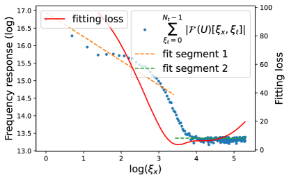
We find a transition frequency mode axsubscript𝑎𝑥{a_{x}} separating two regions (meaningful vs noise), by fitting a linear relation for low frequency modes (ξxaxsubscript𝜉𝑥subscript𝑎𝑥\xi_{x}\leq a_{x}), and fitting a flat line for high frequency modes (ξx>axsubscript𝜉𝑥subscript𝑎𝑥\xi_{x}>a_{x}) in the log\log-log\log scale:

ax=argminax{0,,Nx/2}Γ(ax),superscriptsubscript𝑎𝑥subscriptargminsubscript𝑎𝑥0subscript𝑁𝑥2Γsubscript𝑎𝑥\displaystyle a_{x}^{*}=\operatorname*{arg\,min}_{{a_{x}}\in\{0,...,\lfloor{N_{x}/2}\rfloor\}}\Gamma(a_{x}),
Γ(ax)=(mina,bξx{0,1,,ax}(alog(ξx)+blog[y(ξx)])2)+ξx=ax+1Nx/2(log[y¯(ax+1)]log[y(ξx)])2,Γsubscript𝑎𝑥subscript𝑎𝑏subscriptsubscript𝜉𝑥01subscript𝑎𝑥superscript𝑎subscript𝜉𝑥𝑏𝑦subscript𝜉𝑥2superscriptsubscriptsubscript𝜉𝑥subscript𝑎𝑥1subscript𝑁𝑥2superscript¯𝑦subscript𝑎𝑥1𝑦subscript𝜉𝑥2\displaystyle\Gamma(a_{x})=\left(\min_{a,b\in\mathbb{R}}\sum_{\xi_{x}\in\{0,1,...,{a_{x}}\}}\left(a\log(\xi_{x})+b-{\log[y(\xi_{x})]}\right)^{2}\right)+\sum_{\xi_{x}={a_{x}}+1}^{\lfloor{N_{x}/2}\rfloor}\left(\log[\bar{y}({a_{x}}+1)]-\log[y(\xi_{x})]\right)^{2}, (16)

with

y(ξx)=ξt=0Nt1|(U)[ξx,ξt]|,y¯(ax+1)=1Nx/2axξx=ax+1Nx/2ξt=0Nt1|(U)[ξx,ξt]|.formulae-sequence𝑦subscript𝜉𝑥superscriptsubscriptsubscript𝜉𝑡0subscript𝑁𝑡1𝑈subscript𝜉𝑥subscript𝜉𝑡¯𝑦subscript𝑎𝑥11subscript𝑁𝑥2subscript𝑎𝑥superscriptsubscriptsubscript𝜉𝑥subscript𝑎𝑥1subscript𝑁𝑥2superscriptsubscriptsubscript𝜉𝑡0subscript𝑁𝑡1𝑈subscript𝜉𝑥subscript𝜉𝑡\displaystyle y(\xi_{x})=\sum_{\xi_{t}=0}^{N_{t}-1}\big{|}\mathcal{F}(U)[\xi_{x},\xi_{t}]\big{|},\quad\bar{y}({a_{x}}+1)=\frac{1}{\lfloor{N_{x}/2}\rfloor-{a_{x}}}\sum_{\xi_{x}={a_{x}}+1}^{\lfloor{N_{x}/2}\rfloor}\sum_{\xi_{t}=0}^{N_{t}-1}\big{|}\mathcal{F}(U)[\xi_{x},\xi_{t}]\big{|}.

The first term in (16) fits the decay rate (15) and the second term fits the flat noise region. This is based on the assumption that low frequency data are dominated by the actual dynamics of the differential equation, while the high frequency data are mostly dominated by noise. Thus, a transition frequency mode can be detected by the change of the relation between log(ξt=0Nt1|((U))[ξx,ξt]|)superscriptsubscriptsubscript𝜉𝑡0subscript𝑁𝑡1𝑈subscript𝜉𝑥subscript𝜉𝑡\log\left(\sum_{\xi_{t}=0}^{N_{t}-1}\big{|}\mathcal{F}((U))[\xi_{x},\xi_{t}]\big{|}\right) and log(ξx)subscript𝜉𝑥\log(\xi_{x}). The transition frequency mode in time, denoted by atsuperscriptsubscript𝑎𝑡{a_{t}^{*}}, can be obtained similarly.

(a) (b)
Refer to caption Refer to caption
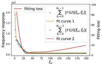
Figure 1: Decay fit in the frequency and physical domains. (a) Blue dots are the given data, orange and green dotted lines are the fitting lines to find the transition frequency mode axsuperscriptsubscript𝑎𝑥a_{x}^{*} (16) in log-log scale. (b) the same plot in physical domain and original unit. Red curves in both graphs show the fitting loss.

In Figure 1 (a) we show the accumulated frequency responses (blue dots), the linear fitting curve at the low-frequency modes (dash lines), and the total loss function ΓΓ\Gamma of (16) (red lines). The x𝑥x-axis and left-y𝑦y-axis provide the scales of points (xi,yi)subscript𝑥𝑖subscript𝑦𝑖(x_{i},y_{i}) in the linear fit. The right-y𝑦y-axis provides the scale of the loss function ΓΓ\Gamma in (16). In (b), visualization of the fitted curves is shown in the original scale (instead of log\log scale) in the frequency domain. The transition mode is detected as ax=27superscriptsubscript𝑎𝑥27a_{x}^{*}=27 from (16).

With the transition frequency modes axsuperscriptsubscript𝑎𝑥a_{x}^{*} and atsuperscriptsubscript𝑎𝑡a_{t}^{*} in ξxsubscript𝜉𝑥\xi_{x} and ξtsubscript𝜉𝑡\xi_{t} directions respectively, we partition the frequency domain into two regions: the meaningful data region ΛΛ\Lambda and noise regions, where

Λ={(ξx,ξt):ξx=0,1,,ax1,ξt=0,1,,at1}Λconditional-setsubscript𝜉𝑥subscript𝜉𝑡formulae-sequencesubscript𝜉𝑥01superscriptsubscript𝑎𝑥1subscript𝜉𝑡01superscriptsubscript𝑎𝑡1\Lambda=\{(\xi_{x},\xi_{t}):\xi_{x}=0,1,...,a_{x}^{*}-1,\xi_{t}=0,1,...,a_{t}^{*}-1\}

and the complement ΛsuperscriptΛcomplement\Lambda^{\complement} is the noise region. This is motivated from the theoretical decay rate of the Fourier coefficient of U𝑈U.

When the given data are noisy, each Fourier feature {gl}subscript𝑔𝑙\mathcal{F}\{g_{l}\} is also affected by noise. The region with a high response of {gl}subscript𝑔𝑙\mathcal{F}\{g_{l}\} usually contains more signal information than the region with a low response of {gl}subscript𝑔𝑙\mathcal{F}\{g_{l}\}. We further define the core region of feature for glsubscript𝑔𝑙g_{l}, denoted as 𝒱(gl)𝒱subscript𝑔𝑙\mathcal{V}(g_{l}) such that:

𝒱(gl)=(𝒱(gl),𝒱(gl)) with𝒱subscript𝑔𝑙subscript𝒱subscript𝑔𝑙subscript𝒱subscript𝑔𝑙 with\displaystyle\mathcal{V}(g_{l})=\left(\mathcal{V}_{\mathcal{R}}(g_{l}),\mathcal{V}_{\mathcal{I}}(g_{l})\right)\;\;\mbox{ with} (17)
𝒱(gl)={h=(ξx,ξt):(ξx,ξt)Λ,|([𝒮(𝑭)]h,l)|βgl},subscript𝒱subscript𝑔𝑙conditional-setsubscript𝜉𝑥subscript𝜉𝑡formulae-sequencesubscript𝜉𝑥subscript𝜉𝑡Λsubscriptdelimited-[]𝒮𝑭𝑙subscript𝛽subscript𝑔𝑙\displaystyle\mathcal{V}_{\mathcal{R}}(g_{l})=\left\{h=\mathcal{H}(\xi_{x},\xi_{t}):(\xi_{x},\xi_{t})\in\Lambda,\ |\mathcal{R}\left(\big{[}\mathcal{S}(\boldsymbol{F})\big{]}_{h,l}\right)|\geq\beta_{g_{l}}\right\},\ \
𝒱(gl)={h=(ξx,ξt):(ξx,ξt)Λ,|([𝒮(𝑭)]h,l)|βgl},subscript𝒱subscript𝑔𝑙conditional-setsubscript𝜉𝑥subscript𝜉𝑡formulae-sequencesubscript𝜉𝑥subscript𝜉𝑡Λsubscriptdelimited-[]𝒮𝑭𝑙subscript𝛽subscript𝑔𝑙\displaystyle\mathcal{V}_{\mathcal{I}}(g_{l})=\left\{h=\mathcal{H}(\xi_{x},\xi_{t}):(\xi_{x},\xi_{t})\in{\Lambda},\ |\mathcal{I}\left(\big{[}\mathcal{S}(\boldsymbol{F})\big{]}_{h,l}\right)|\geq\beta_{g_{l}}\right\},

where ()\mathcal{R}(\cdot) and ()\mathcal{I}(\cdot) denote the real part and imaginary part of its argument, respectively. Here 𝒱(gl)𝒱subscript𝑔𝑙\mathcal{V}(g_{l}) contains two ordered sets, in which the first set denotes the high response region for the real part of the Fourier feature for glsubscript𝑔𝑙g_{l}, and the second set denotes the high response region for the imaginary part.

For the feature glsubscript𝑔𝑙g_{l}, we pick the high responses among the frequencies in ΛΛ\Lambda to be in the core region of feature glsubscript𝑔𝑙g_{l}, and consider low responses as noise and remove them from the system (7). We refer to Subsection 5.2 for more details on how to choose the threshold βglsubscript𝛽subscript𝑔𝑙\beta_{g_{l}}. For the feature utsubscript𝑢𝑡u_{t}, we consider the smoothed frequency response restricted to ΛΛ\Lambda, 𝒮(𝒃)Λ𝒮subscript𝒃Λ\mathcal{S}({\boldsymbol{b}})_{\Lambda}, and its magnitude at each frequency. We take the high response region as the core region determined by a threshold βutsubscript𝛽subscript𝑢𝑡\beta_{u_{t}}. Specifically, the core region of utsubscript𝑢𝑡u_{t}, 𝒱(ut)𝒱subscript𝑢𝑡\mathcal{V}(u_{t}), is defined similarly as 𝒱(gl)𝒱subscript𝑔𝑙\mathcal{V}(g_{l}) in (17), where βglsubscript𝛽subscript𝑔𝑙\beta_{g_{l}} is replaced by βutsubscript𝛽subscript𝑢𝑡\beta_{u_{t}} and 𝒮(𝑭)h,l𝒮subscript𝑭𝑙\mathcal{S}(\boldsymbol{F})_{h,l} is replaced by 𝒮(𝒃)h𝒮subscript𝒃\mathcal{S}(\boldsymbol{b})_{h}.

Using the core region of feature utsubscript𝑢𝑡u_{t}, we construct the linear system as

𝒮(𝑭)𝒱(ut)¯𝒄=𝒮(𝒃)𝒱(ut)¯,¯𝒮subscript𝑭𝒱subscript𝑢𝑡𝒄¯𝒮subscript𝒃𝒱subscript𝑢𝑡\overline{\mathcal{S}({\boldsymbol{F}})_{\mathcal{V}(u_{t})}}\boldsymbol{c}=\overline{\mathcal{S}({\boldsymbol{b}})_{\mathcal{V}(u_{t})}}, (18)

where

𝒮(𝑭)𝒱(ut)¯=[(𝒮(𝑭)𝒱(ut))(𝒮(𝑭)𝒱(ut))]and𝒮(𝒃)𝒱(ut)¯=[(𝒮(𝒃)𝒱(ut))(𝒮(𝒃)𝒱(ut))].¯𝒮subscript𝑭𝒱subscript𝑢𝑡matrix𝒮subscript𝑭subscript𝒱subscript𝑢𝑡𝒮subscript𝑭subscript𝒱subscript𝑢𝑡and¯𝒮subscript𝒃𝒱subscript𝑢𝑡matrix𝒮subscript𝒃subscript𝒱subscript𝑢𝑡𝒮subscript𝒃subscript𝒱subscript𝑢𝑡\overline{\mathcal{S}({\boldsymbol{F}})_{\mathcal{V}({u_{t}})}}=\begin{bmatrix}\mathcal{R}\left(\mathcal{S}(\boldsymbol{F})_{\mathcal{V}_{\mathcal{R}}(u_{t})}\right)\\ \mathcal{I}\left(\mathcal{S}(\boldsymbol{F})_{\mathcal{V}_{\mathcal{I}}(u_{t})}\right)\end{bmatrix}\;\;\text{and}\;\;\overline{\mathcal{S}({\boldsymbol{b}})_{\mathcal{V}({u_{t}})}}=\begin{bmatrix}\mathcal{R}\left(\mathcal{S}(\boldsymbol{b})_{\mathcal{V}_{\mathcal{R}}(u_{t})}\right)\\ \mathcal{I}\left(\mathcal{S}(\boldsymbol{b})_{\mathcal{V}_{\mathcal{I}}(u_{t})}\right)\end{bmatrix}.

Here we use 𝒮(𝑭)𝒱(ut)𝒮subscript𝑭subscript𝒱subscript𝑢𝑡\mathcal{S}(\boldsymbol{F})_{\mathcal{V}_{\mathcal{R}}(u_{t})} to denote the submatrix of 𝒮(𝑭)𝒮𝑭\mathcal{S}(\boldsymbol{F}) with rows restricted to the ones indexed by 𝒱(ut)subscript𝒱subscript𝑢𝑡{\mathcal{V}_{\mathcal{R}}(u_{t})}. The overline denotes the vertical stacking of real and imaginary responses. This leads to a reduced linear system (18) that is defined only on the core region of the feature utsubscript𝑢𝑡u_{t}. We represent the coefficients identified within the core region of utsubscript𝑢𝑡u_{t} as

𝒄𝒱(ut)=LeastSquare(𝒮(𝐅)𝒱(ut)~,𝒮(𝐛)𝒱(ut)~).subscript𝒄𝒱subscript𝑢𝑡LeastSquare~𝒮subscript𝐅𝒱subscriptut~𝒮subscript𝐛𝒱subscriptut\boldsymbol{c}_{\mathcal{V}(u_{t})}=\rm{LeastSquare}(\widetilde{\mathcal{S}(\boldsymbol{F})_{\mathcal{V}(u_{t})}},\widetilde{\mathcal{S}(\boldsymbol{b})_{\mathcal{V}(u_{t})}}). (19)

Here we use the error-normalized Fourier feature matrix 𝒮(𝑭)𝒱(ut)~~𝒮subscript𝑭𝒱subscript𝑢𝑡\widetilde{\mathcal{S}(\boldsymbol{F})_{\mathcal{V}(u_{t})}} and the error-normalized dynamic variable 𝒮(𝒃)𝒱(ut)~~𝒮subscript𝒃𝒱subscript𝑢𝑡\widetilde{\mathcal{S}(\boldsymbol{b})_{\mathcal{V}(u_{t})}} defined in (33) to solve the least square problem in (19) (details presented in Subsection 5.3).

4 Fourier features for Identifying differential equations (FourierIdent)

Construct the Fourier system (7), from the given data 𝒟𝒟\mathcal{D} (4). [Step 1] Fourier feature denoising and construct 𝒮(𝑭)𝒱(ut)¯¯𝒮subscript𝑭𝒱subscript𝑢𝑡\overline{\mathcal{S}(\boldsymbol{F})_{\mathcal{V}(u_{t})}} and 𝒮(𝒃)𝒱(ut)¯¯𝒮subscript𝒃𝒱subscript𝑢𝑡\overline{\mathcal{S}(\boldsymbol{b})_{\mathcal{V}(u_{t})}} in (18). [Step 2] For k=1,2,,K𝑘12𝐾k=1,2,...,K, apply SP and group trimming to obtain the support 𝒜ksubscript𝒜𝑘\mathcal{A}_{k}. [Step 3] Chose the best sparsity ksuperscript𝑘k^{*} as in (25), and use 𝒱superscript𝒱\mathcal{V}^{*} in (26) to compute the coefficient 𝒄𝒱subscript𝒄superscript𝒱\boldsymbol{c}_{\mathcal{V}^{*}}. Output 𝒄𝒱subscript𝒄superscript𝒱\boldsymbol{c}_{\mathcal{V}^{*}}
Figure 2: The flowchart of FourierIdent. A discrete Fourier system (7) is constructed from the given data. In [Step 1], Fourier features are denoised and a smaller system (18) is constructed. In [Step 2], we apply Subspace Pursuit to obtain initial supports for each sparsity level k=1,2,,K𝑘12𝐾k=1,2,...,K and new group trimming is applied. In [Step 3], the best coefficient is computed from the energy (25) based on core region.

From the given data, Fourier features are denoised and a smaller linear system with reduced size is constructed in Section 3. We utilize Subspace Pursuit [6] for the coefficient support identification, and we propose (i) a new group trimming for stable support recovery, and (ii) a new energy based on the core regions of features for the coefficient identification. There are three steps to the proposed FourierIdent, and Figure 2 shows the flowchart to illustrate the process.

  1. 1.

    From the given input data, we construct a denoised linear system with 𝒮(𝑭)𝒱(ut)¯¯𝒮subscript𝑭𝒱subscript𝑢𝑡\overline{\mathcal{S}(\boldsymbol{F})_{\mathcal{V}(u_{t})}} and 𝒮(𝒃)𝒱(ut)¯¯𝒮subscript𝒃𝒱subscript𝑢𝑡\overline{\mathcal{S}(\boldsymbol{b})_{\mathcal{V}(u_{t})}} in (18). This is generated by the denoising operation 𝒮𝒮\mathcal{S} in (13), the discrete Fourier system (7) and using the core region of utsubscript𝑢𝑡u_{t}, 𝒱(ut)𝒱subscript𝑢𝑡\mathcal{V}(u_{t}), to reduce the size and denoise the system.

  2. 2.

    For each sparsity level k=1,2,,K𝑘12𝐾k=1,2,\dots,K, we apply Subspace Pursuit [6] on a column normalized system of 𝒮(𝑭)𝒱(ut)¯superscript¯𝒮subscript𝑭𝒱subscript𝑢𝑡\overline{\mathcal{S}({\boldsymbol{F}})_{\mathcal{V}(u_{t})}}^{\dagger}, and 𝒮(𝒃)𝒱(ut)¯superscript¯𝒮subscript𝒃𝒱subscript𝑢𝑡\overline{\mathcal{S}({\boldsymbol{b}})_{\mathcal{V}(u_{t})}}^{\dagger} and get an initial support 𝒜k0superscriptsubscript𝒜𝑘0\mathcal{A}_{k}^{0}. (Here denotes the column normalization, which each column is normalized independently.) We apply a new group trimming to remove features which minimally contribute to the dynamics of the system. This is applied iteratively, until the support converges to 𝒜ksubscript𝒜𝑘\mathcal{A}_{k} for each k𝑘k.

  3. 3.

    To choose the optimal coefficient, we propose a new energy based on the core regions of features. First, the optimal sparsity is determined by choosing ksuperscript𝑘k^{*} which gives the minimum residual on the union of the core regions of features identified in 𝒜ksubscript𝒜𝑘\mathcal{A}_{k}. Secondly, we identify the optimal coefficients, by finding the coefficients which gives the minimum residual among least-square fits on the core region of each feature in 𝒜ksubscript𝒜𝑘\mathcal{A}_{k}.

  Input: Given data (4).
  [Step 1] Construct the discrete linear system 𝒮(𝑭)¯𝒱(ut),𝒮(𝒃)¯𝒱(ut)subscript¯𝒮𝑭𝒱subscript𝑢𝑡subscript¯𝒮𝒃𝒱subscript𝑢𝑡\overline{\mathcal{S}({\boldsymbol{F}})}_{\mathcal{V}(u_{t})},\overline{\mathcal{S}({\boldsymbol{b}})}_{\mathcal{V}(u_{t})} as in (18).
  [Step 2]
  for k = 1,2,…,K do
     Run SP(𝒮(𝑭)𝒱(ut)¯,𝒮(𝒃)𝒱(ut)¯,k)superscript¯𝒮subscript𝑭𝒱subscript𝑢𝑡superscript¯𝒮subscript𝒃𝒱subscript𝑢𝑡𝑘(\overline{\mathcal{S}({\boldsymbol{F}})_{\mathcal{V}(u_{t})}}^{\dagger},\overline{\mathcal{S}({\boldsymbol{b}})_{\mathcal{V}(u_{t})}}^{\dagger},k)  using SP [6] and set j=0𝑗0j=0 ;
      Compute the coefficients 𝒄𝒱(ut)subscript𝒄𝒱subscript𝑢𝑡\boldsymbol{c}_{\mathcal{V}(u_{t})} by the Least Square in (19);
     while 𝒜kjsuperscriptsubscript𝒜𝑘𝑗\mathcal{A}_{k}^{j} not convergent  do
         Perform group trimming in (21) with 𝒯=0.08𝒯0.08\mathcal{T}=0.08 and set j=j+1𝑗𝑗1j=j+1 ;
         Update the contribution score slsubscript𝑠𝑙s_{l} in (20), using the updated coefficients 𝒄𝒱(ut)subscript𝒄𝒱subscript𝑢𝑡\boldsymbol{c}_{\mathcal{V}(u_{t})} in (19);
     end while
  end for
  [Step 3 - 1] Determine the optimal sparsity ksuperscript𝑘k^{*} according to (25) and the support 𝒜ksubscript𝒜superscript𝑘\mathcal{A}_{k^{*}}.
  [Step 3 - 2] Compute 𝒄superscript𝒄\boldsymbol{c}^{*} by minimizing (27).
  Output: 𝒄Lsuperscript𝒄superscript𝐿\boldsymbol{c}^{*}\in\mathbb{R}^{L} such that 𝑭𝒄𝒃𝑭superscript𝒄𝒃\boldsymbol{F}\boldsymbol{c}^{*}\approx\boldsymbol{b} .
Algorithm 1 FourierIdent Algorithm

4.1 Subspace Pursuit (SP) and Group trimming in [Step 2]

With the denoised Fourier features, we apply Subspace Pursuit (SP) [6] to obtain an initial support Ak0superscriptsubscript𝐴𝑘0A_{k}^{0} with each sparsity level k𝑘k. The goal is to find a k𝑘k-sparse solution of the linear system Φ𝒙=𝒃Φ𝒙𝒃\Phi\boldsymbol{x}=\boldsymbol{b}:

min𝒙:𝒙0=kΦ𝒙𝒃22.subscript:𝒙subscriptnorm𝒙0𝑘superscriptsubscriptnormΦ𝒙𝒃22\displaystyle\min_{\boldsymbol{x}:\|\boldsymbol{x}\|_{0}=k}\|\Phi\boldsymbol{x}-\boldsymbol{b}\|_{2}^{2}.

One inputs a column normalized matrix ΦΦ\Phi, a vector 𝒃𝒃\boldsymbol{b}, and a sparsity k𝑘k, and Subspace Pursuit SP(Φ,𝒃,k)SPΦ𝒃𝑘{\rm SP}(\Phi,\boldsymbol{b},k) outputs a k𝑘k-sparse solution in a greedy way (See [6] for details).

For each sparsity level k=1,,K𝑘1𝐾k=1,\dots,K, we compute SP(𝒮(𝑭)𝒱(ut)¯,𝒮(𝒃)𝒱(ut)¯,k)SPsuperscript¯𝒮subscript𝑭𝒱subscript𝑢𝑡superscript¯𝒮subscript𝒃𝒱subscript𝑢𝑡𝑘{\rm SP}(\overline{\mathcal{S}({\boldsymbol{F}})_{\mathcal{V}(u_{t})}}^{\dagger},\overline{\mathcal{S}({\boldsymbol{b}})_{\mathcal{V}(u_{t})}}^{\dagger},k), and denote the recovered support as Ak0subscriptsuperscript𝐴0𝑘A^{0}_{k}. To further remove the insignificant features in Ak0superscriptsubscript𝐴𝑘0A_{k}^{0}, we trim the features which have minimum contributions to the dynamics, measured by the contribution score;

sl=s(gl)=|cl|𝒮(𝑭)𝒱(ut),l¯2.subscript𝑠𝑙𝑠subscript𝑔𝑙subscript𝑐𝑙subscriptnorm¯𝒮subscript𝑭𝒱subscript𝑢𝑡𝑙2s_{l}=s(g_{l})=|c_{l}|\cdot\|\overline{\mathcal{S}(\boldsymbol{F})_{\mathcal{V}(u_{t}),l}}\|_{2}\;. (20)

Here 𝒮(𝑭)𝒱(ut),l¯¯𝒮subscript𝑭𝒱subscript𝑢𝑡𝑙\overline{\mathcal{S}(\boldsymbol{F})_{\mathcal{V}(u_{t}),l}} is the l𝑙l-th column of 𝒮(𝑭)¯¯𝒮𝑭\overline{\mathcal{S}(\boldsymbol{F})} with rows restricted to the core region 𝒱(ut)𝒱subscript𝑢𝑡\mathcal{V}(u_{t}). The value clsubscript𝑐𝑙c_{l} is the l𝑙l-th entry of the identified coefficient from the least-square fit of 𝒮(𝑭)𝒱(ut)¯¯𝒮subscript𝑭𝒱subscript𝑢𝑡\overline{\mathcal{S}({\boldsymbol{F}})_{\mathcal{V}(u_{t})}} and 𝒮(𝒃)𝒱(ut)¯¯𝒮subscript𝒃𝒱subscript𝑢𝑡\overline{\mathcal{S}({\boldsymbol{b}})_{\mathcal{V}(u_{t})}}.

To improve the efficiency of the algorithm, we propose to trim features as a group. We remove a set of the least relevant features for a given sparsity level k𝑘k using a threshold 𝒯𝒯\mathcal{T}. In this paper, we fix this threshold to be 𝒯=0.008𝒯0.008\mathcal{T}=0.008. The group-trimming is used as follows:

  • Re-order features by contribution scores. We arrange the features in ascending order, denoted as 1,2,,ksuperscript1superscript2superscript𝑘1^{\prime},2^{\prime},...,k^{\prime}, based on their respective contribution scores, represented as s1s2sksubscript𝑠superscript1subscript𝑠superscript2subscript𝑠superscript𝑘s_{1^{\prime}}\leq s_{2^{\prime}}\leq...\leq s_{k^{\prime}}.

  • Remove the low contributing terms as a group. We identify the largest value kmaxsuperscriptsubscript𝑘k_{\max}^{\prime} satisfying condition

    j=1kmaxsjk𝒜k0sk<𝒯j=1kmax+1sjk𝒜k0sk,superscriptsubscript𝑗superscript1superscriptsubscript𝑘subscript𝑠𝑗subscript𝑘superscriptsubscript𝒜𝑘0subscript𝑠𝑘𝒯superscriptsubscript𝑗superscript1superscriptsubscript𝑘1subscript𝑠𝑗subscript𝑘superscriptsubscript𝒜𝑘0subscript𝑠𝑘\frac{\sum_{j=1^{\prime}}^{k_{\max}^{\prime}}s_{j}}{\sum_{k\in\mathcal{A}_{k}^{0}}s_{k}}<\mathcal{T}\leq\frac{\sum_{j=1^{\prime}}^{k_{\max}^{\prime}+1}s_{j}}{\sum_{k\in\mathcal{A}_{k}^{0}}s_{k}}, (21)

    and remove features with contribution scores equal to or lower than skmaxsubscript𝑠superscriptsubscript𝑘s_{k_{\max}^{\prime}}, i.e., slskmaxsubscript𝑠𝑙subscript𝑠superscriptsubscript𝑘s_{l}\leq s_{k_{\max}^{\prime}} from the support set 𝒜kisuperscriptsubscript𝒜𝑘𝑖\mathcal{A}_{k}^{i} when kmax>0superscriptsubscript𝑘0k_{\max}^{\prime}>0, where 𝒜kisuperscriptsubscript𝒜𝑘𝑖\mathcal{A}_{k}^{i} denotes the support at the i𝑖ith iteration after the i𝑖ith group trimming. This step reduces the size of the support and the support becomes 𝒜ki+1superscriptsubscript𝒜𝑘𝑖1\mathcal{A}_{k}^{i+1}. Here 𝒯𝒯\mathcal{T} helps to remove a subgroup of features that contributes less than a threshold (which is set to be 8% in this paper) overall compared to all features in the support 𝒜kisuperscriptsubscript𝒜𝑘𝑖\mathcal{A}_{k}^{i}. This 𝒯𝒯\mathcal{T} is a measure of the relative significance of a smaller subgroup of trimmed features compared to the whole set of features.

  • Trimming in each iteration. This group trimming is applied iteratively within each sparsity level k𝑘k, and the converged support set is assigned as 𝒜ksubscript𝒜𝑘\mathcal{A}_{k}. Note that equation (21) changes in each iteration and must be recomputed.

The group trimming is a grouped version of trimming introduced in WeakIdent [30]. The group trimming improves efficiency by removing insignificant terms as a group and gives stable results for different types of equations with various levels of noise.

4.2 Identification of coefficients from the core regions of features in [Step 3]

Once we have a collection of support sets 𝒜ksubscript𝒜𝑘\mathcal{A}_{k}’s for k=1,,K𝑘1𝐾k=1,\dots,K, we choose the optimal sparsity ksuperscript𝑘k^{*} (and the associated support 𝒜ksubscript𝒜superscript𝑘\mathcal{A}_{k^{*}}) which minimizes an energy based on the core regions of features. This energy consists of two terms:

Energy =Fitting residual on the union of core regions in 𝒜k1+ Stability of the identified coefficient2.absentsubscriptFitting residual on the union of core regions in subscript𝒜𝑘subscript1subscript Stability of the identified coefficientsubscript2\displaystyle=\underbrace{\text{Fitting residual on the union of core regions in }\mathcal{A}_{k}}_{\mathcal{E}_{1}}+\underbrace{\text{ Stability of the identified coefficient}}_{\mathcal{E}_{2}}. (22)

The first term 1subscript1\mathcal{E}_{1} is the fitting residual at the frequencies on the union of the core regions for the features in 𝒜ksubscript𝒜𝑘\mathcal{A}_{k}:

1:=𝒮(𝑭)𝒱(𝒜k)𝒄𝒱(𝒜k)𝒮(𝒃)𝒱(𝒜k)2𝒮(𝒃)𝒱(𝒜k)2.assignsubscript1subscriptnorm𝒮subscript𝑭𝒱subscript𝒜𝑘subscript𝒄𝒱subscript𝒜𝑘𝒮subscript𝒃𝒱subscript𝒜𝑘2subscriptnorm𝒮subscript𝒃𝒱subscript𝒜𝑘2\mathcal{E}_{1}:=\frac{\|{\mathcal{S}(\boldsymbol{F})_{\mathcal{V}({\mathcal{A}_{k}})}}{{\boldsymbol{c}_{\mathcal{V}({\mathcal{A}_{k}})}}}-{\mathcal{S}(\boldsymbol{b})_{\mathcal{V}({\mathcal{A}_{k}})}}\|_{2}}{\|{\mathcal{S}(\boldsymbol{b})_{\mathcal{V}({\mathcal{A}_{k}})}}\|_{2}}. (23)

Here 𝒄𝒱(𝒜k)subscript𝒄𝒱subscript𝒜𝑘{\boldsymbol{c}_{\mathcal{V}({\mathcal{A}_{k}})}} denotes the coefficients recovered using an error-normalized feature matrix 𝒮(𝑭)𝒱(ut)~~𝒮subscript𝑭𝒱subscript𝑢𝑡\widetilde{\mathcal{S}(\boldsymbol{F})_{\mathcal{V}(u_{t})}} and dynamic variable 𝒮(𝒃)𝒱(ut)~~𝒮subscript𝒃𝒱subscript𝑢𝑡\widetilde{\mathcal{S}(\boldsymbol{b})_{\mathcal{V}(u_{t})}} defined in (33) in Subsection 5.3. The union of core regions for the features in 𝒜ksubscript𝒜𝑘\mathcal{A}_{k} is

𝒱(𝒜k)=l𝒜k𝒱(gl).𝒱subscript𝒜𝑘subscript𝑙subscript𝒜𝑘𝒱subscript𝑔𝑙\mathcal{V}(\mathcal{A}_{k})=\bigcup_{l\in\mathcal{A}_{k}}\mathcal{V}(g_{l}).

While each feature gives different core regions (high response regions), by using the union 𝒱(𝒜k)𝒱subscript𝒜𝑘\mathcal{V}(\mathcal{A}_{k}), we consider fitting on the high response regions for all the features in 𝒜ksubscript𝒜𝑘\mathcal{A}_{k}

The second term in (22) measures the stability of the identified coefficients. For each feature glsubscript𝑔𝑙g_{l} such that l𝒜k𝑙subscript𝒜𝑘l\in\mathcal{A}_{k}, we compute the coefficients 𝒄𝒱(gl)subscript𝒄𝒱subscript𝑔𝑙\boldsymbol{c}_{\mathcal{V}(g_{l})} as in (19) while the core region 𝒱(ut)𝒱subscript𝑢𝑡\mathcal{V}(u_{t}) is replaced by 𝒱(gl)𝒱subscript𝑔𝑙\mathcal{V}(g_{l}). We compare the normalized distance among all coefficient vectors computed on the core region of each feature in 𝒜ksubscript𝒜𝑘\mathcal{A}_{k}, and define the follwing stability term:

2:=1|𝒜k|21𝒄𝒱(ut)2l,l𝒜k,ll𝒄𝒱(gl)𝒄𝒱(gl)2.assignsubscript21superscriptsubscript𝒜𝑘21subscriptnormsubscript𝒄𝒱subscript𝑢𝑡2subscriptformulae-sequence𝑙superscript𝑙subscript𝒜𝑘𝑙superscript𝑙subscriptnormsubscript𝒄𝒱subscript𝑔𝑙subscript𝒄𝒱subscript𝑔superscript𝑙2\mathcal{E}_{2}:=\frac{1}{\big{|}\mathcal{A}_{k}\big{|}^{2}}\frac{1}{\big{\|}\boldsymbol{c}_{\mathcal{V}(u_{t})}\big{\|}_{2}}\sum_{l,l^{\prime}\in\mathcal{A}_{k},l\neq l^{\prime}}\big{\|}\boldsymbol{c}_{\mathcal{V}(g_{l})}-\boldsymbol{c}_{\mathcal{V}(g_{l^{\prime}})}\big{\|}_{2}. (24)

If fitting on the core region of one feature gives a very different coefficient vector from fitting on the core region of another feature, this stability term in (24) will be larger than when the coefficients computed on the core regions of different features are similar. This term measures the stability of coefficient computation on the core regions of different features in 𝒜ksubscript𝒜𝑘\mathcal{A}_{k}.

We find the optimal sparsity ksuperscript𝑘k^{*} and the associated support set 𝒜ksubscript𝒜superscript𝑘\mathcal{A}_{k^{*}} by minimizing the energy 1+2subscript1subscript2\mathcal{E}_{1}+\mathcal{E}_{2}:

k=argmink{𝒮(𝑭)𝒱(𝒜k)𝒄𝒱(𝒜k)𝒮(𝒃)𝒱(𝒜k)2𝒮(𝒃)𝒱(𝒜k)2+1|𝒜k|21𝒄𝒱(ut)2l,l𝒜k,ll𝒄𝒱(gl)𝒄𝒱(gl)2}.superscript𝑘subscriptargmin𝑘subscriptnorm𝒮subscript𝑭𝒱subscript𝒜𝑘subscript𝒄𝒱subscript𝒜𝑘𝒮subscript𝒃𝒱subscript𝒜𝑘2subscriptnorm𝒮subscript𝒃𝒱subscript𝒜𝑘21superscriptsubscript𝒜𝑘21subscriptnormsubscript𝒄𝒱subscript𝑢𝑡2subscriptformulae-sequence𝑙superscript𝑙subscript𝒜𝑘𝑙superscript𝑙subscriptnormsubscript𝒄𝒱subscript𝑔𝑙subscript𝒄𝒱subscript𝑔superscript𝑙2k^{*}=\operatorname*{arg\,min}_{k}\left\{\frac{\|{\mathcal{S}(\boldsymbol{F})_{\mathcal{V}({\mathcal{A}_{k}})}}{\boldsymbol{c}_{\mathcal{V}({\mathcal{A}_{k}})}}-{\mathcal{S}(\boldsymbol{b})_{\mathcal{V}({\mathcal{A}_{k}})}}\|_{2}}{\|{\mathcal{S}(\boldsymbol{b})_{\mathcal{V}({\mathcal{A}_{k}})}}\|_{2}}+\frac{1}{\big{|}\mathcal{A}_{k}\big{|}^{2}}\frac{1}{\big{\|}\boldsymbol{c}_{\mathcal{V}(u_{t})}\big{\|}_{2}}\sum_{l,l^{\prime}\in\mathcal{A}_{k},l\neq l^{\prime}}\big{\|}\boldsymbol{c}_{\mathcal{V}(g_{l})}-\boldsymbol{c}_{\mathcal{V}(g_{l^{\prime}})}\big{\|}_{2}\right\}. (25)

The energy summing (23) and (24) measures how meaningful the recovered support 𝒜ksubscript𝒜𝑘\mathcal{A}_{k} is in terms of the best fitting on the union of core regions and the stability of coefficient identification.

Finally, we compute the best coefficient vector 𝒄superscript𝒄\boldsymbol{c}^{*} by solving a least square problem on a properly selected core region, that gives the smallest residual among the features in 𝒜ksubscript𝒜superscript𝑘\mathcal{A}_{k^{*}} and utsubscript𝑢𝑡u_{t}. For each core region of each features in 𝒜ksubscript𝒜superscript𝑘\mathcal{A}_{k^{*}} and utsubscript𝑢𝑡u_{t}, residual error is computed. Let 𝒱superscript𝒱\mathcal{V}^{*} be the best core region of features among all features in 𝒜ksubscript𝒜superscript𝑘\mathcal{A}_{k^{*}} and utsubscript𝑢𝑡u_{t}, which gives the minimum residual:

𝒱=argminV{𝒱(ut),𝒱(gl):l𝒜k}𝒮(𝑭)V𝒄V𝒮(𝒃)V2𝒮(𝒃)V2.superscript𝒱subscriptargmin𝑉conditional-set𝒱subscript𝑢𝑡𝒱subscript𝑔𝑙𝑙subscript𝒜superscript𝑘subscriptnorm𝒮subscript𝑭𝑉subscript𝒄𝑉𝒮subscript𝒃𝑉2subscriptnorm𝒮subscript𝒃𝑉2\mathcal{V}^{*}=\operatorname*{arg\,min}_{V\in\big{\{}\mathcal{V}(u_{t}),\mathcal{V}({g_{l}}):l\in\mathcal{A}_{k^{*}}\big{\}}}\frac{\|\mathcal{S}(\boldsymbol{F})_{V}\boldsymbol{c}_{V}-\mathcal{S}(\boldsymbol{b})_{V}\|_{2}}{\|\mathcal{S}(\boldsymbol{b})_{V}\|_{2}}. (26)

The core regions for each feature in 𝒜ksubscript𝒜superscript𝑘\mathcal{A}_{k^{*}} and utsubscript𝑢𝑡u_{t} are used to find the minimum residual in (26) such that V{𝒱(ut),𝒱(gl):l𝒜k}𝑉conditional-set𝒱subscript𝑢𝑡𝒱subscript𝑔𝑙𝑙subscript𝒜superscript𝑘V\in\big{\{}\mathcal{V}(u_{t}),\mathcal{V}({g_{l}}):l\in\mathcal{A}_{k^{*}}\big{\}}. In our experiments, using the union 𝒱(𝒜k)𝒱subscript𝒜superscript𝑘\mathcal{V}(\mathcal{A}_{k^{*}}) does not give good results. When fewer number of features are used for the core region, it gives better coefficient recovery. In (26), we experiment on the core regions for each feature, and pick one feature to define the core region.

With 𝒱superscript𝒱\mathcal{V}^{*}, the identified coefficient vector 𝒄superscript𝒄\boldsymbol{c}^{*} is given by

𝒄=LeastSquare(𝒮(𝐅)𝒱~,𝒮(𝐛)𝒱~)superscript𝒄LeastSquare~𝒮subscript𝐅superscript𝒱~𝒮subscript𝐛superscript𝒱\boldsymbol{c}^{*}=\rm{LeastSquare}(\widetilde{\mathcal{S}(\boldsymbol{F})_{\mathcal{V}^{*}}},\widetilde{\mathcal{S}(\boldsymbol{b})_{\mathcal{V}^{*}}}) (27)

using error-normalized feature matrix 𝒮(𝑭)𝒱~~𝒮subscript𝑭superscript𝒱\widetilde{{\mathcal{S}(\boldsymbol{F})_{\mathcal{V}^{*}}}} and dynamic variable 𝒮(𝒃)𝒱~~𝒮subscript𝒃superscript𝒱\widetilde{{\mathcal{S}(\boldsymbol{b})_{\mathcal{V}^{*}}}} as defined in (33).

5 Numerical Implementation Details

We present implementation details in this section. First, we propose a method to extend and augment the data when the given data are not periodic. Secondly, we discuss the details of how the threshold is computed for the core regions of features. Thirdly, we review the details of error-normalization on how it is applied in the frequency domain.

5.1 Domain extension for different boundary conditions

Applying the Fourier Transform on u𝑢u requires u𝑢u to be periodic along both t𝑡t and x𝑥x directions. When u(x,t)𝑢𝑥𝑡u(x,t) does not satisfy this periodic condition, we extend it to a periodic function to compute Fourier coefficients.

We introduce two transformation operators tsubscript𝑡\mathcal{H}_{t} and 𝒢tsubscript𝒢𝑡\mathcal{G}_{t} defined as follows:

𝒢t(fl(u(x,t)))={fl(u(x,t))0xX,0tT,fl(u(x,2Tt))0xX,Tt2T,subscript𝒢𝑡subscript𝑓𝑙𝑢𝑥𝑡casessubscript𝑓𝑙𝑢𝑥𝑡formulae-sequence0𝑥𝑋0𝑡𝑇subscript𝑓𝑙𝑢𝑥2𝑇𝑡formulae-sequence0𝑥𝑋𝑇𝑡2𝑇{\mathcal{G}_{t}(f_{l}(u(x,t)))}=\begin{cases}f_{l}(u(x,t))&0\leq x\leq X,0\leq t\leq T,\\ -f_{l}(u(x,2T-t))&0\leq x\leq X,T\leq t\leq 2T,\\ \end{cases}

and

t(u(x,t))={u(x,t)0xX,0tT,u(x,2Tt)0xX,Tt2T,subscript𝑡𝑢𝑥𝑡cases𝑢𝑥𝑡formulae-sequence0𝑥𝑋0𝑡𝑇𝑢𝑥2𝑇𝑡formulae-sequence0𝑥𝑋𝑇𝑡2𝑇{\mathcal{H}_{t}(u(x,t))}=\begin{cases}u(x,t)&0\leq x\leq X,0\leq t\leq T,\\ u(x,2T-t)&0\leq x\leq X,T\leq t\leq 2T,\\ \end{cases}

where u(x,t)𝑢𝑥𝑡u(x,t) is a continues function for x[0,X]𝑥0𝑋x\in[0,X] and t[0,T]𝑡0𝑇t\in[0,T]. The subscript t𝑡t denotes that we are extending u(x,t)𝑢𝑥𝑡u(x,t) along t𝑡t. One can easily check that both extended functions 𝒢t(u(x,t))subscript𝒢𝑡𝑢𝑥𝑡{\mathcal{G}_{t}(u(x,t))} and t(u(x,t))subscript𝑡𝑢𝑥𝑡{\mathcal{H}_{t}(u(x,t))} are periodic along t𝑡t. Then the equation (5) is converted to an alternative form

t(u)t(x,t)=l=1Lclαl𝒢t(fl(u))xαl,subscript𝑡𝑢𝑡𝑥𝑡superscriptsubscript𝑙1𝐿subscript𝑐𝑙superscriptsubscript𝛼𝑙subscript𝒢𝑡subscript𝑓𝑙𝑢superscript𝑥subscript𝛼𝑙\displaystyle\frac{\partial\mathcal{H}_{t}(u)}{\partial t}(x,t)=\sum_{l=1}^{L}c_{l}\frac{\partial^{\alpha_{l}}\mathcal{G}_{t}(f_{l}(u))}{\partial x^{\alpha_{l}}}, (28)

where utsubscript𝑢𝑡u_{t} is computed with t(Unoise,in)subscript𝑡superscriptsubscript𝑈𝑛𝑜𝑖𝑠𝑒𝑖𝑛\mathcal{H}_{t}(U_{noise,i}^{n}) instead of Unoise,insuperscriptsubscript𝑈𝑛𝑜𝑖𝑠𝑒𝑖𝑛U_{noise,i}^{n} and features on the right-hand side are computed using 𝒢t(fl(Unoise,in))subscript𝒢𝑡subscript𝑓𝑙superscriptsubscript𝑈𝑛𝑜𝑖𝑠𝑒𝑖𝑛\mathcal{G}_{t}(f_{l}(U_{noise,i}^{n})). For simplification of notation, we present the paper with Unoise,insuperscriptsubscript𝑈𝑛𝑜𝑖𝑠𝑒𝑖𝑛U_{noise,i}^{n}. However, when the given data do not satisfy the period boundary condition, we consistently use the extended boundary equation (28) instead of (5).

5.2 Threshold computation for the core region of features

We present how the threshold βutsubscript𝛽subscript𝑢𝑡\beta_{u_{t}} used in Subsection 3.2 is chosen to determine the core region of feature for utsubscript𝑢𝑡u_{t}. In Subsection 3.2, we partition the meaningful data region ΛΛ\Lambda further into the core region (high response region of the feature), and the noise region (low response region of the feature). The partition is based on the threshold βutsubscript𝛽subscript𝑢𝑡\beta_{u_{t}}.

  1. 1.

    First, we collect absolute values of the smoothed responses for utsubscript𝑢𝑡u_{t} in ΛΛ\Lambda in a new set denoted by \mathcal{B}. We take the absolute values of both the real and imaginary parts for each index h=(ξx,ξt)subscript𝜉𝑥subscript𝜉𝑡h=\mathcal{H}(\xi_{x},\xi_{t}). Here the frequency index h=(ξx,ξt)subscript𝜉𝑥subscript𝜉𝑡h=\mathcal{H}(\xi_{x},\xi_{t}) is in the meaningful data region ΛΛ\Lambda such that ξx=1,,axsubscript𝜉𝑥1superscriptsubscript𝑎𝑥\xi_{x}=1,\ldots,a_{x}^{*} and ξt=1,,atsubscript𝜉𝑡1superscriptsubscript𝑎𝑡\xi_{t}=1,\ldots,a_{t}^{*}.

  2. 2.

    We partition the range of frequency responses in \mathcal{B} into a fixed number of bins N=300subscript𝑁300N_{\mathcal{B}}=300. The partition is on an equally spaced grid. We denote the index of each bin by θ=1,,N𝜃1subscript𝑁{\theta}=1,...,N_{\mathcal{B}}. Let bθsubscript𝑏𝜃b_{\theta} represent the number of Fourier responses located in the θ𝜃{\theta}th bin. In other words, each bθsubscript𝑏𝜃b_{\theta} counts the number of elements of \mathcal{B} with values in [bθleft,bθright]superscriptsubscript𝑏𝜃leftsuperscriptsubscript𝑏𝜃right[b_{\theta}^{\rm left},b_{\theta}^{\rm right}], where bθleft,bθrightsuperscriptsubscript𝑏𝜃leftsuperscriptsubscript𝑏𝜃rightb_{\theta}^{\rm left},b_{\theta}^{\rm right} denote the lower and upper bound of the responses in the θ𝜃{\theta}th bin.

  3. 3.

    We apply a two-piece linear fit on the cumulative sums of these bins, denoted by B(k)=θ=1kbθ𝐵𝑘superscriptsubscript𝜃1𝑘subscript𝑏𝜃B(k)=\sum_{{\theta}=1}^{k}b_{\theta} for k=1,2,,N𝑘12subscript𝑁k=1,2,...,N_{\mathcal{B}}. The threshold βutsubscript𝛽subscript𝑢𝑡\beta_{u_{t}} is chosen as bθ+1leftsuperscriptsubscript𝑏superscript𝜃1leftb_{{\theta}^{*}+1}^{\rm left} where θsuperscript𝜃{\theta}^{*} is determined by the minimizer of the sum of two linear fitting residuals:

    βut=bθ+1leftsubscript𝛽subscript𝑢𝑡superscriptsubscript𝑏superscript𝜃1left\beta_{u_{t}}=b_{{\theta}^{*}+1}^{\rm left}

    where

    θ=argminθ{θ=2k(B(k)B(1)k1θ+B(1))+θ=k+1N1(B(N)B(k+1)Nk1θ+B(k+1))}.superscript𝜃subscriptargmin𝜃superscriptsubscript𝜃2𝑘𝐵𝑘𝐵1𝑘1𝜃𝐵1superscriptsubscript𝜃𝑘1subscript𝑁1𝐵subscript𝑁𝐵𝑘1subscript𝑁𝑘1𝜃𝐵𝑘1{\theta}^{*}=\operatorname*{arg\,min}_{{\theta}}\bigg{\{}\sum_{{\theta}=2}^{k}\left(\frac{B(k)-B(1)}{k-1}{\theta}+B(1)\right)+\sum_{{\theta}=k+1}^{N_{\mathcal{B}}-1}\left(\frac{B(N_{\mathcal{B}})-B(k+1)}{N_{\mathcal{B}}-k-1}{\theta}+B(k+1)\right)\bigg{\}}.

For each feature glsubscript𝑔𝑙g_{l}, the core region of feature is computed with the threshold βglsubscript𝛽subscript𝑔𝑙\beta_{g_{l}}. We choose the threshold βglsubscript𝛽subscript𝑔𝑙\beta_{g_{l}} in a similar way to βutsubscript𝛽subscript𝑢𝑡\beta_{u_{t}}.

5.3 Error-normalization on the core region of features

Whenever the coefficient vector is computed by least-squares, e.g., (19), (20), (23), (24), (25), (26), (27) error-normalization [30] is used. The motivation of error-normalization is to unify the effect of noise among different feature terms in the library. Here we illustrate how error-normalization is implemented in the frequency domain. Using the noise model of the given data (3), each Fourier feature glsubscript𝑔𝑙g_{l} has the following expression

(2πξxX1)αi=0x1n=0t1{e(2πixξx+2πntξt)1(Uin+ϵin)β}superscript2𝜋subscript𝜉𝑥𝑋1𝛼superscriptsubscript𝑖0subscript𝑥1superscriptsubscript𝑛0subscript𝑡1superscript𝑒2𝜋𝑖subscript𝑥subscript𝜉𝑥2𝜋𝑛subscript𝑡subscript𝜉𝑡1superscriptsuperscriptsubscript𝑈𝑖𝑛superscriptsubscriptitalic-ϵ𝑖𝑛𝛽\left(\frac{2\pi\xi_{x}}{X}\sqrt{-1}\right)^{\alpha}\sum_{i=0}^{\mathbb{N}_{x}-1}\sum_{n=0}^{\mathbb{N}_{t}-1}\Biggl{\{}e^{\displaystyle-\left(\frac{2\pi i}{\mathbb{N}_{x}}\xi_{x}+\frac{2\pi n}{\mathbb{N}_{t}}\xi_{t}\right)\sqrt{-1}}\left(U_{i}^{n}+\epsilon_{i}^{n}\right)^{\beta}\Biggr{\}} (29)

at each h=(ξx,ξt)subscript𝜉𝑥subscript𝜉𝑡h=\mathcal{H}(\xi_{x},\xi_{t}). We consider the maximum of ϵinsuperscriptsubscriptitalic-ϵ𝑖𝑛\epsilon_{i}^{n} as ϵitalic-ϵ\epsilon, and expand (29) in terms of ϵitalic-ϵ\epsilon, then the leading coefficient error of each feature glsubscript𝑔𝑙g_{l} becomes

(2πξxX1)αli=0x1n=0t1{e(2πixξx+2πntξt)1βl(Uin)βl1}superscript2𝜋subscript𝜉𝑥𝑋1subscript𝛼𝑙superscriptsubscript𝑖0subscript𝑥1superscriptsubscript𝑛0subscript𝑡1superscript𝑒2𝜋𝑖subscript𝑥subscript𝜉𝑥2𝜋𝑛subscript𝑡subscript𝜉𝑡1subscript𝛽𝑙superscriptsuperscriptsubscript𝑈𝑖𝑛subscript𝛽𝑙1\left(\frac{2\pi\xi_{x}}{X}\sqrt{-1}\right)^{\alpha_{l}}\sum_{i=0}^{\mathbb{N}_{x}-1}\sum_{n=0}^{\mathbb{N}_{t}-1}\Biggl{\{}e^{\displaystyle-\left(\frac{2\pi i}{\mathbb{N}_{x}}\xi_{x}+\frac{2\pi n}{\mathbb{N}_{t}}\xi_{t}\right)\sqrt{-1}}\beta_{l}\left(U_{i}^{n}\right)^{\beta_{l}-1}\Biggr{\}} (30)

when βl>1subscript𝛽𝑙1\beta_{l}>1. Notice that this term is the same as the feature terms with one lower βlsubscript𝛽𝑙\beta_{l} degree, i.e., for feature term gl=αluβlxαlsubscript𝑔𝑙superscriptsubscript𝛼𝑙superscript𝑢subscript𝛽𝑙superscript𝑥subscript𝛼𝑙g_{l}=\frac{\partial^{\alpha_{l}}u^{\beta_{l}}}{\partial x^{\alpha_{l}}} the leading coefficient error (29) is the Fourier feature of αluβl1xαlsuperscriptsubscript𝛼𝑙superscript𝑢subscript𝛽𝑙1superscript𝑥subscript𝛼𝑙\frac{\partial^{\alpha_{l}}u^{\beta_{l}-1}}{\partial x^{\alpha_{l}}}, the feature term of monomial of degree βl1subscript𝛽𝑙1\beta_{l}-1 and same derivative order αlsubscript𝛼𝑙\alpha_{l}. We define this feature index as lsuperscript𝑙l^{*}. For βl=1subscript𝛽𝑙1\beta_{l}=1, the leading coefficient error is the feature itself deduced from (29).

In the discrete form, we use the denoised form Fourier transform (13) and take the average for h𝒱(ut)𝒱subscript𝑢𝑡h\in\mathcal{V}(u_{t}), and refer to as s(l)𝑠𝑙s(l):

s(l)={βlAvgh𝒱(ut)|𝒮(𝑭)𝒱(ut)¯|h,l,βl>1, with index l representing (αl,βl1)Avgh𝒱(ut)|𝒮(𝑭)𝒱(ut)¯|h,l,βl=1, with index l being (αl,βl)𝑠𝑙casessubscript𝛽𝑙subscriptAvg𝒱subscript𝑢𝑡subscript¯𝒮subscript𝑭𝒱subscript𝑢𝑡superscript𝑙subscript𝛽𝑙1 with index superscript𝑙 representing subscript𝛼𝑙subscript𝛽𝑙1subscriptAvg𝒱subscript𝑢𝑡subscript¯𝒮subscript𝑭𝒱subscript𝑢𝑡𝑙subscript𝛽𝑙1 with index 𝑙 being subscript𝛼𝑙subscript𝛽𝑙\displaystyle s(l)=\begin{cases}\beta_{l}\text{Avg}_{h\in{\mathcal{V}(u_{t})}}|\overline{\mathcal{S}(\boldsymbol{F})_{\mathcal{V}(u_{t})}}|_{h,l^{*}},&\beta_{l}>1,\text{ with index }l^{*}\text{ representing }(\alpha_{l},\beta_{l}-1)\\ \text{Avg}_{h\in{\mathcal{V}(u_{t})}}|\overline{\mathcal{S}(\boldsymbol{F})_{\mathcal{V}(u_{t})}}|_{h,l},&\beta_{l}=1,\text{ with index }l\text{ being }(\alpha_{l},\beta_{l})\end{cases} (31)

where |𝒮(𝑭)|¯¯𝒮𝑭\overline{|\mathcal{S}(\boldsymbol{F})|} represents the magnitude of the smoothed feature matrix with a vertical stacking of the real and imaginative features (18). Here Avgh𝒱(ut)subscriptAvg𝒱subscript𝑢𝑡{\rm Avg}_{h\in\mathcal{V}(u_{t})} denotes the average operation over h𝒱(ut)𝒱subscript𝑢𝑡h\in\mathcal{V}(u_{t}), and l𝑙l, and lsuperscript𝑙l^{*} denote the column index of a feature with both derivative order αlsubscript𝛼𝑙\alpha_{l} and polynomial degree βlsubscript𝛽𝑙\beta_{l}, and βl1subscript𝛽𝑙1\beta_{l}-1 (as defined in (29) and (30)), respectively. Similarly, the scale constant for 𝒮(𝒃)𝒱(ut)¯¯𝒮subscript𝒃𝒱subscript𝑢𝑡\overline{\mathcal{S}({\boldsymbol{b}})_{\mathcal{V}(u_{t})}} is

s(b)=Avgh𝒱(ut)|𝒮(𝒃)𝒱(ut)|¯h.𝑠𝑏subscriptAvg𝒱subscript𝑢𝑡subscript¯𝒮subscript𝒃𝒱subscript𝑢𝑡s(b)=\text{Avg}_{h\in\mathcal{V}(u_{t})}\overline{|\mathcal{S}(\boldsymbol{b})_{\mathcal{V}(u_{t})}|}_{h}. (32)

Using these scales, the error-normalization is to use

𝒮(𝑭)𝔸~=𝒮(𝑭)𝔸¯diag(1s(1),,1s(L)), and 𝒮(𝒃)𝔸~=𝒮(𝒃)𝔸¯1s(b)formulae-sequence~𝒮subscript𝑭𝔸¯𝒮subscript𝑭𝔸diag1𝑠11𝑠𝐿 and ~𝒮subscript𝒃𝔸¯𝒮subscript𝒃𝔸1𝑠𝑏\widetilde{\mathcal{S}({\boldsymbol{F}})_{\mathbb{A}}}=\overline{\mathcal{S}({\boldsymbol{F}})_{\mathbb{A}}}\cdot{\rm diag}\left(\frac{1}{s(1)},...,\frac{1}{s(L)}\right),\;\quad\text{ and }\;\quad\widetilde{\mathcal{S}({\boldsymbol{b}})_{\mathbb{A}}}=\overline{\mathcal{S}({\boldsymbol{b}})_{\mathbb{A}}}\cdot\frac{1}{{s(b)}}

to construct the rescaled system:

𝒮(𝑭)𝔸~𝒄~=𝒮(𝒃)𝔸~.~𝒮subscript𝑭𝔸~𝒄~𝒮subscript𝒃𝔸\widetilde{\mathcal{S}({\boldsymbol{F}})_{\mathbb{A}}}\widetilde{\boldsymbol{c}}=\widetilde{\mathcal{S}({\boldsymbol{b}})_{\mathbb{A}}}. (33)

Note that this is for a general region 𝔸𝔸\mathbb{A} which can be the core region of feature utsubscript𝑢𝑡u_{t} of glsubscript𝑔𝑙g_{l}, but the same scale terms s(l)𝑠𝑙s(l) in (31) and s(b)𝑠𝑏s(b) in (32) are consistently used. Once we compute the coefficient vector 𝒄~~𝒄\widetilde{\boldsymbol{c}}, it is rescaled to the coefficient 𝒄𝒄{\boldsymbol{c}} by

𝒄=𝒄~diag(s(b)s(1),,s(b)s(L)).𝒄~𝒄diag𝑠𝑏𝑠1𝑠𝑏𝑠𝐿{\boldsymbol{c}}=\widetilde{\boldsymbol{c}}\cdot{\rm diag}\left(\frac{s(b)}{s(1)},...,\frac{s(b)}{s(L)}\right). (34)

6 Numerical experiments

In this section, we present numerical experiments. The noise ϵinsuperscriptsubscriptitalic-ϵ𝑖𝑛\epsilon_{i}^{n} for i=0,,x1𝑖0subscript𝑥1i=0,...,\mathbb{N}_{x}-1, n=0,,t1𝑛0subscript𝑡1n=0,...,\mathbb{N}_{t}-1, follows a Gaussian distribution with mean zero and variance σNoise2superscriptsubscript𝜎Noise2\sigma_{\rm Noise}^{2}. For the noise-to-signal ratio (NSR), we use the following definition:

σNSR=σNoise1txi,n|Uin|2.subscript𝜎NSRsubscript𝜎Noise1subscript𝑡subscript𝑥subscript𝑖𝑛superscriptsuperscriptsubscript𝑈𝑖𝑛2\sigma_{\rm NSR}=\frac{\sigma_{\rm Noise}}{\sqrt{\frac{1}{\mathbb{N}_{t}\mathbb{N}_{x}}\sum_{{i},n}|{U}_{i}^{n}|^{2}}}.

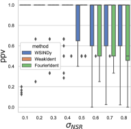
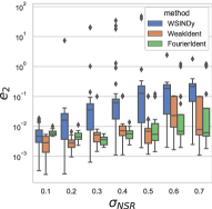
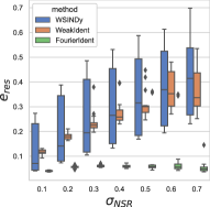
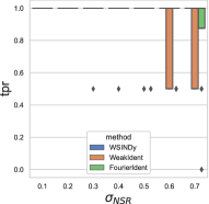
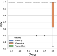
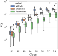
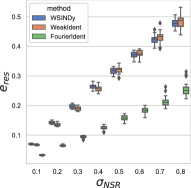
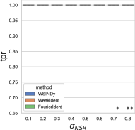
To measure the accuracy of identification, we use four identification errors in Table 1. They are the Relative coefficient error e2subscript𝑒2e_{2}, Relative residual error eressubscript𝑒𝑟𝑒𝑠e_{res}, True Positive Rate (TPR), and Positive Predictive Value (PPV). Here e2subscript𝑒2e_{2} measures the accuracy of the coefficient identification compared to the true coefficient; eressubscript𝑒𝑟𝑒𝑠e_{res} shows the relative residual error of fitting the identified differential equation to the given data; TPR provides the percentage of how many true features are identified compared to the total count of the true features; PPV provides the percentage of the true features identified as a result among all the identified features.

Name Definition Name Definition
e2subscript𝑒2e_{2} 𝒄𝒄true2𝒄2subscriptnorm𝒄subscript𝒄true2subscriptnorm𝒄2\frac{\|\boldsymbol{c}-\boldsymbol{c}_{\rm true}\|_{2}}{\|\boldsymbol{c}\|_{2}} TPR |{l:cpred(l)0,ctrue(l)0}||{l:ctrue(l)0|\frac{|\{l:c_{\rm pred}(l)\neq 0,c_{\rm true}(l)\neq 0\}|}{|\{l:c_{\rm true}(l)\neq 0|}
eressubscript𝑒rese_{\rm res} 𝑭𝒄𝒃2𝒃2subscriptnorm𝑭𝒄𝒃2subscriptnorm𝒃2\frac{\|\boldsymbol{F}\boldsymbol{c}-\boldsymbol{b}\|_{2}}{\|\boldsymbol{b}\|_{2}} PPV |{l:cpred(l)0,ctrue(l)0}||{l:cpred(l)0|\frac{|\{l:c_{\rm pred}(l)\neq 0,c_{\rm true}(l)\neq 0\}|}{|\{l:c_{\rm pred}(l)\neq 0|}
Table 1: We use four errors to measure the accuracy of identifying a partial differential equation in this paper: Relative coefficient error (e2subscript𝑒2e_{2}), Relative residual error (eressubscript𝑒rese_{\rm res}), True Positive Rate (TPR), and Positive Predictive Value (PPV).

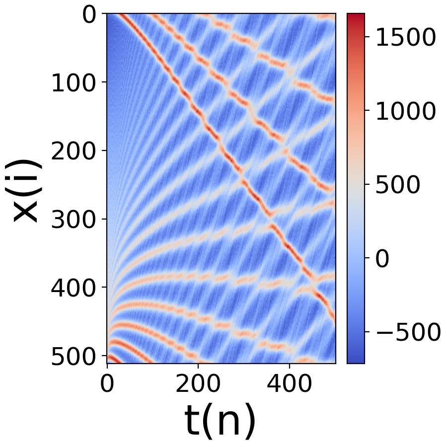
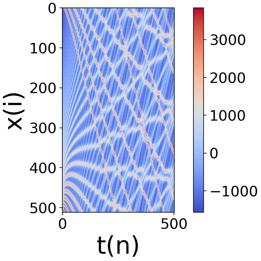
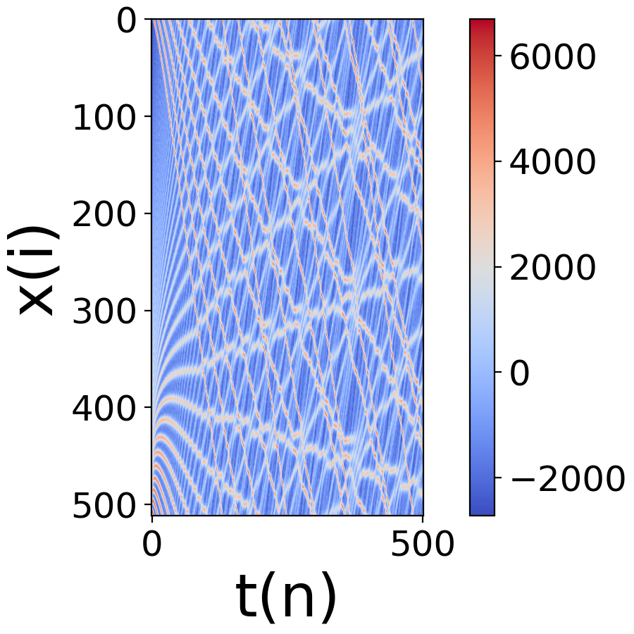
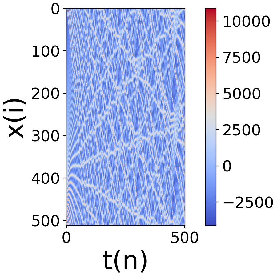
We experiment on various differential equations listed in Table 2. The Heat equation (35), Transport equation (36), and Burgers’ equation (37) are simulated using the spectrum method. The KdV (38) and KS (39) equation are simulated using the ETD RK4 method [20]. The true features in these equations contains ux,(u2)x,uxx,uxxx,subscript𝑢𝑥subscriptsuperscript𝑢2𝑥subscript𝑢𝑥𝑥subscript𝑢𝑥𝑥𝑥u_{x},(u^{2})_{x},u_{xx},u_{xxx}, and uxxxxsubscript𝑢𝑥𝑥𝑥𝑥u_{xxxx}. A diffusion term is added to the transport and burger equation to stabilize the pattern and increase the complexity of the model. These experiments show the robustness of FourierIdent in identifying linear, nonlinear, or higher-order derivative features.

Name Definition Simulation paramters
Heat Equation ut=0.12ux2𝑢𝑡0.1superscript2𝑢superscript𝑥2\frac{\partial u}{\partial t}=0.1\frac{\partial^{2}u}{\partial x^{2}} (35) T=[0,0.0999]𝑇00.0999T=[0,0.0999], [X1,X2]=[0,10]subscript𝑋1subscript𝑋2010[X_{1},X_{2}]=[0,10], Δx=0.0391Δ𝑥0.0391\Delta x=0.0391, Δt=0.003Δ𝑡0.003\Delta t=0.003.
Transport Equation with diffusion ut=ux+0.12ux2𝑢𝑡𝑢𝑥0.1superscript2𝑢superscript𝑥2\frac{\partial u}{\partial t}=-\frac{\partial u}{\partial x}+0.1\frac{\partial^{2}u}{\partial x^{2}} (36) T=[0,0.0999]𝑇00.0999T=[0,0.0999], [X1,X2]=[0,10]subscript𝑋1subscript𝑋2010[X_{1},X_{2}]=[0,10], Δx=0.0391Δ𝑥0.0391\Delta x=0.0391, Δt=0.003Δ𝑡0.003\Delta t=0.003.
Burger’s Equation with diffusion ut=0.25xu2+0.052ux2𝑢𝑡0.25𝑥superscript𝑢20.05superscript2𝑢superscript𝑥2\frac{\partial u}{\partial t}=0.25\frac{\partial}{\partial x}u^{2}+0.05\frac{\partial^{2}u}{\partial x^{2}} (37) T=[0,0.4995]𝑇00.4995T=[0,0.4995], [X1,X2]=[3.1416,3.1293]subscript𝑋1subscript𝑋23.14163.1293[X_{1},X_{2}]=[-3.1416,3.1293], Δx=0.0123Δ𝑥0.0123\Delta x=0.0123, Δt=0.001Δ𝑡0.001\Delta t=0.001.
Korteweg-de Vires (KdV) equation ut=0.5xu23ux3𝑢𝑡0.5𝑥superscript𝑢2superscript3𝑢superscript𝑥3\frac{\partial u}{\partial t}=-0.5\frac{\partial}{\partial x}u^{2}-\frac{\partial^{3}u}{\partial x^{3}} (38) T=[0,0.0200]𝑇00.0200T=[0,0.0200], [X1,X2]=[3.1416,3.1416]subscript𝑋1subscript𝑋23.14163.1416[X_{1},X_{2}]=[-3.1416,3.1416], Δx=0.0157Δ𝑥0.0157\Delta x=0.0157, Δt=4×10⁵Δ𝑡4superscript105\Delta t=4\times 10^{-5}.
Kuramoto-Sivashinsky (KS) ut=0.5xu22ux24ux4𝑢𝑡0.5𝑥superscript𝑢2superscript2𝑢superscript𝑥2superscript4𝑢superscript𝑥4\frac{\partial u}{\partial t}=-0.5\frac{\partial}{\partial x}u^{2}-\frac{\partial^{2}u}{\partial x^{2}}-\frac{\partial^{4}u}{\partial x^{4}} (39) T=[0,150]𝑇0150T=[0,150], [X1,X2]=[0,100.53]subscript𝑋1subscript𝑋20100.53[X_{1},X_{2}]=[0,100.53], Δx=0.3927Δ𝑥0.3927\Delta x=0.3927, Δt=0.5Δ𝑡0.5\Delta t=0.5.
Table 2: A list of equations used for experiments of FourierIdent. For all the equations, we use the maximum power β=6𝛽6\beta=6, maximum order of derivative α=6𝛼6\alpha=6, and total number of features L=43𝐿43L=43 as the dictionary’s parameters.

6.1 Workflow of FourierIdent

We illustrate the procedure of FourierIdent step by step, from constructing a feature matrix to achieving the identified coefficients.

In [Step 1], we obtain the feature matrix (18) and determine the core regions of features. Figure 3 shows an example of the KdV equation (38) with σNSR=0.3subscript𝜎NSR0.3\sigma_{\rm NSR}=0.3 noise. (a) shows the meaningful data region ΛΛ\Lambda (red box) in relation to the entire frequency domain, (b) shows the frequency response of uxxxsubscript𝑢𝑥𝑥𝑥u_{xxx} in ΛΛ\Lambda (zoomed), and (c) shows the core region of uxxxsubscript𝑢𝑥𝑥𝑥u_{xxx} restricted in ΛΛ\Lambda. Note the significant reduction of the size contributes to the efficiency of the method in (19).

(a) Frequency domain (b) (uxxx)subscript𝑢𝑥𝑥𝑥\mathcal{F}(u_{xxx}) on ΛΛ\Lambda (c) 𝒱(uxxx)𝒱subscript𝑢𝑥𝑥𝑥\mathcal{V}(u_{xxx})
Refer to caption Refer to caption Refer to caption
Figure 3: The KdV equation (38) with σNSR=0.3subscript𝜎𝑁𝑆𝑅0.3\sigma_{NSR}=0.3 as an example. (a) The frequency domain and ΛΛ\Lambda (the red box). (b) Zoom of ΛΛ\Lambda and the frequency response (|(uxxx)|)subscript𝑢𝑥𝑥𝑥\mathcal{R}(|\mathcal{F}(u_{xxx})|). (c) The white region represents the core region of uxxxsubscript𝑢𝑥𝑥𝑥u_{xxx} further reduced from ΛΛ\Lambda. There is a big reduction in the size of the region.

In [Step 2], for each sparsity level k=1,,K𝑘1𝐾k=1,\dots,K, we use Subspace Pursuit to obtain an initial candidate support 𝒜k0superscriptsubscript𝒜𝑘0\mathcal{A}_{k}^{0} which may be further reduced to a smaller support through group trimming. Table 3 shows the first result of SP, 𝒜k0subscriptsuperscript𝒜0𝑘\mathcal{A}^{0}_{k}, and how group trimming is iteratively applied to get 𝒜ksubscript𝒜𝑘\mathcal{A}_{k} for the KS equation (39). We present the cases for k5𝑘5k\leq 5, but we computed 𝒜ksubscript𝒜𝑘\mathcal{A}_{k} until k=10𝑘10k=10. When k=1𝑘1k=1, the candidate support has one feature (u2)xxxxsubscriptsuperscript𝑢2𝑥𝑥𝑥𝑥(u^{2})_{xxxx}, and the associated energy (25) is 0.8071. When k=3𝑘3k=3, the correct support is found as the initial support 𝒜30superscriptsubscript𝒜30\mathcal{A}_{3}^{0}, and no more feature is trimmed such that 𝒜3=𝒜30subscript𝒜3superscriptsubscript𝒜30\mathcal{A}_{3}=\mathcal{A}_{3}^{0}. When k=4𝑘4k=4, the feature (u4)xxxxsubscriptsuperscript𝑢4𝑥𝑥𝑥𝑥(u^{4})_{xxxx} is removed during group trimming. When k=5𝑘5k=5, the feature (u4)xxxx,(u2)xxxsubscriptsuperscript𝑢4𝑥𝑥𝑥𝑥subscriptsuperscript𝑢2𝑥𝑥𝑥(u^{4})_{xxxx},(u^{2})_{xxx} are removed during group trimming. The same support was obtained after group trimming when 3<k103𝑘103<k\leq 10. In the end, optimal ksuperscript𝑘k^{*} is given from 3, and the associated support is chosen to be 𝒜={uxx,uxxxx,(u2)x}superscript𝒜subscript𝑢𝑥𝑥subscript𝑢𝑥𝑥𝑥𝑥subscriptsuperscript𝑢2𝑥\mathcal{A}^{*}=\{u_{xx},u_{xxxx},(u^{2})_{x}\}.

Sparsity Support ksuperscript𝑘k^{*} energy (25)
SP(1) 𝒜10={(u2)xxxx}=𝒜1superscriptsubscript𝒜10subscriptsuperscript𝑢2𝑥𝑥𝑥𝑥subscript𝒜1\mathcal{A}_{1}^{0}=\{(u^{2})_{xxxx}\}=\mathcal{A}_{1} 0.8071
SP(2) 𝒜20={(u2)xxxx,(u2)xx}=𝒜2superscriptsubscript𝒜20subscriptsuperscript𝑢2𝑥𝑥𝑥𝑥subscriptsuperscript𝑢2𝑥𝑥subscript𝒜2\mathcal{A}_{2}^{0}=\{(u^{2})_{xxxx},(u^{2})_{xx}\}=\mathcal{A}_{2} 4.1957
SP(3) 𝒜30={uxx,uxxxx,(u2)x}=𝒜3superscriptsubscript𝒜30subscript𝑢𝑥𝑥subscript𝑢𝑥𝑥𝑥𝑥subscriptsuperscript𝑢2𝑥subscript𝒜3\mathcal{A}_{3}^{0}=\{u_{xx},u_{xxxx},(u^{2})_{x}\}=\mathcal{A}_{3} 0.1975
SP(4) 𝒜40={uxx,uxxxx,(u2)x,(u4)xxxx}superscriptsubscript𝒜40subscript𝑢𝑥𝑥subscript𝑢𝑥𝑥𝑥𝑥subscriptsuperscript𝑢2𝑥subscriptsuperscript𝑢4𝑥𝑥𝑥𝑥\mathcal{A}_{4}^{0}=\{u_{xx},u_{xxxx},(u^{2})_{x},(u^{4})_{xxxx}\}
            Score (20) s(uxx)=1,s(uxxxx)=0.59,s((u2)x)=0.63formulae-sequence𝑠subscript𝑢𝑥𝑥1formulae-sequence𝑠subscript𝑢𝑥𝑥𝑥𝑥0.59𝑠subscriptsuperscript𝑢2𝑥0.63s(u_{xx})=1,s(u_{xxxx})=0.59,s((u^{2})_{x})=0.63, s((u4)xxxx)=0.01𝑠subscriptsuperscript𝑢4𝑥𝑥𝑥𝑥0.01s((u^{4})_{xxxx})=0.01
            Updated 𝒜41={uxx,uxxxx,(u2)x}=𝒜4superscriptsubscript𝒜41subscript𝑢𝑥𝑥subscript𝑢𝑥𝑥𝑥𝑥subscriptsuperscript𝑢2𝑥subscript𝒜4\mathcal{A}_{4}^{1}=\{u_{xx},u_{xxxx},(u^{2})_{x}\}=\mathcal{A}_{4} 0.1975
SP(5) 𝒜50={uxx,uxxxx,(u2)x(u2)xxx,(u4)xxxx}superscriptsubscript𝒜50subscript𝑢𝑥𝑥subscript𝑢𝑥𝑥𝑥𝑥subscriptsuperscript𝑢2𝑥subscriptsuperscript𝑢2𝑥𝑥𝑥subscriptsuperscript𝑢4𝑥𝑥𝑥𝑥\mathcal{A}_{5}^{0}=\{u_{xx},u_{xxxx},(u^{2})_{x}(u^{2})_{xxx},(u^{4})_{xxxx}\}
            Score (20) s(uxx)=1,s(uxxxx)=0.59,s((u2)x)=0.65formulae-sequence𝑠subscript𝑢𝑥𝑥1formulae-sequence𝑠subscript𝑢𝑥𝑥𝑥𝑥0.59𝑠subscriptsuperscript𝑢2𝑥0.65s(u_{xx})=1,s(u_{xxxx})=0.59,s((u^{2})_{x})=0.65,
s((u4)xxxx)=0.04,s((u2)x)=0.02formulae-sequence𝑠subscriptsuperscript𝑢4𝑥𝑥𝑥𝑥0.04𝑠subscriptsuperscript𝑢2𝑥0.02s((u^{4})_{xxxx})=0.04,s((u^{2})_{x})=0.02
            Updated 𝒜51={uxx,uxxxx,(u2)x}=𝒜5superscriptsubscript𝒜51subscript𝑢𝑥𝑥subscript𝑢𝑥𝑥𝑥𝑥subscriptsuperscript𝑢2𝑥subscript𝒜5\mathcal{A}_{5}^{1}=\{u_{xx},u_{xxxx},(u^{2})_{x}\}=\mathcal{A}_{5} 0.1975
Table 3: The KS equation in (39) with σNSR=0.5subscript𝜎NSR0.5\sigma_{\rm NSR}=0.5 as an example. [Step 2] SP and group trimming. For each sparsity level k𝑘k, SP(k𝑘k) represents Subspace Pursuit applied on 𝒮(𝑭)𝒱(ut)𝒮superscriptsubscript𝑭𝒱subscript𝑢𝑡{\mathcal{S}(\boldsymbol{F})_{\mathcal{V}(u_{t})}}^{\dagger}, we show the initial support and the converged support 𝒜ksubscript𝒜𝑘\mathcal{A}_{k} after the group trimming. While no features are trimmed when k3𝑘3k\leq 3, for k>3𝑘3k>3 with the group trimming, it converged in one step. Note the same features 𝒜superscript𝒜\mathcal{A}^{*} are found from k=3𝑘3k=3 with the minimum energy (25).

In [Step 3], we pick the coefficient vector with the minimum energy based on the core region of features (25). Note that these coefficient energies are associated with each individual core region, and Table 4 presents this computation from the features of 𝒜superscript𝒜\mathcal{A}^{*} and utsubscript𝑢𝑡u_{t}, i.e., 𝒱(ut),𝒱(uxx),𝒱(uxxxx),𝒱((u2)x)𝒱subscript𝑢𝑡𝒱subscript𝑢𝑥𝑥𝒱subscript𝑢𝑥𝑥𝑥𝑥𝒱subscriptsuperscript𝑢2𝑥\mathcal{V}(u_{t}),\mathcal{V}(u_{xx}),\mathcal{V}(u_{xxxx}),\mathcal{V}((u^{2})_{x}), for the KS equation (39). The coefficient values are similar to each other, thanks to the consistency term (24) in (25), and we choose the best coefficient vector. In this example, 𝒱=𝒱(uxxxx)superscript𝒱𝒱subscript𝑢𝑥𝑥𝑥𝑥\mathcal{V}^{*}=\mathcal{V}(u_{xxxx}) gives the lowest coefficient energy. The final output of this identification example is ut=0.9701uxx0.9916uxxxx0.4785(u2)xsubscript𝑢𝑡0.9701subscript𝑢𝑥𝑥0.9916subscript𝑢𝑥𝑥𝑥𝑥0.4785subscriptsuperscript𝑢2𝑥u_{t}=-0.9701u_{xx}-0.9916u_{xxxx}-0.4785(u^{2})_{x} and the true equation is ut=uxxuxxxx0.5(u2)xsubscript𝑢𝑡subscript𝑢𝑥𝑥subscript𝑢𝑥𝑥𝑥𝑥0.5subscriptsuperscript𝑢2𝑥u_{t}=-u_{xx}-u_{xxxx}-0.5(u^{2})_{x} in (39).

Features in 𝒜ksuperscriptsubscript𝒜𝑘\mathcal{A}_{k}^{*} Coefficients Residual error (26)
Use 𝒮(𝑭)𝒱(ut)𝒮subscript𝑭𝒱subscript𝑢𝑡\mathcal{S}(\boldsymbol{F})_{\mathcal{V}(u_{t})} 𝒄𝒱(ut)=[0.8834,0.881,0.4443]subscript𝒄𝒱subscript𝑢𝑡0.88340.8810.4443\boldsymbol{c}_{\mathcal{V}(u_{t})}=[-0.8834,-0.881,-0.4443] 0.2817
Use 𝒮(𝑭)𝒱(uxx)𝒮subscript𝑭𝒱subscript𝑢𝑥𝑥\mathcal{S}(\boldsymbol{F})_{\mathcal{V}(u_{xx})} 𝒄𝒱(uxx)=[0.8912,0.8921,0.4464]subscript𝒄𝒱subscript𝑢𝑥𝑥0.89120.89210.4464\boldsymbol{c}_{\mathcal{V}(u_{xx})}=[-0.8912,-0.8921,-0.4464] 0.2817
Use 𝒮(𝑭)𝒱(uxxxx)𝒮subscript𝑭𝒱subscript𝑢𝑥𝑥𝑥𝑥\mathcal{S}(\boldsymbol{F})_{\mathcal{V}(u_{xxxx})} 𝒄𝒱(uxxxx)=[0.9701,0.9916,0.4785]subscript𝒄𝒱subscript𝑢𝑥𝑥𝑥𝑥0.97010.99160.4785\boldsymbol{c}_{\mathcal{V}(u_{xxxx})}=[-0.9701,-0.9916,-0.4785] 0.1468
Use 𝒮(𝑭)𝒱((u2)x)𝒮subscript𝑭𝒱subscriptsuperscript𝑢2𝑥\mathcal{S}(\boldsymbol{F})_{\mathcal{V}((u^{2})_{x})} 𝒄𝒱((u2)x)=[0.9642,0.9706,0.4867]subscript𝒄𝒱subscriptsuperscript𝑢2𝑥0.96420.97060.4867\boldsymbol{c}_{\mathcal{V}((u^{2})_{x})}=[-0.9642,-0.9706,-0.4867] 0.1483
Identified equation becomes ut=0.9701uxx0.9916uxxxx0.4785(u2)xsubscript𝑢𝑡0.9701subscript𝑢𝑥𝑥0.9916subscript𝑢𝑥𝑥𝑥𝑥0.4785subscriptsuperscript𝑢2𝑥u_{t}=-0.9701u_{xx}-0.9916u_{xxxx}-0.4785(u^{2})_{x}, using 𝒱=𝒱(uxxxx)superscript𝒱𝒱subscript𝑢𝑥𝑥𝑥𝑥\mathcal{V}^{*}=\mathcal{V}(u_{xxxx}),
Table 4: The KS equation in (39) with σNSR=0.5subscript𝜎NSR0.5\sigma_{\rm NSR}=0.5. [Step 3] for each features of 𝒜{ut}={ut,uxx,uxxxx,(u2)x}superscript𝒜subscript𝑢𝑡subscript𝑢𝑡subscript𝑢𝑥𝑥subscript𝑢𝑥𝑥𝑥𝑥subscriptsuperscript𝑢2𝑥\mathcal{A}^{*}\cup\{u_{t}\}=\{u_{t},u_{xx},u_{xxxx},(u^{2})_{x}\} computes the coefficients and find the minimum residual energy (26) feature. The minimum coefficient energy is given by 𝒱=𝒱(uxxxx)superscript𝒱𝒱subscript𝑢𝑥𝑥𝑥𝑥\mathcal{V}^{*}=\mathcal{V}(u_{xxxx}) and the corresponding equation is identified.

6.2 Effect of the meaningful data region ΛΛ\Lambda

We present the effect of the meaningful data region, using the KdV equation with σNSR=0.3subscript𝜎NSR0.3\sigma_{\rm NSR}=0.3 as an example. Figure 4 shows the scale of features of 𝑭𝑭\boldsymbol{F}, 𝑭Λsubscript𝑭Λ\boldsymbol{F}_{\Lambda} (𝑭𝑭\boldsymbol{F} restricted on ΛΛ\Lambda), 𝒮(𝑭)𝒮𝑭\mathcal{S}(\boldsymbol{F}), 𝒮(𝑭)Λ𝒮subscript𝑭Λ\mathcal{S}(\boldsymbol{F})_{\Lambda} and 𝑾𝑾\boldsymbol{W} which is the Weak-form feature in the physical domain as in WeakIdent [30]. The magnitude of the Fourier features have a wider range, and using the meaningful data region ΛΛ\Lambda helps to reduce this range by comparing 𝑭𝑭\boldsymbol{F} with 𝑭Λsubscript𝑭Λ\boldsymbol{F}_{\Lambda} and 𝒮(𝑭)𝒮𝑭\mathcal{S}(\boldsymbol{F}) with 𝒮(𝑭)Λ𝒮subscript𝑭Λ\mathcal{S}(\boldsymbol{F})_{\Lambda}. With ΛΛ\Lambda restriction, the shape of the graph looks similar to the physical values of Weak form. In addition, due to the symmetry, a quarter of data is used, i.e., the frequencies ξx,ξtsubscript𝜉𝑥subscript𝜉𝑡\xi_{x},\xi_{t} with the same magnitude have similar behaviors. We take a smaller collection of the frequency modes which reduces the computational cost.
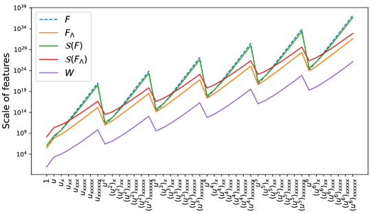
Refer to caption
Figure 4: Effect of the meaningful data region ΛΛ\Lambda, illustrated by the KdV equation (38) with σNSR=0.3subscript𝜎NSR0.3\sigma_{\rm NSR}=0.3. The x-axis provides a list of features and the y-axis represents the scale of features in terms of the 2subscript2\ell_{2}-norm of the feature column. We compare 𝑭𝑭\boldsymbol{F} with 𝑭Λsubscript𝑭Λ\boldsymbol{F}_{\Lambda}, 𝒮(𝑭)𝒮𝑭\mathcal{S}(\boldsymbol{F}) with 𝒮(𝑭)Λ𝒮subscript𝑭Λ\mathcal{S}(\boldsymbol{F})_{\Lambda}, and Fourier features with the Weak-form features in 𝑾𝑾\boldsymbol{W} in WeakIdent [30]. A restriction to the meaningful data region ΛΛ\Lambda helps to reduce the range of Fourier features and make the shape of the scale similar to that in the weak form.

In Table 5, we compare the identification results with or without the restriction to the meaningful data region ΛΛ\Lambda. For the KdV equation (38) and the KS equation (39) on clean and noise data σNSR=0.3subscript𝜎NSR0.3\sigma_{\rm NSR}=0.3, we show how the restriction to ΛΛ\Lambda helps to find the correct equation. Without noise, the restriction to ΛΛ\Lambda makes little differences. When the noise level increases, the results without restriction to ΛΛ\Lambda may give completely wrong results.

KdV Eq. (38) true equation ut=1.0uxxx0.5(u2)xsubscript𝑢𝑡1.0subscript𝑢𝑥𝑥𝑥0.5subscriptsuperscript𝑢2𝑥u_{t}=-1.0u_{xxx}-0.5(u^{2})_{x}
σNSR=0subscript𝜎NSR0\sigma_{\rm NSR}=0 with ΛΛ\Lambda ut=0.998uxxx0.499(u2)xsubscript𝑢𝑡0.998subscript𝑢𝑥𝑥𝑥0.499subscriptsuperscript𝑢2𝑥u_{t}=-0.998u_{xxx}-0.499(u^{2})_{x}
without ΛΛ\Lambda ut=0.998uxxx0.499(u2)xsubscript𝑢𝑡0.998subscript𝑢𝑥𝑥𝑥0.499subscriptsuperscript𝑢2𝑥u_{t}=-0.998u_{xxx}-0.499(u^{2})_{x}
σNSR=0.3subscript𝜎NSR0.3\sigma_{\rm NSR}=0.3 with ΛΛ\Lambda ut=1.012uxxx0.499(u2)xsubscript𝑢𝑡1.012subscript𝑢𝑥𝑥𝑥0.499subscriptsuperscript𝑢2𝑥u_{t}=-1.012u_{xxx}-0.499(u^{2})_{x}
without ΛΛ\Lambda ut=151.987uxsubscript𝑢𝑡151.987subscript𝑢𝑥u_{t}=-151.987u_{x}
KS Eq. (39) true equation ut=1.0uxx1.0uxxxx0.5(u2)xsubscript𝑢𝑡1.0subscript𝑢𝑥𝑥1.0subscript𝑢𝑥𝑥𝑥𝑥0.5subscriptsuperscript𝑢2𝑥u_{t}=-1.0u_{xx}-1.0u_{xxxx}-0.5(u^{2})_{x}
σNSR=0subscript𝜎NSR0\sigma_{\rm NSR}=0 with ΛΛ\Lambda ut=1.0uxx1.0uxxxx0.5(u2)xsubscript𝑢𝑡1.0subscript𝑢𝑥𝑥1.0subscript𝑢𝑥𝑥𝑥𝑥0.5subscriptsuperscript𝑢2𝑥u_{t}=-1.0u_{xx}-1.0u_{xxxx}-0.5(u^{2})_{x}
without ΛΛ\Lambda ut=0.999uxx0.999uxxxx0.5(u2)xsubscript𝑢𝑡0.999subscript𝑢𝑥𝑥0.999subscript𝑢𝑥𝑥𝑥𝑥0.5subscriptsuperscript𝑢2𝑥u_{t}=-0.999u_{xx}-0.999u_{xxxx}-0.5(u^{2})_{x}
σNSR=0.3subscript𝜎NSR0.3\sigma_{\rm NSR}=0.3 with ΛΛ\Lambda ut=0.978uxx0.977uxxxx0.49(u2)xsubscript𝑢𝑡0.978subscript𝑢𝑥𝑥0.977subscript𝑢𝑥𝑥𝑥𝑥0.49subscriptsuperscript𝑢2𝑥u_{t}=-0.978u_{xx}-0.977u_{xxxx}-0.49(u^{2})_{x}
without ΛΛ\Lambda ut=0.035(u4)xsubscript𝑢𝑡0.035subscriptsuperscript𝑢4𝑥u_{t}=-0.035(u^{4})_{x}
Table 5: Effect of applying FourierIdent with or without restriction to the meaningful data region ΛΛ\Lambda. With an increased level of noise, the benefit of having ΛΛ\Lambda is clearly demonstrated.
(a) σNSR=0.8subscript𝜎NSR0.8\sigma_{\rm NSR}=0.8 (b) σNSR=0.8subscript𝜎NSR0.8\sigma_{\rm NSR}=0.8
Refer to caption Refer to caption
Figure 5: Benefits of using the energy in (25) to find the optimal ksuperscript𝑘k^{*}. (a) and (b) are both for KS equation with σNSR=0.8subscript𝜎NSR0.8\sigma_{\rm NSR}=0.8. The x-axis represents the initial sparsity level. The dots represent the cases when the trimmed support is the correct one. In (a), the y-axis represents the values of Cross-Validation error and the energy in (25). When the given data are noisy, as in (a), the results with sparsity levels 10,13,14,151013141510,13,14,15 give rise to small cross-validation errors but large energy 1+2subscript1subscript2\mathcal{E}_{1}+\mathcal{E}_{2} defined in (25). In (b), the green curve shows the fitting residual 1subscript1\mathcal{E}_{1} in (23), and the purple curve shows the stability term 2subscript2\mathcal{E}_{2} in (24). The new energy as the sum of the fitting residual and the stability term is represented by the yellow curve.

6.3 Understanding the new energy in (25)

We introduce a new energy based on the core regions of features in Section 4.2. In this subsection, we show the effect of the energy in (25) compared to the Cross-Validation (CV) error used in [13, 30]. In Figure 5, we present the result for the KS equation (39) with σNSR=0.8subscript𝜎NSR0.8\sigma_{\rm NSR}=0.8. In Figure 5 (a), the yellow curve shows the new energy (25) value and the blue curve shows the CV error. The x-axis shows the initial sparsity as the input of SP, and the sparsity after group trimming is usually much smaller than the initial sparsity. The yellow and blue circles indicate the cases when the correct supports are found after group trimming. After the sparsity level k=3𝑘3k=3, the CV errors are all similarly low. If we use the CV error, the wrong supports are identified when k=10,13,14,15𝑘10131415k=10,13,14,15. The yellow curve using the new energy is more consistent: the sparsity associated with a low energy corresponds to the correct support. Figure 5 (b) shows the values of the two terms in the energy (25): the green curve shows the fitting residual 1subscript1\mathcal{E}_{1}, and the purple curve shows the stability term 2subscript2\mathcal{E}_{2}. The yellow curve shows the sum of them, which is the same as the yellow curve in Figure 5 (a). While the residual curve (green curve) is minimized at the wrong sparsity k=1𝑘1k=1, the total energy as the sum of the fitting residual and the stability term is minimized at the correct sparsity and support.

6.4 FourierIdent experiments with an increasing complexity

We experiment FourierIdent with an increasing complexity of the initial conditions. We use the KdV equation in (38) with different initial conditions (IC) where we can control the complexity:

u0=r=1Rcos(rx+c1)+sin(rx+c2),subscript𝑢0superscriptsubscript𝑟1𝑅𝑟𝑥subscript𝑐1𝑟𝑥subscript𝑐2u_{0}=\sum_{r=1}^{R}\cos(rx+c_{1})+\sin(rx+c_{2}), (40)

where c1subscript𝑐1c_{1} and c2subscript𝑐2c_{2} are two random numbers and R𝑅R denotes the total number of modes used in u0subscript𝑢0u_{0}. The larger the R𝑅R is, the more complex the given data are in both physical and frequency domains. We use periodic spatial domain such that x[3.1416,3.1293]𝑥3.14163.1293x\in[-3.1416,3.1293] with spatial spacing Δx=0.123Δ𝑥0.123\Delta x=0.123 and the time domain t[0,0.02]𝑡00.02t\in[0,0.02] with temporal spacing Δt=3.9978×10⁵Δ𝑡3.9978superscript105\Delta t=3.9978\times 10^{-5}. In Figure 6 (a) - (e), we show clean data for the initial conditions with R=𝑅absentR= 1, 20, 30, 40, and 50 modes. It is shown that the pattern in (a) is relatively simple, and pattern in (e) is the most complex one. We use a simulated solution from each complexity mode from R=1𝑅1R=1 to R=60𝑅60R=60.

(a) 1 mode (b) 20 modes (c) 30 modes (d) 40 modes (e) 50 modes
Refer to caption Refer to caption Refer to caption Refer to caption Refer to caption
(f) σNSR=0.2subscript𝜎NSR0.2\sigma_{\rm NSR}=0.2 (g) σNSR=0.25subscript𝜎NSR0.25\sigma_{\rm NSR}=0.25 (h) σNSR=0.3subscript𝜎NSR0.3\sigma_{\rm NSR}=0.3 (i) σNSR=0.35subscript𝜎NSR0.35\sigma_{\rm NSR}=0.35
Refer to caption Refer to caption Refer to caption Refer to caption
Figure 6: Influence of increasing complexity. (a) - (e) Clean data of the KdV equation (38) for the initial condition (40) with R=𝑅absentR= 1, 20, 30, 40, and 50. From (a) to (e), the patterns become more complex. (f) - (i) show comparison results between FourierIdeant and WeakIdent for different noise levels such that σNSR{0.05,0.1,0.15,0.2,0.25,0.3,0.35}subscript𝜎NSR0.050.10.150.20.250.30.35\sigma_{\rm NSR}\in\{0.05,0.1,0.15,0.2,0.25,0.3,0.35\}. Each dot represents the e2subscript𝑒2e_{2} identification error in each experiment. When 10<R<4010𝑅4010<R<40, FourierIdent gives rise to more accurate recovery results.

Figure 6 (f)-(i) show the performance of FourierIdent compared with WeakIdent, for different level of noise such that σNSR=0.2,0.25,0.3,0.35subscript𝜎NSR0.20.250.30.35\sigma_{\rm NSR}=0.2,0.25,0.3,0.35. For each mode R𝑅R ranging from 1 to 60, we simulate 20 different datasets with different random seeds. In each graph, each column contains 20 dots for the 20 independent experiments, and the height represents the e2subscript𝑒2e_{2} identification error of Fourierident (blue) and WeakIdent (yellow).

This experiment shows that, for data with different complexity and with different noise levels, FourierIdent gives rise to smaller e2subscript𝑒2e_{2} errors. Figures (f)-(i) shows that when K>10𝐾10K>10, FourierIdent (marked in blue) performs better than WeakIdent (marked in yellow), when σNSRsubscript𝜎𝑁𝑆𝑅\sigma_{NSR} is large and the data have more frequency modes.

6.5 FourierIdent experiment with an increasing time for data collection

The next experiment shows how the increasing of time interval for data collection can improve the identification result. Figure 7 (a) and (b) show a realization of the given data for the KS equation (39) with σNSR=0.5subscript𝜎NSR0.5\sigma_{\rm NSR}=0.5. (a) is for 0<t<5000𝑡5000<t<500 and (b) is for 0<t<5,000formulae-sequence0𝑡50000<t<5,000. The data in (b) clearly have more repetition of the pattern. Figure 7 (c)-(e) show experiments with varying noise levels such that σNSR=0.01,0.5,1.0subscript𝜎NSR0.010.51.0\sigma_{\rm NSR}=0.01,0.5,1.0. For each graph, the x-axis represents the final time tendsubscript𝑡𝑒𝑛𝑑t_{end} used for the data, and y-axis shows the e2subscript𝑒2e_{2} error of the identified coefficient. In (c), when the noise level is low, both FourierIdent and WeakIdent show good results with the e2subscript𝑒2e_{2} error less than 103superscript10310^{-3}. This is based on one experiment for each noise level. As the noise level increases, FourierIdent consistently gives better results in (d) and (e). (e) shows an extremely noisy case for σNSR=1subscript𝜎NSR1\sigma_{\rm NSR}=1 when the given data are highly corrupted by noise. For both (d) and (e), as tendsubscript𝑡𝑒𝑛𝑑t_{end} gets bigger, both FourierIdent and WeakIdent give rise to decreasing errors , and the error of FourierIdent is lower. The core region is defined by the high frequency responses, thus with more data, the response will be stronger and the core region of feature can separate the noise better. FourierIdent is slightly worse than WeakIdent when σSNR=0.01subscript𝜎SNR0.01\sigma_{\rm SNR}=0.01 compared to σSNR=0.5subscript𝜎SNR0.5\sigma_{\rm SNR}=0.5 or 1.0. This shows the effect that FourierIent performs well due to having enough high-frequency responses when the data are exposed to large noise. In other words, FourierIdent is relatively more effective and robust under noise compared to methods using physical features, which is consistent with our observation in Figure 6.

(a) 0t5000𝑡5000\leq t\leq 500 (b) 0t5,000formulae-sequence0𝑡50000\leq t\leq 5,000
Refer to caption Refer to caption
(c) σNSR=0.01subscript𝜎NSR0.01\sigma_{\rm NSR}=0.01 (d) σNSR=0.5subscript𝜎NSR0.5\sigma_{\rm NSR}=0.5 (e) σNSR=1.0subscript𝜎NSR1.0\sigma_{\rm NSR}=1.0
Refer to caption Refer to caption Refer to caption
Figure 7: Influence of increasing time in data collection. (a) - (b): The given data of the KS equation (39) (a) for 0<t<5000𝑡5000<t<500, and (b) for 0<t<5,000formulae-sequence0𝑡50000<t<5,000. (c)-(e): the x𝑥x-axis represents the final time tendsubscript𝑡𝑒𝑛𝑑t_{end} for data collection, and the y𝑦y-axis shows the e2subscript𝑒2e_{2} error of the identified coefficient, for FourierIdent (blue) and WeakIdent (yellow). In (c), for low levels of noise σNSR=0.01subscript𝜎NSR0.01\sigma_{\rm NSR}=0.01, both FourierIdent (blue) and WeakIdent (yellow) give small e2subscript𝑒2e_{2} errors. In (d) and (e), when σNSR=0.5subscript𝜎NSR0.5\sigma_{\rm NSR}=0.5 and 111, as tendsubscript𝑡𝑒𝑛𝑑t_{end} gets bigger, both FourierIdent and WeakIdent yield smaller errors, while FourierIdent gives rise to a smaller error than WeakIdent.

6.6 FourierIdent comparison results

We test FourierIdent, and compare it with WeakIdent[30] and WSINDy [21]. We first present an example showing the identified equations, and then present more statistics about the recovery. In Table 6, we present the identified equation and the e2subscript𝑒2e_{2} error for the equations listed in Table 2 with σNSR=0.3subscript𝜎NSR0.3\sigma_{\rm NSR}=0.3. FourierIdent identifies the correct equation, i.e., the correct support and highly accurate coefficient values, under various scenarios.

Equ σNSRsubscript𝜎NSR\sigma_{\rm NSR} Method Identified equation e2subscript𝑒2e_{2}
(35) 0.3 FourierIdent ut=+0.1uxxsubscript𝑢𝑡0.1subscript𝑢𝑥𝑥u_{t}=+0.1u_{xx} 0.002536
WeakIdent ut=+0.1uxxsubscript𝑢𝑡0.1subscript𝑢𝑥𝑥u_{t}=+0.1u_{xx} 0.003609
WSINDy ut=0.098uxxsubscript𝑢𝑡0.098subscript𝑢𝑥𝑥u_{t}=0.098u_{xx} 0.012311
(36) 0.3 FourierIdent ut=1.0ux+0.099uxxsubscript𝑢𝑡1.0subscript𝑢𝑥0.099subscript𝑢𝑥𝑥u_{t}=-1.0u_{x}+0.099u_{xx} 0.000719
WeakIdent ut=0.997ux+0.102uxxsubscript𝑢𝑡0.997subscript𝑢𝑥0.102subscript𝑢𝑥𝑥u_{t}=-0.997u_{x}+0.102u_{xx} 0.003477
WSINDy ut=0.434+0.793uxxxxxx1.003u2+0.096(u2)x+0.470(u2)xxxxxxu_{t}=0.434+-0.793u_{xxxxxx}-1.003u^{2}+0.096(u^{2})_{x}+0.470(u^{2})_{xxxxxx} 1.017465
(37) 0.3 FourierIdent ut=+0.051uxx+0.249(u2)xsubscript𝑢𝑡0.051subscript𝑢𝑥𝑥0.249subscriptsuperscript𝑢2𝑥u_{t}=+0.051u_{xx}+0.249(u^{2})_{x} 0.006846
WeakIdent ut=+0.052uxx+0.248(u2)xsubscript𝑢𝑡0.052subscript𝑢𝑥𝑥0.248subscriptsuperscript𝑢2𝑥u_{t}=+0.052u_{xx}+0.248(u^{2})_{x} 0.011226
WSINDy ut=+0.048uxx+0.248(u2)xsubscript𝑢𝑡0.048subscript𝑢𝑥𝑥0.248subscriptsuperscript𝑢2𝑥u_{t}=+0.048u_{xx}+0.248(u^{2})_{x} 0.009981
(38) 0.3 FourierIdent ut=0.997uxxx0.499(u2)xsubscript𝑢𝑡0.997subscript𝑢𝑥𝑥𝑥0.499subscriptsuperscript𝑢2𝑥u_{t}=-0.997u_{xxx}-0.499(u^{2})_{x} 0.0031048
WeakIdent ut=0.987uxxx0.497(u2)xsubscript𝑢𝑡0.987subscript𝑢𝑥𝑥𝑥0.497subscriptsuperscript𝑢2𝑥u_{t}=-0.987u_{xxx}-0.497(u^{2})_{x} 0.0121109
WSINDy ut=0.977uxxx0.4967(u2)xsubscript𝑢𝑡0.977subscript𝑢𝑥𝑥𝑥0.4967subscriptsuperscript𝑢2𝑥u_{t}=-0.977u_{xxx}-0.4967(u^{2})_{x} 0.0203434
(39) 0.3 FourierIdent ut=0.977uxx0.97uxxxx0.488(u2)xsubscript𝑢𝑡0.977subscript𝑢𝑥𝑥0.97subscript𝑢𝑥𝑥𝑥𝑥0.488subscriptsuperscript𝑢2𝑥u_{t}=-0.977u_{xx}-0.97u_{xxxx}-0.488(u^{2})_{x} 0.02663459
WeakIdent ut=0.95uxx0.947uxxxx0.476(u2)xsubscript𝑢𝑡0.95subscript𝑢𝑥𝑥0.947subscript𝑢𝑥𝑥𝑥𝑥0.476subscriptsuperscript𝑢2𝑥u_{t}=-0.95u_{xx}-0.947u_{xxxx}-0.476(u^{2})_{x} 0.051067
WSINDy ut=0.9529uxx0.9493uxxxx0.4779(u2)xu_{t}=-0.9529u_{xx}-0.9493u_{xxxx}--0.4779(u^{2})_{x} 0.048433
Table 6: Identification results by FourierIdent, WeakIdent[30] and WSINDy [21] for the equations in Table 2 with σNSR=0.3subscript𝜎NSR0.3\sigma_{\rm NSR}=0.3 using one realization of the PDE solution.

We further show the recovery statistics for the equations in Table 2, in Figure 8, 10, 9, 11, and 12. We present the results with different noise-to-signal-ratio σNSRsubscript𝜎NSR\sigma_{\rm NSR} using box plots of the identification error for FourierIdent, WeakIdent[30] and WSINDy [21]. For each σNSRsubscript𝜎NSR\sigma_{\rm NSR}, the dataset is simulated 20 times with various random seeds of noise. FourierIdent is compatible with other methods in identifying a partial differential equation. It is robust to high levels of noise and capable of dealing with features with high-order derivatives.

(a) (b) (c) (d)
Refer to caption Refer to caption Refer to caption Refer to caption
Figure 8: Heat equation (35). (a) e2subscript𝑒2e_{2} error, (b) eressubscript𝑒𝑟𝑒𝑠e_{res}, (c) TPR, and (d) PPV. For each noise level σNSRsubscript𝜎NSR\sigma_{\rm NSR}, we generate noise using 20 random seeds, and show a box plot for FourierIdent, WeakIdent, and WSINDy.
(a) (b) (c) (d)
Refer to caption Refer to caption Refer to caption Refer to caption
Figure 9: Transport equation (36). (a) e2subscript𝑒2e_{2} error, (b) eressubscript𝑒𝑟𝑒𝑠e_{res}, (c) TPR, and (d) PPV. For each noise level σNSRsubscript𝜎NSR\sigma_{\rm NSR}, we generate noise using 20 random seeds, and show a box plot for FourierIdent, WeakIdent, and WSINDy.
(a) (b) (c) (d)
Refer to caption Refer to caption Refer to caption Refer to caption
Figure 10: The Burgers’ equation (37). (a) e2subscript𝑒2e_{2} error, (b) eressubscript𝑒𝑟𝑒𝑠e_{res}, (c) TPR, and (d) PPV. For each noise level σNSRsubscript𝜎NSR\sigma_{\rm NSR}, we generate noise using 20 random seeds, and show a box plot for FourierIdent, WeakIdent, and WSINDy.
(a) (b) (c) (d)
Refer to caption Refer to caption Refer to caption Refer to caption
Figure 11: The KdV equation (38). (a) e2subscript𝑒2e_{2} error, (b) eressubscript𝑒𝑟𝑒𝑠e_{res}, (c) TPR, and (d) PPV. For each noise level σNSRsubscript𝜎𝑁𝑆𝑅\sigma_{NSR}, we generate noise using 20 random seeds, and show a box plot for FourierIdent, WeakIdent, and WSINDy.
(a) (b) (c) (d)
Refer to caption Refer to caption Refer to caption Refer to caption
Figure 12: Comparison results on the KS equation (39) using multiple identification errors e2subscript𝑒2e_{2} in (a), eressubscript𝑒𝑟𝑒𝑠e_{res} in (b), TPR in (c), and PPV in (d). For each noise level σNSRsubscript𝜎𝑁𝑆𝑅\sigma_{NSR}, we generate noise using 20 random seeds and show a box plot for FourierIdent, WeakIdent, and WSINDy.

7 Discussion and Conclusion

We proposed FourierIdent, a method to identify differential equations in the frequency domain. We introduced denoising Fourier features by smoothing, and frequency domain partitioning, e.g., the meaningful data region and the core regions of features. We proposed an energy based on the core regions of features for coefficient identification. Different collections of high frequency responses are used to identify features and improve coefficient recovery. We present numerical experiments on various simulated datasets to compare FourierIdent with other state-of-art methods using weak formulations. FourierIdent is robust to noise and can handle higher-order derivatives. We show the benefits of FourierIdent on complex datasets simulated using different numbers of Fourier modes.

FourierIdent may be computationally expensive since it iteratively finds different collections of active features and solves the least square problem many times, but this part can be parallelized. In this paper, we consider features in the form of the derivatives of monomials. Expanding the feature dictionary is a possible direction in our future work.

References

  • [1] H. Akaike. A new look at the statistical model identification. IEEE transactions on automatic control, 19(6):716–723, 1974.
  • [2] E. Baake, M. Baake, H. Bock, and K. Briggs. Fitting ordinary differential equations to chaotic data. Physical Review A, 45(8):5524, 1992.
  • [3] R. Bellman. A new method for the identification of systems. Mathematical Biosciences, 5(1-2):201–204, 1969.
  • [4] J. Bongard and H. Lipson. Automated reverse engineering of nonlinear dynamical systems. Proceedings of the National Academy of Sciences, 104(24):9943–9948, 2007.
  • [5] S. L. Brunton, J. L. Proctor, and J. N. Kutz. Discovering governing equations from data by sparse identification of nonlinear dynamical systems. Proceedings of the national academy of sciences, 113(15):3932–3937, 2016.
  • [6] W. Dai and O. Milenkovic. Subspace pursuit for compressive sensing signal reconstruction. IEEE transactions on Information Theory, 55(5):2230–2249, 2009.
  • [7] U. Fasel, J. N. Kutz, B. W. Brunton, and S. L. Brunton. Ensemble-sindy: Robust sparse model discovery in the low-data, high-noise limit, with active learning and control. Proceedings of the Royal Society A, 478(2260):20210904, 2022.
  • [8] M. Golden, R. O. Grigoriev, J. Nambisan, and A. Fernandez-Nieves. Physically informed data-driven modeling of active nematics. Science Advances, 9(27):eabq6120, 2023.
  • [9] J. Goos, J. Lataire, E. Louarroudi, and R. Pintelon. Frequency domain weighted nonlinear least squares estimation of parameter-varying differential equations. Automatica, 75:191–199, 2017.
  • [10] D. R. Gurevich, P. A. Reinbold, and R. O. Grigoriev. Robust and optimal sparse regression for nonlinear pde models. Chaos: An Interdisciplinary Journal of Nonlinear Science, 29(10):103113, 2019.
  • [11] D. R. Gurevich, P. A. Reinbold, and R. O. Grigoriev. Learning fluid physics from highly turbulent data using sparse physics-informed discovery of empirical relations (spider). arXiv preprint arXiv:2105.00048, 2021.
  • [12] Y. He, S. H. Kang, W. Liao, H. Liu, and Y. Liu. Numerical identification of nonlocal potentials in aggregation. Communications in Computational Physics, 32(3), 2022.
  • [13] Y. He, S.-H. Kang, W. Liao, H. Liu, and Y. Liu. Robust identification of differential equations by numerical techniques from a single set of noisy observation. SIAM Journal on Scientific Computing, 44(3):A1145–A1175, 2022.
  • [14] Y. He, S. H. Kang, W. Liao, H. Liu, and Y. Liu. Group projected subspace pursuit for identification of variable coefficient differential equations (GP-IDENT). Journal of Computational Physics, 494:112526, 2023.
  • [15] Y. He, N. Suh, X. Huo, S. H. Kang, and Y. Mei. Asymptotic theory of-regularized pde identification from a single noisy trajectory. SIAM/ASA Journal on Uncertainty Quantification, 10(3):1012–1036, 2022.
  • [16] Y. He, H. Zhao, and Y. Zhong. How much can one learn a partial differential equation from its solution? Foundations of Computational Mathematics, pages 1–47, 2023.
  • [17] A. D. Jagtap, K. Kawaguchi, and G. E. Karniadakis. Adaptive activation functions accelerate convergence in deep and physics-informed neural networks. Journal of Computational Physics, 404:109136, 2020.
  • [18] K. Kaheman, J. N. Kutz, and S. L. Brunton. Sindy-pi: a robust algorithm for parallel implicit sparse identification of nonlinear dynamics. Proceedings of the Royal Society A, 476(2242):20200279, 2020.
  • [19] S. H. Kang, W. Liao, and Y. Liu. Ident: Identifying differential equations with numerical time evolution. Journal of Scientific Computing, 87:1–27, 2021.
  • [20] A.-K. Kassam and L. N. Trefethen. Fourth-order time-stepping for stiff pdes. SIAM Journal on Scientific Computing, 26(4):1214–1233, 2005.
  • [21] D. A. Messenger and D. M. Bortz. Weak sindy for partial differential equations. Journal of Computational Physics, 443:110525, 2021.
  • [22] D. A. Messenger and D. M. Bortz. Weak sindy: Galerkin-based data-driven model selection. Multiscale Modeling & Simulation, 19(3):1474–1497, 2021.
  • [23] D. A. Messenger, J. W. Burby, and D. M. Bortz. Coarse-graining hamiltonian systems using wsindy. arXiv preprint arXiv:2310.05879, 2023.
  • [24] T. G. Müller and J. Timmer. Parameter identification techniques for partial differential equations. International Journal of Bifurcation and Chaos, 14(06):2053–2060, 2004.
  • [25] P. A. Reinbold, D. R. Gurevich, and R. O. Grigoriev. Using noisy or incomplete data to discover models of spatiotemporal dynamics. Physical Review E, 101(1):010203, 2020.
  • [26] S. Rudy, A. Alla, S. L. Brunton, and J. N. Kutz. Data-driven identification of parametric partial differential equations. SIAM Journal on Applied Dynamical Systems, 18(2):643–660, 2019.
  • [27] B. Russo and M. P. Laiu. Convergence of weak-sindy surrogate models. arXiv preprint arXiv:2209.15573, 2022.
  • [28] H. Schaeffer. Learning partial differential equations via data discovery and sparse optimization. Proceedings of the Royal Society A: Mathematical, Physical and Engineering Sciences, 473(2197):20160446, 2017.
  • [29] M. Schmidt and H. Lipson. Distilling free-form natural laws from experimental data. science, 324(5923):81–85, 2009.
  • [30] M. Tang, W. Liao, R. Kuske, and S. H. Kang. Weakident: Weak formulation for identifying differential equation using narrow-fit and trimming. Journal of Computational Physics, page 112069, 2023.
  • [31] L. N. Trefethen. Spectral methods in MATLAB. SIAM, 2000.
  • [32] M. van Berkel, G. Vandersteen, E. Geerardyn, R. Pintelon, H. Zwart, and M. de Baar. Frequency domain sample maximum likelihood estimation for spatially dependent parameter estimation in pdes. Automatica, 50(8):2113–2119, 2014.
  • [33] Z. Zhang and Y. Liu. A robust framework for identification of pdes from noisy data. Journal of Computational Physics, 446:110657, 2021.
  • [34] H. Zhao and Y. Zhong. How much can one learn from a single solution of a pde? arXiv preprint arXiv:2206.05336, 2022.