RandMSAugment: A Mixed-Sample Augmentation for Limited-Data Scenarios

Abstract

The high costs of annotating large datasets suggests a need for effectively training CNNs with limited data, and data augmentation is a promising direction. We study foundational augmentation techniques, including Mixed Sample Data Augmentations (MSDAs) and a no-parameter variant of RandAugment termed Preset-RandAugment, in the fully supervised scenario. We observe that Preset-RandAugment excels in limited-data contexts while MSDAs are moderately effective. We show that low-level feature transforms play a pivotal role in this performance difference, postulate a new property of augmentations related to their data efficiency, and propose new ways to measure the diversity and realism of augmentations. Building on these insights, we introduce a novel augmentation technique called RandMSAugment that integrates complementary strengths of existing methods. RandMSAugment significantly outperforms the competition on CIFAR-100, STL-10, and Tiny-Imagenet. With very small training sets (4, 25, 100 samples/class), RandMSAugment achieves compelling performance gains between 4.1% and 6.75%. Even with more training data (500 samples/class) we improve performance by 1.03% to 2.47%. RandMSAugment does not require hyperparameter tuning, extra validation data, or cumbersome optimizations.

1 Introduction

The success of deep convolutional neural networks (CNNs) is partly due to the use of large manually labelled datasets [26]. The annotation cost for these datasets is often prohibitive, and training CNNs on limited data in a fully supervised setting therefore remains crucial.

Data augmentation adds new samples to a training set by artificial perturbations of the existing ones. It is especially useful in improving generalization in limited-data scenarios. Traditional augmentation techniques were based on photometric and geometric transformations, but required extensive hyperparameter tuning [27, 46]. More recent approaches [9, 29, 21, 10] automatically tune hyperparameters for the above low-level transforms using reinforcement learning. However, they require validation of the parameters over thousands of labelled samples, which are often not available. Although RandAugment [10] reduces the number of parameters to tune, it does not eliminate the data-intensive search for optimal parameters. Semi-supervised learning (SSL) methods [39, 44] that also work with limited labels develop a data-efficient version of RandAugment that does not require any parameter input, where the parameters are either set to intuitive fixed values or randomly chosen from given ranges. While the augmented samples may not be the optimal ones for model training, this approach is fast, requires no extra data for tuning, and the resulting model benefits from the increased diversity of augmented samples. We refer to this version of augmentation as Preset-RandAugment.

Dataset	Augmentation	Samples / Class
		4	500
CIFAR-100	ResizeMix	13.84$\pm$0.18	85.25$\pm$0.19
	GMix	20.02$\pm$0.11	84.24$\pm$0.12
	RandMSAugment	24.27$\pm$0.26	86.28$\pm$0.24
STL-10	Preset-RandAugment	39.77$\pm$0.17	91.21$\pm$0.13
	HMix	30.43$\pm$0.39	91.58$\pm$0.09
	RandMSAugment	43.50$\pm$0.35	94.05$\pm$0.05
Tiny-Imagenet	Preset-RandAugment	10.54$\pm$0.13	67.47$\pm$0.10
	ResizeMix	7.80$\pm$0.10	67.77$\pm$0.22
	RandMSAugment	14.48$\pm$0.27	69.96$\pm$0.27

Table 1: Our method outperforms the state-of-the-art methods Preset-RandAugment[39], ResizeMix[36], GMix and HMix [34] on CIFAR-100 [26], STL-10 [8], and Tiny-Imagenet [7]. Our method (bold) improves over the next best (underlined) by 4.1% to 5.24% for limited data (4 per class) and by 1.03% to 2.47% points for abundant data (500 per class).

Mixed Sample Data Augmentations (MSDA) also require no data-dependent hyperparameter tuning. They mix a pair of samples and their labels in a linear combination (Mixup [48], Manifold Mixup [42]) or in a cut-and-paste manner (Cutmix [45], PuzzleMix [24], ResizeMix [36]). In these methods, the images as well as associated mixing parameters are random, so they require no parameter tuning and lead to greater diversity of the mixed samples. The mixed samples can be seen as adding noise to the training data, which has a strong regularizing effect [49, 34]. These samples along with their soft, non-binary labels help decrease overfitting, even for high-capacity neural networks [49, 35]. The mixed samples are continuous and lie on the boundaries between classes, leading to smoother boundaries that overfit less [32, 6].

We found that MSDAs are not as effective when there are only, say, 4-25 training samples per class, while Preset-RandAugment has the best performance among existing methods in these scenarios. Even so, there is significant room for improvement, as we show in this paper.

Expanding on prior work [11, 16], we seek augmentation samples that (1) have high diversity, so that they generate diverse data variations of the original data samples; (2) are realistic, in that they come from the true data distribution; and (3) encourage faster convergence by helping the model learn stable and invariant low-level features. We explain the effectiveness of Preset-RandAugment in limited sample scenarios in terms of these properties and we identify low-level feature transforms as a key contributor to performance.

Based on these insights, we propose a novel augmentation technique called RandMSAugment that integrates complementary strengths: Low-level feature transforms from Preset-RandAugment and interpolation and cut-and-paste from MSDA. We improve diversity through added stochasticity in the mixing process. RandMSAugment significantly outperforms the competition (Table  1) in the fully supervised scenario. It does not require hyperparameter tuning, extra validation data, or cumbersome optimizations.

We demonstrate superior performance on 3 supervised image classification datasets: CIFAR-100 [26], STL-10 [8], and Tiny-Imagenet [7]. RandMSAugment performs the best with more dramatic gains in performance for sparse samples (4, 25, 100 samples / class), ranging from 4.1% to 6.75% points. We also improve performance when the samples are more abundant (500 samples / class), with more modest gains ranging from 1.03 % to 2.47 % points.

2 Related Work

Mixup [48] improves generalization by blending pairs of random images and their labels using convex linear combinations. Manifold Mixup [42] and MoEx [28] improve performance further by similarly combining activations in the hidden layers of CNNs as well.

Cut-and-paste methods like Cutmix [45] overwrite a random rectangle from one image with an equal-sized rectangle from another. This focuses the model’s attention on object parts at different locations [14, 50] and leads it to explore a broader feature space.

Saliency based methods

The random regions selected by cut-and-paste methods do not always contain salient information, and the mixed labels may be mismatched as a result. Saliency-based methods compute a saliency map for every image in a training batch and rearrange image parts in the mixed samples so as to maximize saliency  [24, 22, 40, 25]. This reduces label mismatches but requires cumbersome optimizations and large amounts of data [23, 52, 12, 5]. Importantly, the saliency map is computed with a network trained on the full Imagenet dataset [38]. Such a network is not available in the scarce-samples scenario. Simpler saliency models do not perform as well [23].

ResizeMix [36] strikes a better balance between accuracy and efficiency: It resizes an entire image before pasting it in a random location in the other, thus preserving object information even if saliency is not maximized.

Generalized MSDA

FMix [18] builds on Cutmix, creating complex-shaped mixing masks through thresholded inverse Fourier transforms of filtered random Gaussian arrays. Gridmix [1] randomly blends equal-sized grid cells from two images to create mixed samples. Automix [52] uses a neural mixing module for automatically generating Mixup-like masks, training it alongside the image classifier with a momentum-based method for stabilizing the bi-level optimization. Park et al. [34] generalize MSDAs with two methods called HMix and GMix. HMix first creates a CutMix-like sample by cut-and-paste and then interpolates both samples outside the box à la Mixup. GMix smooths the boundaries of Cutmix boxes by replacing the binary mask with a feathered one. The paper also studies the regularization effects of MSDA methods theoretically.

Related to RandAugment

CTAugment [3] starts like Preset-RandAugment but adjusts transformation magnitudes during training, based on how closely the model’s prediction aligns with the true label. Although it involves extra computations, its performance is comparable to Preset-RandAugment [39]. AugMix [20] makes an augmented sample by linearly combining three images obtained by random sequences of Preset-RandAugment low-level transformations. The training loss is a combination of the standard cross-entropy loss on the original images and a consistency loss between the original and augmented image.

3 Properties of Augmentations

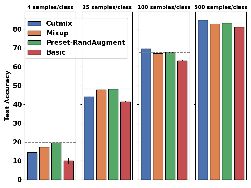
Figure 1: Performance of SotA augmentation methods on CIFAR 100 [26] trained with WideResnet-28-10 [46] for different number of training samples per class. Preset-RandAugment (green) performs better than MSDA (Cutmix[45] and Mixup[48]) with few training samples whereas the reverse is true with plentiful samples. As expected, the Basic augmentation that horizontally flips and crops the image has the lowest performance throughout.

We compare the performance of foundational augmentation techniques in Figure 1 and note that Preset-RandAugment has the best performance in low data regimes, with just 4-25 training samples per class. MSDA methods are not as effective with limited data as they are when data is abundant.

It is widely recognized that augmentations need to possess two crucial attributes: high diversity and realism [11], so that the augmented data represents a wide range of possible and plausible real-world scenarios.

Additionally, suitable inductive bias can yield faster model convergence and better generalization by restricting the model’s hypothesis space [17]. In limited data scenarios it is best to focus this bias on less class-specific patterns such as edges and textures, that is, to induce the model to learn stable low-level features in the early layers of a network. We formalize all the above properties below.

3.1 Definitions

Supervised training of a predictor $f\in F$ minimizes the risk (average loss) $R(f)=\mathbb{E}_{(\mathbf{x},\mathbf{y})\sim P}[l(f(\mathbf{x}),\mathbf{y})]$, over the data distribution $P(\mathbf{x},\mathbf{y})$ of the image and target class pairs. $P(\mathbf{x},\mathbf{y})$ is unknown, but a training dataset $\mathcal{D}_{e}=\{(\mathbf{x}_{i},\mathbf{y}_{i})\}_{i=1}^{m}$ that is randomly sampled from $P$ is available. $P(\mathbf{x},\mathbf{y})$ can thus be approximated by an empirical distribution $P_{e}(\mathbf{x},\mathbf{y})$ that places $m$ delta functions at $(\mathbf{x}_{i},\mathbf{y}_{i})$: $P_{e}(\mathbf{x},\mathbf{y})=\frac{1}{m}\sum_{i=1}^{m}\delta_{\mathbf{x}_{i}}(\mathbf{x})\delta_{\mathbf{y}_{i}}(\mathbf{y}).$

The quality of the approximation in $P_{e}$ is poor when $\mathcal{D}_{e}$ is either sparse or only covers a small part of the support of $P$. We can then estimate $P$ better using a vicinal distribution [4] $P_{a}(\tilde{\mathbf{x}},\tilde{\mathbf{y}}|\mathbf{x}_{i},\mathbf{y}_{i})$ that models the space of all augmented samples $(\tilde{\mathbf{x}},\tilde{\mathbf{y}})$ in the vicinity of $(\mathbf{x}_{i},\mathbf{y}_{i})$. A good augmentation generates $(\tilde{\mathbf{x}},\tilde{\mathbf{y}})$ that lie within the convex hull of the samples $({\mathbf{x}},{\mathbf{y}})\sim\mathcal{D}_{e}$. Thus, $P$ can be approximated better as: $P_{a}(\tilde{\mathbf{x}},\tilde{\mathbf{y}})=\sum_{i=1}^{m}P_{a}(\tilde{\mathbf{x}},\tilde{\mathbf{y}}|\mathbf{x}_{i},\mathbf{y}_{i})P(\mathbf{x}_{i},\mathbf{y}_{i})$ [4], and the augmented dataset $\mathcal{D}_{a}=\{(\tilde{\mathbf{x}}_{i},\tilde{\mathbf{y}}_{i})\}_{i=1}^{n}$ can be viewed as samples from $P_{a}$ [48]. Training then minimizes the vicinal risk $R_{v}(f)=\mathbb{E}_{(\tilde{\mathbf{x}},\tilde{\mathbf{y}})\sim P_{a}}[l(f(\tilde{\mathbf{x}}),\tilde{\mathbf{y}})]$.

The following properties of augmentation methods are valuable when $\mathcal{D}_{e}$ is very small:

1. High diversity is the average spread or variance of the vicinal distribution $P_{a}(\tilde{\mathbf{x}},\tilde{\mathbf{y}}|\mathbf{x}_{i},\mathbf{y}_{i})$ over all $(\mathbf{x}_{i},\mathbf{y}_{i})\in\mathcal{D}_{e}$. A wide spread ensures a denser coverage of $P$ around each original sample $({\mathbf{x}}_{i},{\mathbf{y}}_{i})$.

2. High similarity of $P_{a}$ to $P$: The augmented samples $(\tilde{\mathbf{x}},\tilde{\mathbf{y}})$ must be realistic and come from the true data distribution $P$. Since $P$ is unknown and approximated by $P_{e}$, we measure realism in $P_{a}$ by its similarity to $P_{e}$ as described in Section 3.3. Setting $P_{a}=P_{e}$ would achieve maximum realism in $P_{a}$ but at the expense of diversity (property 1), so we must strike a balance between these two properties.

3. Fast convergence through Low-level Feature Invariance: The neural function $f$ extracts low-level and high-level features from $\mathbf{x}$ in its early and later layers respectively: $f({\mathbf{x}})=(f^{l}({\mathbf{x}}),f^{h}({\mathbf{x}}))$. Augmented samples $(\tilde{\mathbf{x}},\tilde{\mathbf{y}})\sim P_{a}$ that are stable across similar ${\tilde{\mathbf{x}}}$ result in faster convergence to a better solution $f^{*}$. Stable $f^{l}({\tilde{\mathbf{x}}})$ are easier to achieve when training samples are sparse, since low-level feature information is class-agnostic and widely prevalent. It is harder to directly achieve stable $f^{h}({\tilde{\mathbf{x}}})$ with sparse samples.

In order to measure all the above properties, we sample $k$ times from $P_{a}(\tilde{\mathbf{x}},\tilde{\mathbf{y}}|\mathbf{x}_{i},\mathbf{y}_{i})$ around a data sample $(\mathbf{x}_{i},\mathbf{y}_{i})\in\mathcal{D}_{e}$ to produce an augmentation cloud $\prescript{k}{}{\mathcal{D}}_{a}^{i}$. In MSDA methods, $P_{a}(\tilde{\mathbf{x}},\tilde{\mathbf{y}}|\mathbf{x}_{i},\mathbf{y}_{i})$ depends on $(\mathbf{x}_{i},\mathbf{y}_{i})$ as well another sample $(\mathbf{x}_{j},\mathbf{y}_{j})$ drawn from $\mathcal{D}_{e}$. Further, $\mathcal{D}_{e}$ is split into training, validation and test datasets $\mathcal{T}_{e}$, $\mathcal{V}_{e}$ and $\mathcal{S}_{e}$. We analyze foundational augmentation methods in terms of these properties next and use $\mathcal{T}_{e}$, $\mathcal{V}_{e}$ from the CIFAR-100 dataset for this analysis. In all experiments, averages and errors are calculated across 3 distinctly seeded models.

3.2 Diversity

Method	Diversity
Preset-RandAugment	2516.78
Cutmix	1775.41
Mixup	1643.86
Basic	1141.87

Table 2: Diversity $\langle{\sigma_{a}^{2}}\rangle$ for different foundational augmentation methods on the CIFAR-100 dataset. Preset-RandAugment has the highest diversity.

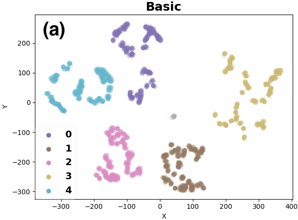
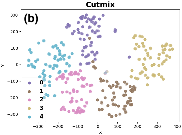
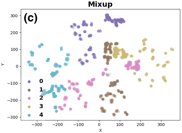
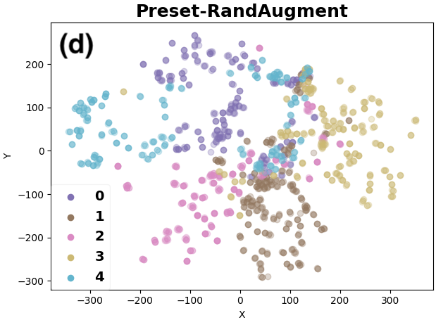
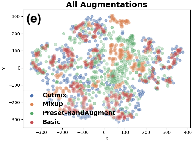
Figure 2: (a-d) Visualizing $\prescript{10,000}{}{\mathcal{D}}_{a}^{i}$ in 2D using t-SNE for 5 randomly drawn samples $x_{i}\in\mathcal{T}_{e}$ and for different augmentation methods. Plot (e) combines the clouds for all methods, with different colors for different methods. Preset-RandAugment’s (green) is the most dispersed in the embedding space.

All the foundational augmentation methods – Preset-RandAugment, Cutmix and Mixup – generate dynamic augmentations by generating augmentation parameters randomly in each training iteration. This stochasticity increases diversity and improves generalization over simple augmentations like flips and crops [9].

Cubuk et al. [11] measure the diversity of an augmentation method using the training risk (at convergence) of a model trained with it, based on the intuition that it is harder to overfit with more diverse data. However, the magnitude of the risk depends on other factors as well, such as the capacity of the model, size of the training set, optimization settings etc. Also, [31] found the claims made by [11] not to hold for more recent augmentation methods.

Instead, we measure diversity as the average variance of the vicinal distribution $P_{a}(\tilde{\mathbf{x}},\tilde{\mathbf{y}}|\mathbf{x}_{i},\mathbf{y}_{i})$ around a data sample $(\mathbf{x}_{i},\mathbf{y}_{i})\in\mathcal{T}_{e}$. We compute the augmentation cloud $\prescript{k}{}{\mathcal{D}}_{a}^{i}$ with $k=10,000$, reduce it to 100 dimensions with PCA [43], and compute the variance $(\sigma_{a}^{2})^{i}$ of the reduced point cloud. Diversity, denoted by $\langle{\sigma_{a}^{2}}\rangle$, is the average $(\sigma_{a}^{2})^{i}$ over all $(\mathbf{x}_{i},\mathbf{y}_{i})\in\mathcal{T}_{e}$, shown for different methods in Table 2. We measure diversity around a single image sample for Preset-RandAugment, and a pair of images for MSDA. Figure 2 (a-e) visualizes the point clouds for some random samples from $\mathcal{T}_{e}$ in 2D using t-SNE embeddings [41].

Preset-RandAugment’s augmentations has higher diversity (Table 2) compared to MSDA. It uses photometric operations like equalize, contrast, color and brightness adjustments that redistribute and shift pixel intensities (Figure 2(d-e)) and increase model invariance to real-world lighting variations. The next section shows that despite this higher diversity, Preset-RandAugment’s outputs are realistic and close to the true distribution $P$.

3.3 Similarity to True Distribution

An augmentation method must strike a balance between producing diverse samples and ensuring that those samples are still realistic and relevant. A sample in $P_{a}$ is realistic when it comes from the true distribution $P$, which $P_{e}$ approximates. So we measure the similarity of $P_{a}$ to $P_{e}$.

Several strategies are used in literature to measure distributional similarity [29, 11, 15]. Facciolo et al. [15] train unsupervised variational auto-encoders (VAEs) on the real and the augmented data and measure the similarity between the learned representations by mutual information. Training a VAE is cumbersome and the resulting measure relies heavily on the VAE generating good quality samples.

Other methods [29, 11] train a model on the clean training data $\mathcal{T}_{e}$, and measure its accuracy on an augmented validation set $\prescript{1}{}{\mathcal{D}}_{a}^{\mathcal{V}}=\bigcup_{i}\{\prescript{1}{}{\mathcal{D}}_{a}^{i}:(\mathbf{x}_{i},\mathbf{y}_{i})\in\mathcal{V}_{e}\}$, the aggregate of all the individual augmentation clouds for each point in $\mathcal{V}_{e}$. The hypothesis is that if the pattern of the data $\prescript{1}{}{\mathcal{D}}_{a}^{\mathcal{V}}$ generated by a given method follows that of $\mathcal{V}_{e}$, then their validation accuracies will be close.

In contrast, we use the cross entropy score instead of accuracy. Accuracy computation requires a single predicted label for an input. However, MSDA makes soft labels for pairs of mixed images. Computing accuracy requires thresholding these soft labels and can produce incorrect results, making cross entropy more appropriate in this case.

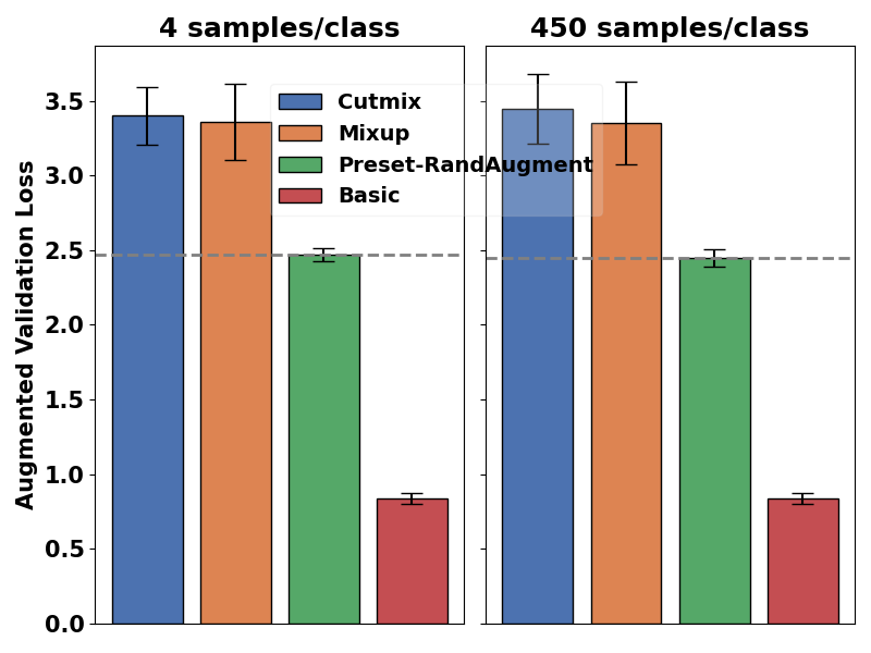
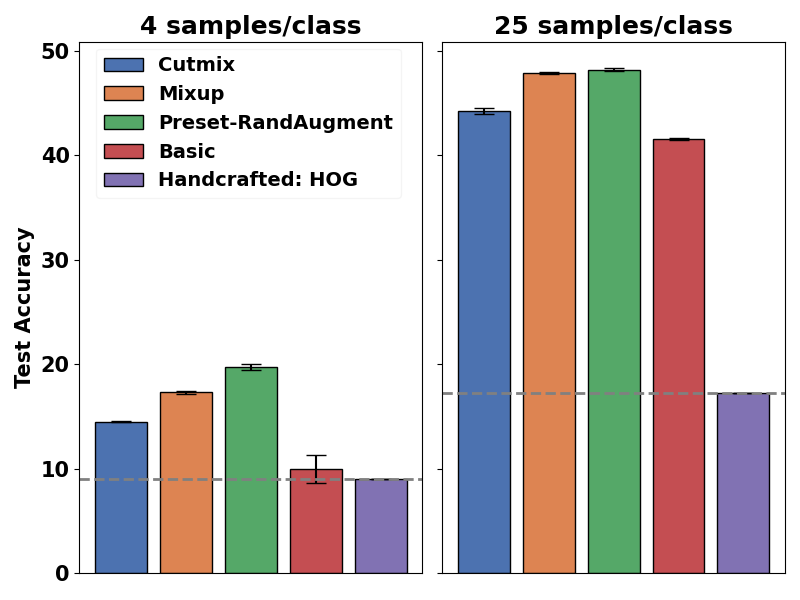
(a)	(b)

Figure 3: (a) Distributional similarity of samples from different augmentation methods to $P_{e}$, measured by the cross entropy risk ($\downarrow$) on an augmented validation set $\prescript{1}{}{\mathcal{D}}_{a}^{\mathcal{V}}$. (b) Comparing a simple classifier learned with handcrafted features with foundational augmentation methods trained with CNNs.

We measure distributional similarity of an augmentation distribution $P_{a}$ to the empirical distribution $P_{e}$ by the cross entropy risk $R(f^{*})=\mathbb{E}_{(\tilde{\mathbf{x}},\tilde{\mathbf{y}})\sim\prescript{1}{}{\mathcal{D}}_{a}^{\mathcal{V}}}[l(f^{*}(\tilde{\mathbf{x}}),\tilde{\mathbf{y}})]$ of a model $f^{*}$ trained on the clean $\mathcal{T}_{e}$, when it has sparse and abundant data. Figure 3(a) shows that Basic Augmentation (flips and crops) samples have the lowest risk, and are closest to $P_{e}$, followed by Preset-RandAugment. On the other hand, Cutmix and Mixup samples are the farthest from $P_{e}$.

In contrast to MSDA samples, Preset-RandAugment samples preserve the high-level semantics of the object, causing the model to perceive them to be more realistic. Further, Preset-RandAugment generates augmentations insensitive to changes in lighting and viewpoint. Figure 4 shows examples from both types of methods.

(a) Input	(b) Preset-RandAugment		(c) Mixup	(d) Cutmix

Figure 4: For an example from the poodle and van classes, Preset-RandAugment samples model real-world changes like rotations and lighting variations, and preserve high-level object information. On the other hand, MSDA samples dilute semantic information and appear unrealistic.

3.4 Low-Level Feature Invariance

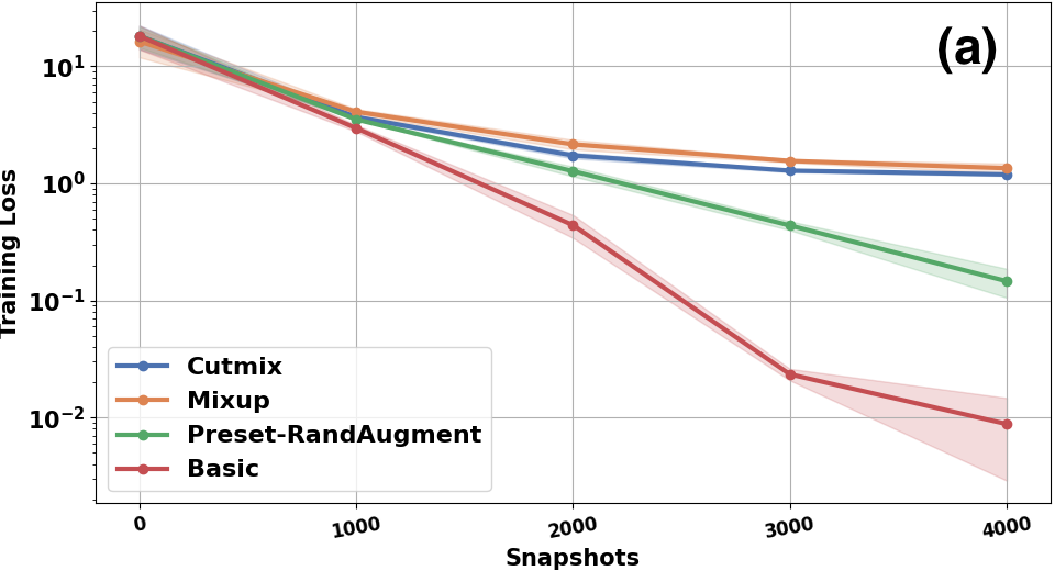
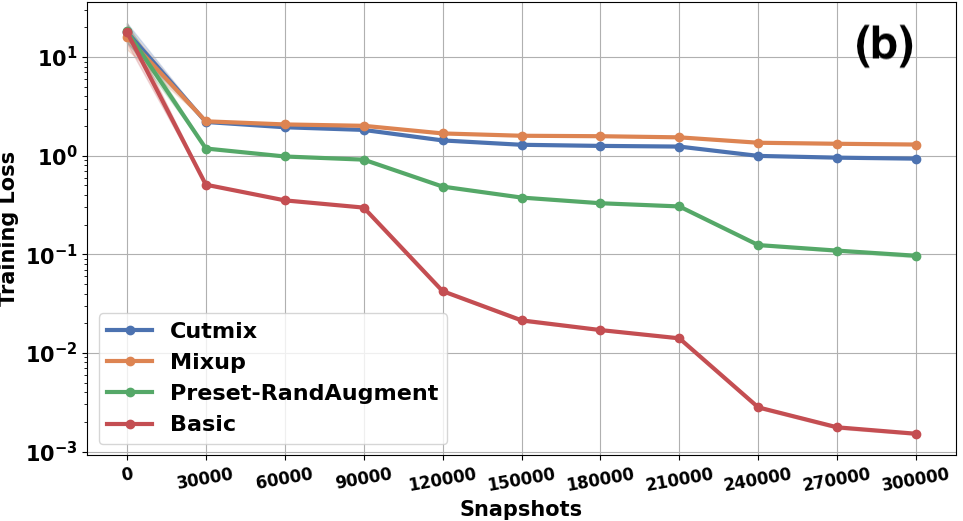
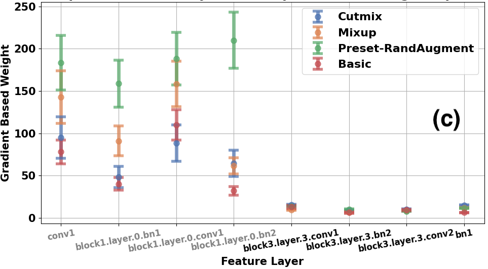
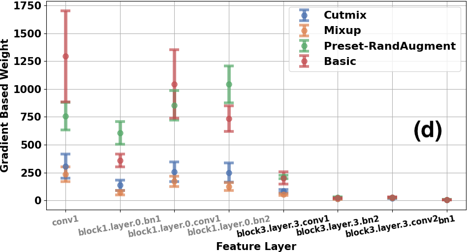
Figure 5: (a-b) Learning curve for different augmentation methods, and for (a) sparse (4 per class) and (b) abundant (450 per class) training samples. (c-d) Gradient based weights $w_{r}^{c}$ averaged over all samples $(\mathbf{x},\mathbf{y})\in\mathcal{V}_{e}$, and over 3 differently seeded models is shown for 4 lowest (gray) and highest (black) feature maps in the model. The model in (c) is trained with sparse (4 per class) samples and in (d) it is trained with abundant (450 per class) samples.

Augmentation samples ${\tilde{\mathbf{x}}}$ that encourage the model to learn invariant features $f({\tilde{\mathbf{x}}})$ lead to faster convergence and better generalization [17]. It is easier to achieve low-level feature $f^{l}({\tilde{\mathbf{x}}})$ stability due to the ubiquity of low-level information in sparse data settings, as detailed in Section 3.1.

The convergence rate is measured from the plots of risk $R(f)$ versus training iteration, shown in Figure 5(a-b). The model $f$ is trained on $\prescript{k}{}{\mathcal{D}}_{a}^{\mathcal{T}}=\bigcup_{i}\{\prescript{k}{}{\mathcal{D}}_{a}^{i}:(\mathbf{x}_{i},\mathbf{y}_{i})\in\mathcal{T}_{e}\}$. Preset-RandAugment models converge consistently faster than MSDAs with both limited (4 per class) and plentiful (450 per class) training data. Preset-RandAugment is based on low-level feature manipulations that lead to model invariance to such changes. In contrast, the blending operations and sharp discontinuities in MSDA methods dilute low-level and high-level semantic information (Figure 4). This makes it harder for the network to learn stable features.

Promoting Convergence Improves Generalization

We show that improving the training speed of the MSDA method, Cutmix, results in better generalization. The Basic augmentations enable fast model convergence (Figure 5(a-b)). We inject these augmentations during the first 10,000 iterations of training and then present Cutmix samples for the remainder. This process is motivated by curriculum learning [2], and shows that promoting convergence even during just the early part of training can improve the generalization of Cutmix. See Table 3.

Aug	Accuracy (%, $\uparrow$)	Risk at 50K iterations ($\downarrow$)
Cutmix	14.50$\pm$0.04	0.67 $\pm$0.21
Cutmix-Faster	15.32$\pm$0.39	0.54 $\pm$0.13

Table 3: For 4 samples/class, introducing Basic augmentations in Cutmix-Faster enables faster convergence (lower risk at 50K iterations) and better accuracy than Cutmix.

Impact of Learned Low-level Features on Output Prediction

We use Gradient-weighted Class Activation Mapping (Grad-CAM) [37] to show that models that converge faster also learn more impactful low-level features. Grad-CAM is a model interpretability tool that reveals the feature maps in the model that most influence the model’s prediction. It computes the gradient of the model’s score for a target class $c$ with respect to the feature map and global-average-pools it to obtain a single weight $w_{r}^{c}$ per feature map $f^{r}$. This weight measures the sensitivity of the score for class $c$ to changes in the feature map $f^{r}$. We compute $w^{c}$ using the ground-truth class $\mathbf{y}^{c}=1$, when the model’s maximum prediction aligns with the true class, i.e. $\hat{\mathbf{y}}^{c}=\mathbf{y}^{c}$. Figure 5(c-d) shows $w_{r}^{c}$ for $r=l$ low-level and $r=h$ high-level feature maps in various scenarios.

For models trained with Preset-RandAugment on both sparse and plentiful data, low-level features $f^{r=l}$ have a significant influence on the model’s correct predictions. With them, Preset-RandAugment model achieves fast convergence (Figure 5(a-b)) and generalizes better (Figure 1).

The Basic augmentation model, which also converges fast, learns good $f^{l}$ when the data is plentiful. However for sparse data, these augmentations have very low diversity (Table 2) and end up overfitting.

Mixup models learn more impactful $f^{l}$ compared to Cutmix and also generalize better than it. It seems that the blended images in Mixup dilute $f^{h}$, preventing the network from relying on them. However, edges and gradients are still present, forcing the network to rely more on $f^{l}$.

Invariant Low-Level Features Aid Generalization

Low-level features providing photometric and geometric invariance, such as Scale Invariant Feature Transform (SIFT) [30], Histogram of Oriented Gradients (HOG) [13] etc., were key in the pre-deep learning era for generalization with scarce data. In Figure 3(b), we compare the foundational augmentations trained on deep CNNs against the HOG + SVM (Support Vector Machines) approach. The manually designed features are almost on par with deep features trained using Basic augmentation when data is very scarce (only 4 per class). This highlights the generalization power of low-level feature invariance when working with limited data. We note that with more data (25 per class) deep features easily overpower handcrafted features. Preset-RandAugment uses low-level transforms and deep features, and excels in the sparse data regime.

3.5 Preset-RandAugment Effectiveness

Thus, the performance of an augmentation method depends on a tradeoff between (1) diversity, (2) realism, (3) invariant low-level feature learning. Preset-RandAugment is the most diverse among foundational methods and ranks second in both distributional similarity and convergence rate. Its good balance among all 3 properties makes it particularly effective when training data is limited.

The key contributor to Preset-RandAugment’s performance is its use of photometric and geometric transforms. These low-level feature transforms produce augmentations that are diverse, realistic, and promote low-level feature invariance, which speeds up model convergence.

On the other hand, MSDA samples provide regularization, reduce overfitting, [49, 35, 34] and enable better generalization by learning smoother decision boundaries [32, 6]. These properties are complementary to that of Preset-RandAugment and can be combined to produce better generalization, as we discuss next.

4 RandMSAugment

RandMSAugment is a novel augmentation that integrates the complementary, key operations of foundational methods to produce better generalization. We showed earlier the critical role of low-level feature transforms in Preset-RandAugment. We combine this with two key operations used to mix samples in MSDA methods: linear interpolation, (Mixup, Manifold Mixup, HMix, GMix etc.) and cut-and-paste (Cutmix, ResizeMix etc.). To preserve salient object information in the mixed sample, we choose the efficient and parameter-tuning-free idea of resize-and-paste proposed in ResizeMix [36], which cuts, resizes, and pastes the entire first image in a random location in the second.

1

Data: $\mathbf{x}_{1},\mathbf{x}_{2}\leftarrow\text{images}$, $\mathbf{y}_{1},\mathbf{y}_{2}\leftarrow\text{labels}$

Result: $\mathbf{x}^{M}_{1,2},\mathbf{y}^{M}_{1,2}$

2

3

4 Function Choice($S$, $n$[1]):

5       $s\leftarrow$ select $n$ elements from $S$ with uniform probability

6       return $s$

7      

8Function FeatXform($\mathbf{x},\mathbf{y},\boldsymbol{\ell}[\text{None}],\boldsymbol{\theta}[\text{None}]$):

9       $\mathcal{L}\leftarrow\text{Set of 14 low-level transforms from }$ [10]

10       $\Theta\leftarrow\text{Magnitude Range for each }\mathcal{L}$ from [10]

11       if $\mathbf{l,\theta}$ is not None then

12             $\boldsymbol{\ell},\boldsymbol{\theta}\leftarrow$ Choice($L$, 2), Choice($\Theta$, 2)

13            

14      $\mathbf{x}^{ft}\leftarrow$ SequentialApply($\mathbf{x},\boldsymbol{\ell},\boldsymbol{\theta}$)

15       return $\mathbf{x}^{ft},\mathbf{y},\boldsymbol{\ell},\boldsymbol{\theta}$

16      

17Function Interp($\mathbf{x}_{1},\mathbf{x}_{2},\mathbf{y}_{1},\mathbf{y}_{2}$):

18       $\lambda\leftarrow$ Choice([0:1])

19       $\mathbf{x}^{ip}_{1,2},\mathbf{y}^{ip}_{1,2}=\lambda(\mathbf{x}_{1},\mathbf{y}_{1})+(1-\lambda)(\mathbf{x}_{2},\mathbf{y}_{2})$

20       return $\mathbf{x}^{ip}_{1,2},\mathbf{y}^{ip}_{1,2}$

21      

22Function ReszPst($\mathbf{x}_{1},\mathbf{x}_{2},\mathbf{y}_{1},\mathbf{y}_{2},\lambda_{s}[\text{None}]$):

23       if $\lambda_{s}$ is not None then

24             ${\lambda_{s}}\leftarrow$ Choice([0:1])

25      $p,q\leftarrow$ Choice([0: $x_{w}$]), Choice([0:$x_{h}$])

26      

27      $\mathcal{M}\leftarrow$ MixingMask($(p,q),(x_{w},x_{h}),\lambda_{s}$)

28       $\mathbf{x}^{rp}_{1,2}=\mathcal{M}\odot$ Resize($\mathbf{x}_{1},\lambda_{s}$) + $(1-\mathcal{M})\odot\mathbf{x}_{2}$

29       $\mathbf{y}^{rp}_{1,2}=\lambda_{s}\mathbf{y}_{1}+(1-\lambda_{s})\mathbf{y}_{2}$

30       return $\mathbf{x}^{rp}_{1,2},\mathbf{y}^{rp}_{1,2}$

31      

Algorithm 1 Components of RandMSAugment

We combine the set of operations, [FeatXform, Interp, ReszPst] in a way that is inspired by Preset-RandAugment. We choose two operations from the set uniformly at random in every training iteration, and apply them sequentially to the image. The operation parameters are also chosen uniformly at random from a predefined range or using hyperparameters recommended by each method’s first paper. These additional layers of stochasticity in the combination process improve the diversity of the mixed samples. Our method has no new hyperparameters, requires no validation data, and involves no cumbersome optimizations.

4.1 Component Functions

Let $\mathbf{x}_{1},\mathbf{x}_{2}\in\mathbb{R}^{m}$ be two images with one-hot vector class label $\mathbf{y}_{1},\mathbf{y}_{2}\in\mathbb{R}^{C}$, where $C$ is the number of classes. In FeatXform, two operations $\boldsymbol{\ell}$ are chosen from a set of low level operations $\mathcal{L}$ (rotation, equalizing etc.). Their magnitudes $\boldsymbol{\theta}$ are also randomly chosen from a range of values $\Theta$, where $\mathcal{L}$ and $\Theta$ are defined by [10]. The operations $\boldsymbol{\ell}$ are applied sequentially to $\mathbf{x}$. These low level transforms do not affect the label $\mathbf{y}$. In Interp, mixed samples are generated as the convex combination of two images (and their labels), $\mathbf{x}_{1}$ ($\mathbf{y}_{1}$) and $\mathbf{x}_{2}$ ($\mathbf{y}_{2}$) in $\mathbb{R}^{m}$ (and $\mathbb{R}^{C}$). The mixing coefficient $0\leq\lambda\leq 1$ is randomly sampled from $\text{Beta}(\alpha,\alpha)$, with parameter $\alpha$ specified in [48]. The ReszPst method first computes a binary mask $\mathcal{M}$ at a randomly chosen paste box location $(p,q)$ within the image $\mathbf{x}$ with a relative area $\lambda_{s}$. The scale factor $0\leq\lambda_{s}\leq 1$ is chosen randomly from a range specified in [36]. ReszPst resizes $\mathbf{x}_{1}$ by a factor of $\lambda_{s}$ and then combines it with $\mathbf{x}_{2}$ using mask $\mathcal{M}$. The mixed label is obtained as the weighted vector sum of the original labels, with the weights determined by the proportions of the merged areas. All these component functions are defined in Algorithm 1.

4.2 Combination

At every training iteration, RandMSAugment draws two operations randomly from [FeatXform, Interp, ReszPst] .

If the chosen operations are [FeatXform, Interp], we apply FeatXform with the same randomly chosen parameters $\boldsymbol{\ell,\theta}$ to both images $\mathbf{x}_{1}$ and $\mathbf{x}_{2}$ and then Interp them. This is because interpolating images from different feature spaces can degrade objectness information, resulting in unrealistic images that are hard for the network to learn from.

For [FeatXform, ReszPst] we apply FeatXform to $\mathbf{x}_{1}$ and $\mathbf{x}_{2}$ with independent randomly chosen parameters. Since patches from $\mathbf{x}_{1}$ and $\mathbf{x}_{2}$ are juxtaposed (and not interpolated), the information in them is preserved even when they come from different feature spaces. We add another layer of randomness by randomly choosing between the transformed image $\mathbf{x}^{ft}_{t}$ and the original image $\mathbf{x}_{t}$. Images thus selected are combined with ReszPst with random $\lambda_{s}$.

For [Interp, ReszPst], we first use Interp to make the interpolated image $\mathbf{x}^{ip}_{1,2}$. We then mix $\mathbf{x}^{ip}_{1,2}$ with one of $\mathbf{x}_{1}$ or $\mathbf{x}_{2}$ using ReszPst. We would like $\mathbf{x}^{ip}_{1,2}$ to occupy a significant portion of the mixed sample. So, based on the value of the random scale factor $\lambda_{s}$, we make $\mathbf{x}^{ip}_{1,2}$ the first or second of the samples to be mixed by ReszPst. Algorithm 2 outlines these methods, with a visual description in Section 7.1. Figure 6 shows examples augmentations.

The two crucial aspects in RandMSAugment are the use of effective, complementary, yet simple component functions, and the extensive use of randomness in mixing. The precise details in combining the component functions are less important. We show in Section 7.2 that an alternate way to combine [Interp, ReszPst] has similar performance.

Data: $\mathbf{x}_{1},\mathbf{x}_{2}\leftarrow\text{images}$, $\mathbf{y}_{1},\mathbf{y}_{2}\leftarrow\text{labels}$

Result: $\mathbf{x}^{M}_{1,2},\mathbf{y}^{M}_{1,2}$

1

2

3

4Function RandMixAugment($\mathbf{x}_{1},\mathbf{x}_{2},\mathbf{y}_{1},\mathbf{y}_{2}$):

5      

6      $\mathcal{O}\leftarrow$ [FeatXform, Interp, ReszPst ]

7       $\mathbf{o}\leftarrow$ Choice($\mathcal{O},2$)

8       if $\mathbf{o}$ in [FeatXform, Interp ]  then

9             $\mathbf{x}^{ft}_{1},\mathbf{y}^{ft}_{1},\boldsymbol{\ell},\boldsymbol{\theta}\leftarrow$ FeatXform($\mathbf{x}_{1},\mathbf{y}_{1}$)

10             $\mathbf{x}^{ft}_{2},\mathbf{y}^{ft}_{2}\leftarrow$ FeatXform($\mathbf{x}_{2},\mathbf{y}_{2},\boldsymbol{\ell},\boldsymbol{\theta}$)

11             $\mathbf{x}^{M}_{1,2},\mathbf{y}^{M}_{1,2}\leftarrow$ Interp($\mathbf{x}^{ft}_{1},\mathbf{x}^{ft}_{2},\mathbf{y}^{ft}_{1},\mathbf{y}^{ft}_{2}$)

12      if $\mathbf{o}$ in [FeatXform, ReszPst ]  then

13            

14            for $t=1$ to $2$ do

15                   $\mathbf{x}^{ft}_{t},\mathbf{y}^{ft}_{t}\leftarrow$ FeatXform($\mathbf{x}_{t},\mathbf{y}_{t}$)

16                   $\mathbf{x}^{r}_{t}\leftarrow$ Choice($[\mathbf{x}^{ft}_{t},\mathbf{x}_{t}]$)

17                  

18            $\mathbf{x}^{M}_{1,2},\mathbf{y}^{M}_{1,2}\leftarrow$ ReszPst($\mathbf{x}^{r}_{1},\mathbf{x}^{r}_{2},\mathbf{y}^{ft}_{1},\mathbf{y}^{ft}_{2}$)

19      if $\mathbf{o}$ in [Interp, ReszPst ]  then

20             $\mathbf{x}^{ip}_{1,2},\mathbf{y}^{ip}_{1,2}\leftarrow$ Interp($\mathbf{x}_{1},\mathbf{x}_{2},\mathbf{y}_{1},\mathbf{y}_{2}$)

21             ${\lambda_{s}}\leftarrow$ Choice([0:1])

22             if ${\lambda_{s}}>0.5$  then

23                   $\mathbf{x}^{M}_{1,2},\mathbf{y}^{M}_{1,2}\leftarrow$ ReszPst($\mathbf{x}^{ip}_{1,2},\mathbf{x}_{2},\mathbf{y}^{ip}_{1,2},\mathbf{y}_{2},{\lambda_{s}}$)

24            else

25                  $\mathbf{x}^{M}_{1,2},\mathbf{y}^{M}_{1,2}\leftarrow$ ReszPst($\mathbf{x}_{1},\mathbf{x}^{ip}_{1,2},\mathbf{y}_{1},\mathbf{y}^{ip}_{1,2},{\lambda_{s}}$)

26            return $\mathbf{x}^{M}_{1,2},\mathbf{y}^{M}_{1,2}$

27            

Algorithm 2 RandMSAugment

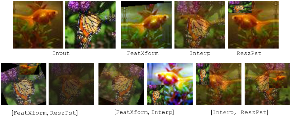
Figure 6: The first row shows example input images and augmented samples from the component functions used in our method. The second row shows example augmentations for every pair of component operations, which are all samples from RandMSAugment. Our samples are diverse and exhibit real-world lighting and geometric changes.

5 Experiments

We evaluate RandMSAugment for image classification on STL-10 [8], CIFAR-100 [26], and Tiny-Imagenet datasets [7], with 5,000, 50,000, and 100,000 training samples respectively. We run experiments on the full and limited data settings. For limited data, we randomly sample various amounts from the full dataset in a class-balanced manner, similar to SSL methods[39, 47]. However, unlike SSL methods, we do not use unlabelled data, as our goal is to understand and leverage the potential of fully supervised methods for sparse data problems. Using unlabelled data is complementary to our approach.

Methods

We compare RandMSAugment to recent SotA techniques that use no additional data for augmentation: Basic (flips and crops), Mixup [48], Cutmix [45], Preset-RandAugment (Section 1), ResizeMix [36], Augmix [20], AutoMix [52], HMix and GMix [34]. The neural module in Automix requires several thousands more parameters than the baseline architecture used in other methods (Table 7.3), as indicated with ^∗ in the comparison tables.

Settings

For a fair comparison, we ran experiments for all methods with the same training settings [33] in TorchSSL [47]. Following standard practice [10], we use a WRN 28-10 [46] for CIFAR-100, WRN 28-2 variant [51] for STL-10 and PreAct-ResNet18 [19] for Tiny-Imagenet. We train models for $2^{20}$ iterations when using all the data. With sparse data, we train for 500K iterations, to be fair to methods with different convergence speeds. For each method we report the best accuracy from the last 20 snapshots [47]. We use SGD with momentum 0.9, weight decay 0.0005, and batch size 64. We use the MultistepLR schedule with an initial learning rate 0.03, gamma 0.3 and step ratio 0.1. We perform an exponential moving average with decay factor 0.999.

For the component augmentations used in our method, we use default parameters specified by the methods that proposed them. We use the same set of low-level transforms specified in Preset-RandAugment, with N=2 and randomly sample M from the full range of magnitudes. For Mixup, we draw $\lambda$ from a Beta distribution with $\alpha=1.0$ for CIFAR-100 and STL-10, and $\alpha=0.2$ for Tiny-Imagenet, as in [48]. The ResizeMix resize-factor is random in (0.2,0.8).

5.1 Performance

We compare the methods in terms of the Top-1 accuracy rate, and report the mean and standard deviation over 3 independent networks trained with different random seeds in Tables 4-6. The best method is shown in bold and the second best is underlined. We also show results of models trained with our intermediate combinations: [FeatXform, ReszPst] abbreviated as [FT, RP ], [FeatXform, Interp] abbreviated as [FT, IP ], and RandMSAugment^-, which randomly chooses between [FT, RP ] and [FT, IP ]. This combination emphasizes FeatXform, which we showed in Section 3 to be effective on sparse training data.

Our RandMSAugment performs the best on all 3 datasets. We also show the gain in performance in terms of percentage points over the second best method (underlined). The gains are most dramatic for sparse samples (4, 25, 100 samples / class), ranging from 4.1% (Tiny-Imagenet) to 6.75% (STL-10). We also improve performance when the samples are abundant (500 samples / class), with gains ranging from 1.03 % (CIFAR-100) to 2.47 % (STL-10).

STL-10 has only 10 classes, so there are only 40 samples in total for the sparsest case (versus 400 in CIFAR-100 and 800 in Tiny-Imagenet). Here, the FeatXform based method, Preset-RandAugment performs especially well, and so emphasizing FeatXform in RandMSAugment^- is more beneficial than RandMSAugment.

Table 4: Top-1 accuracy (%, $\uparrow$) on CIFAR-100 (100 classes). [FT, RP ] and [FT, IP ] are our intermediate outputs.

Augmentation	Samples / Class
	4	25	100	500
Basic	9.93$\pm$1.36	41.57$\pm$0.08	63.30$\pm$0.10	81.16$\pm$0.03
Cutmix	14.50$\pm$0.04	44.27$\pm$0.28	69.80$\pm$0.06	84.95$\pm$0.15
ResizeMix	13.84$\pm$0.18	45.74$\pm$0.47	70.09$\pm$0.23	85.25$\pm$0.19
Mixup	17.31$\pm$0.17	47.87$\pm$0.10	67.21$\pm$0.04	82.93$\pm$0.20
Preset-RandAugment	19.74$\pm$0.25	48.21$\pm$0.18	67.69$\pm$0.04	83.43$\pm$0.10
Augmix	14.58$\pm$0.44	40.53$\pm$0.55	64.02$\pm$0.16	81.29$\pm$0.06
HMix	18.57$\pm$0.13	50.06$\pm$0.05	69.20$\pm$0.09	84.31$\pm$0.10
GMix	20.02$\pm$0.11	48.34$\pm$0.04	68.89$\pm$0.24	84.24$\pm$0.12
AutoMix∗	16.16$\pm$0.01	48.02$\pm$1.29	69.03$\pm$0.02	85.03$\pm$0.24
[FT, RP ]	22.21$\pm$0.05	53.29$\pm$0.17	72.19$\pm$0.08	86.13$\pm$0.13
[FT, IP ]	21.58$\pm$0.19	51.45$\pm$0.07	69.64$\pm$0.15	84.14$\pm$0.29
RandMSAugment-	25.07$\pm$0.10	53.87$\pm$0.02	72.04$\pm$0.07	85.87$\pm$0.03
RandMSAugment	24.27$\pm$0.26	54.44$\pm$0.06	72.67$\pm$0.03	86.28$\pm$0.24
Gains	+ 5.06$\pm$0.21	+ 4.37$\pm$0.02	+ 2.58$\pm$0.25	+ 1.03$\pm$0.29

Table 5: Top-1 accuracy (%, $\uparrow$) on STL-10 (10 classes).

Augmentation	Samples / Class
	4	25	100	500
Basic	22.28$\pm$0.70	37.03$\pm$0.56	66.37$\pm$0.26	85.77$\pm$0.20
Cutmix	24.17$\pm$0.52	47.88$\pm$0.34	68.01$\pm$0.54	90.62$\pm$0.12
ResizeMix	23.59$\pm$0.49	47.78$\pm$0.35	70.23$\pm$0.26	91.25$\pm$0.07
Mixup	29.40$\pm$0.16	55.35$\pm$0.35	73.06$\pm$0.15	89.88$\pm$0.07
Preset-RandAugment	39.77$\pm$0.17	63.40$\pm$0.43	77.88$\pm$0.14	91.21$\pm$0.13
Augmix	29.35$\pm$0.43	50.10$\pm$0.37	66.50$\pm$0.09	87.05$\pm$0.10
HMix	30.43$\pm$0.39	57.26$\pm$0.06	75.99$\pm$0.19	91.58$\pm$0.09
GMix	31.66$\pm$0.19	57.39$\pm$0.23	74.04$\pm$0.46	90.82$\pm$0.03
AutoMix∗	33.39$\pm$0.19	56.05$\pm$0.26	74.21$\pm$0.14	90.74$\pm$0.05
[FT, RP ]	42.56$\pm$0.70	67.97$\pm$0.42	82.70$\pm$0.15	93.24$\pm$0.16
[FT, IP ]	43.70$\pm$0.37	64.32$\pm$0.24	80.47$\pm$0.21	92.55$\pm$0.17
RandMSAugment-	45.01$\pm$0.28	70.14$\pm$0.51	83.81$\pm$0.12	94.02$\pm$0.06
RandMSAugment	43.50$\pm$0.35	68.83$\pm$0.07	83.67$\pm$0.17	94.05$\pm$0.05
Gains	+ 5.24$\pm$0.14	+ 6.75$\pm$0.84	+ 5.94$\pm$0.26	+ 2.47$\pm$0.06

Table 6: Top-1 accuracy (%, $\uparrow$) on Tiny-Imagenet (200 classes).

Augmentation	Samples / Class
	4	25	100	500
Basic	6.08$\pm$0.23	25.79$\pm$0.14	45.03$\pm$0.13	64.40$\pm$0.17
Cutmix	8.13$\pm$0.08	25.85$\pm$0.05	45.20$\pm$0.83	67.52$\pm$0.04
ResizeMix	7.80$\pm$0.10	25.69$\pm$0.13	46.06$\pm$0.57	67.77$\pm$0.22
Mixup	7.92$\pm$0.16	27.30$\pm$0.46	47.91$\pm$0.24	66.02$\pm$0.25
Preset-RandAugment	10.54$\pm$0.13	29.43$\pm$0.10	49.00$\pm$0.15	67.47$\pm$0.10
Augmix	9.51$\pm$0.10	26.51$\pm$0.26	45.29$\pm$0.47	64.57$\pm$0.28
HMix	7.96$\pm$0.31	26.80$\pm$0.89	46.11$\pm$0.34	67.71$\pm$0.42
GMix	10.05$\pm$0.17	26.21$\pm$0.20	46.49$\pm$0.40	67.61$\pm$0.34
Automix∗	8.14$\pm$0.36	23.30$\pm$0.29	45.75$\pm$0.50	66.81$\pm$0.20
[FT, RP ]	11.62$\pm$0.15	31.94$\pm$0.15	49.70$\pm$0.25	69.36$\pm$0.33
[FT, IP ]	11.53$\pm$0.10	32.03$\pm$0.41	50.82$\pm$0.10	67.81$\pm$0.29
RandMSAugment-	14.63$\pm$0.31	33.88$\pm$0.13	52.11$\pm$0.50	69.70$\pm$0.05
RandMSAugment	14.48$\pm$0.27	34.61$\pm$0.22	52.37$\pm$0.09	69.96$\pm$0.27
Gains	+ 4.10$\pm$0.39	+ 5.18$\pm$0.30	+ 3.37$\pm$0.23	+ 2.19$\pm$0.13

5.2 Ablation study

We compare the relative importance of the different components of our method via Top-1 accuracy in Table 7. The top part of the table shows that that FeatXform is the most effective individual component. Among pairwise combinations (middle part), [FeatXform, ReszPst] works best. The bottom part shows that balancing the 3 components yields the best results versus emphasizing any one of them.

We illustrate the augmentation properties (Section 3) of RandMSAugment, and show additional experiments with different parameters and training settings in Sections 7.4, 7.5 and 7.6 respectively. Code is also attached with the Supplementary material.

Table 7: Top-1 accuracy (%, $\uparrow$) on CIFAR-100 for 25 samples / class. Orange ticks flag emphasized components in the mix.

FeatXform	ReszPst	Interp	Top-1 Accuracy
✓			48.32$\pm$0.36
	✓		46.62$\pm$0.30
		✓	47.85$\pm$0.19
✓	✓		53.29$\pm$0.17
✓		✓	51.45$\pm$0.07
✓	✓		50.23$\pm$0.09
✓	✓	✓	53.83$\pm$0.03
✓	✓	✓	54.39$\pm$0.08
✓	✓	✓	53.30 $\pm$0.11
✓	✓	✓	54.46$\pm$0.05

6 Conclusion

We evaluated foundational augmentation methods for data-scarce scenarios based on 3 important properties: diversity, realism, and the one we introduced: fast convergence via feature invariance. We showed that Preset-RandAugment strikes an optimal balance among them, using low-level feature transforms as its key component. We proposed a novel technique, RandMSAugment, which combines these low-level transforms with the complementary strengths of MSDA methods. We showed through extensive comparisons over 3 datasets and ablation studies that our efficient method produces dramatic gains over the competition for sparse samples and more moderate gains for abundant data. Our method operates in the fully-supervised scenario. We plan to explore RandMSAugment for SSL in future work.

Supplementary Material

7 Additional Experiments

7.1 Visual Description of Algorithm

Figure 7 is a visual demonstration of Algorithm 2.

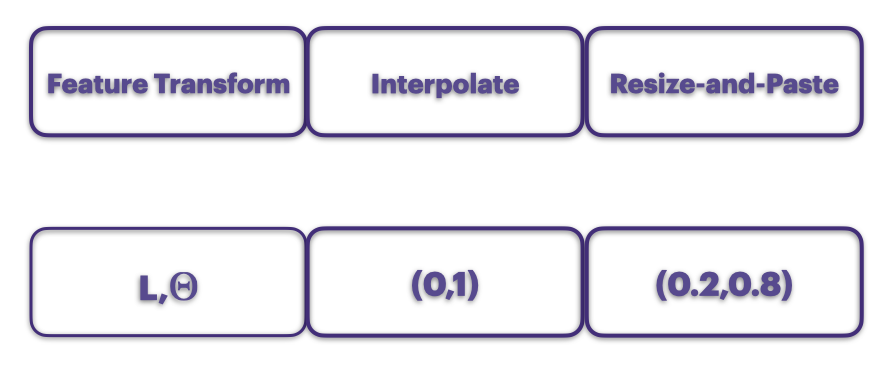
(a)

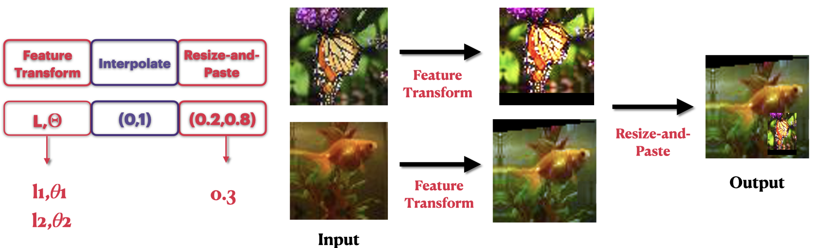
(b)

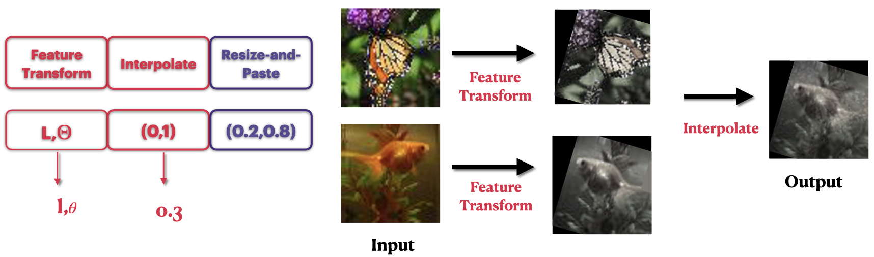
(c)

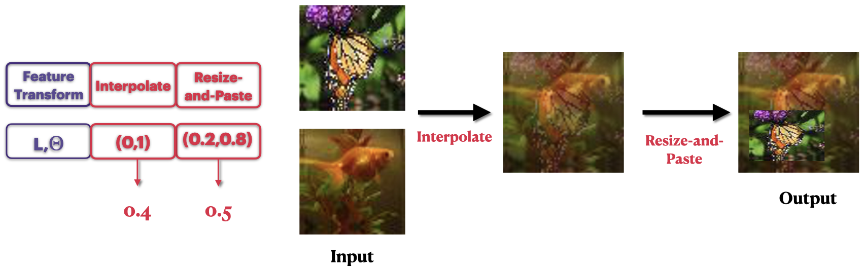
(d)

Figure 7: (a) The different component operations in RandMSAugment. In each training iteration, we randomly choose two operations out of them. Their associated parameters are also chosen from pre-defined ranges, uniformly at random. We show an example for [FeatXform, ReszPst ] in (b), [FeatXform, Interp ] in (c), and [Interp, ReszPst ] in (d).

7.2 Alternate Way to Combine [Interp, ReszPst]

The two crucial aspects in RandMSAugment are the use of effective, complementary, yet simple component functions, and the extensive use of randomness in mixing. The precise details in combining the component functions are less important. We demonstrate this by considering an alternate way to combine [Interp, ReszPst], where we first compute the interpolated image $\mathbf{x}^{ip}_{1,2}$. Then, we add stochasticity to our procedure by randomly deciding between $\mathbf{x}^{ip}_{1,2}$ and the original image $\mathbf{x}_{t}$ for $t={1,2}$. The images selected from this step are combined using ReszPst with a random $\lambda_{s}$. The performance of both the main [Interp, ReszPst] function described in Algorithm 2 and the alternate function are compared in Table 8 using the Tiny-Imagenet dataset, where the details of the training settings is in Section 5. Both the main and the alternate functions yield similar performance, illustrating that the exact mechanism of combining the component functions is not crucial.

Augmentation	Samples / Class
	4	25	100	500
Main (Alg 2)	11.81$\pm$0.12	32.16$\pm$0.21	49.59$\pm$0.49	69.50$\pm$0.19
Alternate	12.01$\pm$0.25	31.97$\pm$0.47	50.19$\pm$0.18	69.28$\pm$0.21

Table 8: Two different ways of combining [Interp, ReszPst ] yield similar performance for different number of samples per class for the Tiny-Imagenet dataset with 200 classes.

7.3 AutoMix

Automix uses hundreds of thousands of extra parameters compared to the baseline network architecture used by all the other methods, as shown in Table 9. Comparing Automix with other methods trained on models with fewer parameters is unfair, but we show this comparison because other published works do.

Network	WRN 28-10	Preact-Resnet18	WRN-Var 28-2
Baseline	36.55 M	11.27 M	59.34
Automix	36.66 M	11.40 M	59.91
Extra	115,781	135,753	57,215

Table 9: Automix uses about 57-136K more parameters compared to the baseline models used in CIFAR100, Tiny-Imagenet and STL-10 respectively.

7.4 Properties of RandMSAugment

We compare RandMSAugment with foundational augmentation methods in terms of the properties defined in Section 3. RandMSAugment’s diversity is comparable to Preset-RandAugment as seen in Table 10. Further, its use of low-level transforms enables it to learn good low-level features (Figure 8(a-b)), which are especially impactful for sparse samples. The realism in RandMSAugment samples is between Preset-RandAugment and MSDA samples (Figure 9 and  6), and so is its convergence rate (Figure 8(c-d)).

Overall, RandMSAugment samples are closer to the feature transform based method, Preset-RandAugment, in terms of diversity and encouraging the learning of invariant low-level features, and closer to MSDA methods with respect to realism and speed of convergence. In other words, RandMSAugment’s mixed samples sacrifice some realism in return for good regularization effects.

Method	Diversity
RandMSAugment	2386.44
Preset-RandAugment	2516.78
Cutmix	1775.41
Mixup	1643.86
Basic	1141.87

Table 10: Diversity $\langle{\sigma_{a}^{2}}\rangle$ of RandMSAugment compared to foundational augmentation methods on the CIFAR100 dataset. RandMSAugment’s diversity is comparable to Preset-RandAugment.

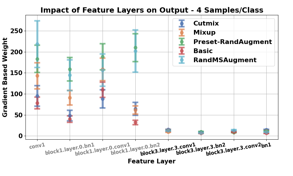
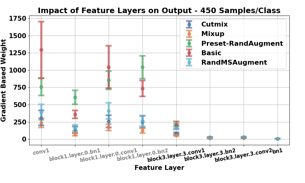
(a)	(b)
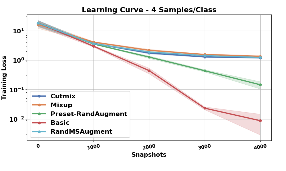
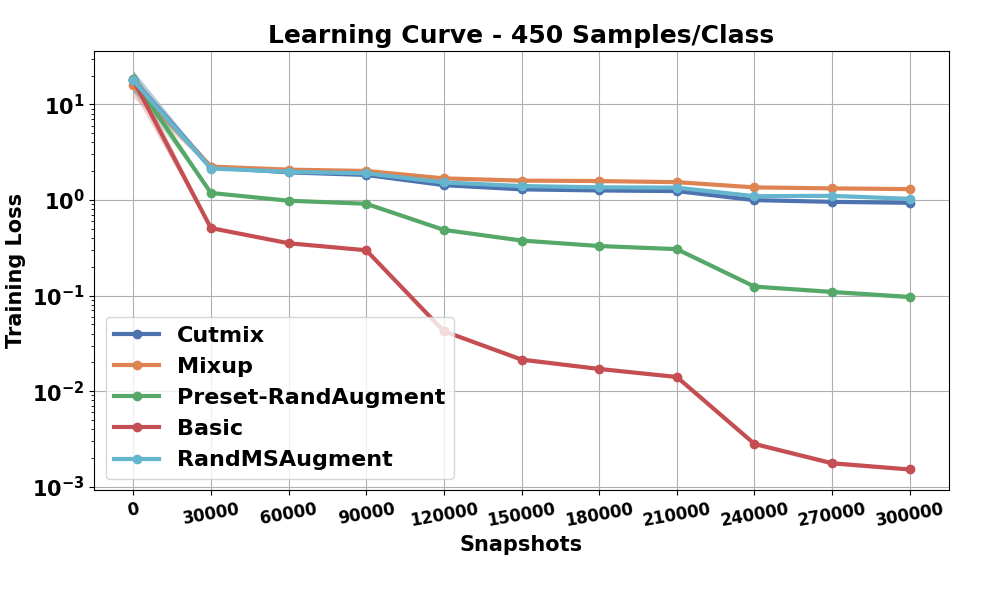
(c)	(d)

Figure 8: (a-b) Gradient based weights $w_{r}^{c}$ averaged over all samples $(\mathbf{x},\mathbf{y})\in\mathcal{V}_{e}$, for 4 lowest (gray) and highest (black) feature maps in the model. The weights for RandMSAugment is especially high for sparse labels. (c-d) Learning curve for different augmentation methods is shown, where RandMSAugment’s convergence speed is closer to MSDA methods. Averages are computed over 3 models trained with different random seeds.

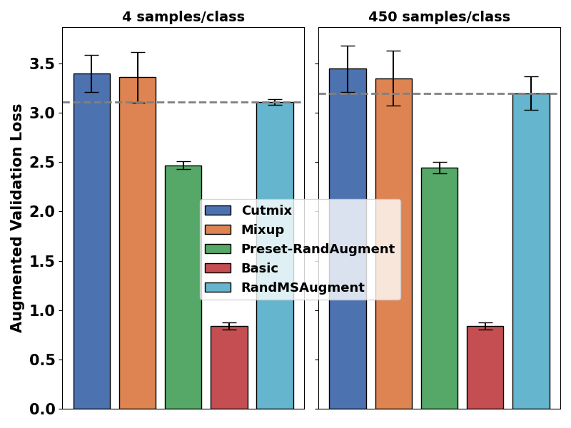
Figure 9: Distributional similarity of RandMSAugment samples to $P_{e}$, compared to samples from different augmentations. The realism is RandMSAugment samples is between Preset-RandAugment and MSDA methods. Error bars are computed over 3 models trained with different random seeds.

7.5 Ablation Study with Parameter $\alpha$

Next, we empirically analyse the parameter $\alpha$ that is used to modify the shape of the Beta distribution, from which the interpolation parameter $\lambda$ is drawn. When $\alpha<1$, the distribution is skewed towards 0, whereas $\alpha=1$ produces a uniform distribution. We compare the performance of Mixup and RandMSAugment for two values of the parameter $\alpha$ recommended in [48] in Table 11. The differences in the performance between the two cases does not seem to be statistically significant.

Augmentation	Samples / Class
	4	25	100	500
Mixup $\alpha=0.2$	5.39$\pm$3.52	27.30$\pm$0.46	47.91$\pm$0.24	66.02$\pm$0.25
Mixup $\alpha=1.0$	7.79$\pm$0.19	25.18$\pm$0.30	45.85$\pm$0.69	65.89$\pm$0.17
RandMSAugment $\alpha=0.2$	14.48$\pm$0.27	34.61$\pm$0.23	52.37$\pm$0.08	69.96$\pm$0.27
RandMSAugment $\alpha=1.0$	13.12$\pm$0.47	33.90$\pm$0.35	52.22$\pm$0.16	70.64$\pm$0.16

Table 11: Comparison between results obtained with $\alpha=0.2$ and $\alpha=1.0$ for Mixup and RandMSAugment in terms of Top-1 accuracy (%, $\uparrow$) on Tiny-Imagenet. In most cases, the standard error across corresponding results overlaps and is therefore not statistically significant. We use $\alpha=0.2$ in our main experiments as recommended by the Mixup paper [48] for Tiny-Imagenet, which seems to work better overall with both Mixup and RandMSAugment.

7.6 Ablation Study with Different Learning Rates

Finally, we show that the difference between results obtained with slightly different training settings is small. Some methods [24] use a learning rate of 0.1 to train Tiny-Imagenet. Table 12 shows that the difference in performance between using a learning rate of 0.1 and 0.03 on Tiny-Imagenet is under 1% in most cases, and that a learning rate of 0.03 does best overall.

Augmentation	Samples / Class
	4	25	100	500
Preset-RandAugment $lr=0.1$	11.63$\pm$0.16	32.62$\pm$0.03	49.05$\pm$0.05	66.59$\pm$0.30
Preset-RandAugment $lr=0.03$	10.54$\pm$0.13	29.43$\pm$0.10	49.20$\pm$0.15	67.47$\pm$0.10
ResizeMix $lr=0.1$	8.53$\pm$0.05	24.16$\pm$0.12	45.97$\pm$0.04	66.56$\pm$0.43
ResizeMix $lr=0.03$	7.80$\pm$0.10	25.69$\pm$0.13	46.06$\pm$0.57	67.77$\pm$0.22
Mixup $lr=0.1$	7.79$\pm$0.11	25.38$\pm$0.64	44.30$\pm$0.03	65.52$\pm$0.08
Mixup $lr=0.03$	7.92$\pm$0.16	27.30$\pm$0.46	47.91$\pm$0.24	66.02$\pm$0.25
RandMSAugment $lr=0.1$	14.21$\pm$0.00	34.30$\pm$0.34	52.42$\pm$0.41	69.15$\pm$1.36
RandMSAugment $lr=0.03$	14.48$\pm$0.27	34.61$\pm$0.22	52.37$\pm$0.09	69.96$\pm$0.27

Table 12: Comparison between the Top-1 accuracies (%, $\uparrow$) obtained with using a learning rate of 0.1 and 0.03 to train Tiny-Imagenet. $lr=0.03$ (second row) does better overall, even while the difference between the two cases is mostly small and under 1%.

7.7 More RandMSAugment Examples

FeatXform, ReszPst
FeatXform, Interp
ReszPst, Interp

Figure 10: More examples from RandMSAugment.

References

- Baek et al. [2021] Kyungjune Baek, Duhyeon Bang, and Hyunjung Shim. Gridmix: Strong regularization through local context mapping. Pattern Recognition, 109:107594, 2021.
- Bengio et al. [2009] Yoshua Bengio, Jérôme Louradour, Ronan Collobert, and Jason Weston. Curriculum learning. In Proceedings of the 26th annual international conference on machine learning, pages 41–48, 2009.
- Berthelot et al. [2019] David Berthelot, Nicholas Carlini, Ekin D Cubuk, Alex Kurakin, Kihyuk Sohn, Han Zhang, and Colin Raffel. Remixmatch: Semi-supervised learning with distribution alignment and augmentation anchoring. arXiv preprint arXiv:1911.09785, 2019.
- Chapelle et al. [2000] Olivier Chapelle, Jason Weston, Léon Bottou, and Vladimir Vapnik. Vicinal risk minimization. Advances in neural information processing systems, 13, 2000.
- Cheung and Yeung [2022] Tsz-Him Cheung and Dit-Yan Yeung. Transformmix: Learning transformation and mixing strategies for sample-mixing data augmentation. 2022.
- Chidambaram et al. [2021] Muthu Chidambaram, Xiang Wang, Yuzheng Hu, Chenwei Wu, and Rong Ge. Towards understanding the data dependency of mixup-style training. arXiv preprint arXiv:2110.07647, 2021.
- Chrabaszcz et al. [2017] Patryk Chrabaszcz, Ilya Loshchilov, and Frank Hutter. A downsampled variant of imagenet as an alternative to the cifar datasets. arXiv preprint arXiv:1707.08819, 2017.
- Coates et al. [2011] Adam Coates, Andrew Ng, and Honglak Lee. An analysis of single-layer networks in unsupervised feature learning. In Proceedings of the fourteenth international conference on artificial intelligence and statistics, pages 215–223. JMLR Workshop and Conference Proceedings, 2011.
- Cubuk et al. [2019] Ekin D. Cubuk, Barret Zoph, Dandelion Mane, Vijay Vasudevan, and Quoc V. Le. Autoaugment: Learning augmentation strategies from data. In Proceedings of the IEEE/CVF Conference on Computer Vision and Pattern Recognition (CVPR), 2019.
- Cubuk et al. [2020] Ekin D Cubuk, Barret Zoph, Jonathon Shlens, and Quoc V Le. Randaugment: Practical automated data augmentation with a reduced search space. In Proceedings of the IEEE/CVF conference on computer vision and pattern recognition workshops, pages 702–703, 2020.
- Cubuk et al. [2021] Ekin Dogus Cubuk, Ethan S Dyer, Rapha Gontijo Lopes, and Sylvia Smullin. Tradeoffs in data augmentation: An empirical study. 2021.
- Dabouei et al. [2021] Ali Dabouei, Sobhan Soleymani, Fariborz Taherkhani, and Nasser M Nasrabadi. Supermix: Supervising the mixing data augmentation. In Proceedings of the IEEE/CVF conference on computer vision and pattern recognition, pages 13794–13803, 2021.
- Dalal and Triggs [2005] Navneet Dalal and Bill Triggs. Histograms of oriented gradients for human detection. In 2005 IEEE computer society conference on computer vision and pattern recognition (CVPR’05), pages 886–893. Ieee, 2005.
- DeVries and Taylor [2017] Terrance DeVries and Graham W Taylor. Improved regularization of convolutional neural networks with cutout. arXiv preprint arXiv:1708.04552, 2017.
- Facciolo et al. [2017] Gabriele Facciolo, Carlo De Franchis, and Enric Meinhardt-Llopis. Automatic 3d reconstruction from multi-date satellite images. In Proceedings of the IEEE Conference on Computer Vision and Pattern Recognition Workshops, pages 57–66, 2017.
- Geiping et al. [2022] Jonas Geiping, Micah Goldblum, Gowthami Somepalli, Ravid Shwartz-Ziv, Tom Goldstein, and Andrew Gordon Wilson. How much data are augmentations worth? an investigation into scaling laws, invariance, and implicit regularization. arXiv preprint arXiv:2210.06441, 2022.
- Goodfellow et al. [2016] Ian Goodfellow, Yoshua Bengio, and Aaron Courville. Deep learning. MIT press, 2016.
- Harris et al. [2020] Ethan Harris, Antonia Marcu, Matthew Painter, Mahesan Niranjan, Adam Prügel-Bennett, and Jonathon Hare. Fmix: Enhancing mixed sample data augmentation. arXiv preprint arXiv:2002.12047, 2020.
- He et al. [2016] Kaiming He, Xiangyu Zhang, Shaoqing Ren, and Jian Sun. Identity mappings in deep residual networks. In Computer Vision–ECCV 2016: 14th European Conference, Amsterdam, The Netherlands, October 11–14, 2016, Proceedings, Part IV 14, pages 630–645. Springer, 2016.
- Hendrycks et al. [2019] Dan Hendrycks, Norman Mu, Ekin D Cubuk, Barret Zoph, Justin Gilmer, and Balaji Lakshminarayanan. Augmix: A simple data processing method to improve robustness and uncertainty. arXiv preprint arXiv:1912.02781, 2019.
- Ho et al. [2019] Daniel Ho, Eric Liang, Xi Chen, Ion Stoica, and Pieter Abbeel. Population based augmentation: Efficient learning of augmentation policy schedules. In International Conference on Machine Learning, pages 2731–2741. PMLR, 2019.
- Huang et al. [2021] Shaoli Huang, Xinchao Wang, and Dacheng Tao. Snapmix: Semantically proportional mixing for augmenting fine-grained data. In Proceedings of the AAAI Conference on Artificial Intelligence, pages 1628–1636, 2021.
- Kang and Kim [2023] Minsoo Kang and Suhyun Kim. Guidedmixup: an efficient mixup strategy guided by saliency maps. In Proceedings of the AAAI Conference on Artificial Intelligence, pages 1096–1104, 2023.
- Kim et al. [2020] Jang-Hyun Kim, Wonho Choo, and Hyun Oh Song. Puzzle mix: Exploiting saliency and local statistics for optimal mixup. In International Conference on Machine Learning, pages 5275–5285. PMLR, 2020.
- Kim et al. [2021] Jang-Hyun Kim, Wonho Choo, Hosan Jeong, and Hyun Oh Song. Co-mixup: Saliency guided joint mixup with supermodular diversity. arXiv preprint arXiv:2102.03065, 2021.
- Krizhevsky et al. [2009] Alex Krizhevsky, Geoffrey Hinton, et al. Learning multiple layers of features from tiny images. 2009.
- Krizhevsky et al. [2012] Alex Krizhevsky, Ilya Sutskever, and Geoffrey E Hinton. Imagenet classification with deep convolutional neural networks. Advances in neural information processing systems, 25, 2012.
- Li et al. [2021] Boyi Li, Felix Wu, Ser-Nam Lim, Serge Belongie, and Kilian Q Weinberger. On feature normalization and data augmentation. In Proceedings of the IEEE/CVF conference on computer vision and pattern recognition, pages 12383–12392, 2021.
- Lim et al. [2019] Sungbin Lim, Ildoo Kim, Taesup Kim, Chiheon Kim, and Sungwoong Kim. Fast autoaugment. Advances in Neural Information Processing Systems, 32, 2019.
- Lowe [2004] G Lowe. Sift-the scale invariant feature transform. Int. J, 2(91-110):2, 2004.
- Marcu and Prugel-Bennett [2022] Antonia Marcu and Adam Prugel-Bennett. On the effects of artificial data modification. In International Conference on Machine Learning, pages 15050–15069. PMLR, 2022.
- Oh and Yun [2023] Junsoo Oh and Chulhee Yun. Provable benefit of mixup for finding optimal decision boundaries. In International Conference on Machine Learning, pages 26403–26450. PMLR, 2023.
- Oliver et al. [2018] Avital Oliver, Augustus Odena, Colin A Raffel, Ekin Dogus Cubuk, and Ian Goodfellow. Realistic evaluation of deep semi-supervised learning algorithms. Advances in neural information processing systems, 31, 2018.
- Park et al. [2022] Chanwoo Park, Sangdoo Yun, and Sanghyuk Chun. A unified analysis of mixed sample data augmentation: A loss function perspective. Advances in Neural Information Processing Systems, 35:35504–35518, 2022.
- Pinto et al. [2022] Francesco Pinto, Harry Yang, Ser Nam Lim, Philip Torr, and Puneet Dokania. Using mixup as a regularizer can surprisingly improve accuracy & out-of-distribution robustness. Advances in Neural Information Processing Systems, 35:14608–14622, 2022.
- Qin et al. [2020] Jie Qin, Jiemin Fang, Qian Zhang, Wenyu Liu, Xingang Wang, and Xinggang Wang. Resizemix: Mixing data with preserved object information and true labels. arXiv preprint arXiv:2012.11101, 2020.
- Selvaraju et al. [2017] Ramprasaath R Selvaraju, Michael Cogswell, Abhishek Das, Ramakrishna Vedantam, Devi Parikh, and Dhruv Batra. Grad-cam: Visual explanations from deep networks via gradient-based localization. In Proceedings of the IEEE international conference on computer vision, pages 618–626, 2017.
- Simonyan et al. [2013] Karen Simonyan, Andrea Vedaldi, and Andrew Zisserman. Deep inside convolutional networks: Visualising image classification models and saliency maps. arXiv preprint arXiv:1312.6034, 2013.
- Sohn et al. [2020] Kihyuk Sohn, David Berthelot, Nicholas Carlini, Zizhao Zhang, Han Zhang, Colin A Raffel, Ekin Dogus Cubuk, Alexey Kurakin, and Chun-Liang Li. Fixmatch: Simplifying semi-supervised learning with consistency and confidence. Advances in neural information processing systems, 33:596–608, 2020.
- Uddin et al. [2020] AFM Uddin, Mst Monira, Wheemyung Shin, TaeChoong Chung, Sung-Ho Bae, et al. Saliencymix: A saliency guided data augmentation strategy for better regularization. arXiv preprint arXiv:2006.01791, 2020.
- Van der Maaten and Hinton [2008] Laurens Van der Maaten and Geoffrey Hinton. Visualizing data using t-sne. Journal of machine learning research, 9(11), 2008.
- Verma et al. [2019] Vikas Verma, Alex Lamb, Christopher Beckham, Amir Najafi, Ioannis Mitliagkas, David Lopez-Paz, and Yoshua Bengio. Manifold mixup: Better representations by interpolating hidden states. In International conference on machine learning, pages 6438–6447. PMLR, 2019.
- Wold et al. [1987] Svante Wold, Kim Esbensen, and Paul Geladi. Principal component analysis. Chemometrics and intelligent laboratory systems, 2(1-3):37–52, 1987.
- Xie et al. [2020] Qizhe Xie, Zihang Dai, Eduard Hovy, Thang Luong, and Quoc Le. Unsupervised data augmentation for consistency training. Advances in neural information processing systems, 33:6256–6268, 2020.
- Yun et al. [2019] Sangdoo Yun, Dongyoon Han, Seong Joon Oh, Sanghyuk Chun, Junsuk Choe, and Youngjoon Yoo. Cutmix: Regularization strategy to train strong classifiers with localizable features. In Proceedings of the IEEE/CVF international conference on computer vision, pages 6023–6032, 2019.
- Zagoruyko and Komodakis [2016] Sergey Zagoruyko and Nikos Komodakis. Wide residual networks. arXiv preprint arXiv:1605.07146, 2016.
- Zhang et al. [2021] Bowen Zhang, Yidong Wang, Wenxin Hou, Hao Wu, Jindong Wang, Manabu Okumura, and Takahiro Shinozaki. Flexmatch: Boosting semi-supervised learning with curriculum pseudo labeling. Advances in Neural Information Processing Systems, 34:18408–18419, 2021.
- Zhang et al. [2017] Hongyi Zhang, Moustapha Cisse, Yann N Dauphin, and David Lopez-Paz. mixup: Beyond empirical risk minimization. arXiv preprint arXiv:1710.09412, 2017.
- Zhang et al. [2020] Linjun Zhang, Zhun Deng, Kenji Kawaguchi, Amirata Ghorbani, and James Zou. How does mixup help with robustness and generalization? arXiv preprint arXiv:2010.04819, 2020.
- Zhong et al. [2020] Zhun Zhong, Liang Zheng, Guoliang Kang, Shaozi Li, and Yi Yang. Random erasing data augmentation. In Proceedings of the AAAI conference on artificial intelligence, pages 13001–13008, 2020.
- Zhou et al. [2020] Tianyi Zhou, Shengjie Wang, and Jeff Bilmes. Time-consistent self-supervision for semi-supervised learning. In Proceedings of the 37th International Conference on Machine Learning, pages 11523–11533. PMLR, 2020.
- Zhu et al. [2020] Jianchao Zhu, Liangliang Shi, Junchi Yan, and Hongyuan Zha. Automix: Mixup networks for sample interpolation via cooperative barycenter learning. In Computer Vision–ECCV 2020: 16th European Conference, Glasgow, UK, August 23–28, 2020, Proceedings, Part X 16, pages 633–649. Springer, 2020.