Exploring Straighter Trajectories of Flow Matching with Diffusion Guidance

Abstract

Flow matching as a paradigm of generative model achieves notable success across various domains. However, existing methods use either multi-round training or knowledge within minibatches, posing challenges in finding a favorable coupling strategy for straight trajectories. To address this issue, we propose a novel approach, Straighter trajectories of Flow Matching (StraightFM). It straightens trajectories with the coupling strategy guided by diffusion model from entire distribution level. First, we propose a coupling strategy to straighten trajectories, creating couplings between image and noise samples under diffusion model guidance. Second, StraightFM also integrates real data to enhance training, employing a neural network to parameterize another coupling process from images to noise samples. StraightFM is jointly optimized with couplings from above two mutually complementary directions, resulting in straighter trajectories and enabling both one-step and few-step generation. Extensive experiments demonstrate that StraightFM yields high quality samples with fewer step. StraightFM generates visually appealing images with a lower FID among diffusion and traditional flow matching methods within 5 sampling steps when trained on pixel space. In the latent space (i.e., Latent Diffusion), StraightFM achieves a lower KID value compared to existing methods on the CelebA-HQ 256 dataset in fewer than 10 sampling steps.

1 Introduction

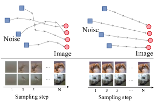
(a) Flow matching

((a))

(b) Ours

((b))

Figure 1: Illustration about flow matching with independent couplings and ours. SraightFM (top-right) supports straighter trajectories than Flow matching with independent couplings (top-left), thus generating high-quality images with fewer steps (bottom).

Generative models have achieved remarkable success across multiple fields. One large class of generative models builds a mapping from data distribution to the prior distribution and learns the inverse mapping with ordinary differential equation (ODE) to generate data. Using this paradigm, diffusion models have made significant progress in various domains [40, 42, 14, 6, 32, 37, 4]. Notably, an emerging type of approach, known as flow matching [29, 27, 1], can achieve one-step generation while perform comparably with the diffusion models [29, 25, 49]. Flow matching methods estimate a time-dependent velocity field (i.e., the drift term of ODE) similar to the diffusion models but sidestep the subtle selection of hyper-parameters. As depicted in Fig. 1, flow matching methods first identify a coupling strategy that binds elements in prior distribution to those in data distribution when calculating objectives to learn the shortest straight path between each coupling [29, 30]. With nearly straight trajectories, flow matching methods can facilitate one-step generation with Euler method while performing comparably with diffusion models.

Discovering tractable and scalable sample couplings for flow matching remains a challenging problem. The ideal solution of a coupling strategy would be an optimal transport plan, but this is computationally prohibitive for high-dimensional data. Thus, existing flow matching methods typically fall into two types to yield effective couplings for straightening path: multi-round straightening training [29] and leveraging underlying information within minibatches [36, 45, 46]. Specifically, Rectified Flow (RF) [29] gradually finds effective couplings by recursively training a new RF with synthesized data from the previous one. Nevertheless, the multi-round training strategy raises concerns about the degradation in image quality or diversity [2]. On the other hand, concurrent works leverage inherent information over samples to derive couplings [46, 36], i.e., solving the optimal transport (OT) problem within minibatch samples. However, minibatch samples does not capture the complexity across the whole data distribution, hindering the applications of these methods to real-world tasks.

In this work, we explore a novel solution: finding scalable and tractable couplings for flow matching with the guidance of diffusion model. We take inspiration from the recent works that use pre-trained diffusion models to train a new one with improved sample quality and inference speed [38, 33, 43]. Although flow matching and Probability Flow Ordinary Differential Equation (PF-ODE) of diffusion models adopt independent training tactics, they share similar principles: First, both methods construct time-dependent ODEs to map between two distributions. Second, recent literature [8, 23, 29] has highlighted that diffusion and flow matching models minimize either the Wasserstein distance or a generalized transport cost. Moreover, since well-trained diffusion models have learned the entire data distribution, we can obtain non-trivial couplings with the assistance of diffusion and thus skip the procedure of solving OT problems on minibatches.

Our work explores Straighter trajectories of Flow Matching with diffusion model guidance (StraightFM). Specifically, we utilize a well-trained diffusion model to synthesize pseudo-data. The pair of one pseudo-image and its corresponding initial noise constitutes a coupling provided to flow matching. Similar to most flow matching methods, StraightFM employs a time-independent model to match the drift term of one ODE, which is a velocity field pointing to the direction of the shortest straight path between each coupling. We subsequently set the intermediate sample state as a linear interpolation of each coupling along this shortest straight path. To straighten trajectory, the training objective of flow matching guides this time-independent model at each intermediate state to match the velocity field with a simple unconstrained least squares objective function.

In addition, StraightFM fully utilizes two directions of the coupling process to improve the training of flow matching by further incorporating real samples to form effective couplings. As discussed above, the first direction involves transitioning from noise to image samples, under the guidance of a diffusion model. The second direction is pointing image to noise samples, employing a neural network to parameterize this process. Subsequently, we integrate the KL divergence to impose the distribution of this neural network to approximate the original noise distribution. The comprehensive loss function of straightFM comprises three terms: two direction flow matching objectives to complement each other, and an additional KL term to ensure the validity of couplings from real to noise samples. Benefiting from these two complementary coupling directions, one StraightFM model is capable of achieving one-step and few-step generation with straighter trajectories, in contrast to the multi-round training of RF burdening a sequence of models.

We conducted extensive experiments to assess the effectiveness of StraightFM. With plain hyperparameters, our method can generate high-quality images in the pixel space and be effective for flow matching in the latent space of pre-trained large-scale generative models. In direct pixel-level training, experiments on CIFAR-10 demonstrate that StraightFM significantly achieves straighter paths in few-step and one-step generation, compared with state-of-the-art diffusion and flow matching models. For StraighFM trained on latent space, our experiments outperform the latent diffusion model on CelebA-HQ 256$\times$ 256 dataset within 10 sampling steps. Finally, we apply flow matching to the image restoration task, such as inpainting, showcasing the potential of natural optimal transport couplings to flow matching. The main contributions of this work are summarized as follows:

• We propose a novel coupling strategy for straightening the trajectories of flow matching with diffusion model guidance, bypassing the need for solving OT couplings in minibatch or multi-round training.

• StraightFM further incorporates real samples to construct effective couplings. Thus, one flow matching model is optimized from two mutual complementary directions jointly to facilitate training.

• Extensive experiments demonstrate that StraightFM can generate high-quality image samples in fewer steps, and even one-step generation with straighter trajectories.

2 Related Work

2.1 Generative Model with ODE

Continuous Normalizing Flow aims to model a complex data distribution by transforming a simple distribution through a series of invertible mappings specified by neural ODEs [7]. Training CNF can be categorized into simulation-based and simulation-free methods. Original CNF employs the maximum likelihood objective, which leads to prohibitively expensive ODE simulations during both forward and backward propagation [7, 11]. In contrast, simulation-free methods aim to speed up CNF training by defining the target probability path without the need for ODE simulations. PF-ODE of diffusion [42, 41] presents a particular instance of simulation-free methods. It is trained with a noise conditional score matching objective to estimate the probability distribution, indirectly defining the trajectory. Flow matching, another simulation-free method, demonstrates that the CNF can be trained using a straightforward regression to match vector fields, thus eliminating the need for cumbersome hyperparameter selection.

2.2 Flow Matching Method

Original flow matching relies on independent data and noise pairs when calculating training objectives  [27, 29, 1, 9]. Recent works focus on the coupling strategies between data and noise samples to straighten trajectories and reduce sampling steps. For instance, Optimal Transport Conditional Flow Matching (OT-CFM) [46] performs OT for each batch of data to obtain the permutation matrix for couplings. This strategy was also proposed in  [36] concurrently. Finding couplings within minibatches confines its application to large-scale distribution. It is noted that we classify Rectified Flow [29] as a flow matching method since RF is a specific variant of flow matching with only a slight difference on the noise scheduler. To find effective couplings, RF relies on multi-round training. However, according to the latest discovery [2], training the next generative model using synthesized data from the previous one iteratively leads to the quality degradation of generated samples. Unlike present methods struggling with solving OT problems or multi-round straightening, the coupling strategy of StraightFM generalizes the range of coupling approaches with the guidance of diffusion model to few-step and one-step generation.

2.3 Diffusion Model

Recent diffusion model achieves impressive performance in image generation. Prior works group the sampling procedure of diffusion models into two categories: training-free and training-based methods. Training free methods, i.e. discretizing stochastic differential equations [14, 42, 3, 17] or PF-ODE of diffusion [41, 28, 31, 52, 54], is a iterative sampling process, which needs 25 to 1000 steps gradually remove the noise from Gaussian random variables to obtain image. Training-based methods rely on extensive training, such as distilling [33, 38], learning variances [3, 34] and combining diffusion with GANs [50], which can notably enhance the sampling speed compared to training-free methods. Existing distillation-based methods are assisted with one well-trained diffusion model, which can notably enhance sample quality and sampling speed of diffusion.

With the well-trained diffusion model guidance, our approach provides another promising direction to achieve one-step generation in only one round of training, sidestepping the potential risk of many rounds of iterations and the intractability issues of OT-CFM in large-scale datasets.

3 Preliminaries

This section defines all foundational concepts of flow matching and diffusion models to present StraightFM.

3.1 Probability Flow ODE of Diffusion Model

A notable property of diffusion models is a deterministic ODE, namely probability flow ODE (PF-ODE), whose trajectory mirrors the marginal probability densities of stochastic diffusion models. Considering samples $\mathbf{x}$ from $d$-dimensional Euclidean space $\mathbb{R}^{d}$ and the intermediate sample at state $t$ as $\mathbf{x}_{t}$, the probability density function of $\mathbf{x}_{t}$, given by $p_{t}(x):[0,1]\times\mathbb{R}^{d}\to\mathbb{R}^{+}$, characterizes the time-varying distribution of $\mathbf{x}_{t}$. The PF-ODE is formulated as follows:

$$\mathrm{d}\mathbf{x}_{t}=\left[\boldsymbol{\mu}\left(\mathbf{x}_{t},t\right)-\frac{1}{2}g(t)^{2}\nabla\log p_{t}\left(\mathbf{x}_{t}\right)\right]\mathrm{d}t,$$ (1)

where $\mu(\cdot,\cdot)$ and $g(\cdot)$ are the drift and diffusion terms of diffusion model, respectively. Typically, diffusion models employ a time-dependent model to approximate $\nabla\log p_{t}\left(\mathbf{x}_{t}\right)$, subsequently generate samples from initial noise by solving Eq. 1 with various numerical ODE solvers, such as Euler method, and Heun’s 2nd order method.

3.2 Flow Matching

Suppose that noise sample $\mathbf{x}_{0}$ from a Gaussian distribution $p_{0}$ and $\mathbf{x}_{1}$ from a data distribution $p_{1}$ over $d$-dimensional Euclidean space $\mathbb{R}^{d}$, flow matching defines a time-independent ordinary differential equation:

$$\mathrm{d}\mathbf{x}_{t}=v(\mathbf{x}_{t},t)\mathrm{d}t,t\in[0,1],$$ (2)

where $v:[0,1]\times\mathbb{R}^{d}\to\mathbb{R}^{d}$ represents a vector field.

The primary goal of flow matching is to utilize a velocity model $u_{\theta}$, parameterized by $\theta$, i.e., a time-dependent neural network, to approximate $v$. This is notably intractable for general unknown and complex distributions $p_{t}$. Practically, a simplified objective of conditional flow matching [27, 45, 46] effectively bypasses $v(\cdot)$ by incorporating a latent condition $\mathbf{z}$:

$$\min_{\theta}\mathbb{E}_{t,q(\mathbf{z}),p_{t}(\mathbf{x}|\mathbf{z})}\|u_{\theta}(\mathbf{x}_{t};t)-v_{t}(\mathbf{x}_{t}|\mathbf{z})\|^{2},$$ (3)

which is proved to be equivalent to the objective of flow matching concerning the gradient of model parameters. Usually, $\mathbf{z}$ is identified as a random pair $(\mathbf{x}_{0},\mathbf{x}_{1})$. However, solely relying upon this independent coupling strategy falls short in one step generation [29] and current coupling strategy of existing methods either faces scalability challenges due to the need to solve optimal transport problems within a batch or suffers from a potential risk in the degradation of quality and diversity due to multi-round training.

In this paper, we resolve this shortcoming, proposing a coupling strategy across two distributions to yield high-quality images with fewer steps and straighter trajectories, skipping additionally straightening procedure.

Algorithm 1 Straight Flow Matching

Input: $u_{\theta}$: an initial velocity model with parameter $\theta$, $\psi$: a well-trained diffusion model, $q_{\phi}(\tilde{\mathbf{x}}_{0}|\mathbf{x}_{1})$: a neural network with image $\mathbf{x}_{1}$ as input.
repeat
1. Sample $\mathbf{x}_{0}\sim p_{0}$, $\mathbf{x}_{1}\sim p_{1}$ and $t\sim\text{Uniform}[0,1]$.
2. Sample $\tilde{\mathbf{x}}_{1}$ from the PF-ODE trajectories of diffusion model $\psi$ with $\mathbf{x}_{0}$ as the initial point.
3. Sample $\tilde{\mathbf{x}}_{0}$ from $q_{\phi}(\tilde{\mathbf{x}}_{0}|\mathbf{x}_{1})$ given image $\mathbf{x}_{1}$.
4. Compute the objective $\mathcal{L}$ as in Eq. 7
5. Update $u_{\theta}$ and $q_{\phi}$ by descending gradient of $\mathcal{L}$.
until convergence
Return: $u_{\theta}$: a well-trained velocity model that generates samples from $\mathrm{d}\mathbf{x}_{t}=u_{\theta}(\mathbf{x}_{t},t)\mathrm{d}t$ starting with $\mathbf{x}_{0}\sim p_{0}$.

4 Straight Flow Matching

Identifying effective couplings between image and source samples is key to the success of previous methods. We suggest expanding the scope of current coupling strategies by leveraging the guidance from diffusion models and incorporating real samples to construct couplings. StraightFM is detailed in Algorithm 1.

4.1 Diffusion Model Guidance

Our goal is to build straight trajectories for flow matching with coupling guidance across two distributions to facilitate training and shorten sampling steps. The ideal scenario is searching couplings based on the optimal transport plan over two distribution, but it is prohibitively expensive. Fortunately, due to the underlying connection between flow matching and PF-ODE of diffusion models, as we discussed above, one can use couplings provided by diffusion models to improve flow matching.

Specifically, utilizing a well-trained diffusion model, we can generate one coupling $(\mathbf{x}_{0},\tilde{\mathbf{x}}_{1})$, by starting with an initial noise sample $\mathbf{x}_{0}\sim p_{0}$. Subsequently, $\tilde{\mathbf{x}}_{1}$ is sampled with one numerical ODE solver along the PF-ODE trajectories of a diffusion model according to Eq. 1. After that, the coupling of noise and image samples $(\mathbf{x}_{0},\tilde{\mathbf{x}}_{1})$ is provided to optimize the subsequent objective:

$$\mathcal{L}_{\text{revs}}(u_{\theta},\mathbf{x}_{0},\tilde{\mathbf{x}}_{1})$$ (4)

$$=\mathbb{E}_{t,\mathbf{x}_{0},\tilde{\mathbf{x}}_{1}}\|u_{\theta}(\mathbf{x}_{t};t)-(\tilde{\mathbf{x}}_{1}-\mathbf{x}_{0})\|^{2},$$

where noise sample $\mathbf{x}_{0}$ serves as the initial point for sampling a pseudo-image $\tilde{\mathbf{x}}_{1}$ from the PF-ODE of diffusion model and intermediate state $\mathbf{x}_{t}=t\tilde{\mathbf{x}}_{1}+(1-t)\mathbf{x}_{0},\text{ for all }t\in[0,1]$. Since the coupling process is constructed from the reverse diffusion process, i.e., from noise to image sample, we use the shorthand notion $\mathcal{L}_{\text{revs}}(u_{\theta},\mathbf{x}_{0},\tilde{\mathbf{x}}_{1})$ for  LABEL:eq5.

Intuitively, the objective sets $(\tilde{\mathbf{x}}_{1}-\mathbf{x}_{0})$ as the target velocity field $v$ in Eq. 2, representing the shortest straight path from noise to synthesized samples. And the linear interpolation $\mathbf{x}_{t}$ can be formulated as the intermediate state at $t$ along this shortest path. Following this, LABEL:eq5 is derived by plugging target velocity field $(\tilde{\mathbf{x}}_{1}-\mathbf{x}_{0})$ into Eq. 3.

Using samples generated by diffusion is appropriate due to the remarkable image quality achieved by contemporary diffusion models [17, 37], which closely approximates real images. Moreover, the coupling formed by diffusion is also the approximation of optimal transport [21], which coincides with flow matching [29, 27]. In contrast to Rectified Flow (RF), where training data for $k+1$-RF is derived by synthesizing images from $k$-RF (k$\geq$2), we use synthetic data only one round and are free from multi-round training to generate different couplings, mitigating the potential risk of image quality or diversity decreasing [2]. Subsequent experiments in Sec. 5.1 will further demonstrate that this coupling strategy with one round of training enables one-step and few-step generation.

4.2 Empower with Real Samples

On a parallel track, we also integrate real data $\mathbf{x}_{1}\sim p_{1}$ to find effective couplings. Then the coupling process of StraightFM is derived from two directions, where one is from noise to image, and another is from image to noise, mutually complementing each other for flow matching.

One key difficulty arising when introducing real samples is how to effectively couple them with noise samples in the training of flow matching. A recent work [26] revealed that parameterizing the coupling process with neural networks is more effective than independent coupling to minimize trajectory curvature of ODE-based generative model. Accordingly, we utilize the neural network $q_{\phi}(\tilde{\mathbf{x}}_{0}|\mathbf{x}_{1})p_{1}(\mathbf{x}_{1})$ with parameters $\phi$ to represent the coupling process from real samples to noise samples, where we define $q_{\phi}(\tilde{\mathbf{x}}_{0}|\mathbf{x}_{1})$ is a Gaussian distribution like $p_{0}$. Then, we optimize the following objective to ensure the validity of the coupling ($\tilde{\mathbf{x}}_{0},\mathbf{x}_{1}$):

$$\mathcal{D}_{KL}(q_{\phi}(\tilde{\mathbf{x}}_{0}|\mathbf{x}_{1})\|p_{0})=\frac{1}{2}\sum_{i=1}^{d}(\mu_{(i)}^{2}+\sigma^{2}_{(i)}-\log\sigma^{2}_{(i)}-1).$$ (5)

Here $d$ denotes the dimensionality of samples $\tilde{\mathbf{x}}_{0}$, while $\mu_{(i)}^{2}$ and $\sigma^{2}_{(i)}$ represent the mean and variance of the $(i)$-th component, respectively.

The coupling from image to noise samples is provided to optimize the following objective:

$$\mathcal{L}_{\text{forw}}(u_{\theta},\tilde{\mathbf{x}}_{0},\mathbf{x}_{1})$$ (6)

$$=\mathbb{E}_{t,\tilde{\mathbf{x}}_{0},\mathbf{x}_{1}}\|u_{\theta}(\mathbf{x}_{t};t)-(\mathbf{x}_{1}-\tilde{\mathbf{x}}_{0})\|^{2}.$$

Here, $\mathbf{x}_{t}$ is also denoted as the linear interpolation between the coupling $(\tilde{\mathbf{x}}_{0},\mathbf{x}_{1})$ along the shortest straight path. Corresponding to LABEL:eq5, we denote this objective as $\mathcal{L}_{\text{forw}}$.

Recall that StraightFM is expected to utilize the above two couplings to enhance training, the overall objective of StraightFM is formulated as:

$$\min_{\theta,\phi} \mathcal{L}_{\text{revs}}(u_{\theta},\mathbf{x}_{0},\tilde{\mathbf{x}}_{1})+\lambda\mathcal{D}_{KL}(q_{\phi}(\tilde{\mathbf{x}}_{0}|\mathbf{x}_{1})\|p_{0})$$ (7)

$$+\mathcal{L}_{\text{forw}}(u_{\theta},\tilde{\mathbf{x}}_{0},\mathbf{x}_{1}),$$

where $\lambda$ is a hyperparameters. StraightFM jointly minimizes Eq. 7 to update the parameters of $u_{\theta}$ and $q_{\phi}$ with a fast convergence speed.

After training, one can discretize ODE in Eq. 2 just using N-step Euler method to generate samples as follows:

$$\hat{\mathbf{x}}_{({i}+1)/N}\leftarrow\hat{\mathbf{x}}_{{i}/N}+\frac{1}{N}u_{\theta}\left(\hat{\mathbf{x}}_{{i}/N},\frac{i}{N}\right),i\in\{0,\cdots,N-1\}.$$ (8)

Overall, couplings provided to StraightFM are divided into two groups, i.e., $(\tilde{\mathbf{x}}_{0},{\mathbf{x}}_{1})$ and $(\mathbf{x}_{0},\tilde{\mathbf{x}}_{1})$. Here $(\tilde{\mathbf{x}}_{0},{\mathbf{x}}_{1})$ is derived from the above image to noise process, and $(\mathbf{x}_{0},\tilde{\mathbf{x}}_{1})$ is obtained from the generative process of diffusion model. Attributed to the coupling from two complementary directions, StraightFM can obtain the capabilities of straightening trajectories and one-step generation following Eq. 8. If the coupling process only relies on the direction of real data to noise, the model will struggle with one-step generation [26], which is discussed in Sec. 5.2.1.

5 Experiments

In this section, we first validate the mapping similarity of flow matching and PF-ODE of diffusion models to support our primary motivation, showing a high degree of similarity between two models from numerical measurements and visualization. Then, we assess the performance of StraightFM on CIFAR-10 and CelebA-HQ $256\times 256$ datasets for image generation task. Furthermore, we extend the application of flow matching to the image inpainting task on FFHQ $256\times 256$ dataset, thereby demonstrating the efficacy of coupling strategy during flow matching training.

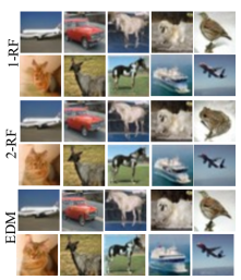
Figure 2: Samples generated by 1-RF with RK45 (top), 2-RF with RK45 (middle) and EDM with Heun 2nd order method (bottom). Corresponding images are generated from the same initial noise.

5.1 Mapping Similarity between FM and Diffusion

This subsection revolves around the discrepancy between samples from flow matching and diffusion models, discovering that the PF-ODE of diffusion map coincides with flow matching. To set up our experiments, we compare flow matching models, 1-RF and 2-RF [29], with diffusion models, VP-ODE [42] and EDM [17]. We measure the differences in 25,600 image-noise pairs sampled from above models with the same initial noise as the input to assess the mapping similarity between the two models.

As depicted in Tab. 1 and Fig. 2, generated images from both models display high similarities in numerical metrics and visual content, regardless of whether it is the earliest diffusion model VP-ODE or current state-of-the-art EDM. A few images show minor differences but still maintain obvious structural similarity. There are notable similarities between the two mappings, despite flow matching and diffusion models being two distinct training tactics, and both models are trained independently. These observations match our prior analysis and motivate our coupling approach with diffusion guidance to enhance flow matching, making it easier to find couplings and generates samples with fewer steps and straighter trajectories. Consequently, we circumvent the need for multi-round training or solving OT problems to obtain different couplings.

Table 1: Comparison of 25,600 noise-image pairs from flow matching and diffusion models with identical inputs on CIFAR-10, measured by MSE and LPIPS. Samples generated from VP-ODE with adaptive RK45 and from EDM with 17 Heun’s 2nd steps [17]. $\downarrow$ means lower is better.

	MSE$\downarrow$		LPIPS$\downarrow$
	VP-ODE [42]	EDM [17]	VP-ODE [42]	EDM [17]
1-RF [29]	0.0065	0.0055	0.21	0.19
2-RF [29]	0.0053	0.0043	0.18	0.15

N=1

N=3

N=5

Ada. N

N=1

N=3

N=5

Ada. N

EDM

1-RF

2-RF

3-RF

Ours-I

Ours-II

Figure 3: Comparison includes diffusion model (EDM), flow matching models (RF) and StraightFM (Ours) trained on CIFAR-10 when simulated with fixed and adaptive steps (N). All corresponding samples are generated from the same initial noise. EDM uses 2nd order Heun method with 17 steps in adaptive sampling.

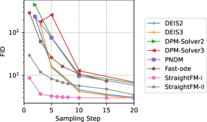
Figure 4: FID performance across different sampling steps on CIFAR-10. Fast-ode, StraightFM-I and StraightFM-II still employ the Euler method for sampling.

5.2 Few-Step Image Generation

For generative task, we employ StraightFM to learn flow matching models on the pixel space of CIFAR-10 [22] and the latent space of an auto-encoder to enhance computational efficiency for high-resolution dataset CelebA-HQ 256$\times$256 [15]. Results are evaluated according to IS (Inception Score [39]), FID (Fréchet Inception Distance [13]) and KID (Kernel Inception Distance [5]). Throughout this subsection, we apply two settings of StraightFM to verify the coupling provided by diffusion models: one without and one integrating real data to find effective couplings, denoted as StraightFM-I and StraightFM-II, respectively. For StraightFM-II, the percentage of couplings from two directions is 50%, and we leave the exploration of different data percentages as future work.

Table 2: Sample quality assessment on CIFAR-10, evaluated using FID-50K. $\uparrow$ means higher is better, and $\downarrow$ means lower is better.

Model Class	Method	IS$\uparrow$	FID$\downarrow$
Optimal Transport	Multi-stage SB [47]	-	12.32
	DOT [44]	-	15.78
RK45	DDPM  [42]	9.37	3.93
Adaptive Step	DDIM (Euler, N=1000) [41]	-	4.04
	1-RectifiedFlow [29]	9.60	2.58
	2-RectifiedFlow [29]	9.24	3.36
	3-RectifiedFlow [29]	9.01	3.96
	FM  [27]	-	6.35
	I-CFM [46]	-	3.66
	OT-CFM [46]	-	3.58
	fast-ode, configA  [26]	9.32	3.37
	fast-ode, configB  [26]	9.55	2.47
	StraightFM-I (Ours)	9.52	2.94
	StraightFM-II (Ours)	9.51	2.82

RF

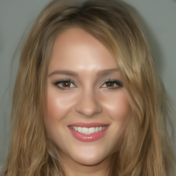
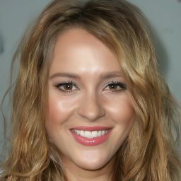
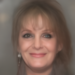
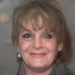
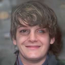
LDM

LFM

Ours-I

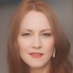
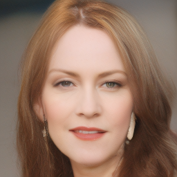
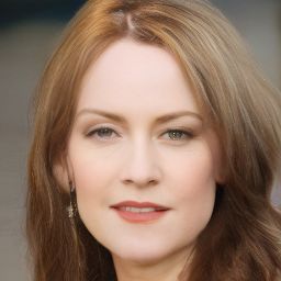
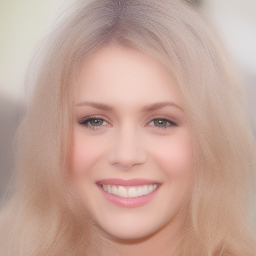
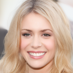
Ours-II

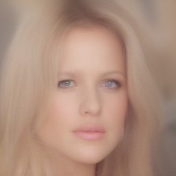
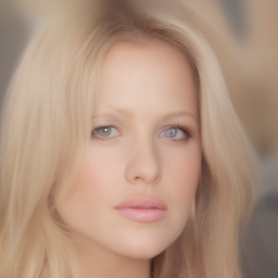
N=5

N=10

N=20

N=5

N=10

N=20

Figure 5: Samples generated on CelebA-HQ $256\times 256$ dataset utilizing varying sampling steps (N). Here, corresponding images from LDM,LFM and StraightFM are initialized from same noise, expect RF, which is trained on the pixel space rather than the latent space.

5.2.1 Image Generation on Pixel Space

Settings. To set up our experiments on CIFAR 10, we consider leveraging diffusion model EDM [17] as the guidance of Straight-FM training. The resolution of the images is set to 32 $\times$ 32. We follow the plain parameters as  [29], which adopts the U-Net of DDPM++ [42]. For the ODE solver, we test the Euler method with limited steps and Runge-Kutta method of order 5(4) with adaptive steps. Further details are available in Supp. 1.1.

Qualitative Comparison. Fig. 3 visually compares images generated from two identical initial noises with limited sampling steps. Our approach consistently produces high-quality images even in on one-step generation, yielding straighter trajectories. Notably, our trajectories are largely independent of the sampling step $N$, in contrast to the generated images of EDM and 1-RF, which are highly sensitive to $N$ (as seen in the 3rd and 4th rows of 1-RF and EDM in Fig. 3). This suggests that our trajectories are more direct than the other models. Moreover, while StraightFM and 1-RF experience single-round training, 1-RF cannot generate images with a single step. Relying on multi-round training, even if 3-RF can achieve single-step generation, the generated images of the 1st to 4th rows show the obvious distinction when changing the sampling step. Although couplings provided by the diffusion model were adopted, the generative results of our method under the same input still differ from those generated by EDM model. This indicates that the model does not simply memorize the training data but truly learns the entire data distribution.

Table 3: Comparison of FID10K and KID10K metrics on on CelebA-HQ 256$\times$ 256 dataset. *Our reimplementation. Bold indicates the best result. Underline indicates the second-best.

	FID$\times 10^{-1}$ $\downarrow$			KID$\times 10$ $\downarrow$
Sampling Step	5	10	20	5	10	20
Rectified Flow	45.71	43.96	40.02	4.66	4.56	4.00
Latent Diffusion	10.71	6.57	3.76	1.07	0.64	0.35
Latent-FM*	8.53	5.82	4.53	0.86	0.59	0.47
StraightFM-I (Ours)	9.17	5.47	3.83	0.87	0.50	0.34
StraightFM-II (Ours)	8.86	5.35	3.78	0.84	0.48	0.33

Quantitative Comparison. As shown in Tab. 2, we first report FID and IS evaluated on the CIFAR-10 dataset from adaptive step sampling. Additionally, Fig. 4 displays FID performance with different sampling steps compared with existing popular diffusion sampler [52, 31, 28]. Specififically, both settings of StraightFM achieve comparable results on FID and IS when simulated with the adaptive step sampling. It is noted that fast-ode [26], which solely relies on the coupling process from image to noise, achieves high-quality image generation with adaptive-step but fails in one-step and few-step generation. When the number of steps is less than 3, FID from StraightFM is nearly an order of magnitude lower than other methods, as visualized in Fig. 4, indicating superior image quality. When the sampling step $N$ increases (greater than 5), the image quality of StraightFM remains comparable among popular diffusion models [14, 42] with fast numerical ODE solvers. The characteristics of StraightFM-I and StraightFM-II can be summarized as follows: StraightFM-I is more independent of the sampling step for few-step generation, while StraightFM-II achieves a better performance in adaptively deciding the sampling step. We suppose that StraightFM gives more consideration to the guidance mechanism from diffusion, when limited on a low-resolution image space.

5.2.2 Image Generation on Latent Space

Settings. Conducting the generative process in the latent space of the generative model [16, 37] provides a different approach to high-resolution image generation with lower computational costs. Thus, we apply StraightFM in the latent space of the pretrained VAE from Latent Diffusion Model (LDM) [37] on CelebA-HQ 256$\times$256, which enhances computational efficiency in high-resolution image synthesis. Additionally, LDM serves as a guide during StraightFM training. We adhere to the baseline parameters used in Latent Flow Matching (LFM, training flow matching in the latent space of LDM) [9]. For coupling sampling, we adopt DDIM sampler, which can be reformulated as a specific instance of PF-ODE [41]. Namely, StraightFM is compared with Rectified Flow (RF) [29], Latent Flow Matching (LFM) [9] and Latent Diffusion Model (LDM) [37] on CelebA-HQ dataset, with all result reported in Tab. 3 and Fig. 5. Further experimental details and results are available in Supp. 1.2.

Results. StraightFM achieves a comparable level of performance on the FID and KID as shown in Tab. 3 with fewer steps, and the samples from StraightFM are largely unaffected by the sampling step, implying more direct trajectories. In Fig. 5, samples from LDM, LFM, and StraightFM use the same initial noise vector, except for RF, which is trained on pixel space. Significantly, at N=5, samples from LFM unexpectedly coincide with ours despite the two models being trained independently from one another. The identity of samples from StraightFM remains consistent across different sampling steps, but samples from LDM and LFM change sharply when the sampling step is less than 10. This suggests that the trajectories of StraightFM are straighter, enabling the generation of higher-quality samples with fewer steps.

Table 4: Inpainting results comparison on three different methods.

	PSNR$\uparrow$	SSIM$\uparrow$	LPIPS $\downarrow$
mGANPrior	23.82	0.71	0.43
SNIPS	30.30	0.65	0.12
Ours	37.43	0.97	0.06

5.3 Image Inpainting

Flow matching methods have been applied in various tasks of image processing, including super-resolution [27] and domain transfer [29] (e.g., from cats to dogs). For image restoration tasks, the pairs of degraded and target images naturally form optimal transport couplings. As a complement to this study, we validate the effectiveness of flow matching in the restoration task, particularly in the inpainting task, addressing the missing parts of images on the FFHQ 256$\times$256 [16] dataset. We mask parts of the original image by randomly dropping 50% of the pixels from 3 channels, respectively. Results are measured by PSNR (Peak Signal-to-Noise Ratio), SSIM (Structural Similarty) [48], and LPIPS (Learned Perceptual Image Patch Similarity) [53]. The exact settings and more comparison are detailed in Supp.1.3.

Fig. 6 shows examples of flow matching in the inpainting task, compared with mGANprior [12] and SNIPS [19], whose degradation configurations are the same as ours. Quantitative results are shown in  Tab. 4. In essence, it demonstrates the potential of an effective coupling strategy, which matches our argument about the significance of coupling strategy in flow-matching performance.

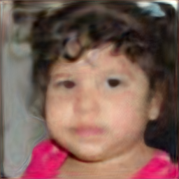
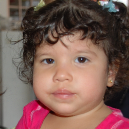
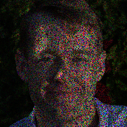
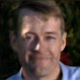
Input

mGANPrior

SNIPS

Ours

Figure 6: Image inpainting examples from different methods on the FFHQ dataset ($256\times 256$).

6 Conclusion

This paper introduces StraightFM, a method that leverages the underlying knowledge from diffusion models to support one-step and few-step generation with straighter trajectories in flow matching. StraightFM also leverages two directions of the coupling process to improve training by incorporating real samples to construct effective couplings, where the two directions of the coupling process complement each other. Empirically, StraightFM produces high-quality results with one sampling step on CIFAR-10 dataset, and visually appealing results within 10 steps on the CelebA-HQ $256\times 256$ dataset, achieving competitive performance in the generative community. In essence, we have explored the high mapping similarity between flow matching and probability flow ODE of diffusion models. As one ODE-based generative model, the distinctive characteristic of StraightFM compared to other available models is the utilization of the underlying information from another independent generative model. This offers exciting prospect to reconsider the connection among various ODE-based generative models.

Supplementary Material

1 Additional Implementation Details

1.1 Implementation Details on the Pixel Space

Our implementation on CIFAR-10 is adapted from the open-source codes of  [42, 17, 29, 26]. In configuring the velocity model $u_{\theta}$ and other hyperparameters, we fully reference the experimental setup used in 1-RectifiedFlow [29] for CIFAR-10, with specific hyperparameters detailed in Tab. 5. For the architecture of $q_{\phi}(\tilde{\mathbf{x}}_{0}|\mathbf{x}_{1})$, we adopt the configuration same as  [26], where $q_{\phi}(\tilde{\mathbf{x}}_{0}|\mathbf{x}_{1})$ is also a smaller UNet than the velocity model. The FID evaluation follows the code of [42]. For StraightFM sampling process, we test two ODE solvers: Euler method for fixed-step sampling and Runge-Kutta method for adaptive-step sampling. The latter employs the relative and absolute tolerances as 1e-5, aligning with the standards of previous studies [42, 29].

1.1.1 Three coupling strategy on CIFAR-10

In the pixel space, our experiments include three strategies, namely StraightFM-I, StraightFM-II, and an additional StraightFM-III, all guided by diffusion models. StraightFM-I and StraightFM-II are similar to those detailed in the body of this paper. For StraightFM-III, we modify the transition process from image to noise. Specifically, we directly leverage the closed form of the forward diffusion process to derive noise from image $\mathbf{x}_{1}$, which is given by:

$$q(\mathbf{x}_{T}|\mathbf{x}_{1})=\mathcal{N}(\mathbf{x}_{T};\sqrt{\bar{\alpha}_{T}}\mathbf{x}_{1},(1-\bar{\alpha}_{T})\mathbf{I}).$$ (1)

The notations $\sqrt{\bar{\alpha}_{T}}$ and $\bar{\alpha}_{T}$ are consistent with their usage in  [14].

As visualized in Fig. 7, StraightFM-I and StraightFM-II demonstrate a noticeable improvement in FID scores with increasing iterations, while StraightFM-III shows fluctuating results. This suggests that the implicit coupling strategy by the forward process of diffusion model, despite the incorporation of real samples, may impede training efficiency.

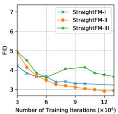
Figure 7: Comparison of the performance of FID using different StraightFM configuration during training.

Table 5: Configuration on CIFAR-10, CelebA-HQ and FFHQ.

	CIFAR-10		CelebA-HQ 256$\times$ 256		FFHQ 256$\times$ 256
	StraighFM-I	StraighFM-II	StraighFM-I	StraighFM-II	Inpainting Task
Architecture	NCSN++	NCSN++	ADM	ADM	NCSN++
Learning rate	2e-4	2e-4	2e-5	2e-5	2e-5
Batch size	4$\times$64	5$\times$64	4$\times$30	3$\times$40	2$\times$16
$\lambda$	0	10	0	10	0
Training iterations	600K	700K	1000K	850K	20K
EMA decay rate	0.999999	0.999999	0.9999	0.9999	0.999
GPUs	4$\times$ RTX 3090	5$\times$ RTX 4090	4$\times$Tesla V100	3$\times$Tesla V100	2$\times$TITAN RTX
Dropout probability	0.15	0.15	0.0	0.0	0.0

1.2 Implementation Details in the Latent Space

Our implementation in the latent space of Latent Diffusion Model on CelebA-HQ $256\times 256$ builds upon the open-source of LFM (Latent Flow Matching) [9]. Here, the structure of the velocity model utilizes a convolution-based UNet (ADM) [10]. The parameters are updated using exponential moving average (EMA) with a decay rate of 0.999. Other training configuration is comprehensively outlined in Tab. 5. For evaluation, we use torch-fidelity to assess both FID and KID metrics [35].

1.3 Implementation Details and Additional Results on Inpainting Task

We conduct the inpainting task on FFHQ $256\times 256$ dataset. In this procedure, we randomly mask 50% of the pixel values in the original images to create degraded images. After that, these degraded images serve as source samples from $p_{0}$, while corresponding original images can be regarded as target samples from $p_{1}$. Considering that these corresponding image pairs are natural optimal transport couplings, it is feasible to directly train a flow matching model using these image pairs.

For dataset splitting, FFHQ dataset, which consists of 70,000 high-resolution, well-aligned face images, is partitioned into two segments: the first 60,000 images for training and the remaining 10,000 for validation. The image quality assessment in this inpainting task is conducted with PyTorch Image Quality [18].

Under the same degradation configuration, our competitors include SNIPS and mGANPrior. SNIPS [19] is not originally designed for FFHQ dataset. The initial work in SNIPS directly calculates Singular Value Decomposition (SVD), which hinders its ability to process images with a resolution of 256$\times$ 256. To facilitate comparison, we replace this direct calculation with an efficient implementation, leveraging notable properties of SVD to reduce the space complexity to $O(n)$ [20].

Table 6: Hyper-parameters of mGNPrior on inpainting task.

Configuration	mGANPrior
Inversion type	StyleGAN-w+
Composing layer	4
Latent code number	30
Iterations	3000
Loss type	L2+VGG
Optimization	Adam

Another competitor, mGANPrior [12], employs a technique of optimizing multiple latent codes at certain intermediate layers of a pre-trained generator to generate feature maps for recovering the input image. Our reimplementation of mGANPrior based on StyleGAN [16], which is trained on the entire FFHQ dataset. Further configuration details are available in Tab. 6.

1.4 Visual examples

To better illustrate, additional synthesized examples from CIFAR-10 dataset are showcased in Fig. 8, Fig. 10 and Fig. 11. For CelebA-HQ 256 dataset, please refer to Fig. 9 and Fig. 12, and for FFHQ 256 dataset, relevant examples can be found in Fig. 13.

2 Discussion

2.1 Diffusion model and optimal transport

Although current diffusion models have achieved state-of-the-art performance in image generation, the comprehensive characterization and theoretical understanding of their connection to optimal transport is still not well-defined. A conjecture infers that diffusion model does not necessarily provide an optimal transport plan [24], but it only considers the limit case. On the other hand, recent work has found that diffusion model implicitly minimizes the Wasserstein distance [23]. Moreover, under certain conditions, the couplings derived from the PF-ODE of diffusion model coincide with an optimal transport map [21, 51]. Our extensive numerical experiments also reveal the high similarity of diffusion and flow matching models, where the latter yields a non-increasing transport cost. We believe that our analytical result will inspire other researchers to obtain a more generalized theoretical exploration.

2.2 Interrelationships among ODE-based generative models

Furthermore, the interrelationships among ODE-based generative models are not yet fully understood. There is a prevalent view that the coupling strategy of flow matching (i.e., the straightening procedure of Rectified Flow) is to find couplings superior to couplings from diffusion models [29]. Paradoxically, the mapping in Rectified Flow is largely consistent with diffusion models. This observation raises a significant question: Do all ODE-based generative models share this similarity and return to one optimal transport map? In the future, we will focus on the above question to explore a more efficient generative that fully leverages the capabilities of existing well-trained generative models.

2.3 Limitations of StraightFM

StraightFM yields straighter trajectories and high-quality images with few-step and one-step generation. However, the training of StraightFM mainly depends on the coupling mechanism derived from diffusion model sampling. Current diffusion models, while capable of generating samples within a reasonable range of 10-50 steps, exhibit a notable gap in sampling speed compared to random coupling strategy. Although current diffusion models can generate samples with acceptable 10-50 steps, there is still a gap in sampling speed compared to random coupling. To mitigate this issue, future studies could focus on examining the balance between the speed of coupling and the quality of samples in flow matching.

N=1

N=3

N=5

Adap.N

N=1

N=3

N=5

Adap.N

N=1

N=3

N=5

Adap.N

N=1

N=3

N=5

Adap.N

EDM

1-RF

2-RF

3-RF

Ours-I

Ours-II

EDM

1-RF

2-RF

3-RF

Ours-I

Ours-II

Figure 8: Comparison includes diffusion model (EDM), flow matching models (RF) and StraightFM (Ours) trained on CIFAR- 10 when simulated with fixed and adaptive steps (N). All corresponding samples are generated from the same initial noise.

LDM

LFM

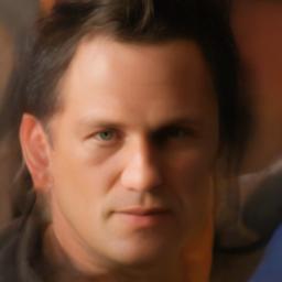
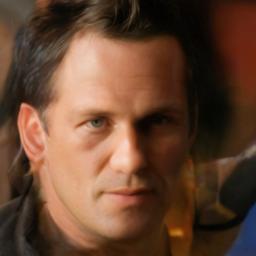
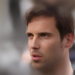
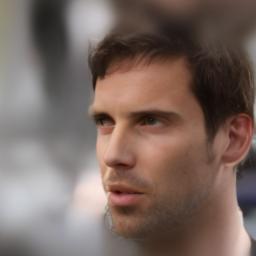
StraightFM-I

StraightFM-II

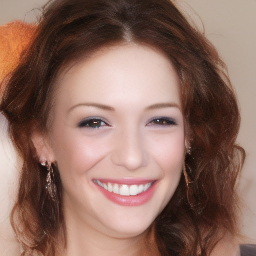
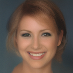
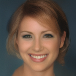
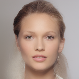
N=10

N=20

N=10

N=20

N=10

N=20

Figure 9: Comparison of samples generated on CelebA-HQ 256$\times$256 dataset with different sampling steps.

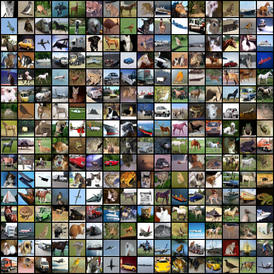
Figure 10: Uncurated samples from StraightFM-I on CIFAR-10.

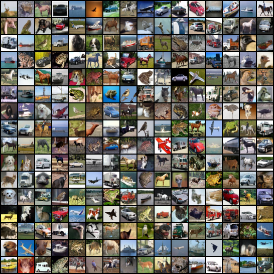
Figure 11: Uncurated samples from StraightFM-II on CIFAR-10.

(a) StraightFM-I

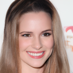
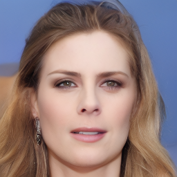
(b) StraightFM-II

Figure 12: Uncurated samples on CelebA-HQ $256\times 256$ from StraightFM-I (a) and StraightFM-II (b).

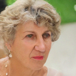
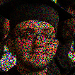
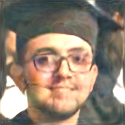
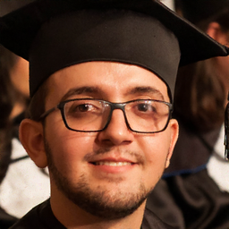
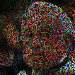
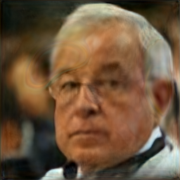
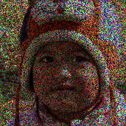
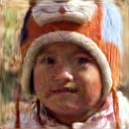
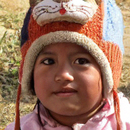
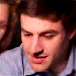
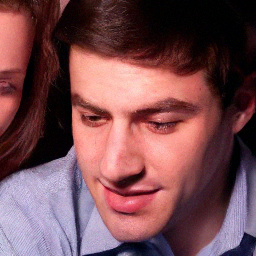
degraded

mGANPrior

SNIPS

Ours

Figure 13: Uncurated samples from FFHQ on inpainting task.

References

- Albergo and Vanden-Eijnden [2023] Michael Samuel Albergo and Eric Vanden-Eijnden. Building normalizing flows with stochastic interpolants. In ICLR, 2023.
- Alemohammad et al. [2023] Sina Alemohammad, Josue Casco-Rodriguez, Lorenzo Luzi, Ahmed Imtiaz Humayun, Hossein Babaei, Daniel LeJeune, Ali Siahkoohi, and Richard G Baraniuk. Self-consuming generative models go mad. In ICLR, 2023.
- Bao et al. [2021] Fan Bao, Chongxuan Li, Jun Zhu, and Bo Zhang. Analytic-dpm: an analytic estimate of the optimal reverse variance in diffusion probabilistic models. In ICLR, 2021.
- Ben Fei and Zhang [2023] Liang Pan Ben Fei, Zhaoyang Lyu and Junzhe Zhang. Generative diffusion prior for unified image restoration and enhancement. In CVPR, 2023.
- Bińkowski et al. [2018] Mikołaj Bińkowski, Danica J Sutherland, Michael Arbel, and Arthur Gretton. Demystifying mmd gans. In ICLR, 2018.
- Chen et al. [2020] Nanxin Chen, Yu Zhang, Heiga Zen, Ron J Weiss, Mohammad Norouzi, and William Chan. Wavegrad: Estimating gradients for waveform generation. In ICLR, 2020.
- Chen et al. [2018] Ricky TQ Chen, Yulia Rubanova, Jesse Bettencourt, and David K Duvenaud. Neural ordinary differential equations. NeurIPS, 31, 2018.
- Chen et al. [2021] Tianrong Chen, Guan-Horng Liu, and Evangelos Theodorou. Likelihood training of schrödinger bridge using forward-backward sdes theory. In ICLR, 2021.
- Dao et al. [2023] Quan Dao, Hao Phung, Binh Nguyen, and Anh Tran. Flow matching in latent space. arXiv preprint arXiv:2307.08698, 2023.
- Dhariwal and Nichol [2021] Prafulla Dhariwal and Alexander Nichol. Diffusion models beat gans on image synthesis. NeurIPS, 34:8780–8794, 2021.
- Grathwohl et al. [2018] Will Grathwohl, Ricky TQ Chen, Jesse Bettencourt, Ilya Sutskever, and David Duvenaud. Ffjord: Free-form continuous dynamics for scalable reversible generative models. In ICLR, 2018.
- Gu et al. [2020] Jinjin Gu, Yujun Shen, and Bolei Zhou. Image processing using multi-code gan prior. In CVPR, pages 3012–3021, 2020.
- Heusel et al. [2017] Martin Heusel, Hubert Ramsauer, Thomas Unterthiner, Bernhard Nessler, and Sepp Hochreiter. Gans trained by a two time-scale update rule converge to a local nash equilibrium. NeurIPS, 30, 2017.
- Ho et al. [2020] Jonathan Ho, Ajay Jain, and Pieter Abbeel. Denoising diffusion probabilistic models. NeurIPS, 33:6840–6851, 2020.
- Karras et al. [2018] Tero Karras, Timo Aila, Samuli Laine, and Jaakko Lehtinen. Progressive growing of gans for improved quality, stability, and variation. In ICLR, 2018.
- Karras et al. [2019] Tero Karras, Samuli Laine, and Timo Aila. A style-based generator architecture for generative adversarial networks. In CVPR, pages 4401–4410, 2019.
- Karras et al. [2022] Tero Karras, Miika Aittala, Timo Aila, and Samuli Laine. Elucidating the design space of diffusion-based generative models. NeurIPS, 2022.
- Kastryulin et al. [2022] Sergey Kastryulin, Jamil Zakirov, Denis Prokopenko, and Dmitry V. Dylov. Pytorch image quality: Metrics for image quality assessment, 2022.
- Kawar et al. [2021] Bahjat Kawar, Gregory Vaksman, and Michael Elad. Snips: Solving noisy inverse problems stochastically. NeurIPS, 34:21757–21769, 2021.
- Kawar et al. [2022] Bahjat Kawar, Michael Elad, Stefano Ermon, and Jiaming Song. Denoising diffusion restoration models. NeurIPS, 35:23593–23606, 2022.
- Khrulkov et al. [2022] Valentin Khrulkov, Gleb Ryzhakov, Andrei Chertkov, and Ivan Oseledets. Understanding ddpm latent codes through optimal transport. In ICLR, 2022.
- Krizhevsky et al. [2009] Alex Krizhevsky et al. Learning multiple layers of features from tiny images. 2009.
- Kwon et al. [2022] Dohyun Kwon, Ying Fan, and Kangwook Lee. Score-based generative modeling secretly minimizes the wasserstein distance. NeurIPS, 35:20205–20217, 2022.
- Lavenant and Santambrogio [2022] Hugo Lavenant and Filippo Santambrogio. The flow map of the fokker–planck equation does not provide optimal transport. Applied Mathematics Letters, 133:108225, 2022.
- Le et al. [2023] Matthew Le, Apoorv Vyas, Bowen Shi, Brian Karrer, Leda Sari, Rashel Moritz, Mary Williamson, Vimal Manohar, Yossi Adi, Jay Mahadeokar, et al. Voicebox: Text-guided multilingual universal speech generation at scale. NeurIPS, 2023.
- Lee et al. [2023] Sangyun Lee, Beomsu Kim, and Jong Chul Ye. Minimizing trajectory curvature of ode-based generative models. In ICML, 2023.
- Lipman et al. [2022] Yaron Lipman, Ricky TQ Chen, Heli Ben-Hamu, Maximilian Nickel, and Matthew Le. Flow matching for generative modeling. In ICLR, 2022.
- Liu et al. [2021] Luping Liu, Yi Ren, Zhijie Lin, and Zhou Zhao. Pseudo numerical methods for diffusion models on manifolds. In ICLR, 2021.
- Liu et al. [2022] Xingchao Liu, Chengyue Gong, et al. Flow straight and fast: Learning to generate and transfer data with rectified flow. In ICLR, 2022.
- Liu et al. [2023] Xingchao Liu, Xiwen Zhang, Jianzhu Ma, Jian Peng, and Qiang Liu. Instaflow: One step is enough for high-quality diffusion-based text-to-image generation. arXiv preprint arXiv:2309.06380, 2023.
- Lu et al. [2022] Cheng Lu, Yuhao Zhou, Fan Bao, Jianfei Chen, Chongxuan Li, and Jun Zhu. Dpm-solver: A fast ode solver for diffusion probabilistic model sampling in around 10 steps. NeurIPS, 35:5775–5787, 2022.
- Luo and Hu [2021] Shitong Luo and Wei Hu. Diffusion probabilistic models for 3d point cloud generation. In CVPR, 2021.
- Meng et al. [2023] Chenlin Meng, Robin Rombach, Ruiqi Gao, Diederik Kingma, Stefano Ermon, Jonathan Ho, and Tim Salimans. On distillation of guided diffusion models. In CVPR, pages 14297–14306, 2023.
- Nichol and Dhariwal [2021] Alexander Quinn Nichol and Prafulla Dhariwal. Improved denoising diffusion probabilistic models. In ICML, pages 8162–8171. PMLR, 2021.
- Obukhov et al. [2020] Anton Obukhov, Maximilian Seitzer, Po-Wei Wu, Semen Zhydenko, Jonathan Kyl, and Elvis Yu-Jing Lin. High-fidelity performance metrics for generative models in pytorch, 2020. Version: 0.3.0, DOI: 10.5281/zenodo.4957738.
- Pooladian et al. [2023] Aram-Alexandre Pooladian, Heli Ben-Hamu, Carles Domingo-Enrich, Brandon Amos, Yaron Lipman, and Ricky Chen. Multisample flow matching: Straightening flows with minibatch couplings. In ICML, 2023.
- Rombach et al. [2022] Robin Rombach, Andreas Blattmann, Dominik Lorenz, Patrick Esser, and Björn Ommer. High-resolution image synthesis with latent diffusion models. In CVPR, pages 10684–10695, 2022.
- Salimans and Ho [2021] Tim Salimans and Jonathan Ho. Progressive distillation for fast sampling of diffusion models. In ICLR, 2021.
- Salimans et al. [2016] Tim Salimans, Ian Goodfellow, Wojciech Zaremba, Vicki Cheung, Alec Radford, and Xi Chen. Improved techniques for training gans. NeurIPS, 29, 2016.
- Sohl-Dickstein et al. [2015] Jascha Sohl-Dickstein, Eric Weiss, Niru Maheswaranathan, and Surya Ganguli. Deep unsupervised learning using nonequilibrium thermodynamics. In ICML, pages 2256–2265. PMLR, 2015.
- Song et al. [2020a] Jiaming Song, Chenlin Meng, and Stefano Ermon. Denoising diffusion implicit models. In ICLR, 2020a.
- Song et al. [2020b] Yang Song, Jascha Sohl-Dickstein, Diederik P Kingma, Abhishek Kumar, Stefano Ermon, and Ben Poole. Score-based generative modeling through stochastic differential equations. In ICLR, 2020b.
- Song et al. [2023] Yang Song, Prafulla Dhariwal, Mark Chen, and Ilya Sutskever. Consistency models. In ICML, 2023.
- Tanaka [2019] Akinori Tanaka. Discriminator optimal transport. NeurIPS, 32, 2019.
- Tong et al. [2023a] Alexander Tong, Nikolay Malkin, Guillaume Huguet, Yanlei Zhang, Jarrid Rector-Brooks, Kilian Fatras, Guy Wolf, and Yoshua Bengio. Conditional flow matching: Simulation-free dynamic optimal transport. arXiv preprint arXiv:2302.00482, 2023a.
- Tong et al. [2023b] Alexander Tong, Nikolay Malkin, Guillaume Huguet, Yanlei Zhang, Jarrid Rector-Brooks, Kilian Fatras, Guy Wolf, and Yoshua Bengio. Improving and generalizing flow-based generative models with minibatch optimal transport. In Int. Conf. Machi. Learning. Worksh., 2023b.
- Wang et al. [2021] Gefei Wang, Yuling Jiao, Qian Xu, Yang Wang, and Can Yang. Deep generative learning via schrödinger bridge. In ICML, pages 10794–10804. PMLR, 2021.
- Wang et al. [2004] Zhou Wang, Alan C Bovik, Hamid R Sheikh, and Eero P Simoncelli. Image quality assessment: from error visibility to structural similarity. IEEE TIP, 13(4):600–612, 2004.
- Wu et al. [2023] Lemeng Wu, Dilin Wang, Chengyue Gong, Xingchao Liu, Yunyang Xiong, Rakesh Ranjan, Raghuraman Krishnamoorthi, Vikas Chandra, and Qiang Liu. Fast point cloud generation with straight flows. In CVPR, pages 9445–9454, 2023.
- Xiao et al. [2021] Zhisheng Xiao, Karsten Kreis, and Arash Vahdat. Tackling the generative learning trilemma with denoising diffusion gans. In ICLR, 2021.
- Zhang et al. [2023] Pengze Zhang, Hubery Yin, Chen Li, and Xiaohua Xie. Formulating discrete probability flow through optimal transport. NeurIPS, 2023.
- Zhang and Chen [2022] Qinsheng Zhang and Yongxin Chen. Fast sampling of diffusion models with exponential integrator. In ICLR, 2022.
- Zhang et al. [2018] Richard Zhang, Phillip Isola, Alexei A Efros, Eli Shechtman, and Oliver Wang. The unreasonable effectiveness of deep features as a perceptual metric. In CVPR, pages 586–595, 2018.
- Zhao et al. [2023] Wenliang Zhao, Lujia Bai, Yongming Rao, Jie Zhou, and Jiwen Lu. Unipc: A unified predictor-corrector framework for fast sampling of diffusion models. NeurIPS, 2023.