Revealing novel aspects of light-matter coupling in terahertz two-dimensional coherent spectroscopy: the case of the amplitude mode in superconductors

Abstract

Recently developed terahertz (THz) two-dimensional coherent spectroscopy (2DCS) is a powerful technique to obtain materials information in a fashion qualitatively different from other spectroscopies. Here, we utilized THz 2DCS to investigate the THz nonlinear response of conventional superconductor NbN. Using broad-band THz pulses as light sources, we observed a third-order nonlinear signal whose spectral components are peaked at twice the superconducting gap energy $2\Delta$. With narrow-band THz pulses, a THz nonlinear signal was identified at the driving frequency $\Omega$ and exhibited a resonant enhancement at temperature when $\Omega=2\Delta$. General theoretical considerations show that such a resonance can only arise from a disorder-activated paramagnetic coupling between the light and the electronic current. This proves that the nonlinear THz response can access processes distinct from the diamagnetic Raman-like density fluctuations, which are believed to dominate the nonlinear response at optical frequencies in metals. Our numerical simulations reveal that even for a small amount of disorder, the $\Omega=2\Delta$ resonance is dominated by the superconducting amplitude mode over the entire investigated disorder range. This is in contrast to other resonances, whose amplitude-mode contribution depends on disorder. Our findings demonstrate the unique ability of THz 2DCS to explore collective excitations inaccessible in other spectroscopies.

A transition to a state of matter that spontaneously breaks a continuous $U(1)$ symmetry of the Hamiltonian is characterized by the emergence of collective electronic modes associated with amplitude and phase fluctuations of the complex order parameter [1, 2]. The finite energy amplitude mode is an analog of the Higgs boson associated with the electroweak symmetry breaking of the fundamental vacuum [1, 2]. In condensed matter physics, amplitude modes have been explored in various ordered phases, such as charge density waves (CDW) [3, 4, 5, 6], antiferromagnets [7, 8, 9], and superfluid ³He [10, 11]. In the case of superconductors, long-range Coulomb interaction pushes the otherwise massless phase mode up to the plasma frequency, while the amplitude mode stays intact at twice the SC gap energy $2\Delta$ [1, 2]. The observation of the amplitude mode in superconductors is challenging because it does not couple linearly to light being charge neutral, and it is expected to have a weak Raman response  [12, 13, 14] in cases when spontaneous Raman scattering can be interpreted as a probe of density fluctuations [15]. An exception is the case of 2$H$-NbSe₂ [16, 17, 18, 19, 20] or 2$H$-TaS₂ [21] where superconductivity coexists with CDW order and the amplitude mode can be seen in Raman spectroscopy by virtue of its coupling to the Raman-active soft CDW phonon [22, 20].

With the aim of identifying the amplitude mode in superconductors, the THz nonlinear optical response has been explored. THz nonlinear responses, such as pump-probe response or third-harmonic generation (THG) in a conventional superconductor NbN, have been initially interpreted as the excitation of an amplitude mode through a nonlinear coupling to the electromagnetic field  [23, 24, 25, 26, 2]. Since then, the THz nonlinear response has been extensively explored in superconductors like MgB₂ [27, 28, 29], high-temperature cuprates [30, 31, 32, 33, 34], and iron-based systems [35, 36, 37, 38, 39]. Motivated by these experiments, theoretical works have shown that the third-harmonic (TH) THz nonlinear response is governed by quasiparticle excitations as well as the amplitude mode, with a relative hierarchy of the two contributions that depends on the disorder level and pairing strength  [12, 40, 41, 42, 43, 44, 45, 13, 46, 47]. Importantly, theoretical considerations highlighted the possibility that THz nonlinearities can be mediated by an intrinsically different electronic response as compared to conventional nonlinearities at optical frequencies of a few eV  [42, 13, 44]. In principle, the latter is governed by diamagnetic Raman-like density-density scattering in metals  [15], whereas even weak disorder may allow THz light to trigger paramagnetic current-current fluctuations. Nevertheless, clear experimental indication of the predominance of paramagnetic processes has not been reported.

Toward this aim, the recently developed multi-dimensional coherent spectroscopy is promising as it may allow one to disentangle different nonlinear processes [48]. In the case of THz two-dimensional coherent spectroscopy (2DCS), magnon [49], phonon [50], plasmon [51], and electronic excitations in disordered systems [52] have been clearly identified. In this Letter, we investigated the THz nonlinear response of the dirty-limit conventional superconductor NbN by THz 2DCS. Using broad-band THz, we observed a nonlinear signal peaked at twice the SC gap energy $2\Delta$. As the temperature increases, this nonlinear signal’s peak exhibits a redshift following the temperature dependence of $2\Delta$ obtained from the equilibrium optical response. To resolve the origin of these nonlinear spectral features, we employed narrow-band THz pulses at the driving angular frequency $\Omega/2\pi$ = 0.63 THz for THz 2DCS. We identified a first-harmonic (FH) nonlinear signal whose intensity displays a resonant enhancement when $2\Delta$ matches the driving frequency $\Omega$. General theoretical considerations show that this FH signal, inaccessible in previous works focusing on THG, can only be generated by the aforementioned paramagnetic processes. Our numerical simulations demonstrate that with finite disorder, the $\Omega=2\Delta$ resonance of the FH response is dominated by the amplitude mode, offering a preferential route for its detection.

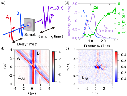
Figure 1: (a) A schematic of the THz 2DCS experiment. (b) Time traces of the A and B pulses together ($E_{AB}(t,\tau)$) transmitted after the NbN sample ($T_{\text{c}}$ = 14.9 K) at 5 K as a function of the sampling time $t$ and the delay time $\tau$. (c) The same plot as (b) but for the nonlinear signal $E_{NL}(t,\tau)$. (d) Power spectrum of the THz nonlinear signal from NbN at 5 K measured at $\tau=0$ ps with the broad-band THz pulses (purple, left axis). The blue dashed curve on the left axis is the power spectrum of the B-pulse. The green curve on the right axis shows the real part of the optical conductivity at 5 K.

The schematic of the experiment is depicted in Fig. 1(a). Two intense single-cycle (broad-band) THz pulses are generated using the tilted-pulse front technique with LiNbO₃ [53, 54, 55]. See the Supplemental Material (SM) [56] for details. We first performed THz 2DCS on NbN ($T_{\text{c}}$ = 14.9 K) using broad-band THz pulses. The peak $E$-field of A and B pulses did not exceed 3 kV/cm to avoid the depletion of the SC condensate. We measured the transmitted THz $E$-fields of two pulses ($E_{A}(t,\tau)$, $E_{B}(t)$) separately, and of both pulses ($E_{AB}(t,\tau)$) together as shown in Fig. 1(b). We swept the delay time $\tau$ of the A-pulse with respect to the arrival of the B-pulse. The nonlinear signal’s $E$-field is obtained as $E_{NL}(t,\tau)=E_{AB}(t,\tau)-E_{A}(t,\tau)-E_{B}(t)$, presented in Fig. 1(c). We perform a Fourier transform with respect to $t$, or both $t$ and $\tau$. Fig. 1(d) shows the power spectrum of the nonlinear signal at 5 K when $\tau=0$ ps (the purple curve). The nonlinear signal exhibits two peaks: one matches twice the SC gap $2\Delta$ identified in the THz optical conductivity measured at 5 K (the green curve on the right axis), and the other is located at slightly higher energy than the center frequency of the B-pulse.

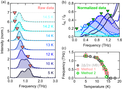
Figure 2: (a) Power spectrum of the nonlinear signal from NbN ($T_{\text{c}}$ = 14.9 K) when $\tau=0$ ps at different temperatures with single-cycle THz pulses. The gray dashed curves denote the fit to the data using a Lorentzian multiplied by the B-pulse power spectra. The obtained peak energy is presented by the red triangles. (b) The nonlinear signal in (a) divided by the B-pulse power spectra as a function of temperature. The obtained peak energy with fitting is shown by the green triangles. The dashed curves are the fits to the data using a Lorentzian. (c) Peak energy of the nonlinear signal as a function of temperature obtained by fitting the raw data in (a) (red open squares) and the normalized data in (b) (green open diamonds). The gray circles are the temperature dependence of the gap evaluated using the Mattis-Bardeen model.

In Fig. 2(a), we present the power spectrum of the nonlinear signal at $\tau=0$ ps measured at different temperatures. The peak energy in the nonlinear signal shows a redshift with increasing temperature. We evaluated the energy of the peak in two ways. First, we fit the power spectra of the nonlinear signal using the power spectrum of the B-pulse multiplied by a Lorentzian. The fits reasonably reproduce the data as presented by the gray dashed curves in Fig. 2(a). The extracted peak energy is plotted as a function of temperature by red open squares in Fig. 2(c), in good agreement with the temperature dependence of $2\Delta$ (the gray circles) as seen in the linear responses. We also evaluated the peak energy by normalizing the nonlinear signal spectra with the B-pulse spectra, as shown in Fig. 2(b). While the normalized spectra display an increasing tendency toward higher frequency below 12 K, likely due to the THG signal, peaks are discerned in the frequency range from 0.3 to 1.4 THz. We fit the normalized spectrum with a Lorentzian and plot the obtained peak energy as a function of temperature by green open diamonds in Fig. 2(c), consistent with those in the first procedure. This direct correspondence between the peak energy of the nonlinear signal and the SC gap energy was also found in other NbN samples with different $T_{\text{c}}$, as presented in Fig. S2 in the SM.

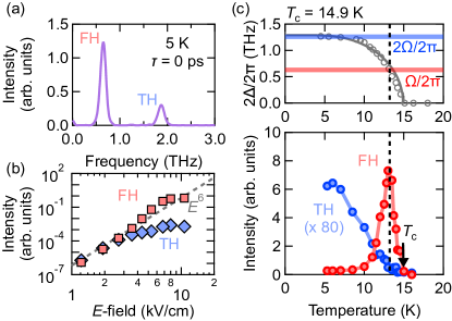
Figure 3: (a) Power spectrum of the THz nonlinear signal at 5 K measured at $\tau=0$ ps with narrow-band THz pulses. (b) The frequency-integrated intensity of the FH and TH contributions at 5 K when $\tau=0$ ps as a function of the B-pulse peak $E$-field. The dashed gray curve is the guide to the eye with a slope of 6. (c) Temperature dependence of the frequency-integrated intensity of the FH (red) and TH (blue) contributions. The top presents the temperature dependence of $2\Delta$ evaluated from the linear conductivity as compared to $\Omega$ (red) and $2\Omega$ (blue). The solid gray curve is the gap computed by numerically solving the BCS equation. The black dashed line denotes the temperature that satisfies $\Omega=2\Delta$.

To obtain deeper insight into the spectrum of the nonlinear signal, we performed THz 2DCS using narrow-band THz pulses with the peak $E$-field of 3 kV/cm and a driving angular frequency of $\Omega/2\pi$ = 0.63 THz. Figure 3(a) shows the nonlinear signal spectra for NbN with $T_{\text{c}}$ = 14.9 K measured at 5 K when $\tau=0$ ps. The power spectrum exhibits two peaks at 0.63 THz and 1.9 THz, corresponding to the FH and TH contributions, respectively. Both FH and TH intensities follow $E^{6}$ as shown in Fig. 3(b) up to the THz peak $E$-field $E$ of 10 and 4 kV/cm, respectively, indicating that both are third-order nonlinear responses. In the third-order processes driven at a frequency $\Omega$, the nonlinear signals are generated at frequencies of $\pm\Omega\pm\Omega\pm\Omega$ [57], giving signals at $\Omega$ and 3$\Omega$.

Figure 3(c) shows the frequency-integrated intensity of the FH and TH signals as a function of temperature with the multi-cycle THz pulses when $\tau=0$ ps. Here, we integrate from 0.3 to 1 THz for the FH signal, and from 1.6 to 2.2 THz for the TH signal. The temperature dependence of the TH signal is consistent with the previous reports where it takes its maximum intensity when twice the drive frequency matches twice the SC gap energy $2\Delta$ (i.e. $2\Omega=2\Delta$) as shown in the top panel [23, 24, 26, 2]. By contrast, the FH signal displays a resonant enhancement when the driving frequency matches $2\Delta$ (i.e. $\Omega=2\Delta$). These behaviors were found in the other NbN samples with different $T_{\text{c}}$, as shown in Fig. S3 in SM. This FH signal has been overlooked in previous THz nonlinear experiments because it is usually overwhelmed by the transmitted $E$-field at the FH primarily from linear transmission. The difference-signal analysis inherent to 2DCS allows it to be isolated here. It is worth mentioning that this FH signal is not resolvable in the strong-pump weak-probe THz 2DCS-like experiments reported previously [25], as it derives from a single pump photon and two probe photons (see SM).

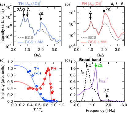
Figure 4: (a),(b) Nonlinear current intensity $|J_{NL}|^{2}$ for the (a) TH and (b) FH components as a function of the driving frequency $\Omega$ normalized by the SC gap $\Delta$ for the BCS contribution (dashed curve) and the sum of the BCS and amplitude-mode contributions (solid curves). (c) Comparison between the experimental data (open circles) and the theoretical results (solid curves) for the temperature dependence of the FH (red) and TH (blue). The temperature $T$ is normalized by $T_{\text{c}}$. To remove the temperature-dependent screening effects, the experimental nonlinear signal intensity ($|E_{NL}|^{2}$) is normalized by the internal B-pulse $E$-field ($E_{B}^{6}$) (see [56]). The theoretical results correspond to the nonlinear current intensity $|J_{NL}|^{2}$ at the driving frequency of 0.63 THz for a $E$-field constant in temperature. (d) The nonlinear current simulated using the broadband THz pulses. The black dashed curve shows the intensity of the driving THz $E$-field, obtained by simulating the experimental THz B-pulse.

To clarify the experimental observations, we analyze the different nonlinear processes following the diagrammatic approach in previous work [12, 42, 43, 44]. The nonlinear processes in the SC state can be obtained by combining the diamagnetic (quadratic) and paramagnetic (linear) couplings between electronic excitation and the electromagnetic field. In the diagrammatic representation, the former is represented as a density-like electronic vertex with two-photon lines attached, while the latter appears as current-like electronic vertex with a single-photon line. The third-order nonlinear current is generally expressed as $J_{NL}(\omega)=\int\text{d}\omega_{1}\text{d}\omega_{2}\text{d}\omega_{3}\delta(\omega_{1}+\omega_{2}+\omega_{3}-\omega)A(\omega_{1})A(\omega_{2})A(\omega_{3})K(\omega_{1},\omega_{2},\omega_{3})$, where $A(\omega)$ denotes the gauge field. Assuming monochromatic fields ($\omega_{i}=\pm\Omega$ for $i=1,2,3$), the possible combinations of $\omega_{i}$ gives peaks at $\omega=\Omega$ and $\omega=3\Omega$ in $J_{NL}(\omega)$. The spectral structure simplifies in the clean limit, when only diamagnetic processes are allowed [12]. Because diamagnetic vertices have two-photon lines attached, the nonlinear kernel $K$ can be reduced to $K^{dia}(\omega_{1}+\omega_{2})$ and its frequency permutations. Given that the quasiparticles and amplitude-mode fluctuations are both enhanced at $2\Delta$, both the FH and TH diamagnetic responses are largest when $\omega_{1}+\omega_{2}=2\Delta$ and thus for single-frequency driving at $\Omega$, their resonance occurs at $\Omega=\Delta$ [12, 56].

In contrast, when a finite amount of disorder is included, paramagnetic processes become allowed. Consequently, as detailed in the SM, the nonlinear kernel is a function $K^{para}(\omega_{1},\omega_{1}+\omega_{2},\omega_{1}+\omega_{2}+\omega_{3})$, plus permutations of the running-frequencies, and one expects an enhancement whenever any of the three arguments of $K^{para}$ matches $2\Delta$. Therefore, unlike the resonance at $\Omega=\Delta$ for the FH and TH responses, the FH response at $\Omega=2\Delta$, and TH responses at $\Omega=2\Delta/3$ and $\Omega=2\Delta$ can only arise via paramagnetic processes. They are absent in the usual description of optical nonlinearity based on the diamagnetic Raman-like response within the widely-used effective-mass approximation for conductors [15].

We examined these expectations by numerical simulations using the attractive Hubbard model on a square lattice with Anderson-type impurities. Following the approach in Ref. [44, 46], we computed the nonlinear TH and FH signals, as shown in Figs. 4(a) and (b), respectively. Here, we set the disorder level to $k_{F}l=6$ ($k_{F}$ is the Fermi wave vector and $l$ is the electronic mean free path) and evaluated the BCS-quasiparticle contribution (the dashed curves, denoted as BCS) and the sum of it and the amplitude-mode contribution (the solid curves, denoted as BCS + AM) separately (see SM for details). For the TH signal, the nonlinear current is enhanced at the expected three possible frequency combinations, as denoted by the vertical arrows in Fig. 4(a). In the SM, we show that the relative ratio between the BCS and amplitude-mode contributions for the lower two peaks is consistent with previous reports [42, 43, 44], where the amplitude mode acquires considerable spectral weight for very strong disorder. On the other hand, we find that the upper peak at $\Omega=2\Delta$, not investigated so far, is dominated by the amplitude mode for both $k_{F}l=6$ and also the more disordered case of $k_{F}l=4$ shown in Fig. S7. The FH $J_{NL}(\Omega)$ has two features that correspond to the two allowed frequencies for the FH response as discussed above. Again, the amplitude mode dominates the upper resonance for all disorder levels investigated, whereas the lower energy resonance shows appreciable disorder dependence. We note that the dominance of the amplitude mode at $\Omega=2\Delta$ in both TH and FH responses is an empirical observation from our numerics. The reason for it is a topic of current investigation.

Next, we compute the temperature dependence of the FH and TH signals at $\Omega/2\pi$ = 0.63 THz by modeling the kernel resonances numerically, using the temperature dependence of the SC gap obtained from the linear responses (see SM). Figure 4(c) compares the numerical results with the experimental data normalized by the incoming THz $E$-field for the FH and TH components. The calculated result for the FH component displays excellent agreement with experiments, unambiguously indicating that the FH signal stems from the amplitude-mode contribution at $\Omega=2\Delta$ via the paramagnetic processes. The numerical result for the TH component displays a monotonic increase when the temperature is lowered, consistent with the experimental data. The increase in the TH intensity toward the lower temperature is due to the resonance of $\Omega=\Delta$ around 0 K, which is likely dominated by the amplitude mode in the high disorder level relevant for NbN. To check the internal consistency of our approach, we further simulate the nonlinear current driven by broad-band THz pulses (see SM for details). Figure 4(d) presents the nonlinear current induced by the broad-band THz pulses for $2\Delta/2\pi$ = 1.2 THz. The computed nonlinear current exhibits three peaks at $\Omega/2\pi=0.63$ THz, $2\Delta/2\pi$ = 1.2 THz, and $3\Omega/2\pi=1.9$ THz, qualitatively reproducing the experimental observation in Fig. 1(d).

Finally, to understand the full time evolution of the THz 2DCS response induced by single-cycle THz pulses for different delay times $\tau$, we modeled the time evolution of the nonlinear signal in close analogy with the previously discussed results (see SM). In particular, we modeled the largest contribution of the coherent response by a nonlinear kernel peaked at $2\Delta$, and additionally included a phenomenological incoherent kernel describing the out-of-equilibrium quasiparticle relaxation. Figure S12(b) presents the simulated 2D spectra that qualitatively reproduces the data in Fig. S12(a).

In summary, we reported the THz nonlinear signal in conventional superconductors NbN using THz 2DCS. Using broad-band THz pulses, we identified a prominent spectral component of the nonlinear signal peaked at twice the SC gap energy $2\Delta$. With narrow-band THz pulses, the same nonlinear signal appeared at the driving THz frequency $\Omega$, in a fashion inaccessible in previous experiments. By varying the temperature, it manifests a resonant enhancement when $\Omega=2\Delta$. General theoretical analysis showed that this resonance at $\Omega=2\Delta$ in the nonlinear kernel can only arise from a paramagnetic coupling of photons to electronic current. Our numerical simulations revealed that this resonance in the paramagnetic nonlinear current is dominated by the amplitude mode of the SC order parameter.

Our work not only establishes the ability of THz 2DCS to access light-matter interactions unresolvable by previous THG or pump-probe experiments, but it also unambiguously demonstrates the intrinsic difference between the excitation processes contributing to the THz nonlinear response as compared to the optical nonlinearity that is usually understood by analogy to spontaneous non-resonant Raman spectroscopy. These results open a novel perspective on the ability of THz 2DSC to detect and/or drive other collective excitations such as the Leggett mode in multi-band superconductors [27, 58], the Bardasis-Schrieffer mode in iron-based superconductors [59, 37], or the Josephson plasmon in cuprate superconductors [60, 61, 62, 63, 64, 65, 66].

We acknowledge Y. Gallais, S. Houver, A.-M. Tremblay, and R. Matsunaga for discussions. This project was supported by the Gordon and Betty Moore Foundation, EPiQS initiative, Grant No. GBMF-9454 and NSF-DMR 2226666, by the Sapienza University under Ateneo projects RM12117A4A7FD11B and RP1221816662A977. and by the European Union under grant ERC-SYN, MORE-TEM, GA 951215. K.K. was supported by Overseas Research Fellowship of the JSPS. N.P.A., L.B., and J.F. acknowledge the hospitality of the KITP (QUASIPART23 program), through support of NSF under Grant Nos. NSF PHY-1748958 and NSF PHY-2309135. P.R. and J.J. acknowledge the Department of Atomic Energy, Government of India (Grant 12-R & D-TFR-5.10- 0100). G.S. acknowledges financial support from the Deutsche Forschungsgemeinschaft under SE 80/20-1.

References

- Pekker and Varma [2015] D. Pekker and C. M. Varma, Annu. Rev. Condens. Matter Phys. 6, 269 (2015).
- Shimano and Tsuji [2020] R. Shimano and N. Tsuji, Annu. Rev. Condens. Matter Phys. 11, 103 (2020).
- Tsang et al. [1976] J. C. Tsang, J. E. Smith, and M. W. Shafer, Phys. Rev. Lett. 37, 1407 (1976).
- Demsar et al. [1999] J. Demsar, K. Biljaković, and D. Mihailovic, Phys. Rev. Lett. 83, 800 (1999).
- Sugai et al. [2006] S. Sugai, Y. Takayanagi, and N. Hayamizu, Phys. Rev. Lett. 96, 137003 (2006).
- Yusupov et al. [2010] R. Yusupov, T. Mertelj, V. V. Kabanov, S. Brazovskii, P. Kusar, J. H. Chu, I. R. Fisher, and D. Mihailovic, Nat. Phys. 6, 681 (2010).
- Rüegg et al. [2008] C. Rüegg, B. Normand, M. Matsumoto, A. Furrer, D. F. McMorrow, K. W. Krämer, H. U. Güdel, S. N. Gvasaliya, H. Mutka, and M. Boehm, Phys. Rev. Lett. 100, 205701 (2008).
- Merchant et al. [2014] P. Merchant, B. Normand, K. Krämer, M. Boehm, D. McMorrow, and C. Rüegg, Nat. Phys. 10, 373 (2014).
- Jain et al. [2017] A. Jain, M. Krautloher, J. Porras, G. Ryu, D. Chen, D. Abernathy, J. Park, A. Ivanov, J. Chaloupka, G. Khaliullin, et al., Nat. Phys. 13, 633 (2017).
- Lee [1998] D. M. Lee, J. Phys. Chem. Solids 59, 1682 (1998).
- Volovik and Zubkov [2014] G. Volovik and M. Zubkov, J. Low Temp. Phys. 175, 486 (2014).
- Cea et al. [2016] T. Cea, C. Castellani, and L. Benfatto, Phys. Rev. B 93, 180507(R) (2016).
- Udina et al. [2022] M. Udina, J. Fiore, T. Cea, C. Castellani, G. Seibold, and L. Benfatto, Faraday Discuss. 237, 168 (2022).
- Benfatto et al. [2022] L. Benfatto, C. Castellani, and T. Cea, Phys. Rev. Lett. 129, 199701 (2022).
- Devereaux and Hackl [2007] T. P. Devereaux and R. Hackl, Rev. Mod. Phys. 79, 175 (2007).
- Sooryakumar and Klein [1980] R. Sooryakumar and M. V. Klein, Phys. Rev. Lett. 45, 660 (1980).
- Littlewood and Varma [1981] P. B. Littlewood and C. M. Varma, Phys. Rev. Lett. 47, 811 (1981).
- Littlewood and Varma [1982] P. B. Littlewood and C. M. Varma, Phys. Rev. B 26, 4883 (1982).
- Méasson et al. [2014] M. A. Méasson, Y. Gallais, M. Cazayous, B. Clair, P. Rodière, L. Cario, and A. Sacuto, Phys. Rev. B 89, 060503 (2014).
- Grasset et al. [2018] R. Grasset, T. Cea, Y. Gallais, M. Cazayous, A. Sacuto, L. Cario, L. Benfatto, and M.-A. Méasson, Phys. Rev. B 97, 094502 (2018).
- Grasset et al. [2019] R. Grasset, Y. Gallais, A. Sacuto, M. Cazayous, S. Mañas Valero, E. Coronado, and M.-A. Méasson, Phys. Rev. Lett. 122, 127001 (2019).
- Cea and Benfatto [2016] T. Cea and L. Benfatto, Phys. Rev. B 94, 064512 (2016).
- Matsunaga et al. [2014] R. Matsunaga, N. Tsuji, H. Fujita, A. Sugioka, K. Makise, Y. Uzawa, H. Terai, Z. Wang, H. Aoki, and R. Shimano, Science 345, 1145 (2014).
- Tsuji and Aoki [2015] N. Tsuji and H. Aoki, Phys. Rev. B 92, 064508 (2015).
- Matsunaga and Shimano [2015] R. Matsunaga and R. Shimano, in Ultrafast Phenomena and Nanophotonics XIX, Vol. 9361 (SPIE, 2015) pp. 150–157.
- Matsunaga et al. [2017] R. Matsunaga, N. Tsuji, K. Makise, H. Terai, H. Aoki, and R. Shimano, Phys. Rev. B 96, 020505(R) (2017).
- Giorgianni et al. [2019] F. Giorgianni, T. Cea, C. Vicario, C. P. Hauri, W. K. Withanage, X. Xi, and L. Benfatto, Nat. Phys. 15, 341 (2019).
- Kovalev et al. [2021] S. Kovalev, T. Dong, L.-Y. Shi, C. Reinhoffer, T.-Q. Xu, H.-Z. Wang, Y. Wang, Z.-Z. Gan, S. Germanskiy, J.-C. Deinert, I. Ilyakov, P. H. M. van Loosdrecht, D. Wu, N.-L. Wang, J. Demsar, and Z. Wang, Phys. Rev. B 104, L140505 (2021).
- Reinhoffer et al. [2022] C. Reinhoffer, P. Pilch, A. Reinold, P. Derendorf, S. Kovalev, J.-C. Deinert, I. Ilyakov, A. Ponomaryov, M. Chen, T.-Q. Xu, Y. Wang, Z.-Z. Gan, D.-S. Wu, J.-L. Luo, S. Germanskiy, E. A. Mashkovich, P. H. M. van Loosdrecht, I. M. Eremin, and Z. Wang, Phys. Rev. B 106, 214514 (2022).
- Katsumi et al. [2018] K. Katsumi, N. Tsuji, Y. I. Hamada, R. Matsunaga, J. Schneeloch, R. D. Zhong, G. D. Gu, H. Aoki, Y. Gallais, and R. Shimano, Phys. Rev. Lett. 120, 117001 (2018).
- Katsumi et al. [2020] K. Katsumi, Z. Z. Li, H. Raffy, Y. Gallais, and R. Shimano, Phys. Rev. B 102, 054510 (2020).
- Chu et al. [2020] H. Chu, M.-J. Kim, K. Katsumi, S. Kovalev, R. D. Dawson, L. Schwarz, N. Yoshikawa, G. Kim, D. Putzky, Z. Z. Li, H. Raffy, S. Germanskiy, J.-C. Deinert, N. Awari, I. Ilyakov, B. Green, M. Chen, M. Bawatna, G. Cristiani, G. Logvenov, Y. Gallais, A. V. Boris, B. Keimer, A. P. Schnyder, D. Manske, M. Gensch, Z. Wang, R. Shimano, and S. Kaiser, Nat. Commun. 11, 1793 (2020).
- Chu et al. [2023] H. Chu, S. Kovalev, Z. X. Wang, L. Schwarz, T. Dong, L. Feng, R. Haenel, M.-J. Kim, P. Shabestari, L. P. Hoang, K. Honasoge, R. D. Dawson, D. Putzky, G. Kim, M. Puviani, M. Chen, N. Awari, A. N. Ponomaryov, I. Ilyakov, M. Bluschke, F. Boschini, M. Zonno, S. Zhdanovich, M. Na, G. Christiani, G. Logvenov, D. J. Jones, A. Damascelli, M. Minola, B. Keimer, D. Manske, N. Wang, J.-C. Deinert, and S. Kaiser, Nat. Commun. 14, 1343 (2023).
- Kim et al. [2023] M.-J. Kim, S. Kovalev, M. Udina, R. Haenel, G. Kim, M. Puviani, G. Cristiani, I. Ilyakov, T. V. A. G. de Oliveira, A. Ponomaryov, J.-C. Deinert, G. Logvenov, B. Keimer, D. Manske, L. Benfatto, and S. Kaiser, arXiv:2303.03288 (2023).
- Vaswani et al. [2021] C. Vaswani, J. H. Kang, M. Mootz, L. Luo, X. Yang, C. Sundahl, D. Cheng, C. Huang, R. H. J. Kim, Z. Liu, Y. G. Collantes, E. E. Hellstrom, I. E. Perakis, C. B. Eom, and J. Wang, Nat. Commun. 12, 258 (2021).
- Isoyama et al. [2021] K. Isoyama, N. Yoshikawa, K. Katsumi, J. Wong, N. Shikama, Y. Sakishita, F. Nabeshima, A. Maeda, and R. Shimano, Commun. Phys. 4, 160 (2021).
- Grasset et al. [2022] R. Grasset, K. Katsumi, P. Massat, H.-H. Wen, X.-H. Chen, Y. Gallais, and R. Shimano, npj Quantum Mater. 7, 4 (2022).
- Luo et al. [2023] L. Luo, M. Mootz, J. H. Kang, C. Huang, K. Eom, J. W. Lee, C. Vaswani, Y. G. Collantes, E. E. Hellstrom, I. E. Perakis, C. B. Eom, and J. Wang, Nat. Phys. 19, 201 (2023).
- Mootz et al. [2022] M. Mootz, L. Luo, J. Wang, and l. E. Perakis, Commun. Phys. 5, 47 (2022).
- Jujo [2018] T. Jujo, J. Phys. Soc. Japan 87, 024704 (2018).
- Murotani and Shimano [2019] Y. Murotani and R. Shimano, Phys. Rev. B 99, 224510 (2019).
- Silaev [2019] M. Silaev, Phys. Rev. B 99, 224511 (2019).
- Tsuji and Nomura [2020] N. Tsuji and Y. Nomura, Phys. Rev. Res. 2, 043029 (2020).
- Seibold et al. [2021] G. Seibold, M. Udina, C. Castellani, and L. Benfatto, Phys. Rev. B 103, 014512 (2021).
- Fiore et al. [2022] J. Fiore, M. Udina, M. Marciani, G. Seibold, and L. Benfatto, Phys. Rev. B 106, 094515 (2022).
- Seibold [2023] G. Seibold, Condens. Matter 8, 95 (2023).
- Puviani et al. [2023] M. Puviani, R. Haenel, and D. Manske, Phys. Rev. B 107, 094501 (2023).
- Cundiff and Mukamel [2013] S. T. Cundiff and S. Mukamel, Physics Today 66, 44 (2013).
- Lu et al. [2017] J. Lu, X. Li, H. Y. Hwang, B. K. Ofori-Okai, T. Kurihara, T. Suemoto, and K. A. Nelson, Phys. Rev. Lett. 118, 207204 (2017).
- Folpini et al. [2017] G. Folpini, K. Reimann, M. Woerner, T. Elsaesser, J. Hoja, and A. Tkatchenko, Phys. Rev. Lett. 119, 097404 (2017).
- Houver et al. [2019] S. Houver, L. Huber, M. Savoini, E. Abreu, and S. L. Johnson, Opt. Express 27, 10854 (2019).
- Mahmood et al. [2021] F. Mahmood, D. Chaudhuri, S. Gopalakrishnan, R. Nandkishore, and N. P. Armitage, Nat. Phys. 17, 627–631 (2021).
- Hebling et al. [2002] J. Hebling, G. Almasi, I. Kozma, and J. Kuhl, Opt. Express 10, 1161 (2002).
- Watanabe et al. [2011] S. Watanabe, N. Minami, and R. Shimano, Opt. Express 19, 1528 (2011).
- Hirori et al. [2011] H. Hirori, A. Doi, F. Blanchard, and K. Tanaka, Appl. Phys. Lett. 98, 091106 (2011).
- [56] See Supplemental Material for the details of the experimental setup, equilibrium optical properties of the samples, the additional THz 2DCS data, theoretical analysis, and numerical simulations, which includes [67, 68, 69, 70, 71, 72, 73, 74, 75] .
- Boyd [2008] R. W. Boyd, Nonlinear Optics, 3rd ed. (Academic Press, Inc., New York, 2008).
- Blumberg et al. [2007] G. Blumberg, A. Mialitsin, B. S. Dennis, M. V. Klein, N. D. Zhigadlo, and J. Karpinski, Phys. Rev. Lett. 99, 227002 (2007).
- Kretzschmar et al. [2013] F. Kretzschmar, B. Muschler, T. Böhm, A. Baum, R. Hackl, H.-H. Wen, V. Tsurkan, J. Deisenhofer, and A. Loidl, Phys. Rev. Lett. 110, 187002 (2013).
- Rajasekaran et al. [2016] S. Rajasekaran, E. Casandruc, Y. Laplace, D. Nicoletti, G. D. Gu, S. R. Clark, D. Jaksch, and A. Cavalleri, Nat. Phys. 12, 1012 (2016).
- Rajasekaran et al. [2018] S. Rajasekaran, J. Okamoto, L. Mathey, M. Fechner, V. Thampy, G. D. Gu, and A. Cavalleri, Science 359, 575 (2018).
- Gabriele et al. [2021] F. Gabriele, M. Udina, and L. Benfatto, Nat. Commun. 12, 752 (2021).
- Zhang et al. [2022] S. J. Zhang, Q. M. Liu, Z. Sun, Z. X. Wang, Q. Wu, L. Yue, S. X. Xu, T. C. Hu, R. S. Li, X. Y. Zhou, J. Y. Yuan, G. D. Gu, T. Dong, and N. L. Wang, arXiv:2202.13858 (2022).
- Kaj et al. [2023] K. Kaj, K. A. Cremin, I. Hammock, J. Schalch, D. N. Basov, and R. D. Averitt, Phys. Rev. B 107, L140504 (2023).
- Katsumi et al. [2023] K. Katsumi, M. Nishida, S. Kaiser, S. Miyasaka, S. Tajima, and R. Shimano, Phys. Rev. B 107, 214506 (2023).
- Liu et al. [2023] A. Liu, D. Pavicevic, M. H. Michael, A. G. Salvador, P. E. Dolgirev, M. Fechner, A. S. Disa, P. M. Lozano, Q. Li, G. D. Gu, E. Demler, and A. Cavalleri, arXiv:2308.14849 (2023).
- Chockalingam et al. [2008] S. P. Chockalingam, M. Chand, J. Jesudasan, V. Tripathi, and P. Raychaudhuri, Phys. Rev. B 77, 214503 (2008).
- Chaudhuri et al. [2022] D. Chaudhuri, D. Barbalas, R. Romero III, F. Mahmood, J. Liang, J. Jesudasan, P. Raychaudhuri, and N. P. Armitage, arXiv:2204.04203 (2022).
- Zimmermann et al. [1991] W. Zimmermann, E. Brandt, M. Bauer, E. Seider, and L. Genzel, Physica C: Superconductivity 183, 99 (1991).
- Mattis and Bardeen [1958] D. C. Mattis and J. Bardeen, Phys. Rev. 111, 412 (1958).
- Ikebe et al. [2009] Y. Ikebe, R. Shimano, M. Ikeda, T. Fukumura, and M. Kawasaki, Phys. Rev. B 79, 174525 (2009).
- Benfatto et al. [2023] L. Benfatto, C. Castellani, and G. Seibold, Phys. Rev. B 108, 134508 (2023).
- Udina et al. [2019] M. Udina, T. Cea, and L. Benfatto, Phys. Rev. B 100, 165131 (2019).
- Woerner et al. [2013] M. Woerner, W. Kuehn, P. Bowlan, K. Reimann, and T. Elsaesser, New J. Phys. 15, 025039 (2013).
- Matsunaga and Shimano [2012] R. Matsunaga and R. Shimano, Phys. Rev. Lett. 109, 187002 (2012).