TopoSemiSeg: Enforcing Topological Consistency for Semi-Supervised Segmentation of Histopathology Images

Abstract

In computational pathology, segmenting densely distributed objects like glands and nuclei is crucial for downstream analysis. To alleviate the burden of obtaining pixel-wise annotations, semi-supervised learning methods learn from large amounts of unlabeled data. Nevertheless, existing semi-supervised methods overlook the topological information hidden in the unlabeled images and are thus prone to topological errors, e.g., missing or incorrectly merged/separated glands or nuclei. To address this issue, we propose TopoSemiSeg, the first semi-supervised method that learns the topological representation from unlabeled data. In particular, we propose a topology-aware teacher-student approach in which the teacher and student networks learn shared topological representations. To achieve this, we introduce topological consistency loss, which contains signal consistency and noise removal losses to ensure the learned representation is robust and focuses on true topological signals. Extensive experiments on public pathology image datasets show the superiority of our method, especially on topology-wise evaluation metrics. Code is available at https://github.com/Melon-Xu/TopoSemiSeg.

1 Introduction

Histopathological images provide crucial insights for clinical diagnoses and treatment planning. Through these images, pathologists can study the morphology of cells/glands and their spatial arrangements to make diagnosis and prognosis decisions. For example, assessing gland morphology can help pathologists determine different stages of colon cancer [12] and prostate cancer [37]. Evaluating cellular morphological changes can offer insights into tumoral behavior and responses to different treatments [28]. This would traditionally rely on manual observations and annotations by pathologists and thus is costly, time-consuming and error-prone. To alleviate this burden, one could resort to learning approaches to automatically segment the objects of interest, such as nuclei and glands, from histopathological images. Fully-supervised segmentation methods [52, 23, 3, 66, 13], however, rely on a large amount of high-quality annotations, which is still expensive and needs expert domain knowledge. On the other hand, semi-supervised learning (SemiSL) methods rely only on a relatively small set of annotations and try to harvest the rich information in the abundant unlabeled data. The core idea of these methods is to make an “educated guess” of the labels on unlabeled images. For example, pseudo-labeling methods assign pseudo-labels to unlabeled images based on trustworthy predictions and then add these pseudo-labeled images into the training set [62, 63, 32]. Consistency-learning methods [46, 24, 27] enforce the consistency among predictions of the same input image under different perturbations, so that the model can learn a robust representation. The consistency can be measured by Kullback-Leibler (KL) divergence, mean squared error (MSE), cross-entropy, etc. Entropy minimization methods [51, 11, 56] reduce the uncertainty of model predictions by minimizing the entropy of the predicted probability distribution.

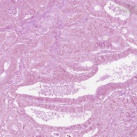
(a) Input

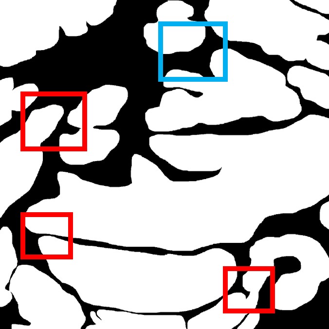
(b) GT

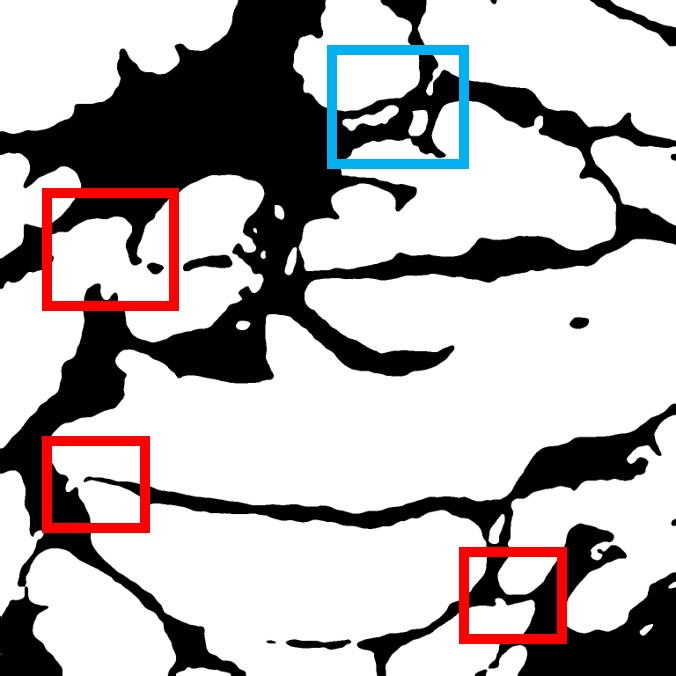
(c) XNet [65]

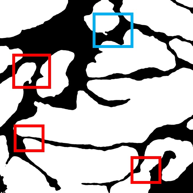
(d) Ours

Figure 1: Illustration of the significance of topological correctness in gland segmentation. (a) an input image. (b) ground truth GT. (c) the result of SoTA semi-supervised gland segmentation method [65] devoid of any topological regularization. (d) our segmentation result. For the regions within boxes, the SoTA’s result has errors that, while minor at the pixel level, significantly alter the semantic interpretation. The red boxes indicate prediction errors such as incorrect merging or separating adjacent glands, and the blue box indicates false positive gland predictions. These errors affect the pathologist’s decision and analysis.

Despite the success of existing semi-supervised segmentation methods, most of them focus on pixel-level accuracy and are error-prone with regard to the topology of the segmentation, i.e., the number of connected components and their spatial arrangement. See Fig. 1(c) for an illustration. The state-of-the-art (SoTA) semi-supervised method [65] still fails to properly maintain glands’ topological correctness, as highlighted by the boxed regions. Such topological errors can cause mistakenly merged/separated glands, significantly change their morphological measures (size, aspect ratio, etc), and consequently affect the downstream analysis/prediction. Similar issues may happen for nuclei segmentation tasks. This is indeed a very common issue. Both glands and nuclei are objects with similar appearances. Furthermore, they are often densely distributed within the tissue. If not addressed properly, these topological errors will significantly impact downstream analysis.

There are existing methods enforcing segmentation to have correct topology [19, 20, 44, 6, 18, 15, 53, 47]. These methods compare the predictions and ground truth (GT) in terms of their topology, using differentiable loss functions based on tools such as persistent homology [19, 6, 47], discrete Morse theory [20, 21, 16], homotopy warping [18], topological interactions [15], and centerline comparison [44, 53]. Despite the success of these topology-aware segmentation methods, they rely heavily on well-annotated, topologically correct labels, as well as the explicit topological information extracted from these labels. These methods are not suitable for a semi-supervised setting with limited annotations. Clough et al. [6] assume a fixed topology for input data and use a topology-preserving loss in a semi-supervised setting. However, their assumption is too strong and cannot adapt to pathology images, where at different locations we have different numbers of glands/nuclei. Our work aims to break such limitations by unearthing essential topological information from the vast amount of unlabeled images.

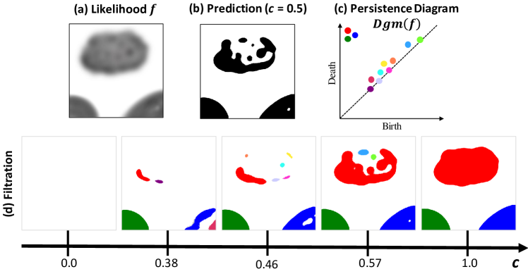
Figure 2: (a) A predicted likelihood map $f$, (b) the equivalent binary prediction, and (c) the corresponding persistence diagram $Dgm(f)$, which tends to be noisy. In (d), consider the filtration for different values of threshold $c$. Notice that there are three true, or signal, structures, denoted by colors red, green, and blue, which persist across the range of $c$. Hence the dots corresponding to these structures are located at the upper-left corner of $Dgm(f)$. The remaining colors denote several noisy structures which persist for a short range of $c$, and thus their dots appear closer to the diagonal. Note that we only show 0-dim persistent dots pertaining to connected components in $Dgm(f)$.

In this paper, we propose the first topology-aware solution for semi-supervised segmentation of pathology images. The method learns to segment with high accuracy in topology. The key challenge is to learn a robust representation of the topology from a large amount of unlabeled images. Inspired by the philosophy of consistency-learning methods, we propose to learn the representation by enforcing the consistency between different predictions in terms of topology. For unlabeled data, even though the true topology is unknown, for different perturbed inputs, a robust model should make predictions with consistent topology. In particular, we adopt the popular teacher-student framework, consisting of student and teacher models. A pixel-wise consistency loss is usually employed to force the two models to make consistent predictions at every pixel. Such a loss, however, does not guarantee topological correctness.

We introduce novel topology-aware losses to ensure the student and teacher models both make predictions with consistent topology. One may suggest directly applying existing topological losses [19, 20] to force the two predictions to have similar topology. However, these approaches will not work in practice. During the training, the outputs of both models are noisy and thus have a large amount of “noisy” structures (Fig. 2). These noisy structures will oscillate through training and significantly distract the learning from concentrating on the true topological signals.

To this end, we propose to decompose the topological structures of a prediction into signal topology and noise topology. This can be achieved by decomposing the topological features, formalized as the persistence diagram [10], into signal and noise. Fig. 3 illustrates this. We only enforce the signal topology of the teacher and the student’s prediction to be consistent. This is achieved by a signal topology consistency loss that matches the signal topological features using the Wasserstein distance [7, 8] between persistence diagrams. Meanwhile, for the noise topology, we introduce a noise topology removal loss, based on a theoretical measure called total persistence [8]. It aggregates the saliency of all noisy topological structures. Minimizing it essentially removes all these noisy topological structures. Combining the proposed signal topology consistency loss and noise topology removal loss with the classic pixel-wise consistency loss, our method achieves the desired goal and ensures both the student and the teacher learn the topological representation that is truly relevant.

In summary, our contribution is three-fold:

• We propose the first topology-aware method for semi-supervised segmentation of pathology images. The method learns to segment in a semi-supervised setting with high topological accuracy.

• To learn the robust representation of topology from the vast amount of unlabeled images, we propose a differentiable and continuous-valued topological consistency loss based on persistent homology. This regularization can be seamlessly integrated into any teacher-student framework, enabling the learning of topological representations through an end-to-end training process.

• To address the challenge of the noisy output of both teacher and student networks, we propose to decompose topological features into signal and noise. We propose novel losses to ensure consistency for signal topology and to remove noise topology.

Extensive experiments on three public pathology image datasets demonstrate the superiority of our method on both pixel- and topology-wise performance compared to other SoTA semi-supervised methods on two settings of $10\%$ and $20\%$ labeled data.

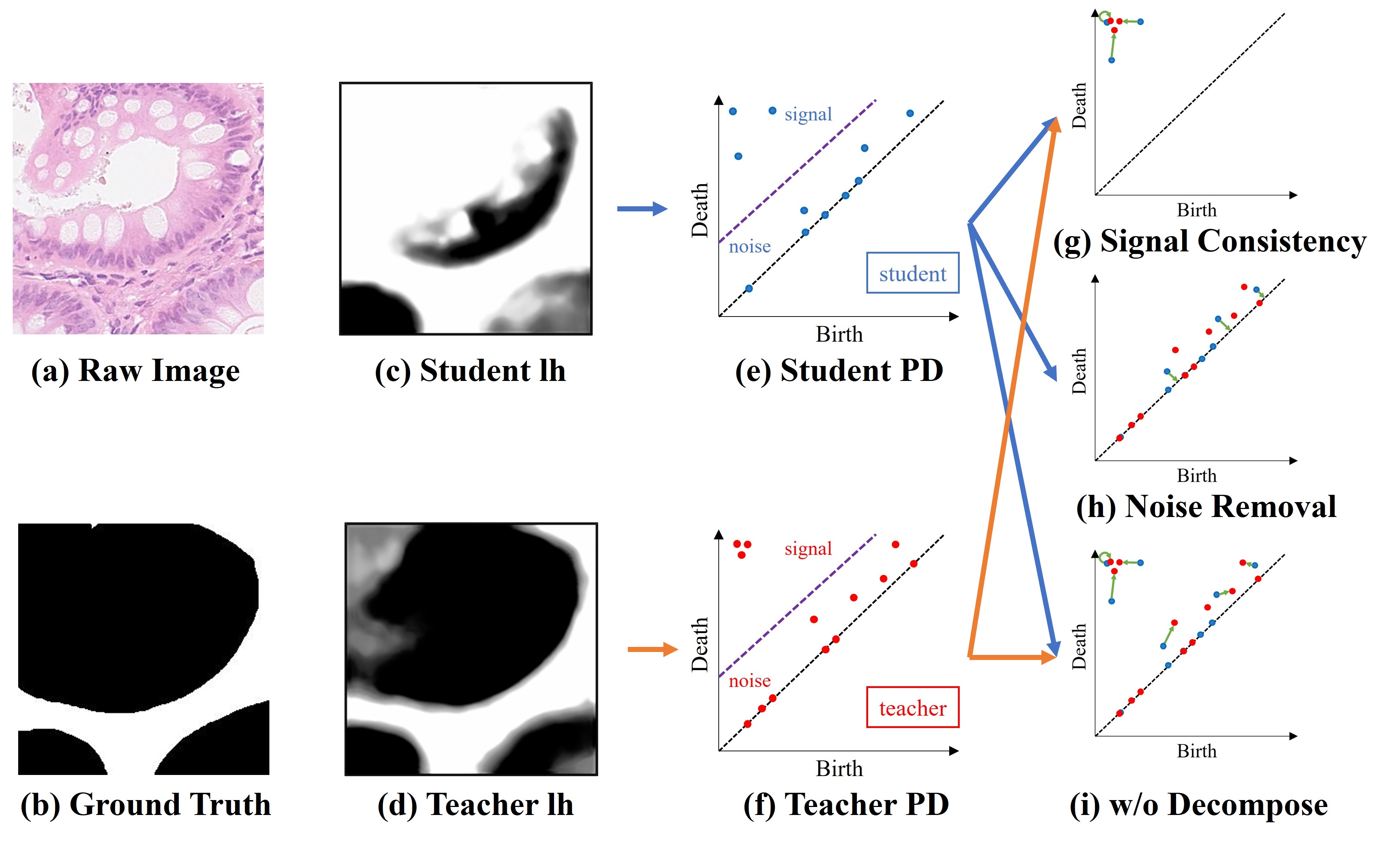
Figure 3: Inituition of our decomposition and matching strategy. (a) the raw image. (b) the ground truth, just for illustration. (c) the student likelihood (lh). (d) the teacher likelihood. (e) decomposition of the persistence diagram of student likelihood. The purple line demonstrates the decomposition. (f) decomposition of the persistence diagram (PD) of teacher likelihood. (g) the consistency between the signal topology. Green arrows show the matching process. (h) the noise topology removal process. (i) the matching process without decomposition.

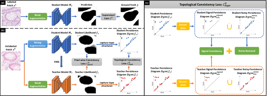
Figure 4: An overview of our method TopoSemiSeg. (a) denotes the labeled workflow. The student model is learned from labeled images via the supervised loss $\mathcal{L}^{S}$. (b) denotes the unlabeled workflow. The student model is learned from unlabeled images using $\mathcal{L}^{U}$, which consists of pixel-wise consistency loss $\mathcal{L}^{U}_{\text{pixel}}$ and topological consistency loss $\mathcal{L}^{U}_{\text{topo}}$. (c) shows the details of our proposed topological consistency loss, which encompasses our decomposition and optimal matching strategy, signal topology consistency loss $\mathcal{L}^{U}_{\text{topo-cons}}$ and noise topology removal loss $\mathcal{L}^{U}_{\text{topo-rem}}$.

2 Related Work

Segmentation with limited annotations. To address the scarcity of annotated data, semi-supervised learning (SemiSL) has emerged as a pivotal methodology in medical image segmentation [25]. The primary schemes in this domain encompass pseudo-labeling [58, 63, 42], consistency learning [22, 33, 40] and entropy minimization [55, 14, 2]. Pseudo-labeling-based methods aim to generate pseudo-labels for unlabeled data, which are then used to train the model further. To improve the quality of pseudo-labels, Wang et al. [54] propose a confidence-aware module to select pseudo labels with high confidence. Some works try to refine the pseudo-labels by morphological methods [50] or adding additional refinement networks [63, 43]. By learning better representations that pull similar samples together and push dissimilar ones apart, contrastive learning is also applied in SemiSL [59, 60, 1].

Another main scheme in SemiSL is consistency learning, which emphasizes consistent predictions under various perturbations. Different perturbations at input or feature level are proposed to compel the model to be robust [33, 34]. Also, most of these methods are the variants of Mean-Teacher framework [49], which encourages invariant predictions for perturbed inputs, like combining with uncertainty [61] and calculating different levels of consistency [35, 4]. However, most of the existing SemiSL methods based on consistency enforcement do not ensure topological correctness and cannot explicitly preserve the topological characteristics during the training, thus inevitably limiting the segmentation performance.

Topology-aware image segmentation. The integration of topological concepts into deep learning for image segmentation has recently attracted significant attention, aiming to leverage the robustness of topological features in segmentation tasks. Traditional image segmentation techniques primarily focus on pixel or region-based information, which may overlook the global structures and connectivity inherent within the images. Topology-aware segmentation methods, particularly those employing persistent homology and other topological data analysis (TDA) tools, have been introduced to address these limitations.

Persistent Homology [9] is one of the most popular tools in TDA and can capture the birth and death time of structures. As a pioneer work, Hu et al. [19] propose a topology-preserving loss function to enforce the predicted segmentation maps to have the same topology as the GT. Following this, many methods use different theories in TDA to improve topology, such as persistent homology [6, 47, 39, 17], homotopy warping [18], discrete Morse theory [20, 21, 16], topological interactions [15], and center-line transforms [44, 53].

Nevertheless, the above methods are all under a fully-supervised setting. Fine-grained structures require detailed annotations, which is time- and labor-intensive. Unlike previous methods, ours is the first to unearth topological information from the unlabeled data in a semi-supervised setting, reducing annotation effort and utilizing the structural information from unlabeled data more effectively.

3 Proposed Method

In this section, we first provide an overview of our proposed method TopoSemiSeg in Sec. 3.1. Then, we give a brief introduction to the background of persistent homology in Sec. 3.2. Finally, we introduce our topological regularization for the unsupervised setting in Sec. 3.3.

In SemiSL, we have a small set of labeled training samples and a much larger set of unlabeled samples. Let $\mathcal{D}_{L}=\{(x^{L}_{1},y_{1}),(x^{L}_{2},y_{2}),...,(x^{L}_{N_{L}},y_{N_{L}})\}$ be the dataset of $N_{L}$ labeled samples, and $\mathcal{D}_{U}=\{x^{U}_{1},x^{U}_{2},...,x^{U}_{N_{U}}\}$ be the unlabeled dataset of $N_{U}$ images, where $N_{L}<<N_{U}$. $x_{i}^{U}$ denotes the $i$-th unlabeled image and $x_{i}^{L}$ denotes the $i$-th labeled image with its corresponding pixel-wise label $y_{i}$.

The objective of SemiSL is to unearth the rich information within the unlabeled data, using limited guidance from labeled data. Most existing works only consider pixel-wise performance, ignoring the importance of topological correctness. Here, we take both of them into consideration.

3.1 Overview of the Method

Fig. 4 provides an overview of our method. We adopt the popular teacher-student framework [49] in SemiSL. This framework contains two networks – a student and a teacher – with identical architecture. We denote the student network as $M_{s}$, parameterized by $\theta_{s}$, and the teacher network as $M_{t}$, parameterized by $\theta_{t}$. The student network learns from the teacher network. It is trained by minimizing the supervised loss $\mathcal{L}^{S}$ on the labeled data and the unsupervised loss $\mathcal{L}^{U}$ on the unlabeled data. More details can be found in Fig. 4(a) and (b). The overall training objective is formulated as

$$\mathcal{L}=\mathcal{L}^{S}+\mathcal{L}^{U}$$ (1)

To make full use of limited annotations, $\mathcal{L}^{S}$ is defined as the combination of cross-entropy loss ($\ell_{CE}$) and Dice loss ($\ell_{Dice}$) [48] between the predictions and the labels:

$$\mathcal{L}^{S}(\mathcal{D}_{L},M_{s})$$ (2)

$$= \sum_{i=1}^{N_{L}}\left[\lambda^{L}_{1}\ell_{CE}(M_{s}(x_{i}^{L}),y_{i})+\lambda^{L}_{2}\ell_{Dice}(M_{s}(x_{i}^{L}),y_{i})\right]$$

where $\lambda^{L}_{1}$ and $\lambda^{L}_{2}$ are adjustable weights.

For unlabeled data, we apply strong augmentations $A_{strong}$ (resp., weak augmentations $A_{weak}$) and provide them to the student network (resp., the teacher network). The unsupervised loss enforces the consistency between predictions of the student and teacher models. It consists of two loss terms: pixel-wise consistency loss ($\mathcal{L}^{U}_{\text{pixel}}$) and the topological consistency loss $\mathcal{L}^{U}_{\text{topo}}$.

$$\mathcal{L}^{U}=\lambda^{U}_{1}\mathcal{L}^{U}_{\text{pixel}}+\lambda^{U}_{2}\mathcal{L}^{U}_{\text{topo}}$$ (3)

where $\lambda^{U}_{\ast}$ are adjustable weights.

We formulate the pixel-wise consistency loss as the cross-entropy (CE) loss between the outputs of the student and teacher models:

$$\mathcal{L}^{U}_{\text{pixel}}(\mathcal{D}_{U},M_{s},M_{t})$$ (4)

$$= \sum_{i=1}^{N_{U}}\ell_{CE}(M_{s}(A_{strong}(x_{i}^{U})),M_{t}(A_{weak}(x_{i}^{U})))$$

The topological consistency loss $\mathcal{L}^{U}_{\text{topo}}$ contains two topology-aware loss terms, $\mathcal{L}^{U}_{\text{topo-cons}}$ and $\mathcal{L}^{U}_{\text{topo-rem}}$,

$$\mathcal{L}^{U}_{\text{topo}}=\mathcal{L}^{U}_{\text{topo-cons}}+\mathcal{L}^{U}_{\text{topo-rem}}$$ (5)

which are crucial for learning a robust topological representation from unlabeled data. They will be explained in the next subsection.

During the training phase, the student network’s parameters $\theta_{s}$ are updated by minimizing the overall loss (Eq. 1). We update the teacher model’s parameters $\theta_{t}$ based on the student model’s parameters using exponential moving average (EMA) [49]. In particular, at the $(\tau+1)^{\text{th}}$ epoch, the $\theta_{t}$ is updated as $\theta_{t}(\tau+1)=\alpha\theta_{t}(\tau)+(1-\alpha)\theta_{s}(\tau+1)$ where $\alpha$ is the EMA decay controlling the updating rate.

3.2 Background: Persistent Homology

In algebraic topology [38], homology classes account for topological structures in all dimensions. 0-, 1-, and 2-dimensional structures describe connected components, loops/holes, and cavities/voids, respectively. For binary images, the number of $d$-dimensional topological structures is called the $d$-dimensional Betti number, $\beta_{d}$. Despite the well-understood topological space for a binary image, the theory does not directly extend to real-world scenarios with continuous, noisy data. For example, in image analysis, we need a principled tool to reason about the topology from a continuous likelihood map. To bridge this gap, the theory of persistent homology was invented in the early 2000s [9].

Persistent homology has emerged as a powerful tool for analyzing the topology of various kinds of real-world data, including images. In the image segmentation task, we apply persistent homology to the likelihood map of a deep neural network to reason about its topology. Given an image in the 2D domain $I\subseteq\mathbb{R}^{2}$, we use a network to generate a likelihood map $f$. The segmentation map is obtained by thresholding $f$ at a certain threshold $c$ (usually $0.5$). We define a sublevel set: $S_{c}:=\{(m,n)\in I\>|\>f(m,n)\leq c\}$. With all different threshold values sorted in an increasing order ($c_{1}<c_{2}<\cdots<c_{n}$), we obtain a filtration, i.e., a series of growing sublevel sets: $\varnothing\subseteq S_{c_{1}}\subseteq S_{c_{2}}\subseteq...\subseteq S_{c_{n}}=I$. As the threshold $c$ increases, topology of the sublevel set changes. New topological structures appear while old ones disappear. Persistent homology tracks the evolution of all topological structures, such as connected components and loops. All the topological structures and their birth/death times are captured in a so-called persistence diagram, providing a multi-scale topological representation (See Fig. 2).

A persistence diagram (PD) consists of multiple dots in a 2-dimensional plane. These dots are called persistent dots. Given a continuous-valued likelihood map function $f$, we have its persistence diagram $Dgm(f)$. Each persistent dot $p\in Dgm(f)$ represents a topological structure. Its two coordinates denote the birth and death filtration values for the corresponding topological structure, i.e., $p=(b,d)$, where $b=birth(p)$ and $d=death(p)$. We can calculate the persistent diagrams for outputs of both the student and the teacher models, in order to compare the two likelihood maps from a topological perspective.

3.3 Topological Consistency Loss

We propose topological consistency loss to ensure the teacher and student models make consistent predictions in terms of topology. Given the likelihood maps of both teacher and student models, $f_{t}$ and $f_{s}$, we first compute the persistence diagrams, $Dgm(f_{t})$ and $Dgm(f_{s})$. However, directly comparing the two diagrams is not desirable. As shown in Fig. 3, without supervision, not only the student persistence diagram, but also the teacher persistence diagram are quite noisy. Direct comparison of the two diagrams can create a lot of unnecessary matching between noisy structures. This will cause inefficiency in learning, and can potentially even derail the whole training.

To address this challenge, we propose to decompose $Dgm(f_{s})$ and $Dgm(f_{t})$ into signal and noise parts. The signal part is used to enforce teacher-student consistency via a signal topology consistency loss. The noise part will be removed through a novel noise topology removal loss.

Signal-Noise Decomposition of a Persistence Diagram. We would like to decompose a diagram into signal and noise parts. However, in reality, without ground truth, the decomposition cannot be guaranteed to be accurate. Hence, we use the classic measure of persistence to decide whether a dot is a signal or noise.

For a persistent dot $p\in Dgm(f)$, its persistence is simply its life span, i.e., the difference between its death and birth time: $per(p)=death(p)-birth(p)$. Persistence is a good heuristic approximating the significance of a topological structure; the greater the persistence, the longer the structure exists through filtration, and the more likely the structure is a true signal. This is theoretically justified. The celebrated stability theorem [7, 8] implies that low-persistence dots are much easier to be “shed off” through perturbation of the input function $f$.

Formally, using a predetermined threshold $\phi$, we decompose $Dgm(f)$ into disjoint signal and noise persistence diagrams based on the persistence:

$$Dgm(f) =Dgm(f)^{signal}\dot{\bigcup}Dgm(f)^{noise}$$

$$Dgm(f)^{signal} =\{p\in Dgm(f)\>|\>per(p)>\phi\}$$

$$Dgm(f)^{noise} =\{p\in Dgm(f)\>|\>per(p)\leq\phi\}$$

where $\dot{\bigcup}$ denotes the disjoint union. We apply the same decomposition to both teacher and student model outputs, acquiring their signal and noise parts respectively.

$$Dgm(f_{s}) =Dgm_{stu}^{signal}\dot{\bigcup}Dgm_{stu}^{noise}$$

$$Dgm(f_{t}) =Dgm_{tea}^{signal}\dot{\bigcup}Dgm_{tea}^{noise}$$

The threshold $\phi$ is tuned empirically. These signal/noise diagrams for teacher/student output will be used for the two topology-aware losses introduced in Eq. 5.

Signal Topology Consistency Loss. After the decomposition of both persistence diagrams, we obtain $Dgm_{stu}^{signal}$ and $Dgm_{tea}^{signal}$ representing the meaningful topological signals. Our first topology-aware loss is to ensure the two signal diagrams are the same. Similar to previous topological losses [19], we will use the classic Wasserstein distance between the two diagrams. Note: for any diagram $Dgm(g)$, we regard it as the generalized persistence diagram.

Definition 1 (Wasserstein distance between PDs [8]).

Given two diagrams $Dgm(g)$ and $Dgm(h)$, the $p$-th Wasserstein distance between them is defined as:

$$W_{p}(Dgm(g),Dgm(h))=\left(\underset{\gamma\in\Gamma}{inf}\sum\limits_{x\in Dgm(g)}{||x-\gamma(x)||}^{p}\right)^{\frac{1}{p}}$$

where $\Gamma$ represents all bijections from $Dgm(g)$ to $Dgm(h)$.

See Fig. 3(g) and (h) for an illustration. The Wasserstein distance essentially finds an optimal matching between dots of the two diagrams. Unmatched dots are matched to their projection on the diagonal line. The distance is computed by aggregating over distance between all the matched pairs of dots. The optimal matching, as well as the distance, can be computed using either the classic Hungarian method, or more advanced algorithms [31, 29].

Next, we write the signal topology consistency loss in terms of the student’s likelihood map, $f_{s}$. Denote by $\gamma^{*}$ the optimal matching between $Dgm_{stu}^{signal}$ and $Dgm_{tea}^{signal}$. Each student persistent dot $p_{stu}^{signal}\in Dgm_{stu}^{signal}$ is matched to either a teacher persistent dot, or its projection on the diagonal. We can now formulate our signal topology consistency loss $\mathcal{L}_{\text{topo-cons}}^{U}$ as squared distance between every student signal dot and its match:

$$\mathcal{L}_{\text{topo-cons}}^{U}=\sum\limits_{p\in Dgm_{stu}^{signal}}||p-\gamma^{\ast}(p)||^{2}$$ (6)

We still have to write the loss in terms of the student likelihood map. Note that in persistent homology, the birth and death times of every persistent dot are the function values of certain critical points. See Supplementary for more details and illustrations. For each 0-dimensional persistent dot $p$ in a student diagram, the birth is at a local maxima $x^{b}_{p}$ and the death is at a saddle point $x^{d}_{p}$, formally, $birth(p)=f_{s}(x^{b}_{p})$ and $death(p)=f_{s}(x^{d}_{p})$. Substituting into Eq. 6, we have

$$\mathcal{L}_{\text{topo-cons}}^{U}(f_{s})=\sum\limits_{p\in Dgm_{stu}^{signal}}\{[f_{s}(x^{b}_{p})-birth(\gamma^{\ast}(p))]^{2}\\ +[f_{s}(x^{d}_{p})-death(\gamma^{\ast}(p))]^{2}\}$$ (7)

which can be optimized with regard to the student network.

Noise Topology Removal Loss. So far, we have introduced how to decompose the diagram and how the signal part of the diagrams can be used to enforce topological consistency. We also introduce a loss to remove the noise topology from the student likelihood map. This turns out to be very powerful in practice: by removing the topological noise, we can stabilize the output of student network, and eventually also stabilize the teacher network via EMA.

Our noise topology removal loss is based on the concept of Total Persistence, which essentially measures the total amount of information a diagram carries. By minimizing the total persistence of the noise diagram, we are effectively removing all noise dots.

Definition 2 (Total Persistence [8]).

Given a persistence diagram, $Dgm(g)$, the $p$-th total persistence is :

$$P_{total}(Dgm(g))=\left(\sum\limits_{x\in Dgm(g)}\|x\|^{p}\right)^{\frac{1}{p}}$$ (8)

Similar to the consistency loss, we can define the loss in terms of the student likelihood map as follows:

$$\mathcal{L}_{\text{topo-rem}}^{U}(f_{s})=\sum\limits_{p\in Dgm_{stu}^{noise}}\left[f_{s}(x^{b}_{p})-f_{s}(x^{d}_{p})\right]^{2}$$ (9)

Differentiability of the Topology-Aware Losses. Both $\mathcal{L}_{\text{topo-cons}}^{U}$ and $\mathcal{L}_{\text{topo-rem}}^{U}$ are differentiable, as Eq. 7 and Eq. 9 are both written as polynomials of the likelihood map $f_{s}$ at certain critical pixels. Here it is crucial to assume the critical pixels, $x_{p}^{b}$ and $x_{p}^{d}$, remain constant locally. This is because the likelihood map is a piecewise linear function determined by the function values at a discrete set of pixel locations. Assuming without loss of generality that all pixels have distinct values, we can show that within a small neighborhood of the likelihood $f_{s}$, the order of all pixels in $f_{s}$ remains the same. Therefore, the algorithmic computation of persistence homology will associate the same set of critical pixels with each persistence dot $x$ in the diagram. In other words, we can assume $x_{p}^{b}$ and $x_{p}^{d}$ remain constant.

Dataset	Labeled Ratio (%)	Method	Pixel-Wise				Topology-Wise
			Accuracy $\uparrow$	Dice_Obj $\uparrow$	IoU $\uparrow$		Betti Error $\downarrow$	Betti Matching Error $\downarrow$	VOI    $\downarrow$
CRAG	10%	MT [49]	0.862	0.821	0.713		2.238	62.250	0.977
		EM [51]	0.834	0.789	0.688		2.178	80.100	1.027
		UA-MT [61]	0.874	0.837	0.728		1.703	66.450	0.947
		HCE* [26]	0.891	0.862	0.773		1.286	35.530	0.861
		URPC [35]	0.872	0.829	0.728		1.732	74.600	0.883
		XNet [65]	0.895	0.872	0.781		0.578	15.050	0.773
		TopoSemiSeg	0.905	0.884	0.798		0.227	10.475	0.758
	20%	MT [49]	0.887	0.858	0.759		2.603	99.025	0.867
		EM [51]	0.903	0.869	0.776		1.933	75.225	0.798
		UA-MT [61]	0.895	0.859	0.765		1.822	70.850	0.829
		HCE* [26]	0.910	0.881	0.809		0.875	17.400	0.769
		URPC [35]	0.881	0.849	0.744		2.489	99.500	0.912
		XNet [65]	0.907	0.883	0.792		0.422	10.900	0.735
		TopoSemiSeg	0.912	0.898	0.820		0.226	8.575	0.709
	100%	Fully-supervised	0.945	0.928	0.869		0.149	5.650	0.547
GlaS	10%	MT [49]	0.815	0.790	0.671		2.392	31.125	1.079
		EM [51]	0.833	0.819	0.708		1.431	19.188	1.051
		UA-MT [61]	0.728	0.845	0.829		2.086	26.650	1.018
		HCE* [26]	0.859	0.852	0.762		0.631	11.950	0.953
		URPC [35]	0.829	0.849	0.751		1.155	19.588	0.968
		XNet [65]	0.871	0.874	0.786		0.843	14.238	0.917
		TopoSemiSeg	0.890	0.878	0.797		0.551	8.300	0.811
	20%	MT [49]	0.870	0.863	0.771		2.126	29.963	0.925
		EM [51]	0.861	0.865	0.776		1.255	17.275	0.841
		UA-MT [61]	0.874	0.866	0.781		1.123	18.038	0.869
		HCE* [26]	0.864	0.871	0.779		0.871	16.213	0.824
		URPC [35]	0.876	0.878	0.794		0.759	14.350	0.837
		XNet [65]	0.886	0.884	0.804		0.735	10.188	0.816
		TopoSemiSeg	0.896	0.895	0.818		0.510	9.825	0.808
	100%	Fully-supervised	0.920	0.917	0.853		0.473	7.125	0.686
MoNuSeg	10%	MT [49]	0.889	0.748	0.607		10.210	292.857	0.874
		EM [51]	0.901	0.757	0.612		10.339	257.071	0.844
		UA-MT [61]	0.898	0.741	0.594		10.227	255.428	0.862
		HCE* [26]	0.882	0.761	0.617		14.210	377.928	0.890
		CCT [40]	0.892	0.766	0.624		8.063	225.500	0.839
		URPC [35]	0.896	0.774	0.633		6.829	214.428	0.863
		TopoSemiSeg	0.909	0.783	0.646		6.661	196.357	0.789
	20%	MT [49]	0.896	0.767	0.624		12.522	246.786	0.873
		EM [51]	0.905	0.777	0.637		7.160	198.571	0.805
		UA-MT [61]	0.904	0.772	0.632		9.406	246.857	0.826
		HCE* [26]	0.899	0.771	0.642		13.330	311.143	0.829
		CCT [40]	0.903	0.785	0.648		7.977	207.857	0.832
		URPC [35]	0.909	0.779	0.639		5.325	193.429	0.788
		TopoSemiSeg	0.908	0.793	0.653		4.250	188.642	0.787
	100%	Fully-supervised	0.929	0.817	0.702		2.491	142.429	0.657

Table 1: Quantitative results on three pathology image datasets. We compare our method with several state-of-the-art semi-supervised medical image segmentation methods on two settings of $10\%$ and $20\%$ labeled data. The best results are highlighted in bold, and * indicates that the method is re-implemented by ourselves

4 Experiments

We conduct extensive experiments on three public and widely used pathology image datasets. We compare our method against SoTA semi-supervised segmentation methods on both pixel- and topology-wise evaluation metrics. Implementation details are in the Supplementary.

Datasets. We evaluate our proposed method on Colorectal Adenocarcinoma Gland (CRAG) [13], Gland Segmentation in Colon Histology Images Challenge (GlaS) [45], and Multi-Organ Nuclei Segmentation (MoNuSeg) [30]. More details are provided in the Supplementary.

Evaluation Metrics. We select three widely used pixel-wise evaluation metrics, Object-level Dice coefficient (Dice_Obj) [57], Intersection over Union (IoU) and Pixel-wise accuracy. Topology-relevant metrics mainly measure structural accuracy. We also select three topological evaluation metrics, Betti Error, Betti Matching Error [47], and Variation of Information (VOI) [36]. More details are provided in the Supplementary.

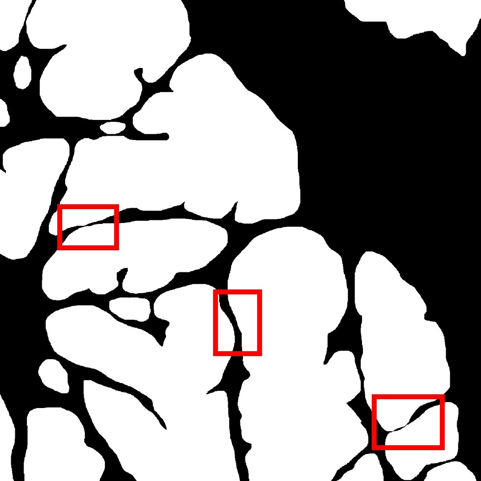
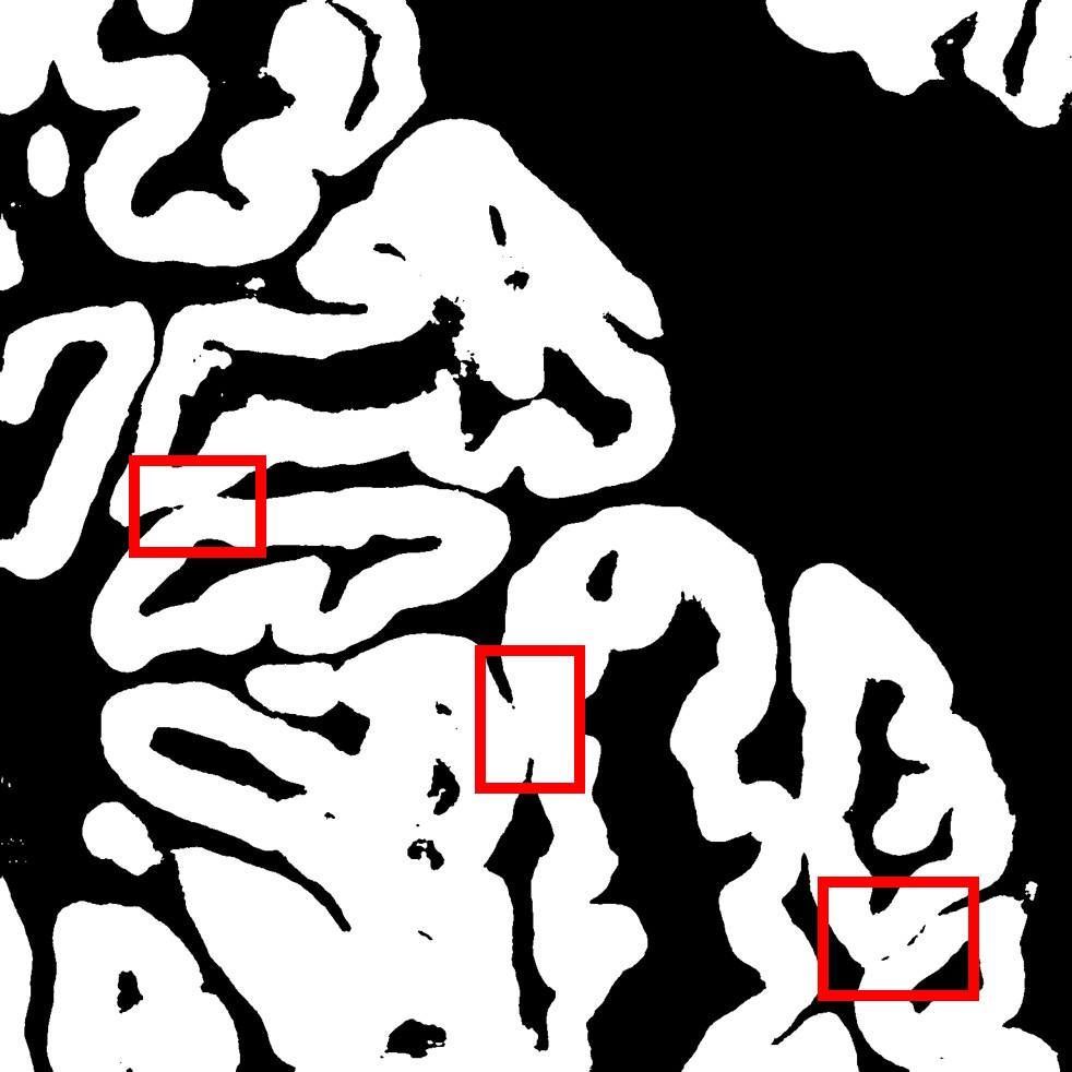
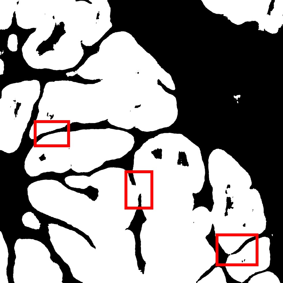
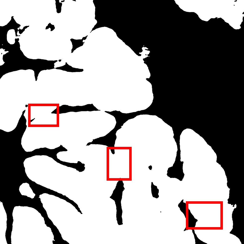
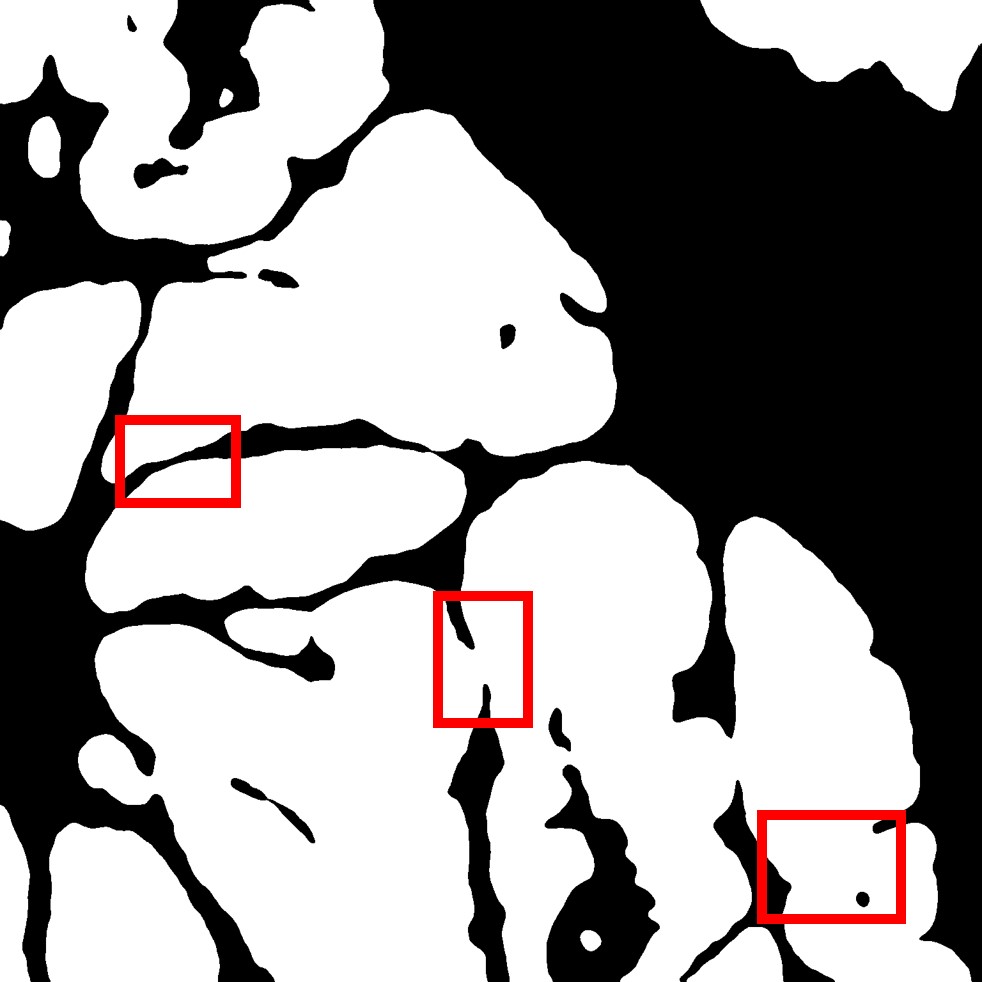
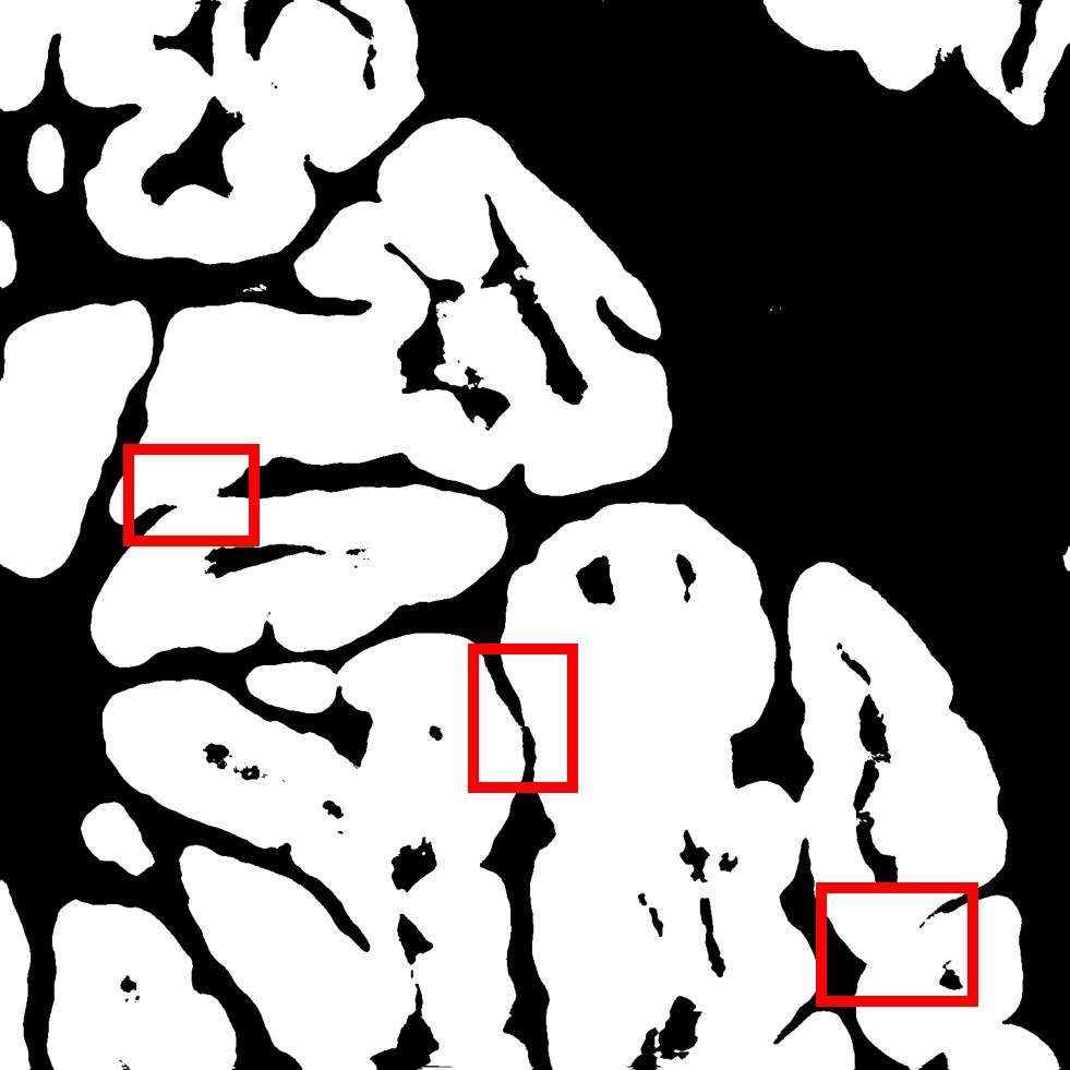
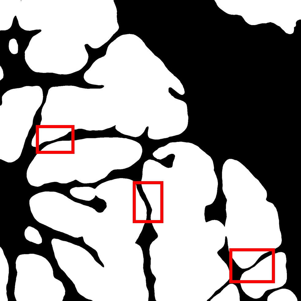
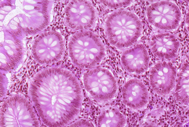
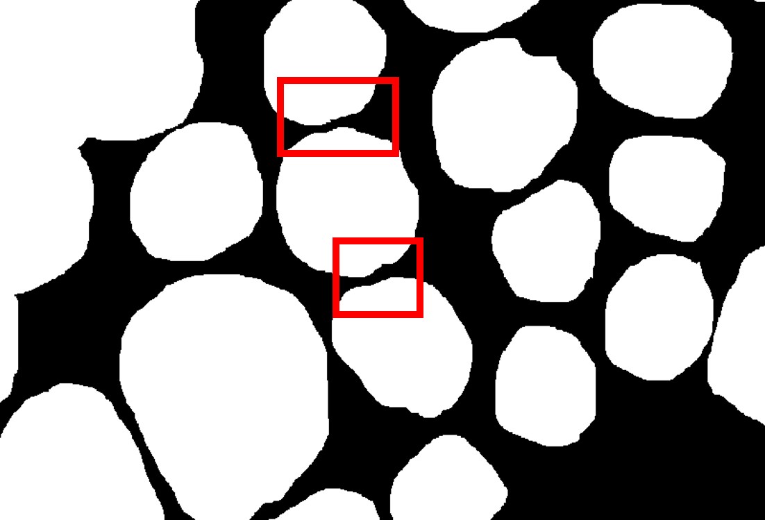
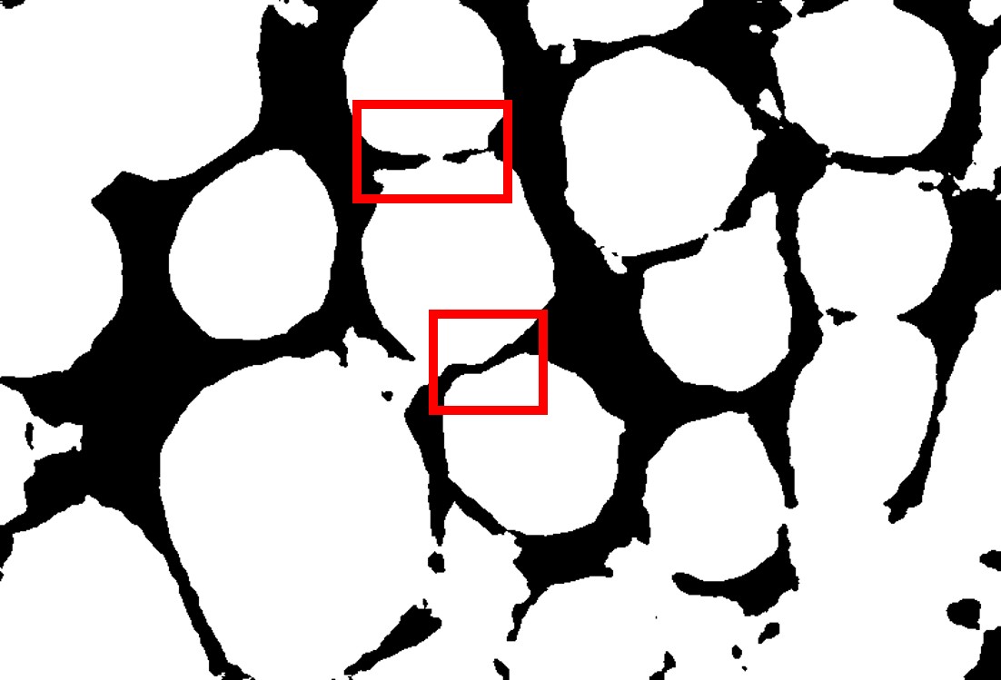
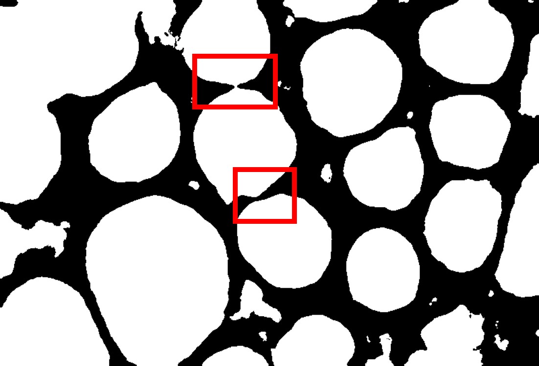
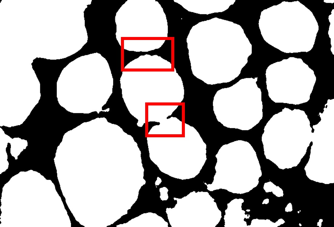
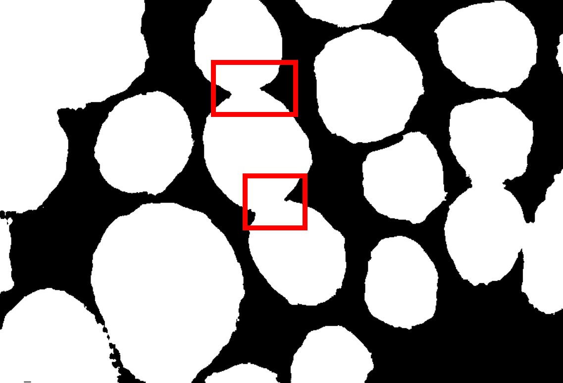
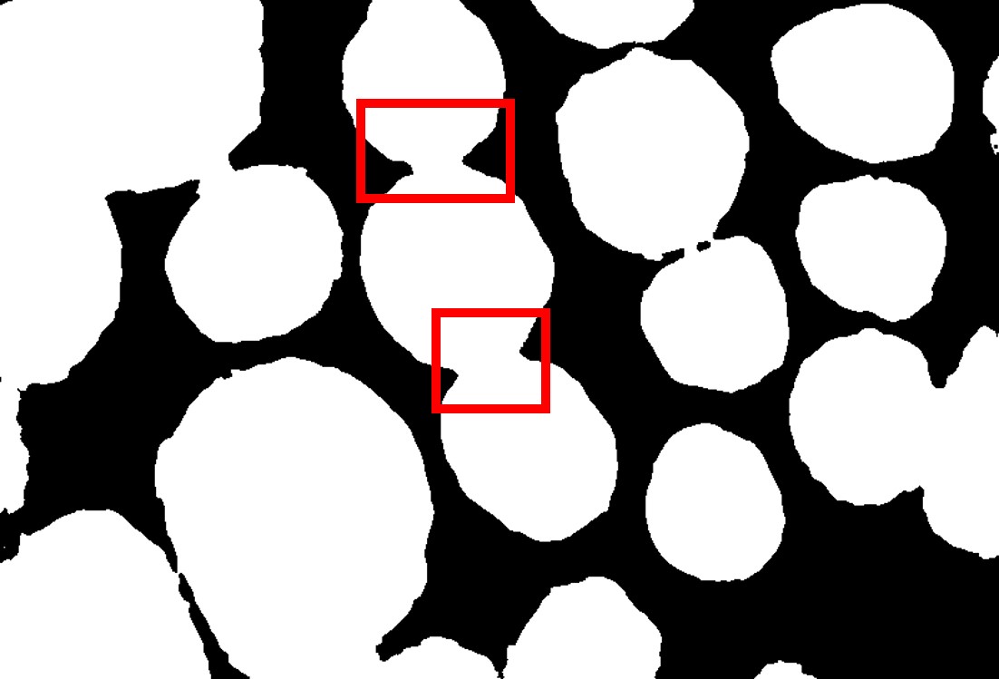
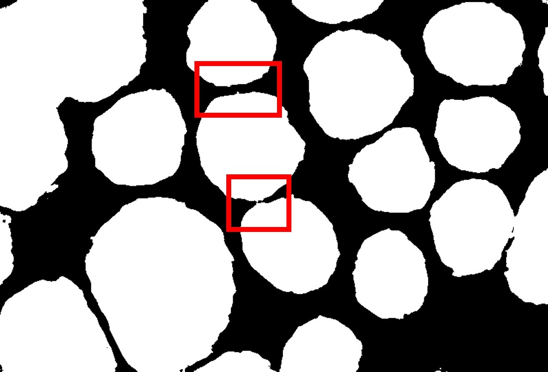
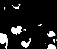
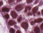
(a) Raw Image

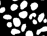
(b) Ground Truth

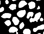
(c) MT

(d) EM

(e) UA-MT

(f) HCE

(g) URPC

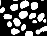
(h) Ours

Figure 5: Qualitative results on three pathology image datasets using $20\%$ labeled data for training. Locations prone to topological errors are shown within red boxes. Row 1: CRAG, Row 2: GlaS, Rows 3 & 4: MoNuSeg. Zoom in for better views.

4.1 Results: Comparison with SoTA SemiSL

We conduct experiments on different fractions of labeled data, specifically, $10\%$ and $20\%$. Training UNet++ [66] on $100\%$ of the labeled data is treated as the performance upper bound. To indicate the effectiveness and superiority of our method, we select several SoTA semi-supervised methods for comparison both from pixel and topological perspectives. Quantitative results are shown in Tab. 1, and qualitative results are shown in Fig. 5. We discuss more below.

Quantitative Results. For a comprehensive comparison, we select several classical and recent SoTA SemiSL methods like MT [49], EM [51], UA-MT [61], HCE [26], URPC [35], XNet [65] and CCT [40]. Note that HCE is re-implemented by ourselves due to code unavailability. As shown in Tab. 1, our method not only achieves comparable performance on pixel-wise evaluation metrics but also achieves the best results on all topology-wise metrics. This indicates that our proposed TopoSemiSeg is able to unearth and utilize topological information in unlabeled data well, without too much sacrifice on pixel-level performance.

Qualitative Results. In Fig. 5, we provide the qualitative results of the methods on $20\%$ labeled data for each dataset. Compared to other SoTA SemiSL methods, our method does better where topological errors are prone to occur, as shown in the red boxes. The proposed TopoSemiSeg ensures topological integrity: by enforcing signal consistency, we can maintain the thin separation between the densely distributed glands and cells. Additionally, the noise removal component of our loss minimizes the occurrence of false positive cells, as can be seen in Row 3. This is in contrast to the results obtained from the other baseline methods, which contain a discernible presence of noise and unoccupied interspaces in and around the glandular and cellular structures. Our method can effectively address and rectify these issues. This is due to the fact that we not only focus on the signal topology which should be preserved, but also remove all the noise topology during training, thus making the model learn more robust and accurate topological representations from the unlabeled data.

4.2 Ablation Studies

We conduct experiments to illustrate the effectiveness and robustness of our hyper-parameters and experimental settings. All experiments are performed on the CRAG dataset using $20\%$ labeled data.

Weight of Topological Consistency Loss $\lambda^{U}_{2}$. We study the effect of the weight of the topological consistency loss $\lambda^{U}_{2}$ introduced in Eq. 3. As shown in Tab. 2, at $\lambda^{U}_{2}=0.002$, the model achieves the best Object-level Dice coefficient, Betti Matching Error, and VOI. Additionally, a reasonable range of $\lambda^{U}_{2}$ always results in improvement. This demonstrates the efficacy and robustness of the proposed method.

$\lambda^{U}_{2}$	Pixel-Wise		Topology-Wise
	Dice_Obj $\uparrow$		Betti Error $\downarrow$	Betti Matching Error $\downarrow$	VOI $\downarrow$
0	0.887		0.230	10.525	0.783
0.001	0.874		0.217	12.175	0.736
0.002	0.898		0.226	8.575	0.709
0.005	0.889		0.213	9.875	0.739
0.008	0.896		0.235	9.700	0.722
0.01	0.873		0.277	9.725	0.754

Table 2: Ablation study on loss weight $\lambda^{U}_{2}$

Robustness of Persistence Threshold $\phi$. In order to compute the topological consistency loss, we define a persistence threshold $\phi$ to decompose both the persistence diagrams into signal and noise parts. We conduct experiments on different values of $\phi$. As we can see from Tab. 3, our method is not sensitive to the value of $\phi$ and a wide range of $\phi$ (from $0.5$ to $0.9$) results in improvements on topological metrics. This demonstrates the robustness of our method with respect to perturbations.

$\phi$	Pixel-Wise		Topology-Wise
	Dice_Obj $\uparrow$		Betti Error $\downarrow$	Betti Matching Error $\downarrow$	VOI $\downarrow$
0	0.887		0.230	10.525	0.783
0.50	0.881		0.241	8.950	0.753
0.60	0.895		0.219	9.600	0.725
0.70	0.898		0.226	8.575	0.709
0.80	0.896		0.209	9.000	0.722
0.90	0.889		0.231	10.150	0.717

Table 3: Ablation study on persistence threshold $\phi$

Generalizability to Different Backbones. We verify the generalizability of our method by performing experiments on three different backbones, UNet [41], PSPNet [64], and DeepLabV3+ [5], keeping the same values of hyper-parameters for each. Tab. 4 shows that our method is robust to backbone selections and can obtain performance improvements with each of them. For those with poor topological performances, like PSPNet [64], our method significantly reduces the number of topological errors. This proves the effectiveness and generalizability of our method in that it can facilitate capturing topological information from the unlabeled data irrespective of the backbone.

Method	Pixel-Wise		Topology-Wise
	Dice_Obj$\uparrow$		BE$\downarrow$	BME$\downarrow$	VOI$\downarrow$
UNet [41]	0.892		0.266	10.775	0.790
UNet [41]+Ours	0.893		0.236	8.700	0.722
PSPNet [64]	0.773		1.809	70.625	1.337
PSPNet [64]+Ours	0.775		1.021	44.150	1.040
DeepLabV3+ [5]	0.883		0.293	14.000	0.725
DeepLabV3+ [5]+Ours	0.891		0.265	11.725	0.713
UNet++ [66]	0.887		0.230	10.525	0.783
UNet++ [66]+Ours	0.898		0.226	8.575	0.709

Table 4: Comparison on different backbones. BE and BME respectively denote Betti Error and Betti Matching Error.

5 Conclusion

This work introduces TopoSemiSeg, the first semi-supervised method that learns topological representation from unlabeled data for pathology image segmentation. It consists of a novel and differentiable topological consistency loss integrated into the teacher-student framework. We propose to decompose the calculated persistence diagrams into true signal and noise components, and respectively formulate signal consistency and noise removal losses from them. These losses enforce the model to learn a robust representation of topology from unlabeled data and can be incorporated into any variant of the teacher-student framework. Extensive experiments on several pathology image datasets indicate that our TopoSemiSeg consistently outperforms other SoTA semi-supervised methods.

TopoSemiSeg: Enforcing Topological Consistency for Semi-Supervised Segmentation of Histopathology Images
— Supplementary Material —

In the supplementary material, we begin with notations for foreground and background in Sec. 6, followed by a description of the correspondence between persistence dots and the likelihood map in Sec. 7. Next, we provide detailed descriptions of the datasets in Sec. 8, followed by implementation details in Sec. 9. We also provide the reference of our baselines in Sec. 10. In Sec. 11, we describe the evaluation metrics in detail. More qualitative results are given in Sec. 12. Finally, to further demonstrate the effectiveness of our proposed method, the ablation study on fully supervised topological loss and topological consistency loss is provided in Sec. 13.

6 Notes on Foreground and Background

Here, we provide some notations about foreground and background in our paper. Our algorithm uses black as the foreground and white as the background as can be seen in Fig. 2- Fig. 4 of the main paper and Fig. 6 of the Supplementary. For better visualization, however, we display the segmentation results and ground truth with white as the foreground in Fig. 1 and Fig. 5 of the main paper and Fig. 7 of the Supplementary.

7 Mapping Persistent Dots to the Likelihood

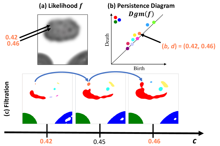
Figure 6: (a) A predicted likelihood map $f$, and (b) the corresponding persistence diagram $Dgm(f)$. Consider the orange persistent dot having birth $b$ and death $d$ times as $(b,d)=(0.42,0.46)$. We show the corresponding filtration in (c) for these specific birth/death times. At birth $b=0.42$, the connected component corresponding to the orange is born. At death $d=0.46$, this connected component dies as it gets absorbed into the older red connected component. Note that we only show 0-dim persistent dots pertaining to connected components in $Dgm(f)$.

In Fig. 6, we show how persistent dots in the persistent diagram can ultimately be mapped to pixels/voxels in the likelihood map. Consequently, the loss functions defined in Eq. 6- Eq. 7 of the main paper are differentiable: the penalty applied to the persistent dots is ultimately a penalty on the pixels/voxels of the likelihood. Hence backpropagation can take place: our proposed losses are differentiable.

In Fig. 6, we give an example of a likelihood $f$ in Fig. 6(a), and focus on the orange persistent dot in Fig. 6(b); let us call it $p$. It’s coordinate in the persistence diagram $Dgm(f)$ is nothing but its birth $b$ and death $d$ given by $(b,d)=(0.42,0.46)$.

There are precisely two pixels in the likelihood that capture the lifetime of this persistent dot $p$. We call them critical pixels. We denote the location of these critical pixels in $f$ using black arrows in Fig. 6(a). These two critical pixels have the values $0.42$ and $0.46$ respectively. We now map the likelihood to the persistence diagram below.

In the filtration Fig. 6(c), when the threshold is $0.42$, the critical pixel of the same value gets included into the binary map. It is a connected component on its own and is denoted by orange in Fig. 6(c) when $c=0.42$. This marks the birth of the connected component corresponding to the persistent dot $p$. At threshold $c=0.45$, we see this orange connected component grow larger as more pixels get introduced into the binary map. Finally, at $c=0.46$, the second critical pixel is introduced which joins the orange connected component to the older red connected component. This marks the death of the connected component corresponding to $p$ as it gets absorbed into the older red connected component. Hence, the persistent dot $p\in Dgm(f)$’s birth and death values each correspond to a single pixel location in the likelihood $f$.

Now, this persistent dot gets matched to the diagonal according to the bijection $\gamma^{*}$ introduced in Sec. 3.3. Consequently, the loss described in Eq. 6 pushes $p$ towards the diagonal. This means $p$ is a noisy structure and we would like to suppress/remove it. On pushing it to the diagonal, we force the birth and death times to be the same: the moment this structure is born, it should be automatically included in the older connected component. Hence it ceases to exist as a standalone connected component across any and all filtration values and is thus effectively removed as noise.

8 Details of the Datasets

1. Colorectal Adenocarcinoma Gland (CRAG) [13] is a collection of $213$ H&E stained colorectal adenocarcinoma image tiles captured at $20\times$ magnification, with full instance-level annotation. Most of the images are of the size $1512\times 1516$. It is officially divided into a training set with 173 samples and a test set with 40 samples. In our experiments, we separate the training set into $153$ images for training and $20$ images for validation. For $10\%$ and $20\%$ labeled data splitting, we randomly select $16$ and $31$ images with labels respectively, for training.

2. Gland Segmentation in Colon Histology Images Challenge (GlaS) is introduced in [45] and comprises of $165$ images derived from 16 H&E stained histological sections of stage T$3$ or T$4$ colorectal adenocarcinoma. The dataset is officially separated into a training set with $85$ samples and a test set with $80$ samples. In our experiments, we divide the training set into $68$ images for training and $17$ images for validation. For $10\%$ and $20\%$ labeled data splitting, we randomly select $7$ and $14$ images with labels for training.

3. Multi-Organ Nuclei Segmentation (MoNuSeg) [30] contains $44$ H&E stained images of size $1000\times 1000$ from seven organs. It consists of two sets, $30$ images containing $21,623$ nuclei for training and $14$ images for testing. In our experiments, we choose $20\%$ training data ($6$ images) as the validation set, and for $10\%$ and $20\%$ labeled data splitting, we randomly select $3$ and $5$ images with labels respectively for training.

9 Implementation Details

We train our model in two stages. The first stage is pre-training, using only $\mathcal{L}^{S}$ and $\mathcal{L}^{U}_{pixel}$ to train the network for several iterations. For CRAG and GlaS, we pre-train the model for $12000$ iterations; for MoNuSeg, we pre-train the model for $2000$ iterations. The second stage is fine-tuning using our topological consistency loss. We fine-tune the model for $500$ epochs using Eq. 1 as the overall training objective. While training, we use UNet++ [66] as our backbone for both student and teacher networks, and we adopt the Adam optimizer solver to train the model. The proposed algorithm is implemented on the PyTorch platform. The training hyper-parameters are set as follows: for CRAG and GlaS, the batch size is $16$, and the learning rate is $5e-4$. For MoNuSeg, the batch size is $8$, and the learning rate is $1e-4$. We first apply random cropping on both labeled and unlabeled data. The cropping size is $256\times 256$ for CRAG and GlaS and $416\times 416$ for MoNuSeg. After random cropping, we apply random rotation and flipping for weak augmentations, and for strong augmentations, we apply color change and morphological shift. The EMA decay rate $\alpha$ and $\lambda^{U}_{2}$ are set to $0.999$ and $0.002$ respectively. Introduced in [33], the weight factor of pixel-wise consistency loss is calculated by the Gaussian ramp-up function $\lambda^{U}_{1}=k*e^{-5*(1-\frac{\tau}{T})^{2}}$, where $k=0.1$ and $T$ is the total number of iterations. $\lambda_{1}^{L}$ and $\lambda_{2}^{L}$ in $\mathcal{L}^{S}$ are all set to $0.5$. The persistence threshold $\phi$ for decomposing the persistence diagrams is $0.7$. All the experiments are conducted on an NVIDIA RTX $A6000$ GPU with $48$ GB RAM.

10 Baseline Reference

In our experiments, some baselines are based on the implementations of others. Here, we provide our baselines’ source for reference and appreciate their efforts on the public code.

MT [49], EM [51], UA-MT [61], and URPC [35] are based on the implementations from: https://github.com/HiLab-git/SSL4MIS.

XNet [65] is based on the implementations from: https://github.com/guspan-tanadi/XNetfromYanfeng-Zhou.

CCT [40] is based on the implementations from: https://github.com/yassouali/CCT.

HCE [26] is implemented by ourselves due to the lack of code.

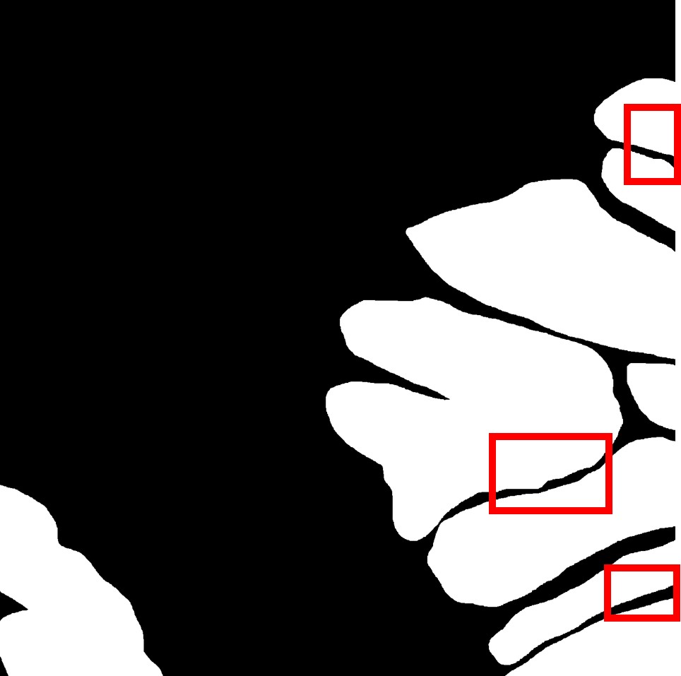
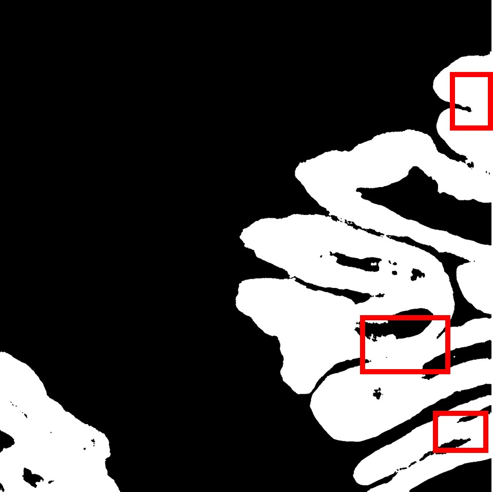
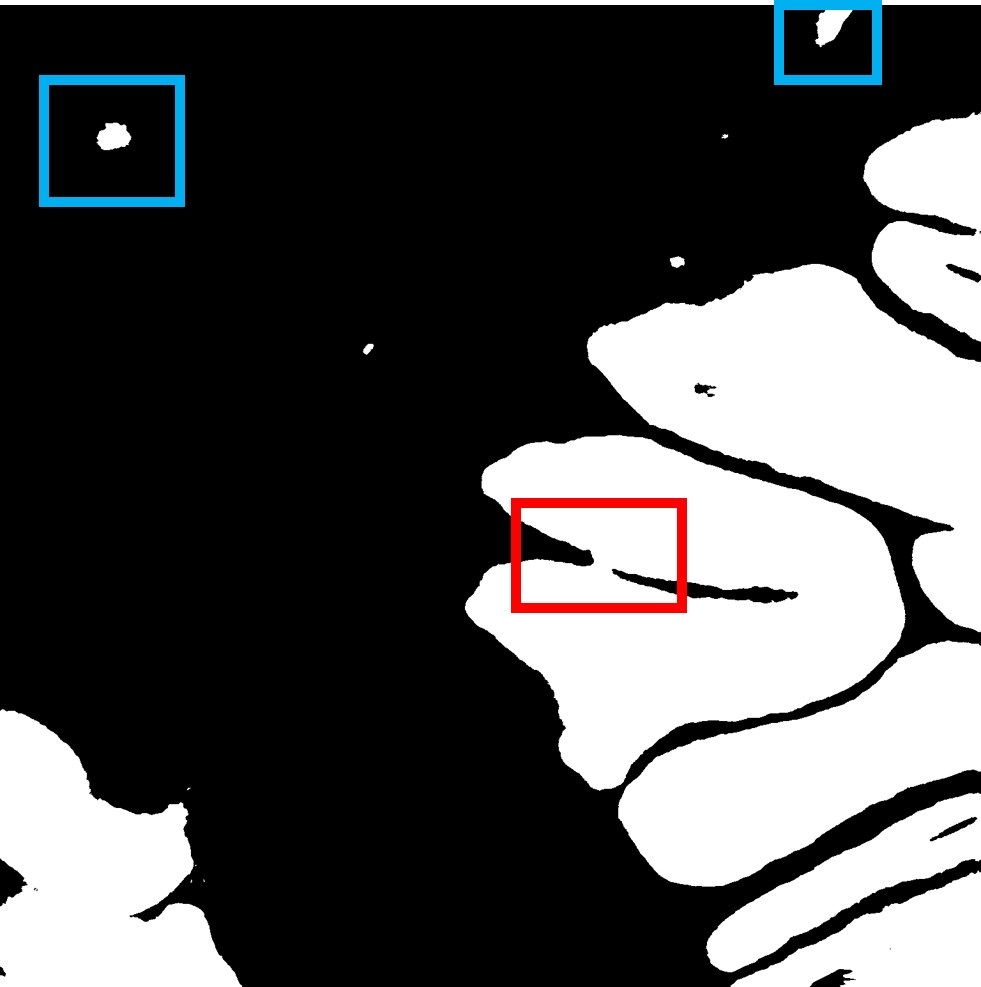
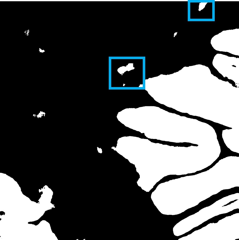
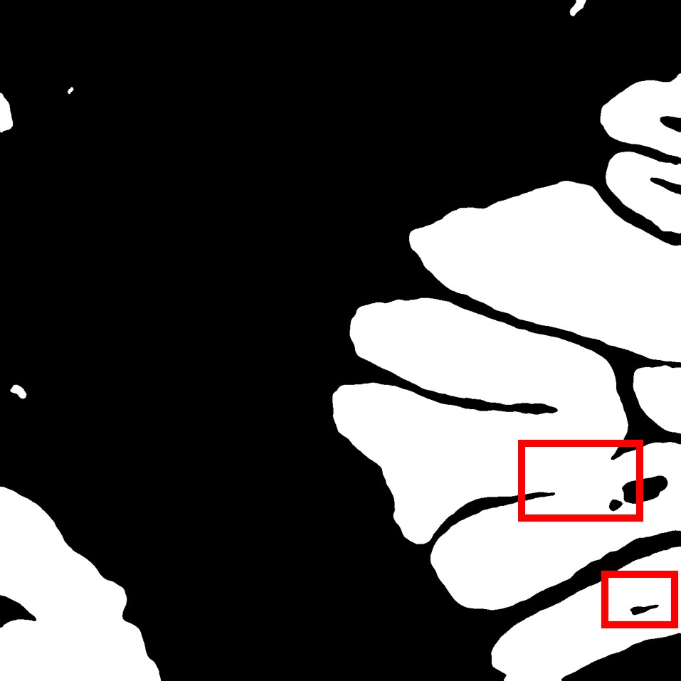
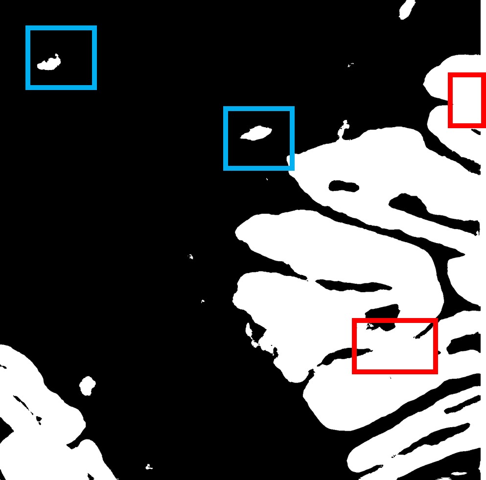
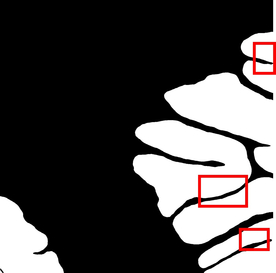
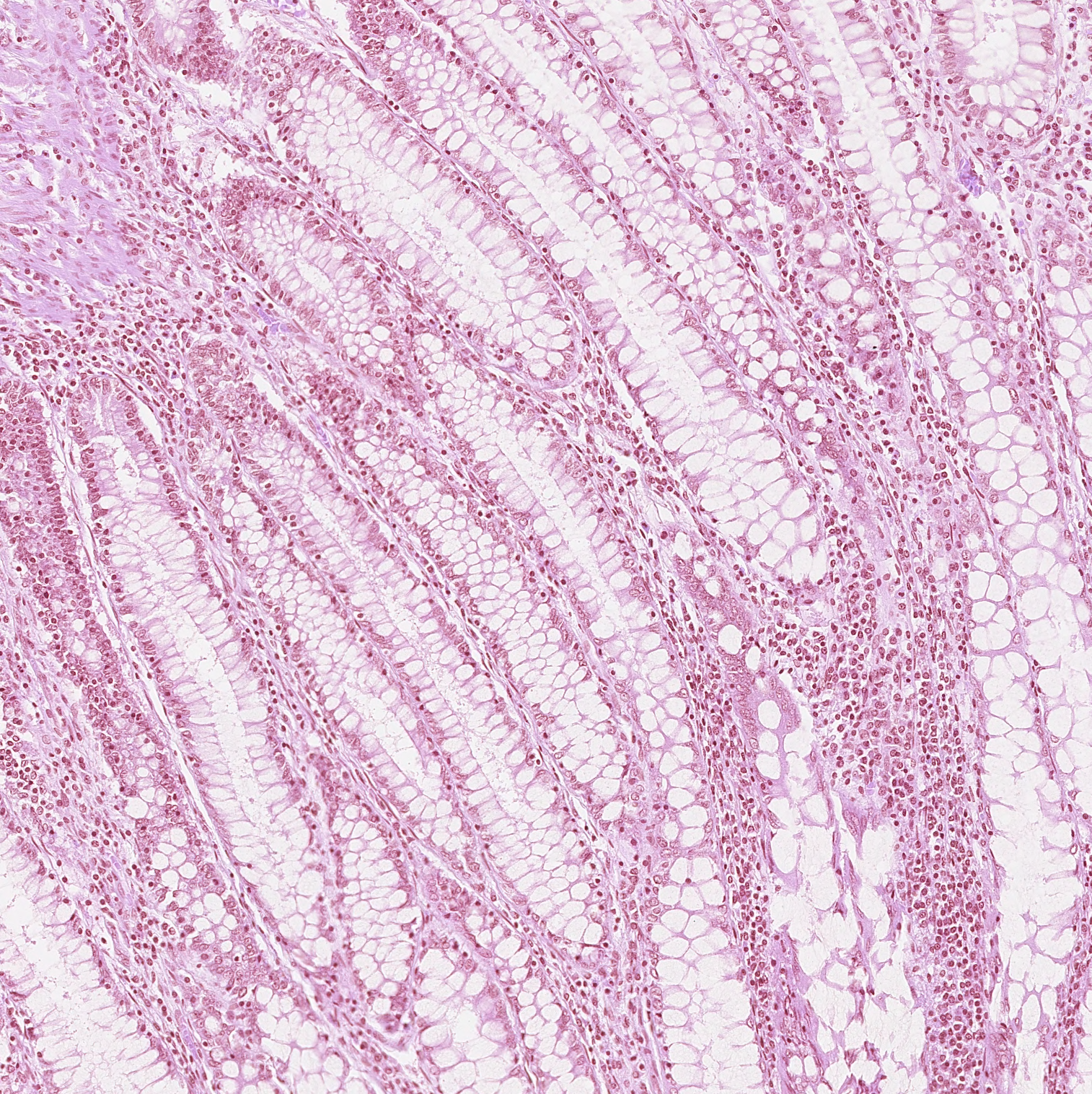
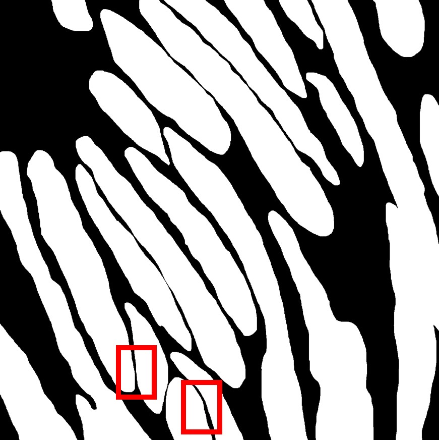
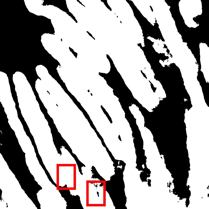
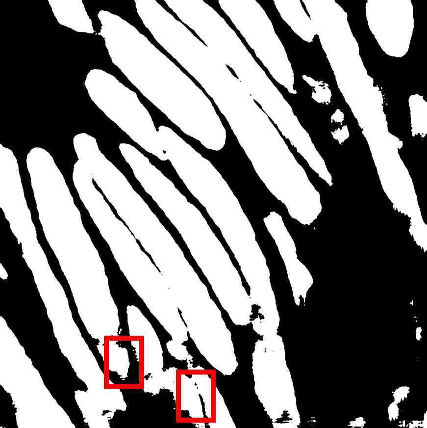
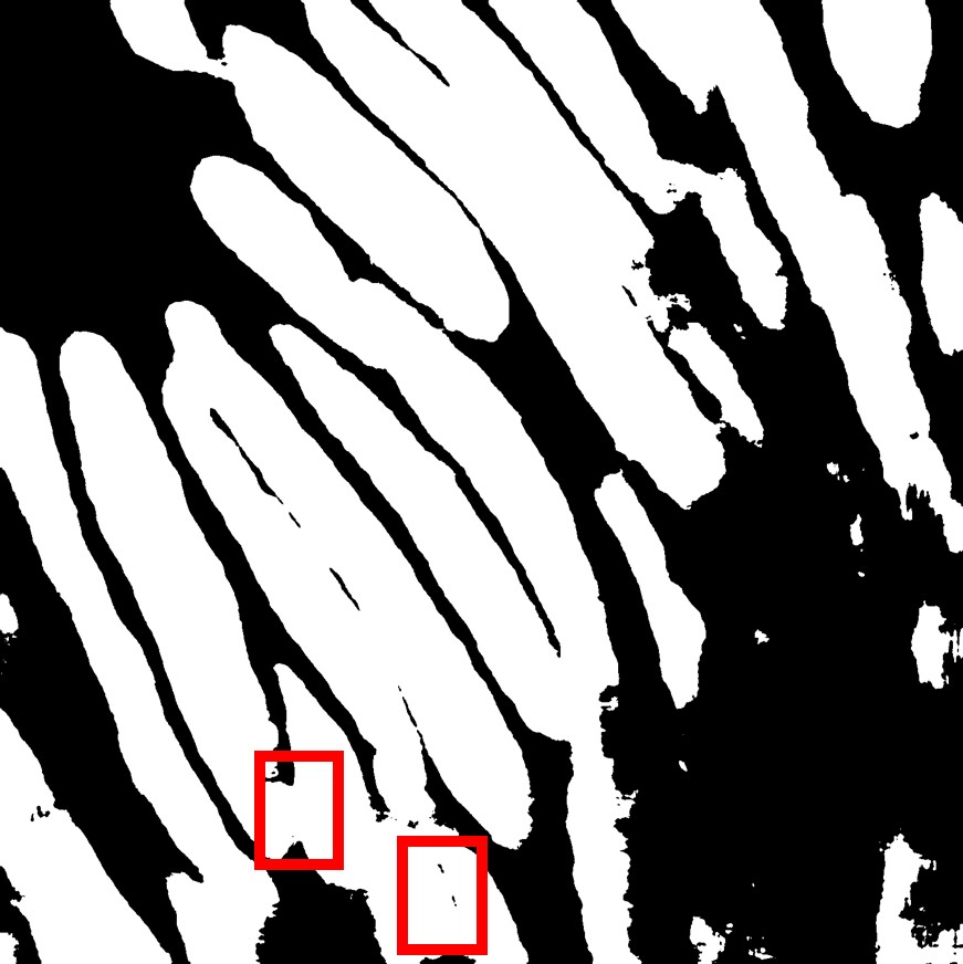
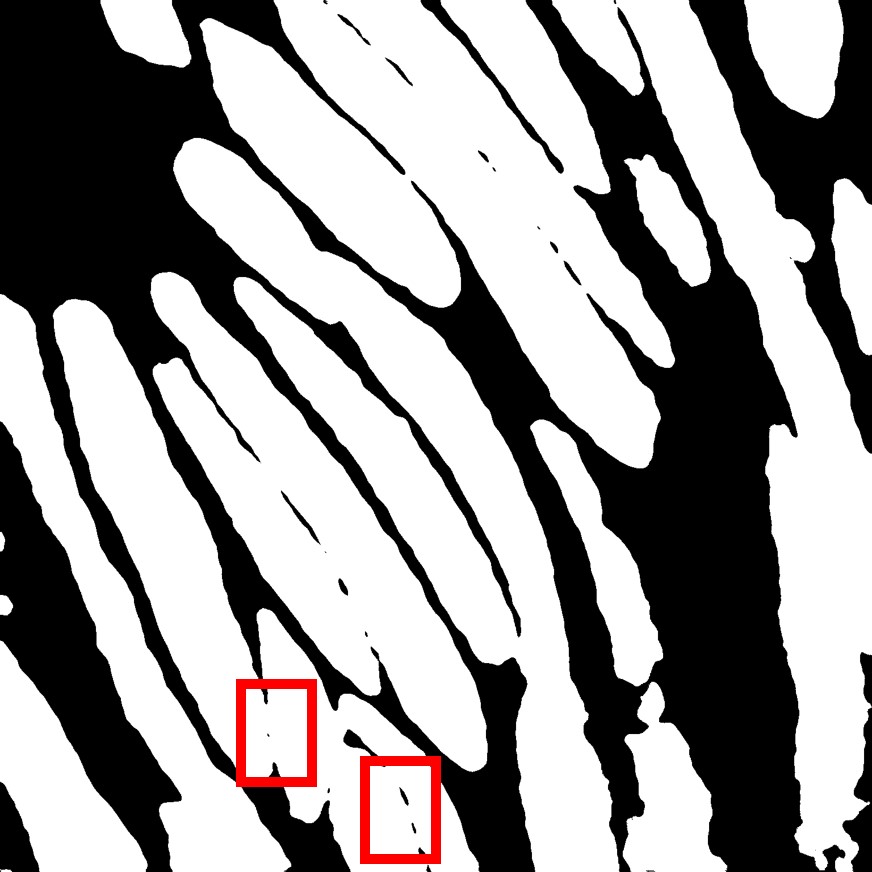
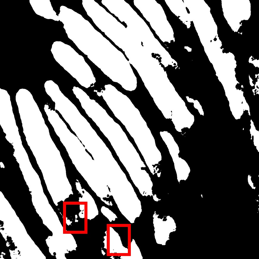
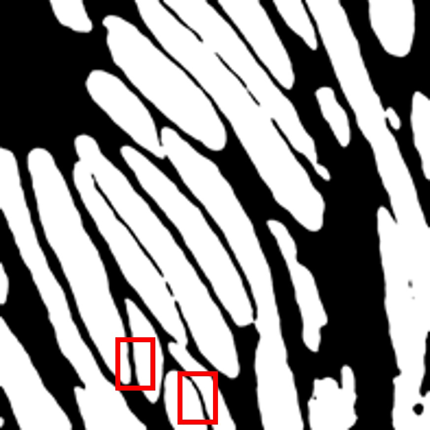
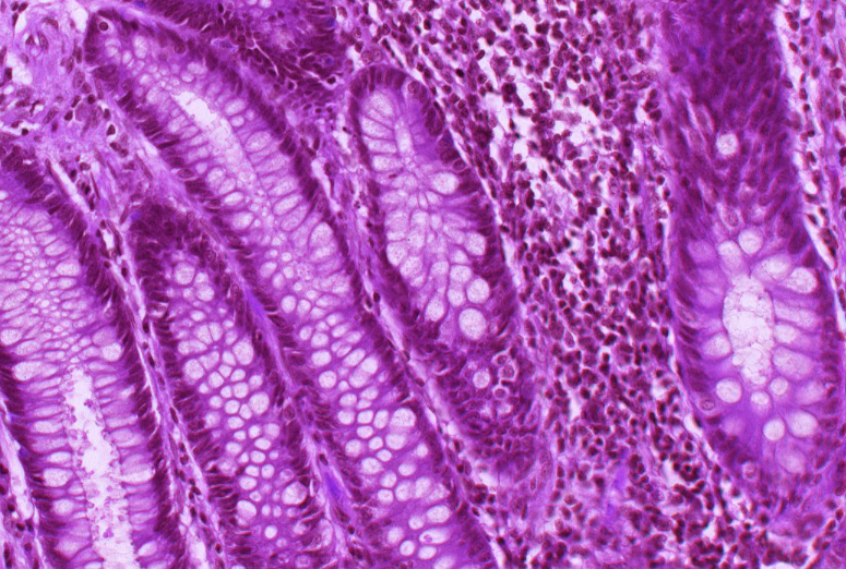
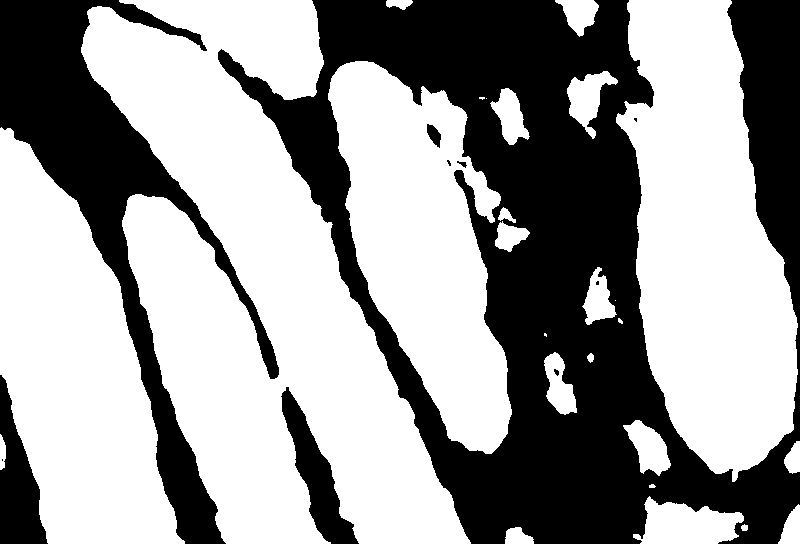
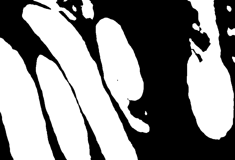
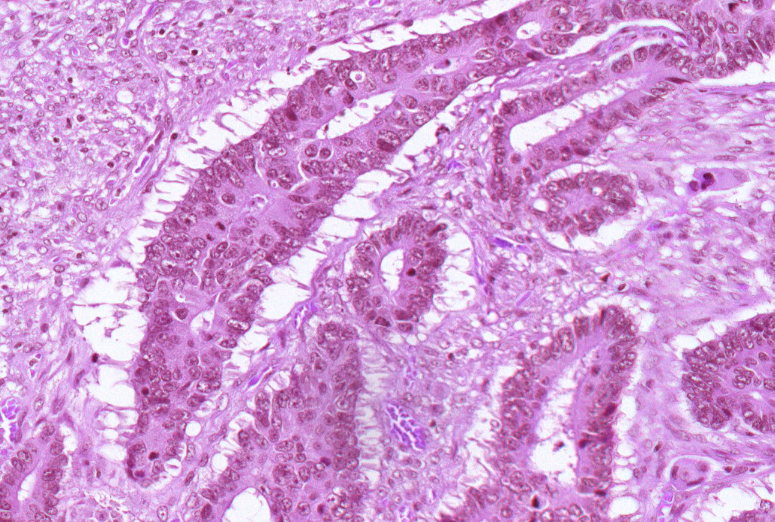
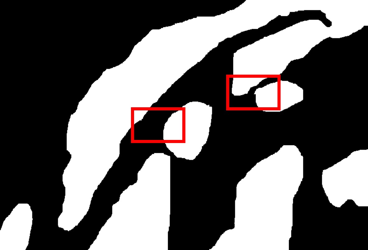
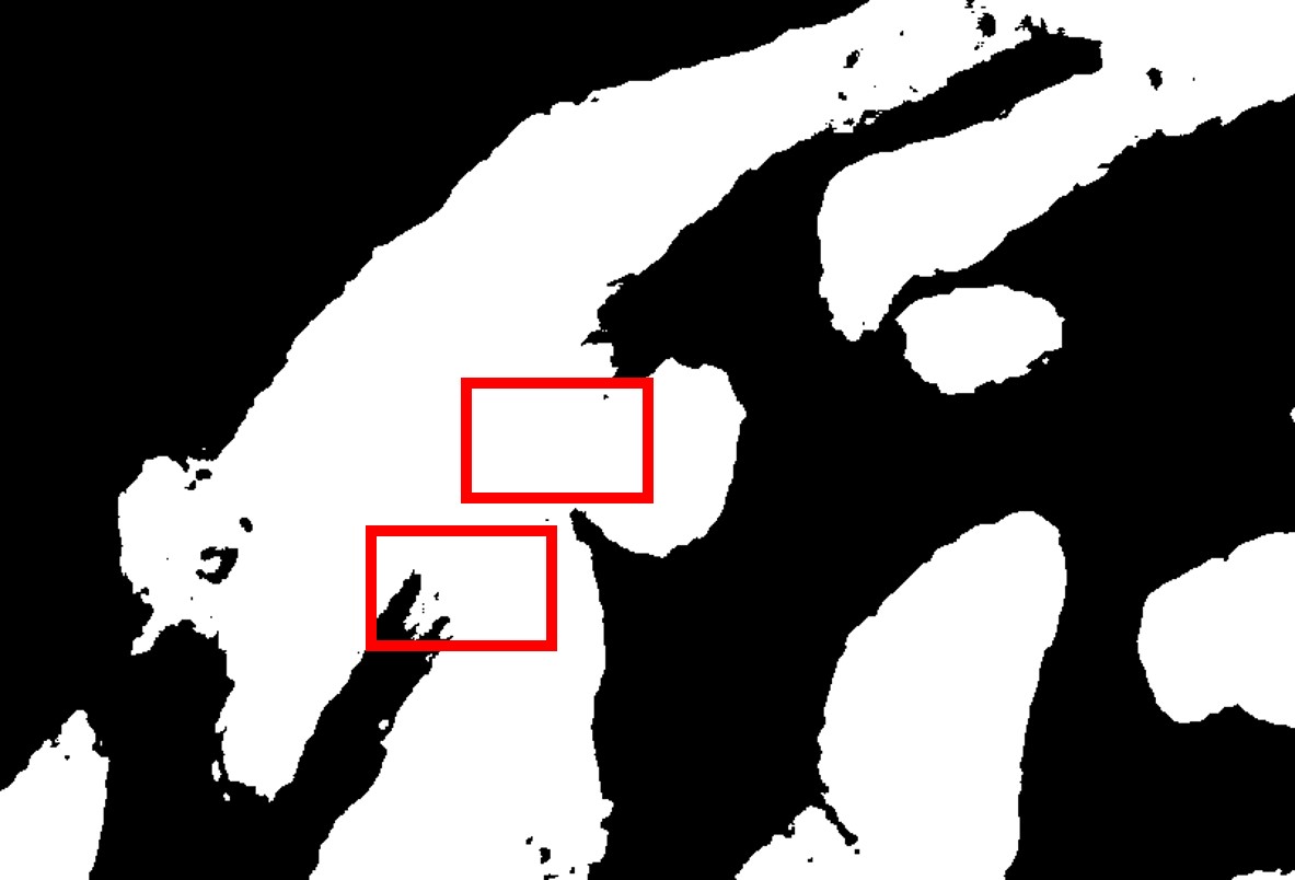
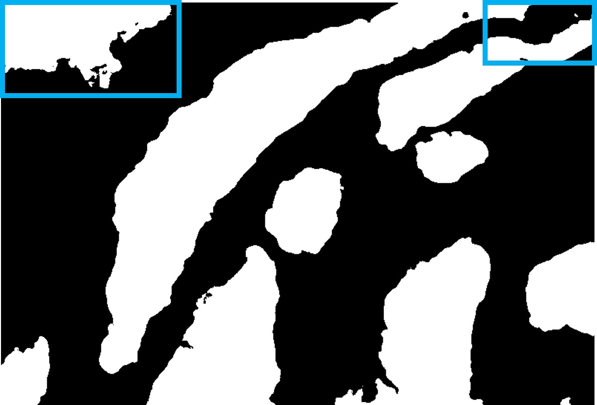
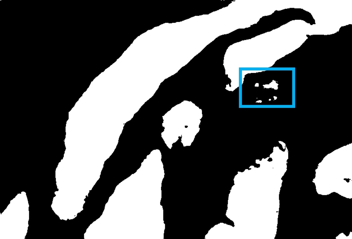
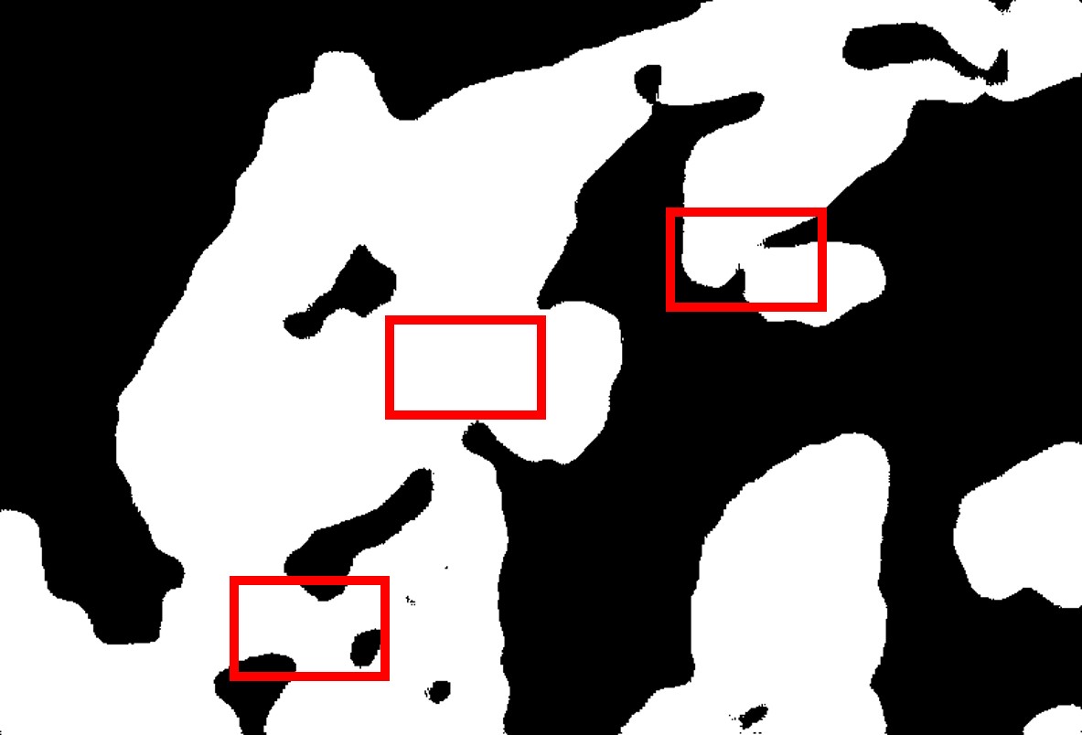
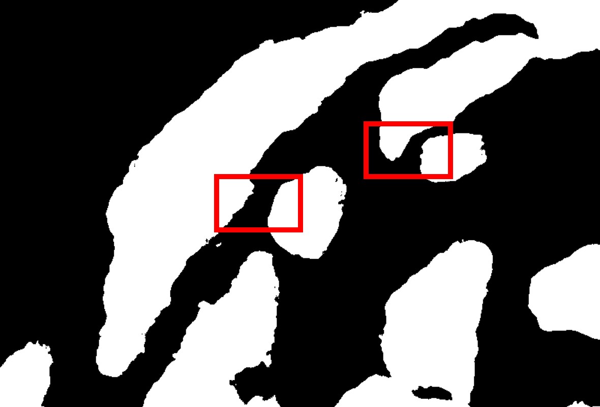
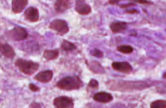
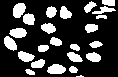
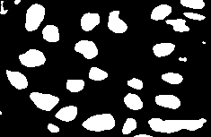
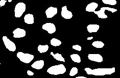
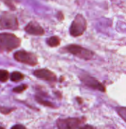
(a) Raw Image

(b) Ground Truth

(c) MT

(d) EM

(e) UA-MT

(f) HCE

(g) URPC

(h) Ours

Figure 7: Additional qualitative results. The red boxes indicate the regions that are prone to topological errors such as incorrect merging or separating adjacent glands; the blue boxes indicate false positive gland predictions or missing glands. Rows 1-2: CRAG. Rows 3-4: GlaS. Rows 5-6: MoNuSeg. Zoom in for better views.

11 Evaluation Metrics

We select three widely used pixel-wise evaluation metrics, Object-level Dice coefficient (Dice_Obj) [57], Intersection over Union (IoU) and Pixel-wise accuracy. Object-level Dice coefficient mainly measures the similarity between two segmented objects, and this is especially useful in pathology imaging, where accurately segmenting individual anatomical structures is crucial. IoU provides a measure of how well the predicted segmentation or detected object aligns with the ground truth. Pixel-wise accuracy evaluates how many pixels in the segmentation maps are correctly classified. The larger these three metrics are, the better the segmentation performance is.

Topology-relevant metrics mainly measure structural accuracy. We also select three topological evaluation metrics, Betti Error [19], Betti Matching Error [47], and Variation of Information (VOI) [36]. For the Betti error, we split the prediction and ground truth into patches in a sliding-window fashion and calculate the average absolute discrepancy between their 0-dimensional Betti number. The size of the window is $256\times 256$. Betti matching error considers the spatial location of the features within their respective images and can be regarded as a variant of Betti error. VOI mainly measures the distance between two clusterings. The smaller these metrics are, the better the segmentation performance is.

+ $\mathcal{L}^{\text{S}}_{\text{topo}}$	+ $\mathcal{L}^{\text{U}}_{\text{topo}}$	Pixel-Wise		Topology-Wise
		Dice_Obj		BE	BME	VOI
✗	✗	0.887		0.230	10.525	0.783
✓	✗	0.891		0.227	11.625	0.743
✗	✓	0.898		0.226	8.575	0.709

Table 5: Ablation study of TopoLoss for both supervised and unsupervised settings.

12 Additional Qualitative Results

Here, we provide more qualitative results in Fig. 7 further to verify the effectiveness and superiority of our proposed method.

13 Ablation Study on Fully-Sup. Topo Loss [19]

To further verify the effectiveness of our proposed topological consistency loss, we conduct an ablation study on fully supervised topological loss [19]. The results are shown in Tab. 5. The third row is our proposed method. We can observe that if we only add topological loss on labeled data, the guidance is insufficient due to the limited amount of annotations. The loss weights are the same for the fully supervised topological loss and topological consistency loss.

References

- Basak and Yin [2023] Hritam Basak and Zhaozheng Yin. Pseudo-label guided contrastive learning for semi-supervised medical image segmentation. In CVPR, 2023.
- Berthelot et al. [2019] David Berthelot, Nicholas Carlini, Ian Goodfellow, Nicolas Papernot, Avital Oliver, and Colin A Raffel. Mixmatch: A holistic approach to semi-supervised learning. In NeurIPS, 2019.
- Cao et al. [2022] Hu Cao, Yueyue Wang, Joy Chen, Dongsheng Jiang, Xiaopeng Zhang, Qi Tian, and Manning Wang. Swin-unet: Unet-like pure transformer for medical image segmentation. In ECCV, 2022.
- Chen et al. [2021] Gaoxiang Chen, Jintao Ru, Yilin Zhou, Islem Rekik, Zhifang Pan, Xiaoming Liu, Yezhi Lin, Beichen Lu, and Jialin Shi. Mtans: Multi-scale mean teacher combined adversarial network with shape-aware embedding for semi-supervised brain lesion segmentation. NeuroImage, 2021.
- Chen et al. [2018] Liang-Chieh Chen, Yukun Zhu, George Papandreou, Florian Schroff, and Hartwig Adam. Encoder-decoder with atrous separable convolution for semantic image segmentation. In ECCV, 2018.
- Clough et al. [2020] James R Clough, Nicholas Byrne, Ilkay Oksuz, Veronika A Zimmer, Julia A Schnabel, and Andrew P King. A topological loss function for deep-learning based image segmentation using persistent homology. TPAMI, 2020.
- Cohen-Steiner et al. [2005] David Cohen-Steiner, Herbert Edelsbrunner, and John Harer. Stability of persistence diagrams. In Proceedings of the twenty-first annual symposium on Computational geometry, 2005.
- Cohen-Steiner et al. [2010] David Cohen-Steiner, Herbert Edelsbrunner, John Harer, and Yuriy Mileyko. Lipschitz functions have l p-stable persistence. Foundations of Computational Mathematics, 2010.
- Edelsbrunner et al. [2002] Edelsbrunner, Letscher, and Zomorodian. Topological persistence and simplification. Discrete & Computational Geometry, 2002.
- Edelsbrunner and Harer [2022] Herbert Edelsbrunner and John L Harer. Computational topology: an introduction. American Mathematical Society, 2022.
- Fang and Li [2020] Kang Fang and Wu-Jun Li. Dmnet: difference minimization network for semi-supervised segmentation in medical images. In MICCAI, 2020.
- Fleming et al. [2012] Matthew Fleming, Sreelakshmi Ravula, Sergei F Tatishchev, and Hanlin L Wang. Colorectal carcinoma: Pathologic aspects. Journal of Gastrointestinal Oncology, 2012.
- Graham et al. [2019] Simon Graham, Hao Chen, Jevgenij Gamper, Qi Dou, Pheng-Ann Heng, David Snead, Yee Wah Tsang, and Nasir Rajpoot. Mild-net: Minimal information loss dilated network for gland instance segmentation in colon histology images. MedIA, 2019.
- Grandvalet and Bengio [2004] Yves Grandvalet and Yoshua Bengio. Semi-supervised learning by entropy minimization. In NeurIPS, 2004.
- Gupta et al. [2022] Saumya Gupta, Xiaoling Hu, James Kaan, Michael Jin, Mutshipay Mpoy, Katherine Chung, Gagandeep Singh, Mary Saltz, Tahsin Kurc, Joel Saltz, et al. Learning topological interactions for multi-class medical image segmentation. In ECCV, 2022.
- Gupta et al. [2023] Saumya Gupta, Yikai Zhang, Xiaoling Hu, Prateek Prasanna, and Chao Chen. Topology-aware uncertainty for image segmentation. In NeurIPS, 2023.
- He et al. [2023] Hongliang He, Jun Wang, Pengxu Wei, Fan Xu, Xiangyang Ji, Chang Liu, and Jie Chen. Toposeg: Topology-aware nuclear instance segmentation. In ICCV, 2023.
- Hu [2022] Xiaoling Hu. Structure-aware image segmentation with homotopy warping. In NeurIPS, 2022.
- Hu et al. [2019] Xiaoling Hu, Fuxin Li, Dimitris Samaras, and Chao Chen. Topology-preserving deep image segmentation. In NeurIPS, 2019.
- Hu et al. [2021] Xiaoling Hu, Yusu Wang, Li Fuxin, Dimitris Samaras, and Chao Chen. Topology-aware segmentation using discrete morse theory. In ICLR, 2021.
- Hu et al. [2023] Xiaoling Hu, Dimitris Samaras, and Chao Chen. Learning probabilistic topological representations using discrete morse theory. In ICLR, 2023.
- Huang et al. [2022] Wei Huang, Chang Chen, Zhiwei Xiong, Yueyi Zhang, Xuejin Chen, Xiaoyan Sun, and Feng Wu. Semi-supervised neuron segmentation via reinforced consistency learning. TMI, 2022.
- Isensee et al. [2021] Fabian Isensee, Paul F Jaeger, Simon AA Kohl, Jens Petersen, and Klaus H Maier-Hein. nnu-net: a self-configuring method for deep learning-based biomedical image segmentation. Nature Methods, 2021.
- Jeong et al. [2019] Jisoo Jeong, Seungeui Lee, Jeesoo Kim, and Nojun Kwak. Consistency-based semi-supervised learning for object detection. In NeurIPS, 2019.
- Jiao et al. [2022] Rushi Jiao, Yichi Zhang, Le Ding, Rong Cai, and Jicong Zhang. Learning with limited annotations: a survey on deep semi-supervised learning for medical image segmentation. arXiv preprint arXiv:2207.14191, 2022.
- Jin et al. [2022a] Qiangguo Jin, Hui Cui, Changming Sun, Jiangbin Zheng, Leyi Wei, Zhenyu Fang, Zhaopeng Meng, and Ran Su. Semi-supervised histological image segmentation via hierarchical consistency enforcement. In MICCAI, 2022a.
- Jin et al. [2022b] Ying Jin, Jiaqi Wang, and Dahua Lin. Semi-supervised semantic segmentation via gentle teaching assistant. In NeurIPS, 2022b.
- Karasaki et al. [2023] Takahiro Karasaki, David A Moore, Selvaraju Veeriah, Cristina Naceur-Lombardelli, Antonia Toncheva, Neil Magno, Sophia Ward, Maise Al Bakir, Thomas BK Watkins, Kristiana Grigoriadis, et al. Evolutionary characterization of lung adenocarcinoma morphology in tracerx. Nature Medicine, 2023.
- Kerber et al. [2016] Michael Kerber, Dmitriy Morozov, and Arnur Nigmetov. Geometry helps to compare persistence diagrams. In 2016 Proceedings of the Eighteenth Workshop on Algorithm Engineering and Experiments (ALENEX), pages 103–112. SIAM, 2016.
- Kumar et al. [2019] Neeraj Kumar, Ruchika Verma, Deepak Anand, Yanning Zhou, Omer Fahri Onder, Efstratios Tsougenis, Hao Chen, Pheng-Ann Heng, Jiahui Li, Zhiqiang Hu, et al. A multi-organ nucleus segmentation challenge. TMI, 2019.
- Lacombe et al. [2018] Théo Lacombe, Marco Cuturi, and Steve Oudot. Large scale computation of means and clusters for persistence diagrams using optimal transport. NeurIPS, 2018.
- Li et al. [2023] Chen Li, Xiaoling Hu, Shahira Abousamra, and Chao Chen. Calibrating uncertainty for semi-supervised crowd counting. In ICCV, 2023.
- Li et al. [2020] Xiaomeng Li, Lequan Yu, Hao Chen, Chi-Wing Fu, Lei Xing, and Pheng-Ann Heng. Transformation-consistent self-ensembling model for semisupervised medical image segmentation. TNNLS, 2020.
- Li et al. [2021] Yanwen Li, Luyang Luo, Huangjing Lin, Hao Chen, and Pheng-Ann Heng. Dual-consistency semi-supervised learning with uncertainty quantification for covid-19 lesion segmentation from ct images. In MICCAI, 2021.
- Luo et al. [2022] Xiangde Luo, Guotai Wang, Wenjun Liao, Jieneng Chen, Tao Song, Yinan Chen, Shichuan Zhang, Dimitris N Metaxas, and Shaoting Zhang. Semi-supervised medical image segmentation via uncertainty rectified pyramid consistency. MedIA, 2022.
- Meilă [2003] Marina Meilă. Comparing clusterings by the variation of information. In Learning Theory and Kernel Machines: 16th Annual Conference on Learning Theory and 7th Kernel Workshop, COLT/Kernel 2003, 2003.
- Montironi et al. [2005] Rodolfo Montironi, Roberta Mazzuccheli, Marina Scarpelli, Antonio Lopez-Beltran, Giovanni Fellegara, and Ferran Algaba. Gleason grading of prostate cancer in needle biopsies or radical prostatectomy specimens: contemporary approach, current clinical significance and sources of pathology discrepancies. BJU International, 2005.
- Munkres [1984] James R Munkres. Elements of algebraic topology, 1984.
- Oner et al. [2023] Doruk Oner, Adélie Garin, Mateusz Koziński, Kathryn Hess, and Pascal Fua. Persistent homology with improved locality information for more effective delineation. TPAMI, 2023.
- Ouali et al. [2020] Yassine Ouali, Céline Hudelot, and Myriam Tami. Semi-supervised semantic segmentation with cross-consistency training. In CVPR, 2020.
- Ronneberger et al. [2015] Olaf Ronneberger, Philipp Fischer, and Thomas Brox. U-net: Convolutional networks for biomedical image segmentation. In MICCAI, 2015.
- Seibold et al. [2022] Constantin Marc Seibold, Simon Reiß, Jens Kleesiek, and Rainer Stiefelhagen. Reference-guided pseudo-label generation for medical semantic segmentation. In AAAI, 2022.
- Shi et al. [2021] Yinghuan Shi, Jian Zhang, Tong Ling, Jiwen Lu, Yefeng Zheng, Qian Yu, Lei Qi, and Yang Gao. Inconsistency-aware uncertainty estimation for semi-supervised medical image segmentation. TMI, 2021.
- Shit et al. [2021] Suprosanna Shit, Johannes C Paetzold, Anjany Sekuboyina, Ivan Ezhov, Alexander Unger, Andrey Zhylka, Josien PW Pluim, Ulrich Bauer, and Bjoern H Menze. cldice-a novel topology-preserving loss function for tubular structure segmentation. In CVPR, 2021.
- Sirinukunwattana et al. [2017] Korsuk Sirinukunwattana, Josien PW Pluim, Hao Chen, Xiaojuan Qi, Pheng-Ann Heng, Yun Bo Guo, Li Yang Wang, Bogdan J Matuszewski, Elia Bruni, Urko Sanchez, et al. Gland segmentation in colon histology images: The glas challenge contest. MedIA, 2017.
- Sohn et al. [2020] Kihyuk Sohn, David Berthelot, Nicholas Carlini, Zizhao Zhang, Han Zhang, Colin A Raffel, Ekin Dogus Cubuk, Alexey Kurakin, and Chun-Liang Li. Fixmatch: Simplifying semi-supervised learning with consistency and confidence. In NeurIPS, 2020.
- Stucki et al. [2023] Nico Stucki, Johannes C Paetzold, Suprosanna Shit, Bjoern Menze, and Ulrich Bauer. Topologically faithful image segmentation via induced matching of persistence barcodes. In ICML, 2023.
- Sudre et al. [2017] Carole H Sudre, Wenqi Li, Tom Vercauteren, Sebastien Ourselin, and M Jorge Cardoso. Generalised dice overlap as a deep learning loss function for highly unbalanced segmentations. In Deep Learning in Medical Image Analysis and Multimodal Learning for Clinical Decision Support: Third International Workshop, DLMIA 2017, and 7th International Workshop, ML-CDS 2017, Held in Conjunction with MICCAI 2017, 2017.
- Tarvainen and Valpola [2017] Antti Tarvainen and Harri Valpola. Mean teachers are better role models: Weight-averaged consistency targets improve semi-supervised deep learning results. In NeurIPS, 2017.
- Thompson et al. [2022] Bethany H Thompson, Gaetano Di Caterina, and Jeremy P Voisey. Pseudo-label refinement using superpixels for semi-supervised brain tumour segmentation. In ISBI, 2022.
- Vu et al. [2019] Tuan-Hung Vu, Himalaya Jain, Maxime Bucher, Matthieu Cord, and Patrick Pérez. Advent: Adversarial entropy minimization for domain adaptation in semantic segmentation. In CVPR, 2019.
- Wang et al. [2022a] Haonan Wang, Peng Cao, Jiaqi Wang, and Osmar R Zaiane. Uctransnet: rethinking the skip connections in u-net from a channel-wise perspective with transformer. In AAAI, 2022a.
- Wang et al. [2022b] Haotian Wang, Min Xian, and Aleksandar Vakanski. Ta-net: Topology-aware network for gland segmentation. In WACV, 2022b.
- Wang et al. [2022c] Xiaoyan Wang, Yiwen Yuan, Dongyan Guo, Xiaojie Huang, Ying Cui, Ming Xia, Zhenhua Wang, Cong Bai, and Shengyong Chen. Ssa-net: Spatial self-attention network for covid-19 pneumonia infection segmentation with semi-supervised few-shot learning. MedIA, 2022c.
- Wu et al. [2022a] Huisi Wu, Zhaoze Wang, Youyi Song, Lin Yang, and Jing Qin. Cross-patch dense contrastive learning for semi-supervised segmentation of cellular nuclei in histopathologic images. In CVPR, 2022a.
- Wu et al. [2022b] Yicheng Wu, Zongyuan Ge, Donghao Zhang, Minfeng Xu, Lei Zhang, Yong Xia, and Jianfei Cai. Mutual consistency learning for semi-supervised medical image segmentation. MedIA, 2022b.
- Xie et al. [2019] Yutong Xie, Hao Lu, Jianpeng Zhang, Chunhua Shen, and Yong Xia. Deep segmentation-emendation model for gland instance segmentation. In MICCAI, 2019.
- Yao et al. [2022] Huifeng Yao, Xiaowei Hu, and Xiaomeng Li. Enhancing pseudo label quality for semi-supervised domain-generalized medical image segmentation. In AAAI, 2022.
- You et al. [2022] Chenyu You, Yuan Zhou, Ruihan Zhao, Lawrence Staib, and James S Duncan. Simcvd: Simple contrastive voxel-wise representation distillation for semi-supervised medical image segmentation. TMI, 2022.
- You et al. [2023] Chenyu You, Weicheng Dai, Yifei Min, Fenglin Liu, Xiaoran Zhang, Chen Feng, David A Clifton, S Kevin Zhou, Lawrence Hamilton Staib, and James S Duncan. Rethinking semi-supervised medical image segmentation: A variance-reduction perspective. In NeurIPS, 2023.
- Yu et al. [2019] Lequan Yu, Shujun Wang, Xiaomeng Li, Chi-Wing Fu, and Pheng-Ann Heng. Uncertainty-aware self-ensembling model for semi-supervised 3d left atrium segmentation. In MICCAI, 2019.
- Zhang et al. [2022a] Wenqiao Zhang, Lei Zhu, James Hallinan, Shengyu Zhang, Andrew Makmur, Qingpeng Cai, and Beng Chin Ooi. Boostmis: Boosting medical image semi-supervised learning with adaptive pseudo labeling and informative active annotation. In CVPR, 2022a.
- Zhang et al. [2022b] Zhenxi Zhang, Chunna Tian, Harrison X Bai, Zhicheng Jiao, and Xilan Tian. Discriminative error prediction network for semi-supervised colon gland segmentation. MedIA, 2022b.
- Zhao et al. [2017] Hengshuang Zhao, Jianping Shi, Xiaojuan Qi, Xiaogang Wang, and Jiaya Jia. Pyramid scene parsing network. In CVPR, 2017.
- Zhou et al. [2023] Yanfeng Zhou, Jiaxing Huang, Chenlong Wang, Le Song, and Ge Yang. Xnet: Wavelet-based low and high frequency fusion networks for fully-and semi-supervised semantic segmentation of biomedical images. In ICCV, 2023.
- Zhou et al. [2018] Zongwei Zhou, Md Mahfuzur Rahman Siddiquee, Nima Tajbakhsh, and Jianming Liang. Unet++: A nested u-net architecture for medical image segmentation. In Deep Learning in Medical Image Analysis and Multimodal Learning for Clinical Decision Support: 4th International Workshop, DLMIA 2018, and 8th International Workshop, ML-CDS 2018, Held in Conjunction with MICCAI 2018, 2018.