Learning Markovian Dynamics with Spectral Maps

Abstract

The long-time behavior of many complex molecular systems is often governed by slow relaxation dynamics that can be described by a few reaction coordinates referred to as collective variables (CVs). However, identifying CVs hidden in a high-dimensional configuration space poses a fundamental challenge in chemical physics. To address this problem, we expand on a recently introduced deep-learning technique called spectral map [Rydzewski, J. Phys. Chem. Lett. 2023, 14, 22, 5216–5220]. Spectral map learns CVs by maximizing a spectral gap between slow and fast eigenvalues of a Markov transition matrix describing anisotropic diffusion. An introduced modification in the learning algorithm allows spectral map to represent multiscale free-energy landscapes. Through a Markov state model analysis, we validate that spectral map learns slow CVs related to the dominant relaxation timescales and discerns between long-lived metastable states.

I Introduction

Understanding the long timescale dynamics of complex molecular systems constitutes a fundamental problem in chemical physics [1]. This dynamics is often governed by rare transitions between multiple long-lived metastable states that involve overcoming energy barriers much higher than the thermal energy ($\gg k_{\mathrm{B}}T$) [2, 3]. Systems exhibiting metastable features, while characterized by many variables and timescales, frequently display slow relaxation dynamics that can be captured by a few reaction coordinates, also called collective variables (CVs), to demarcate between metastable states [4, 5]. The long timescale dynamics is often viewed as effectively Markovian and modeled as diffusion in a free-energy landscape [6, 7]. Under this view, the dynamics is governed mainly by slowly varying variables, while fast variables are treated as uncoupled thermal noise, leading to adiabatic timescale separation.

Relying merely on physical intuition or trial and error to identify slow CVs can be unsystematic and result in highly non-Markovian dynamics with long memory effects, which can hinder the understanding of the underlying physical process [8]. This problem of timescale separation has been addressed in the Mori–Zwanzig projection operator formalism by constructing a generalized Langevin equation that describes the dynamics in a slow subspace. However, as noted by Zwanzig, “no a priori choice is specifically indicated by theory” [9]. Recently, there has been a growing interest in constructing simplified representations of complex systems for atomistic simulations using data-driven techniques [10, 11, 12, 13]. One class of such methods tackles disentangling slow and fast kinetics, which is particularly useful in metastable systems that involve multiple temporal scales [14, 15, 16, 17, 18, 19, 20, 21, 22, 23, 24, 25, 26, 27, 28].

In this Communication, we present spectral map [28], an unsupervised machine-learning technique inspired by diffusion map [29, 30, 31] and parametric dimensionality reduction [32, 33, 34, 35, 36]. Spectral map learns CVs by maximizing a spectral gap between slow and fast eigenvalues of a Markov transition matrix, preventing memory effects, which leads to effective slow dynamics relevant to the physical system. We improve the training algorithm by introducing an adaptive algorithm that allows spectral map to represent accurately the multiscale free-energy landscape of long-lived metastable states. Finally, through a standard Markov state model analysis, we validate that CVs constructed by spectral map encode dominant slow relaxation timescales.

II Collective Variables

Consider a high-dimensional system described by $n$ configuration variables $\mathbf{x}=(x_{1},\dots,x_{n})$ whose dynamics at temperature $T$ is driven according to a potential energy function $U(\mathbf{x})$, and sampled generally from an unknown equilibrium distribution. However, if we represent the system using the microscopic coordinates, its dynamics proceeds according to a canonical equilibrium distribution given by the Boltzmann density $p(\mathbf{x})\propto\operatorname{e}^{-\beta U(\mathbf{x})}$, where $\beta=(1/k_{\mathrm{B}}T)$ is the inverse temperature, $k_{\mathrm{B}}$ is the Boltzmann constant and $Z=\int\operatorname{d\mathbf{x}}\operatorname{e}^{-\beta U(\mathbf{x})}$ is the partition function of the system.

We simplify the high-dimensional configuration space by mapping it into a reduced space $\mathbf{z}=\left(z_{1},\dots,z_{d}\right)$ given by a set of $d$ functions of the configuration variables, commonly referred to as CVs, where $d\ll n$. We encapsulate these functions in a target mapping [35, 36, 12]:

$$\mathbf{z}=\xi_{w}(\mathbf{x})\equiv\big{\{}\xi_{k}(\mathbf{x},w)\big{\}}_{k=1}^{d},$$ (1)

where $w$ are learnable parameters ensuring that the target mapping describes slow dynamics and minimizes memory effects. By sampling the system in the CV space, its dynamics follows a marginal equilibrium density $p(\mathbf{z})\propto\operatorname{e}^{-\beta F(\mathbf{z})}$, where $F(\mathbf{z})$ is a free-energy landscape:

$$F(\mathbf{z})=-\frac{1}{\beta}\log\int\operatorname{d\mathbf{x}}\,\delta\left(\mathbf{z}-\xi_{\theta}(\mathbf{x})\right)\operatorname{e}^{-\beta U(\mathbf{x})}.$$ (2)

To learn the target mapping, we gather as input a tensor of $N$ high-dimensional configuration samples from a molecular simulation:

$$X=(\mathbf{x}_{1},\dots,\mathbf{x}_{N})^{\top}\in\mathbb{R}^{N\times n}.$$ (3)

As $N$ is usually large, we need to learn an “optimal” parameterization using a stochastic procedure by representing the target mapping as a neural network with a score function specifically devised to ensure that the learned CVs are slow and correspond to rare transitions between free-energy basins.

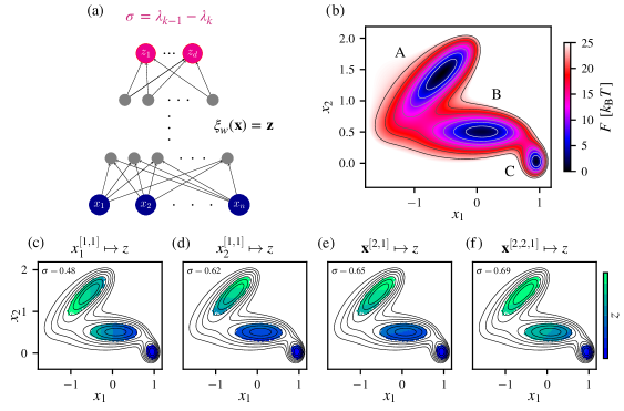
Figure 1: Training the target mapping $\xi_{w}(\mathbf{x})=\mathbf{z}$ on the three-state Müller–Brown potential from Ref. 37. (a) Schematic outline of a neural network used to model the target mapping. The reduction from high-dimensional variables $\mathbf{x}$ is performed to obtain low-dimensional slow CVs $\mathbf{z}$ by maximizing the spectral gap $\sigma=\lambda_{k-1}-\lambda_{k}$, where $k$ is the number of the metastable states in the CV space, and $\{\lambda_{k}\}$ are eigenvalues from the spectral decomposition of the Markov transition matrix $M$ [Eq. 7]. (b) Free-energy landscape of a particle moving in the two-dimensional space $\mathbf{x}=(x_{1},x_{2})$ with barriers between the states of around 20 $k_{\mathrm{B}}T$ and a kinetic bootleneck between states B and C. (c-f) Examples of training the target mappings employing different network architectures, e.g., $\mathbf{x}^{[a,b]}\mapsto z$ denotes mapping the $\mathbf{x}$ variable through a network consisting of $[a,b]$ layers to the $z$ CV. Spectral gap values $\sigma$ are given in the top-left corners. The following variables are used as CVs: (c) the $x_{1}$ variable, (d) the $x_{2}$ variable, (e) a linear combination of $x_{1}$ and $x_{2}$, (f) a nonlinear combination of $x_{1}$ and $x_{2}$. For additional details and results, see the Supplementary Material.

III Spectral Map

To estimate the timescale separation between effective timescales characteristic of the system, we can model its effective reduced dynamics as a Markov chain using kernel functions. Let us start by encoding a notion of local geometry into the representation of CVs. To achieve this, we introduce an adaptive Gaussian kernel:

$$G(\mathbf{z}_{k},\mathbf{z}_{l})=\exp\left(-\frac{1}{\varepsilon}{\lVert\mathbf{z}_{k}-\mathbf{z}_{l}\rVert^{2}}\right)$$ (4)

to describe similarity based on pairwise Euclidean distances $\lVert\mathbf{z}_{k}-\mathbf{z}_{l}\rVert$ between CV samples. The Gaussian kernel exhibits a notion of locality by defining a neighborhood around each sample of radius $\varepsilon$ [38].

Free-energy landscapes are often spacially heterogeneous, even for simple systems. Thus, the multimodal characteristics of metastable states requires estimating the scale factor $\varepsilon$ adaptively by maintaining a balance between local and global scales. Therefore, to improve the ability of spectral map to adjust to metastable states, we calculate sample-dependent scale factors as:

$$\varepsilon_{kl}=\lVert\mathbf{z}_{k}-\eta_{i}(\mathbf{z}_{k})\rVert\cdot\lVert\mathbf{z}_{l}-\eta_{i}(\mathbf{z}_{l})\rVert,$$ (5)

where $\eta_{i}(\mathbf{z})$ returns the $i$th neighbor of $\mathbf{z}$. In practice, this neighbor is found as $i=rN$, where the parameter $r$ defines the neighborhood size. For small values of $r$, the Gaussian kernel describes a local neighborhood of each sample, but for larger values, it takes into account more global information.

As the marginal equilibrium density in the CV space is unknown, we need a density-preserving kernel for data sampled from any underlying probability distribution. We employ an anisotropic diffusion kernel as introduced in diffusion map [29]:

$$K(\mathbf{z}_{k},\mathbf{z}_{l})=\frac{G(\mathbf{z}_{k},\mathbf{z}_{l})}{\sqrt{\varrho(\mathbf{z}_{k})\varrho(\mathbf{z}_{l})}},$$ (6)

where $\varrho(\mathbf{z}_{k})=\sum_{l}g(\mathbf{z}_{k},\mathbf{z}_{l})$ is a kernel density estimate. As uniform sampling density is rarely observed for dynamical systems with complex free-energy landscapes, the anisotropic diffusion kernel can account on the differences in the CV distribution.

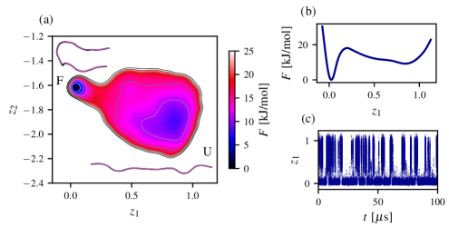
Figure 2: Learning CVs from the reversible folding of CLN025 in solvent sampled through a 100-$\mu$ molecular dynamics simulation. The dataset is obtained from Ref. 39. (a) Spectral map and the related free-energy landscape of CLN025 showing two distinct free-energy basins: the main and well-defined folded (F) and more loosely defined unfolded (U) metastable states, separated by an energy barrier of around 20 kJ/mol. Representative conformations from the metastable states are shown. (b) Free-energy profile shown as a function of the $z_{1}$ CV. (c) Time-series for the $z_{1}$ CV showing transitions between the states.

A Markov transition matrix constructed from Eq. 6 allows to model the dynamics by anisotropic diffusion of a Fokker–Planck equation and, thus, to approximate the long-time behavior of the system [29]. We build the Markov by row-normalizing $K$:

$$m_{kl}\sim M(\mathbf{z}_{k},\mathbf{z}_{l})=\frac{K(\mathbf{z}_{k},\mathbf{z}_{l})}{\sum_{n}K(\mathbf{z}_{k},\mathbf{z}_{n})}$$ (7)

which models a discrete Markov chain in the CV space given by $m_{kl}=\mathrm{Pr}\{\mathbf{z}_{\tau+1}=\mathbf{z}_{l}\;|\;\mathbf{z}_{\tau}=\mathbf{z}_{k}\}$ describing a transition probabilitie between CV samples $\mathbf{z}_{k}$ and $\mathbf{z}_{l}$ in an auxilary (non-physical) time step $\tau$. Next, we calculate a spectral decomposition of the Markov transition matrix defined in the CV space:

$$M\Psi_{k}=\lambda_{k}\Psi_{k},$$ (8)

where $\Psi_{k}$ and $\lambda_{k}$ are the $k$-th right eigenfunctions and eigenvalues of $M$, respectively. The real-valued eigenvalues of $M$ are (sorted in non-ascending order):

$$\lambda_{0}=1>\lambda_{1}\geq\dots\lambda_{d}\dots\geq\lambda_{N}.$$ (9)

Systems exhibiting metastability have a large gap in the spectrum which indicates how many slowly decaying processes are hidden in the dynamics ($d\ll N$). There is only one eigenvalue $\lambda_{0}=1$ that has the greatest value and it corresponds to the equilibrium distribution of $M$ given by the eigenfunction $\Psi_{0}$. The slowest effective relaxation timescales in the system are induced by the dominant eigenvalues:

$$t_{k}=-\frac{1}{\log\lambda_{k}},$$ (10)

for $k>0$ and $t_{0}=\infty$. The largest gap between neighboring eigenvalues is called the spectral gap $\sigma$ and it measures the degree of the effective timescale separation between the slow and fast processes:

$$\sigma=\lambda_{k-1}-\lambda_{k},$$ (11)

where $k>0$ indicates the number of metastable states in the CV space [40]. As a large spectral gap, we can take $\sigma$ that induces a free-energy barrier between metastable states that is much larger than the thermal energy $k_{\mathrm{B}}T$. Thus, maximizing the spectral gap at $k$ results in $k$ metastable states, however, only if the maximal spectral gap is large enough to distinguish between $k$ states.

The theory of spectral characterization of metastable states, as extensively explained by Gaveau and Schulman [40], suggests that the degree of degeneracy in the eigenvalue spectrum is closely related to the timescale separation. For instance, if the eigenvalue of the Markov transition matrix is nearly degenerate $k+1$ times, $\lambda_{k}\approx 1$, this indicates that the equilibrium distribution breaks into $k$ metastable states with infrequent transitions between them. The converse is also true: if the equilibrium density breaks into metastable states with a long transit time between them, then there is eigenvalue degeneracy. However, not only the degeneracy of the dominant eigenvalues is needed, but also a significant spectral gap between the neighboring eigenvalues is required to render the reduced dynamics Markovian [18, 28].

IV Applications

IV.1 Müller–Brown Potential

As a simple demonstration, we apply spectral map to a dataset consisting of several trajectories of a particle moving in a modified three-state Müller–Brown potential [Fig. 1(b)]. The standard Müller–Brown potential is modified by adding a kinetic bottleneck between states B and C [37] (see the Supplementary Material). The input variables for the target mappings are the $\mathbf{x}=(x_{1},x_{2})$ coordinates of the particle. We use the Adam optimizer with a learning rate of $10^{-3}$. The dataset consisting of 80 trajectories initiated at random from the three metastable states is split into batches of size 2000. The training is carried through 30 epochs. The dataset is generated by a Langevin integrator as implemented in PLUMED [41, 42], using a temperature of 1, a friction coefficient of 10, and a time step of 0.005. We set the fraction of samples used to estimate a neighbor for calculating sample-dependent scale constants to $r=0.4$ [Eq. 5].

In Fig. 1(c), we can see that if the $x_{1}$ variable is used as a CV, the spectral gap is just around $\sigma=0.48$. Treating the $x_{2}$ as a CV results in an improved spectral gap of 0.62, as $x_{2}$ is slower than $x_{1}$ and better separates the three states [Fig. 1(d)]. Using a linear combination of $x_{1}$ and $x_{2}$, we can slightly increase the separation between the states [Fig. 1(e)]. Adding a layer with the ELU activation function to the target mapping [Fig. 1(f)], we get a separation with the two main states A and B closer together and the state C pushed farther away as particle reaching this state must overcome a kinetic bottleneck, clearly showing a slow CV should account for this transition and that, as the transitions between the metastable states A and B are faster, these states should be relatively closer to each other in the reduced representation. For additional details and results, see the Supporting Material.

IV.2 Chignolin

As the next application of our method, we consider the folding process of a ten-residue protein chignolin (CLN025) in solvent. A 100-$\mu$s unbiased molecular dynamics simulation of CLN025 at its melting temperature of 340 K is obtained from Ref. 39. The folding (also termed “zipping”) of CLN025 is of interest due to its $\beta$-hairpin structure and can serve as a building block to understand more complex processes.

As a high-dimensional representation, we use pairwise Euclidean distances between its C$\alpha$ atoms, amounting to $n=45$ configuration variables. The training set consists of 10,000 samples extracted from the simulation every 10 ns. The training of the target mapping is carried out using $k=2$ for 100 epochs with data batches of 2000 samples. Once the target mapping is trained, we evaluate all samples (every 200 ps) to construct a free-energy landscape. To model the target mapping, we use a neural network of size [45, 200, 100, 50, 2], with each hidden layer employing an ELU activation function. We use the Adam optimizer with a learning rate of $10^{-4}$. We set the fraction of samples used to estimate a neighbor for calculating scale constants to $r=0.65$ by exploring which value corresponds to the highest spectral gap [Eq. 5].

We present our results in Fig. 2. We can see that the free-energy landscape spanned by the slow CVs identified by spectral map preserves the folded and unfolded metastable states of CLN025 and rare transitions between these states by separating them with a barrier of around 20 kJ/mol. An interesting feature of these CVs is that the adaptive algorithm for computing scale constants also allows the preservation of the shape of the metastable states, i.e., the folded state is well-defined, which is shown by its small size and the deepest free-energy minimum. In contrast, as the unfolded conformations are more loosely constrained, they are in a wider and shallower free-energy basin. We can see that estimating a neighborhood for each CV sample instead of providing a constant value allows us to reconstruct the free-energy landscape correctly. Remarkably, the shape and depths of the metastable states and the height of the energy barrier are almost indistinguishable from results presented in Ref. 39.

To validate that the learned CVs of CLN025 correspond to the slowest relaxation process in the dynamics and do not mix the folded and unfolded states, we perform a standard Markov state model analysis [43]. The quality of a Markov state model and the estimation of relaxation times can depend heavily on the reaction coordinate describing the studied physical process. For example, using non-Markovian CVs that do not distinguish between long-lived states to build a Markov state model may lead to an accumulation of errors in the next steps of modeling and, ultimately, in estimated kinetics. However, using a reaction coordinate that accurately represents slow kinetics can significantly improve the accuracy of a Markov state model. Therefore, to validate that the CVs provided by spectral map accurately describe the slow modes of CLN025, we need to obtain relaxation timescale estimates that match reference values [39].

Table 1: Folding (F) and unfolding (U) times for CLN025. The mean time and standard standard deviation, denoted as $t$ and $\sigma$, respectively, are estimated by constructing a Markov state model from the slow CVs learned by spectral map. The reference times $t_{\mathrm{R}}$ are taken from Ref. 39.

Process	$t$ [$\mu$s]	$\sigma$ [$\mu$s]	$t_{\mathrm{R}}$ [$\mu$s] [39]
Folding	0.58	0.01	0.61
Unfolding	2.08	0.02	2.24

Using a standard pipeline for constructing a Markov state model (see the Supplementary Material for details), our results show that there is a single dominant relaxation process encoded in the CV learned by spectral map that corresponds to the folding process of CLN025. Other processes occur on a timescale below a lag time $\tau$ of 100 ns. We observe a plateau performing an implied timescale convergence analysis for $>100$ ns, showing that the model is Markovian. Our analysis shows the model is not sensitive to changes in its parameters, as indicated by the Chapman–Kolmogorov test (performed up to 1 $\mu$s). Having verified that the resulting Markov state model is very accurate, we estimate folding and unfolding times. The mean and standard deviation of the folding and unfolding of CLN025 are shown in Tab. 1. Our estimates agree remarkably well compared to times reported by Lindorf-Larssen et al., who used a native contact-based definition of the folded and unfolded states [39]. Overall, our results indicate that spectral map uncovers slow CVs correctly by ensuring that the selected number of long-lived metastable states and rare transitions between them are represented in the reduced representation.

Overall, we have shown that the learned slow CVs separate the folded and unfolded states of CLN025 according to the slowest relaxation timescale, with faster processes being negligible. Furthermore, we have validated the slow CV by performing a standard Markov state model analysis. The slow CVs, learned by spectral map without any feature preprocessing, have allowed us to build a high-quality Markov state model and, thus, to estimate the relaxation timescales of CLN025 accurately. It is known that the choice of CVs to discern between those states lies under the quality of the resulting Markov state model [44]. Moreover, supplementing the Markov state model with the slow reaction coordinate has simplified parameter search in the model, showing little dependence on selected parameters (see the Supplementary Material), which has been known to be difficult in some cases [45, 46, 47, 48].

V Conclusions

Spectral map learns CVs corresponding to the slowest modes and dominant relaxation times without the need to specify a lag time. Spectral map is able to identify slow kinetics by maximizing a spectral gap of a Markov transition matrix that is built based on probabilities between samples, in contrast to other techniques based on counting transitions within configuration space discretized into states. It is known that incorrectly selecting a lag time can lead to non-Markovian dynamics and, therefore, to non-negligible memory effects. This can cause the mixing of slow and fast timescales and result in large errors in estimated kinetics [49, 50]. However, it is important to note that spectral map exchanges specifying temporal parameters (lag time) to spatial parameters (neighborhood size). Estimating scale constants is also known to affect the reduced representation [51, 52]. Although methods for identifying slow CVs based on lag time [17, 21, 53] are well established and commonly used, spectral map is a recently developed technique. Therefore, it is yet to be determined whether estimating scale constants is more practical than selecting lag times.

Spectral map employs the anisotropic diffusion kernel to construct the Markov transition matrix needed to maximize the spectral gap. This kernel has been introduced for diffusion map [14], and therefore, it is important to compare this technique to spectral map. In diffusion maps, the validity of eigenfunctions cannot be self-consistently checked within the diffusion map framework, and, more importantly, the quality of diffusion coordinates cannot be improved. Spectral map does not use eigenfunctions as approximations the reduced representation. Instead, a spectral decomposition is done in the reduced space and is used to estimate eigenvalues from which the spectral gap is maximized to obtain CVs corresponding to slow modes of the system. While diffusion map approximates eigenfunctions of a Fokker–Planck operator and the corresponding timescale separation based on fixed sampled configurations, spectral map learns a reduced representation by adjusing it to a maximal timescale separation.

Therefore, spectral map offers more flexibility by iteratively improving slow CVs. This helps to verify the quality of CVs and improve data parametrization through the learning process. At the beginning of the maximization, the reduced dynamics has non-Markovian characteristics. However, as the spectral gap is maximized, the memory effects can be neglected. This allows us to obtain slow CVs and, through splitting data into batches, eliminates issues related to computing eigendecompositions for very large datasets. Overall, we have demonstrated the ability of spectral map to uncover long-lasting metastable states and the related free-energy landscape by constructing slow reaction coordinates. Although spectral map is still in its early stages of development, it has shown a large potential in computing slow reaction coordinates and thus deserves further investigation.

Supplementary Material

Computational details, including information about simulation datasets, learning, and Markov state model analysis are available in the Supplementary Material.

Author Declarations

Conflict of Interest

The authors have no conflicts to disclose.

Author Contributions

Jakub Rydzewski: Conceptualization (leading); Investigation (equal); Methodology (leading); Software (leading); Supervision (leading); Visualization (leading); Writing – original draft (learning); Writing – review & editing (equal). Tuğçe Gökdemir: Conceptualization (supporting); Investigation (equal); Methodology (supporting); Software (supporting); Supervision (supporting); Visualization (supporting); Writing – original draft (supporting); Writing – review & editing (equal).

Data Availability

Data will be available from the PLUMED NEST [42] upon acceptance. The implementation of spectral map is available from the corresponding author upon reasonable request.

References

References

- Frenkel and Smit [2023] D. Frenkel and B. Smit, Understanding Molecular Simulation: From Algorithms to Applications, 3rd ed. (Academic Press, 2023).
- Valsson, Tiwary, and Parrinello [2016] O. Valsson, P. Tiwary, and M. Parrinello, “Enhancing Important Fluctuations: Rare Events and Metadynamics from a Conceptual Viewpoint,” Annu. Rev. Phys. Chem. 67, 159–184 (2016).
- Yang et al. [2019] Y. I. Yang, Q. Shao, J. Zhang, L. Yang, and Y. Q. Gao, “Enhanced Sampling in Molecular Dynamics,” J. Chem. Phys. 151, 070902 (2019).
- Rohrdanz, Zheng, and Clementi [2013] M. A. Rohrdanz, W. Zheng, and C. Clementi, “Discovering Mountain Passes via Torchlight: Methods for the Definition of Reaction Coordinates and Pathways in Complex Macromolecular Reactions,” Annu. Rev. Phys. Chem. 64, 295–316 (2013).
- Noé and Clementi [2017] F. Noé and C. Clementi, “Collective Variables for the Study of Long-Time Kinetics from Molecular Trajectories: Theory and Methods,” Curr. Opin. Struct. Biol. 43, 141–147 (2017).
- Berezhkovskii and Szabo [2005] A. Berezhkovskii and A. Szabo, “One-Dimensional Reaction Coordinates for Diffusive Activated Rate Processes in Many Dimensions,” J. Chem. Phys. 122, 014503 (2005).
- Berezhkovskii and Szabo [2011] A. Berezhkovskii and A. Szabo, “Time Scale Separation Leads to Position-Dependent Diffusion along a Slow Coordinate,” J. Chem. Phys. 135, 074108 (2011).
- Micheletti, Bussi, and Laio [2008] C. Micheletti, G. Bussi, and A. Laio, “Optimal Langevin Modeling of Out-of-Equilibrium Molecular Dynamics Simulations,” J. Chem. Phys. 129, 074105 (2008).
- Zwanzig [1961] R. Zwanzig, “Memory Effects in Irreversible Thermodynamics,” Phys. Rev. 124, 983 (1961).
- Ceriotti [2019] M. Ceriotti, “Unsupervised Machine Learning in Atomistic Simulations, between Predictions and Understanding,” J. Chem. Phys. 150, 150901 (2019).
- Wang, Ribeiro, and Tiwary [2020] Y. Wang, J. M. L. Ribeiro, and P. Tiwary, “Machine Learning Approaches for Analyzing and Enhancing Molecular Dynamics Simulations,” Curr. Opin. Struct. Biol. 61, 139–145 (2020).
- Rydzewski, Chen, and Valsson [2023] J. Rydzewski, M. Chen, and O. Valsson, “Manifold Learning in Atomistic Simulations: A Conceptual Review,” Mach. Learn.: Sci. Technol. 4, 031001 (2023).
- Chen and Chipot [2023] H. Chen and C. Chipot, “Chasing Collective Variables using Temporal Data-Driven Strategies,” QRB Discovery 4, e2 (2023).
- Coifman et al. [2005] R. R. Coifman, S. Lafon, A. B. Lee, M. Maggioni, B. Nadler, F. Warner, and S. W. Zucker, “Geometric Diffusions as a Tool for Harmonic Analysis and Structure Definition of Data: Diffusion Maps,” Proc. Natl. Acad. Sci. U.S.A. 102, 7426–7431 (2005).
- Singer et al. [2009] A. Singer, R. Erban, I. G. Kevrekidis, and R. R. Coifman, “Detecting Intrinsic Slow Variables in Stochastic Dynamical Systems by Anisotropic Diffusion Maps,” Proc. Natl. Acad. Sci. U.S.A. 106, 16090–16095 (2009).
- Ferguson et al. [2011] A. L. Ferguson, A. Z. Panagiotopoulos, P. G. Debenedetti, and I. G. Kevrekidis, “Integrating Diffusion Maps with Umbrella Sampling: Application to Alanine Dipeptide,” J. Chem. Phys. 134, 04B606 (2011).
- Pérez-Hernández et al. [2013] G. Pérez-Hernández, F. Paul, T. Giorgino, G. De Fabritiis, and F. Noé, “Identification of Slow Molecular Order Parameters for Markov Model Construction,” J. Chem. Phys. 139, 015102 (2013).
- Tiwary and Berne [2016] P. Tiwary and B. J. Berne, “Spectral Gap Optimization of Order Parameters for Sampling Complex Molecular Systems,” Proc. Natl. Acad. Sci. U.S.A. 113, 2839 (2016).
- Wu et al. [2017] H. Wu, F. Nüske, F. Paul, S. Klus, P. Koltai, and F. Noé, “Variational Koopman Models: Slow Collective Variables and Molecular Kinetics from Short Off-Equilibrium Simulations,” J. Chem. Phys. 146, 154104 (2017).
- Chiavazzo et al. [2017] E. Chiavazzo, R. Covino, R. R. Coifman, C. W. Gear, A. S. Georgiou, G. Hummer, and I. G. Kevrekidis, “Intrinsic Map Dynamics Exploration for Uncharted Effective Free-Energy Landscapes,” Proc. Natl Acad. Sci. U.S.A. 114, E5494–E5503 (2017).
- Wehmeyer and Noé [2018] C. Wehmeyer and F. Noé, “Time-Lagged Autoencoders: Deep Learning of Slow Collective Variables for Molecular Kinetics,” J. Chem. Phys. 148, 241703 (2018).
- Thiede et al. [2019] E. H. Thiede, D. Giannakis, A. R. Dinner, and J. Weare, “Galerkin Approximation of Dynamical Quantities using Trajectory Data,” J. Chem. Phys. 150, 244111 (2019).
- Chen, Sidky, and Ferguson [2019] W. Chen, H. Sidky, and A. Ferguson, “Nonlinear Discovery of Slow Molecular Modes using State-Free Reversible VAMPnets,” J. Chem. Phys. 150, 214114 (2019).
- Bonati, Piccini, and Parrinello [2021] L. Bonati, G. Piccini, and M. Parrinello, “Deep Learning the Slow Modes for Rare Events Sampling,” Proc. Natl. Acad. Sci. U.S.A. 118, e2113533118 (2021).
- Morishita [2021] T. Morishita, “Time-Dependent Principal Component Analysis: A Unified Approach to High-Dimensional Data Reduction using Adiabatic Dynamics,” J. Chem. Phys. 155, 134114 (2021).
- Evans, Cameron, and Tiwary [2022] L. Evans, M. K. Cameron, and P. Tiwary, “Computing Committors via Mahalanobis Diffusion Maps with Enhanced Sampling Data,” J. Chem. Phys. 157, 214107 (2022).
- Rydzewski [2023a] J. Rydzewski, “Selecting High-Dimensional Representations of Physical Systems by Reweighted Diffusion Maps,” J. Phys. Chem. Lett. 14, 2778–2783 (2023a).
- Rydzewski [2023b] J. Rydzewski, “Spectral Map: Embedding Slow Kinetics in Collective Variables,” J. Phys. Chem. Lett. 14, 5216–5220 (2023b).
- Nadler et al. [2006] B. Nadler, S. Lafon, R. R. Coifman, and I. G. Kevrekidis, “Diffusion Maps, Spectral Clustering and Reaction Coordinates of Dynamical Systems,” Appl. Comput. Harmon. Anal. 21, 113–127 (2006).
- Coifman et al. [2008] R. R. Coifman, I. G. Kevrekidis, S. Lafon, M. Maggioni, and B. Nadler, “Diffusion Maps, Reduction Coordinates, and Low Dimensional Representation of Stochastic Systems,” Multiscale Model. Simul. 7, 842–864 (2008).
- Singer and Coifman [2008] A. Singer and R. R. Coifman, “Non-Linear Independent Component Analysis with Diffusion Maps,” Appl. Comput. Harmon. Anal. 25, 226–239 (2008).
- Hinton and Salakhutdinow [2006] G. E. Hinton and R. R. Salakhutdinow, “Reducing the Dimensionality of Data with Neural Networks,” Science 313, 504–507 (2006).
- van der Maaten [2009] L. van der Maaten, “Learning a Parametric Embedding by Preserving Local Structure,” J. Mach. Learn. Res. 5, 384–391 (2009).
- Zhang and Chen [2018] J. Zhang and M. Chen, “Unfolding Hidden Barriers by Active Enhanced Sampling,” Phys. Rev. Lett. 121, 010601 (2018).
- Rydzewski and Valsson [2021] J. Rydzewski and O. Valsson, “Multiscale Reweighted Stochastic Embedding: Deep Learning of Collective Variables for Enhanced Sampling,” J. Phys. Chem. A 125, 6286–6302 (2021).
- Rydzewski et al. [2022] J. Rydzewski, M. Chen, T. K. Ghosh, and O. Valsson, “Reweighted Manifold Learning of Collective Variables from Enhanced Sampling Simulations,” J. Chem. Theory Comput. 18, 7179–7192 (2022).
- Bonati et al. [2023] L. Bonati, E. Trizio, A. Rizzi, and M. Parrinello, “A Unified Framework for Machine Learning Collective Variables for Enhanced Sampling Simulations: mlcolvar,” J. Chem. Phys. 159, 014801 (2023).
- Rohrdanz et al. [2011] M. A. Rohrdanz, W. Zheng, M. Maggioni, and C. Clementi, “Determination of Reaction Coordinates via Locally Scaled Diffusion Map,” J. Chem. Phys. 134, 03B624 (2011).
- Lindorff-Larsen et al. [2011] K. Lindorff-Larsen, S. Piana, R. O. Dror, and D. E. Shaw, “How Fast-Folding Proteins Fold,” Science 334, 517–520 (2011).
- Gaveau and Schulman [1998] B. Gaveau and L. S. Schulman, “Theory of Nonequilibrium First-Order Phase Transitions for Stochastic Dynamics,” J. Math. Phys. 39, 1517–1533 (1998).
- Tribello et al. [2014] G. A. Tribello, M. Bonomi, D. Branduardi, C. Camilloni, and G. Bussi, “plumed 2: New Feathers for an Old Bird,” Comp. Phys. Commun. 185, 604–613 (2014).
- plumed Consortium, [2019] plumed Consortium,, “Promoting Transparency and Reproducibility in Enhanced Molecular Simulations,” Nat. Methods 16, 670–673 (2019).
- Prinz et al. [2011] J.-H. Prinz, H. Wu, M. Sarich, B. Keller, M. Senne, M. Held, J. D. Chodera, C. Schütte, and F. Noé, “Markov Models of Molecular Kinetics: Generation and Validation,” J. Chem. Phys. 134, 174105 (2011).
- McKiernan, Husic, and Pande [2017] K. A. McKiernan, B. E. Husic, and V. S. Pande, “Modeling the Mechanism of CLN025 -Hairpin Formation,” J. Chem. Phys. 147 (2017).
- Nedialkova et al. [2014] L. V. Nedialkova, M. A. Amat, I. G. Kevrekidis, and G. Hummer, “Diffusion Maps, Clustering and Fuzzy Markov Modeling in Peptide Folding Transitions,” J. Chem. Phys. 141, 114102 (2014).
- McGibbon, Husic, and Pande [2017] R. T. McGibbon, B. E. Husic, and V. S. Pande, “Identification of Simple Reaction Coordinates from Complex Dynamics,” J. Chem. Phys. 146, 044109 (2017).
- Husic and Pande [2017] B. E. Husic and V. S. Pande, “Note: MSM Lag Time Cannot be Used for Variational Model Selection,” J. Chem. Phys. 147, 176101 (2017).
- Suárez et al. [2021] E. Suárez, R. P. Wiewiora, C. Wehmeyer, F. Noé, J. D. Chodera, and D. M. Zuckerman, “What Markov State Models Can and Cannot Do: Correlation Versus Path-Based Observables in Protein-Folding Models,” J. Chem. Theory Comput. 17, 3119–3133 (2021).
- Schultze and Grubmüller [2021] S. Schultze and H. Grubmüller, “Time-Lagged Independent Component Analysis of Random Walks and Protein Dynamics,” J. Chem. Theory Comput. 17, 5766–5776 (2021).
- Kozlowski and Grubmüller [2023] N. Kozlowski and H. Grubmüller, “Uncertainties in Markov State Models of Small Proteins,” J. Chem. Theory Comput. 19, 5516–5524 (2023).
- Berry, Giannakis, and Harlim [2015] T. Berry, D. Giannakis, and J. Harlim, “Nonparametric Forecasting of Low-Dimensional Dynamical Systems,” Phys. Rev. E 91, 032915 (2015).
- Berry and Harlim [2016] T. Berry and J. Harlim, “Variable Bandwidth Diffusion Kernels,” Appl. Comput. Harmon. Anal. 40, 68–96 (2016).
- Mardt et al. [2018] A. Mardt, L. Pasquali, H. Wu, and F. Noé, “VAMPnets for Deep Learning of Molecular Kinetics,” Nat. Commun. 9, 5 (2018).