Reduced-order modeling for parameterized PDEs
via implicit neural representations

Abstract

We present a new data-driven reduced-order modeling approach to efficiently solve parametrized partial differential equations (PDEs) for many-query problems. This work is inspired by the concept of implicit neural representation (INR), which models physics signals in a continuous manner and independent of spatial/temporal discretization. The proposed framework encodes PDE and utilizes a parametrized neural ODE (PNODE) to learn latent dynamics characterized by multiple PDE parameters. PNODE can be inferred by a hypernetwork to reduce the potential difficulties in learning PNODE due to a complex multilayer perceptron (MLP). The framework uses an INR to decode the latent dynamics and reconstruct accurate PDE solutions. Further, a physics-informed loss is also introduced to correct the prediction of unseen parameter instances. Incorporating the physics-informed loss also enables the model to be fine-tuned in an unsupervised manner on unseen PDE parameters. A numerical experiment is performed on a two-dimensional Burgers equation with a large variation of PDE parameters. We evaluate the proposed method at a large Reynolds number and obtain up to speedup of $\mathcal{O}(10^{3})$ and $\sim 1\%$ relative error to the ground truth values.

1 Introduction

Numerical simulations are broadly used in almost every branch of science and engineering, such as climate modeling, product design, risk prediction, etc. However, high-fidelity simulations remain challenging in practice due to the high dimensionality and complicated physics patterns, especially for many-query problems. To circumvent the computational cost in PDE simulations, a slew of surrogate modeling techniques have been developed in many forms.

One particular approach is the projection-based reduced-order model (ROM) which has succeeded in many applications [1, 2, 3, 4, 5, 6, 7, 8, 9, 10, 11, 12, 13, 14, 15, 16, 17, 18, 19]. Many traditional ROMs utilize proper orthogonal decomposition (POD) based linear projection to reconstruct accurate approximations. However, due to the limitation of the linear projections, the Kolmogorov $n$-width problems remain an obstacle to those linear ROMs.

In recent years, neural network based ROM approaches have been developed [20, 21, 22, 23, 24, 25, 26, 27, 28]. The capability of machine learning (ML) to make universal approximations allows such ROMs to approximate PDE states in a nonlinear manifold. ROM with neural networks utilizes encoder-decoder-type structures in which they learn the latent dynamics in low-dimensional latent space and then decode the reduced states to reconstruct the PDE states. Among various ML-based approaches, implicit neural representation (INR) type decoders are gaining traction [29, 30, 31] due to their flexibility; INRs decode the latent states at the continuous level, meaning that it has the capability to extrapolate arbitrary spatial/temporal positions and is independent of the resolution of the discretization.

In this work, we extend the state-of-the-art INR-based ROM, Dynamics-aware Implicit Neural Representation (DINo) [31], to learn the surrogate models for the solutions of parameterized PDEs. DINo compresses/decompresses high-dimensional PDE states into low-dimensional embeddings via INR-based auto-decoding/decoding and describes the temporal evolution of embeddings via neural ordinary differential equations (NODEs) [32]. However, NODEs are known to be restrictive in modeling parameterized dynamics and, thus, we extend the latent dynamics of DINo to the parameterized NODEs (PNODEs) in [33] and its hypernetwork-based alternative (HyperPNODE). Furthermore, we introduce a fine-tuning via minimizing a physics-informed (PI) loss [34] to correct prediction for unseen data. This "unsupervised" loss helps the decoder in producing better predictions on out-of-distribution PDE parameters. The main contributions of this work are summarized as:

• a data-driven reduced-order modeling framework that is based on INR to generate spatially/temporally continuous predictions,

• extending the non-parametric approach (DINO) to parametrized PDE with PNODE and HyperPNODE,

• inference corrected by the physics-informed loss,

• demonstrated performance on parametrized PDE and unseen parameter instances.

• fine-tune the pre-trained model to improve the accuracy on unseen parameter instances.

2 Model order reduction

Full-order model

We consider a parameterized system of semi-discrete PDE or a system of ODEs, which we will refer to as a full order model (FOM):

$$\frac{\partial{\bm{u}}}{\partial t}={\bm{f}}({\bm{u}},t;{\boldsymbol{\mu}}),\quad{\bm{u}}(0;{\boldsymbol{\mu}})={\bm{u}}_{0}({\boldsymbol{\mu}}),$$ (1)

where ${\bm{f}}:\mathbb{R}^{N_{\bm{u}}}\times[0,T]\times\mathcal{D}\rightarrow\mathbb{R}^{N_{\bm{u}}}$ denotes the velocity, or the spatially discretized PDE, ${\bm{u}}(t;{\boldsymbol{\mu}})$, ${\bm{u}}:[0,T]\times\mathcal{D}\rightarrow\mathbb{R}^{N_{\bm{u}}}$ is the PDE state and implicitly defined as the solution to the system of ODEs, ${\boldsymbol{\mu}}\in\mathcal{D}\subset\mathbb{R}^{N_{\boldsymbol{\mu}}}$ denotes a collection of PDE parameters, and $t$ is the time from 0 to the final time $T\in\mathbb{R}_{+}$. Finally, the initial condition is specified by ${\bm{u}}_{0}({\boldsymbol{\mu}})$, ${\bm{u}}_{0}:\mathcal{D}\rightarrow\mathbb{R}^{N_{\bm{u}}}$ in the parametrized setting. Solving Eq. (1) can be computationally expensive due to high degrees of freedom (typically $\sim 10^{7}$) in practical problems in computational physics.

Reduced-order model

ROMs migrate the computational cost of FOMs via latent-state evolutions in a low-dimensional manifold and make predictions on the FOM solutions via a decoder, a mapping from the latent states to the full-order states, ${\bm{D}}:\mathbb{R}^{k}\mapsto\mathbb{R}^{N_{\bm{u}}}$, which follows the framework of the latent space dynamics identification (LaSDI) [25, 27, 35, 36]. For parameterizing the latent dynamics, we largely follow the approaches considered in [31, 30], namely, employing NODEs [32]:

$$\frac{\partial\hat{\bm{u}}}{\partial t}=\hat{\bm{f}}_{{\boldsymbol{\psi}}}(\hat{\bm{u}},t;{\boldsymbol{\mu}},{\boldsymbol{\psi}}),\quad\hat{\bm{u}}(0;{\boldsymbol{\mu}})=\hat{\bm{u}}_{0}({\boldsymbol{\mu}}),$$ (2)

where $\hat{\bm{f}}_{\boldsymbol{\psi}}(\cdot,\cdot;\cdot,{\boldsymbol{\psi}}):\mathbb{R}^{k}\times[0,T]\times\mathcal{D}\rightarrow\mathbb{R}^{k}$ is a velocity function that defines the dynamics of the latent states over time, acting as a surrogate model for FOMs with $k\ll N_{{\bm{u}}}$, and ${\boldsymbol{\psi}}$ consists of neural network weights. Also, $\hat{\bm{u}}(t;{\boldsymbol{\mu}})$, $\hat{\bm{u}}:[0,T]\times\mathcal{D}\rightarrow\mathbb{R}^{k}$ are the reduced states, and $\hat{\bm{u}}_{0}({\boldsymbol{\mu}})$, $\hat{\bm{u}}_{0}:\mathcal{D}\rightarrow\mathbb{R}^{k}$ denotes the reduced initial condition. In the ROM setting, nonlinear mapping and latent-dynamics models are trained to generate accurate approximations to the full-order model solution, i.e., ${\bm{D}}(\hat{\bm{u}})\approx{\bm{u}}$. While effective in learning certain classes of PDE solutions [31, 30], these frameworks based on NODEs naturally fail to build surrogate models for dynamical systems, where the input PDE parameters (e.g., Reynolds number) can change the model dynamics. This is because of NODEs’ limited expressivity (Eq. (2)), which fails to capture the model dynamics based on the input PDE parameters. For notational simplicity, we use $\hat{\bm{u}}$ to denote reduced states or latent states for all reduced settings including NODE, PNODE, and HyperPNODE.

Learning latent-dynamics using PNODE

To address such limitation, a parameterized alternative of NODEs, named PNODEs [33], has extended NODEs by introducing PDE parameters ${\boldsymbol{\mu}}$ into the dynamics:

$$\frac{\partial\hat{\bm{u}}}{\partial t}=\hat{\bm{f}}_{{\boldsymbol{\phi}}}(\hat{\bm{u}},t;{\boldsymbol{\mu}},{\boldsymbol{\phi}}),\quad\hat{\bm{u}}(0;{\boldsymbol{\mu}})=\hat{\bm{u}}_{0}({\boldsymbol{\mu}})$$ (3)

where $\hat{\bm{f}}_{\boldsymbol{\phi}}(\cdot,\cdot;\cdot,{\boldsymbol{\phi}}):\mathbb{R}^{k}\times[0,T]\times\mathcal{D}\rightarrow\mathbb{R}^{k}$ is the parametrized velocity function. PNODEs have been demonstrated to present multiple trajectories characterized by each PDE parameter instance. Since ${\bm{f}}_{\boldsymbol{\phi}}$ is an MLP, ${\boldsymbol{\phi}}=\{{\bm{W}}_{l},{\bm{b}}_{l}\}_{l=1}^{L}$ includes the network’s weights and biases for $L$ layers. Inferring high-dimensional ${\bm{W}}_{l}$ can be challenging in complex MLPs.

Learning latent-dynamics using HyperPNODE

To overcome the potential high complexity in MLP, we propose a low-rank factored representation of model weights and use hypernetwork to infer some parts of the model parameters. In this low-rank setting, the network module i) takes the initial latent state $\hat{\bm{u}}_{0}$, a time interval $t$, and PDE parameter ${\boldsymbol{\mu}}$ as inputs, ii) mimics the singular value decomposition (SVD), i.e., a linear combination of low-rank matrices and decomposes the weights of the MLP ${\bm{W}}^{l}({\boldsymbol{\mu}})=\Sigma^{r}_{i=1}{s_{i}}^{l}({\boldsymbol{\mu}}){\bm{u}}^{l}_{i}{\bm{v}}^{l}_{i}{}^{\mathsf{T}}$, where $s_{i}({\boldsymbol{\mu}})$ comes from the hypernetwork, and iii) predicts a sequence of latent states $\hat{\bm{u}}(T;{\boldsymbol{\mu}})$ for the selected time interval. Note that ${\bm{u}}_{i}$ in the SVD-like decomposition differs from the PDE states in Eq. (1).

Next, we discuss the detailed architecture of the hypernetwork setting. We denote this approach as a hypernetwork-based PNODE (HyperPNODE):

$$\frac{\partial\hat{\bm{u}}}{\partial t}=\hat{\bm{f}}_{{\boldsymbol{\theta}}}(\hat{\bm{u}},t;{\boldsymbol{\mu}},{\boldsymbol{\theta}}),\quad\hat{\bm{u}}(0;{\boldsymbol{\mu}})=\hat{\bm{u}}_{0}({\boldsymbol{\mu}})$$ (4)

where $\hat{\bm{f}}_{\boldsymbol{\theta}}(\cdot,\cdot;\cdot,{\boldsymbol{\theta}}):\mathbb{R}^{k}\times[0,T]\times\mathcal{D}\rightarrow\mathbb{R}^{k}$ is the parametrized velocity function inferred by a hypernetwork ${\boldsymbol{\theta}}\coloneqq{\boldsymbol{\theta}}_{\pi}(\boldsymbol{\mu})$ which only depends on the PDE parameter ${\boldsymbol{\mu}}$ and is learned via training. The hypernetwork ${\boldsymbol{\theta}}$ infers only the diagonal entries $\{{\bm{s}}^{l}({\boldsymbol{\mu}})\}_{l=2}^{L-1}={\boldsymbol{\theta}}$. Then, for a selected time interval $[0,T]$, the predicted sequence of latent states can be represented as

$$\hat{\bm{u}}(T;{\boldsymbol{\mu}})=\hat{\bm{u}}_{0}({\boldsymbol{\mu}})+\int_{0}^{T}\hat{\bm{f}}_{{\boldsymbol{\theta}}}(\hat{\bm{u}},t;{\boldsymbol{\mu}},{\boldsymbol{\theta}})dt={\boldsymbol{\sigma}}(\hat{\bm{f}}_{{\boldsymbol{\theta}}}(\hat{\bm{u}},t;{\boldsymbol{\mu}},{\boldsymbol{\theta}})),$$ (5)

where ${\boldsymbol{\sigma}}$ is an ODE solver. Unlike the black box integrator used in NODE and PNODE, in the proposed work, we employ the RK4Net in [37] to integrate the latent dynamics. Finally, the internal layers of HyperPNODE can be described as:

$${\bm{h}}^{1} ={\boldsymbol{\sigma}}\left({\bm{W}}^{0}{\bm{h}}^{0}+{\bm{b}}^{0}\right),$$ (6)

$$\bm{{\bm{h}}}^{l} ={\boldsymbol{\sigma}}\left({\bm{U}}^{l-1}\text{diag}({\bm{s}}^{l-1}({\boldsymbol{\mu}})){\bm{V}}^{(l-1)}{}^{\mathsf{T}}{}{\bm{h}}^{l-1}+{\bm{b}}^{l-1}\right),\qquad l=2,\ldots,L-1,$$

$$\hat{\bm{u}}(T;{\boldsymbol{\mu}}) ={\boldsymbol{\sigma}}\left(W^{L}{\bm{h}}^{L}+{\bm{b}}^{L}\right),$$

where ${\bm{U}}\in\mathbb{R}^{n\times r}$ and ${\bm{V}}\in\mathbb{R}^{n\times r}$ are orthogonal matrices, and both have a size of $n$ features by $r$ user-defined rank. By choosing a low rank $r<k$, $\hat{\bm{f}}_{\boldsymbol{\theta}}$ is relatively efficient to learn. Figure. 1 summarizes the overall architecture of the HyperPNODE.

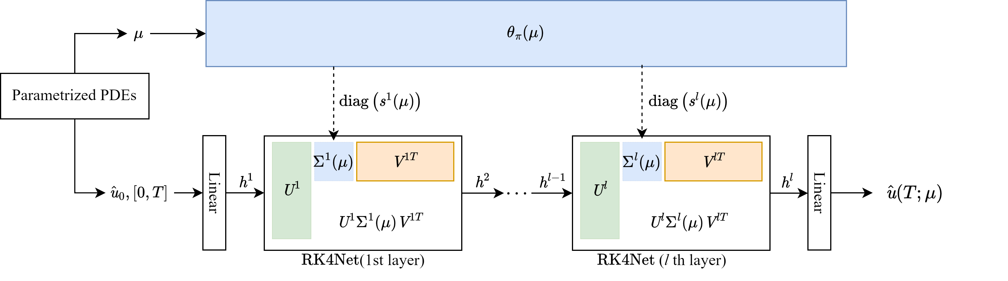
Figure 1: The architecture of HyperPNODE consisting of i) a hypernetwork to generate model parameters (i.e., diagonal elements) and ii) an RK4Net as an integrator for time interval $[0,T]$

Decoder via INR

We decode the latent states using the FourierNet [38], following [31]. It outperforms the other INR architectures in cases without prior knowledge of the PDE and generalizing multiple trajectories. In this setting, the decoder ${\bm{D}}_{{\boldsymbol{\theta}}_{\mathrm{dec}}}$ parametrized by ${\boldsymbol{\theta}}_{\mathrm{dec}}$ is defined as:

$$\tilde{\bm{u}}={\bm{D}}_{{\boldsymbol{\theta}}_{\mathrm{dec}}}(\hat{\bm{u}};{\bm{x}},{\boldsymbol{\theta}}_{\mathrm{dec}}),$$ (7)

where $\tilde{\bm{u}}\in\mathbb{R}^{N_{\bm{u}}}$ are the approximated high-dimensional states for the time interval t. The FourierNet predicts the PDE states at all nodal positions in $\Omega$ and depends on the latent states $\hat{\bm{u}}$.

Training

In this work, we use an auto-decoder in [39] to encode the high-dimensional states into latent space. After the networks are defined, the forward pass of the proposed framework can be summarized as:

1. encode the reduced initial state from given initial condition: $\hat{\bm{u}}_{0}({\boldsymbol{\mu}})={\bm{E}}_{{\boldsymbol{\theta}}_{\mathrm{enc}}}({\bm{u}}_{0}({\boldsymbol{\mu}});{\boldsymbol{\theta}}_{\mathrm{enc}})$

2. learn the latent states $\hat{\bm{u}}$ using PNODE or HyperPNODE

3. decode the collected latent states and use INR to reconstruct high-dimensional states.

4. compute the loss function that consists of data-matching loss and physics-informed loss (PDE residual loss, initial condition loss, and boundary condition loss) [34]

   $$\mathcal{L}=\alpha_{1}\underbrace{\mathrm{MSE}({\bm{u}},\tilde{\bm{u}})}_{\text{data-matching}}+\alpha_{2}\underbrace{\mathrm{MSE}({\bm{r}}(\tilde{\bm{u}}),\mathbf{0})}_{\text{PDE residual}}+\alpha_{3}\underbrace{\mathrm{MSE}(\tilde{\bm{u}}_{0},{\bm{u}}_{0})}_{\text{initial condition}}+\alpha_{4}\underbrace{\mathrm{MSE}(\tilde{\bm{u}}_{\partial\Omega},{\bm{u}}_{\partial\Omega})}_{\text{boundary condition}}$$

   where ${\bm{r}}$ is the residual of the governing equation and $\alpha_{i}$ are user-defined scaling number.

For the training loss, the main loss is the data-matching loss and PDE residual loss can be used as an option. When the PDE residual loss is opted in for training, the methods are denoted by using a name with a suffix, “+PI”. Also, when HyperPNODE is chosen, an additional orthogonality penalty is minimized: $\rho_{1}\|{\bm{U}}^{\mathsf{T}}{}{\bm{U}}-{\bm{I}}\|+\rho_{2}\|{\bm{V}}^{\mathsf{T}}{}{\bm{V}}-{\bm{I}}\|$, where $\rho_{i}$ are the penalty weights.

Fine-tuning INR

As in many other ROM approaches, the proposed method shares the same limitation, performance degradation for unseen PDE parameters (i.e., out-of-distribution samples). To alleviate this limitation, we fine-tune the trained model on a target test PDE parameter in an unsupervised manner by minimizing only the PDE residual loss and selected part of latent dynamics. To this end, we fine-tune the INR with the loss:

$$\mathcal{L}_{\text{ft}}=\beta_{1}\mathrm{MSE}({\bm{r}}(\tilde{\bm{u}}),\mathbf{0})+\beta_{2}\mathrm{MSE}(\tilde{\bm{u}}_{0},{\bm{u}}_{0})+\beta_{3}\mathrm{MSE}(\tilde{\bm{u}}_{\partial\Omega},{\bm{u}}_{\partial\Omega}),$$

where $\beta_{i}$ are penalty weights for PDE residuals, initial condition, and boundary conditions, respectively. Additionally, we fine-tune the hypernetwork since it has a manageable number of parameters.

3 Numerical Results and Discussion

In this section, we apply the proposed INR-ROM method to solve a parametrized computational physics problem adapted from [25]. We demonstrate the effectiveness of the proposed parametric method by comparing the performance with using NODE.

2D Burgers

The problem we consider is solving a two-dimensional, parametrized Burgers’ equation:

$$\frac{\partial{\bm{v}}}{\partial t}=-{\bm{v}}\cdot\nabla{\bm{v}}+\frac{1}{{\boldsymbol{\mu}}}\Delta{\bm{v}},\quad\Omega=[-3,3]\times[-3,3],\quad t\in[0,1],$$ (8)

with the boundary condition ${\bm{v}}({\bm{x}},t;{\boldsymbol{\mu}})=0$ on $\partial\Omega$, an initial condition ${\bm{v}}({\bm{x}},0;{\boldsymbol{\mu}})=0.8e^{-\frac{\norm{{\bm{x}}}^{2}}{1.02}}$ and ${\boldsymbol{\mu}}$ is the Reynolds number used as the PDE parameter. The computational domain has a uniform spatial discretization with $64\times 64$ grid. The full-order model utilizes the implicit backward Euler time integrator with a uniform time step of $\mathit{\Delta}t=1/1000$. In this problem, the training set ${\boldsymbol{\mu}}_{\mathrm{train}}=\left\{30,50,100,500,1000,2000,5000,10000,30000,50000\right\}$, the testing set ${\boldsymbol{\mu}}_{\mathrm{test}}=\left\{20,300,20000,60000\right\}$ are chosen to ensure a large variance on ${\boldsymbol{\mu}}$, which is challenging for the physics-informed neural networks. For each model, we set the dimension of the latent states to be $50$ for each solution component (two components ${\bm{w}}$ and ${\bm{z}}$ in 2D Burgers equation), and ODE MLPs (NODE, PNODE, and RK4Net) to have 3 layers with 256 units per layer. In HyperPNODE, the hypernetwork has only 1 layer with 50 units, and the rank $r=50$ is chosen empirically for reasonable training accuracy. Finally, the learning rate of the INR is $0.01$ and $0.001$ for all other optimizers. We also note that all results shown in this section are the first component ${\bm{w}}$.

We first investigate the performance of different approaches including NODE, PNODE, and HyperPNODE as well as their PI variants on the training set. Table. A1 lists the number of parameters and point-wise relative error to the ground truth values from FOM. Both hypernetworks-based approaches outperform other methods with fewer trainable parameters. Figure. A1 compares the point-wise difference of the PDE states from selected models on the training point $Re=500$. In this parametric setting, NODE fails all cases to predict the ground truth because it minimizes an MSE loss without recording parameter footprints so that it overfits an averaged ${\boldsymbol{\mu}}$ during the training. Hence, we only discuss the accuracy of PNODE and HyperPNODE in the rest of this discussion. After adding physics-informed loss as shown in A2, we observe a slightly larger error for each model. However, we observe that a noisy region is pushed towards the location near discontinuity. This indicates a potential improvement in the physics-informed variants. We cut off the training at 50000 epochs, but a model with PI loss may require further training for better results.

Next, we test the pre-trained model on the test dataset that includes interpolated and extrapolated test values. Table. A2 shows similar results in the training results that adding PI loss can slightly enlarge the error. Meanwhile, the HyperPNODE models have large test errors in low Re cases. Figures A3 and A4 show similar behaviors as in the training results. Adding PI loss increases the maximum error, but it also pushes the error to a reasonable region.

Finally, we fine-tune the model at the test data point, $Re=20$, which introduces the largest relative error. Figure. 2 shows the fine-tuned accuracy by HyperPNODE. The relative test error at $Re=20$ is reduced from 1.234e-01 to 1.005e-01, which is smaller than the result of HyperPNODE without PI loss. In this case, any model without incorporating physics information in the training stage fails this fine-tuning step since it does not record any physics information.

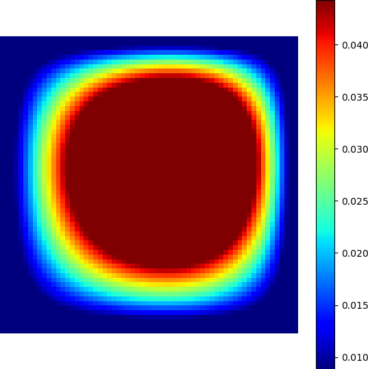
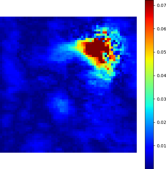
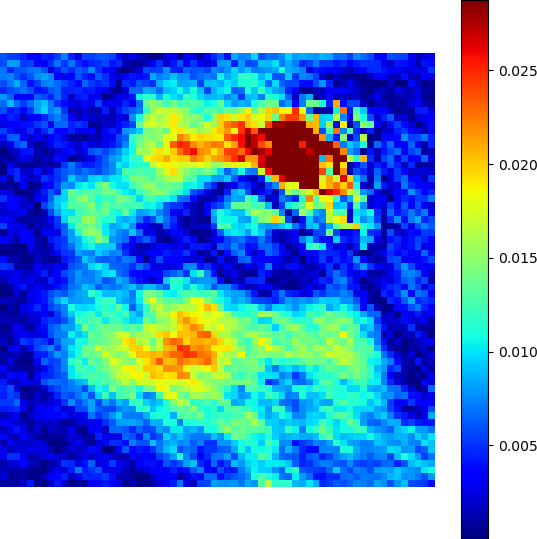
Figure 2: Comparison of point-wise $\norm{{\bm{u}}_{\text{ts}}-\hat{\bm{u}}_{\text{ts}}}$ at $T=1$ for selected $Re=20$ in the testing set. From left to right: reference full order model (FOM) solution, point-wise error between HyperPNODE and FOM, and point-wise error between fine-tuned HyperPNODE and FOM.

Discussion

In this work, we propose a new data-driven reduced-order model inspired by DINo for parametric configurations by using parametrized Neural ODEs (PNODE and HyperPNODE). Both PNODE and HyperPNODE successfully reconstruct the FOM solutions and provide reasonable solutions on unseen PDE parameters. With all variances of the proposed framework, we obtain $\sim 1\%$ averaged relative error on the training set, and $\sim 4\%$ averaged error on the test set. Different models with their PINN variants have a similar range of speedups from $\mathcal{O}(10^{2})$ to $\mathcal{O}(10^{3})$. We also employ an unsupervised fine-tuning method to improve the worst scenario of the HyperPNODE+PI loss model by reducing $\sim 2\%$ of the error.

Future direction

There are potential improvements to the current PINN variants, including tailoring the FouriNet for spatial-temporal inputs, additional training stage, and reducing the overfitting issue in HyerPNODE models.

4 Broader impact

This paper introduces a new data-driven parametrized reduced-order-modeling technique using INR as a decoder to reconstruct data at a continuous level. The proposed INR-ROM framework is expected to have broad impacts on the computational science community and application potentials in a wide range of engineering and scientific domains. There is no negative consequence on ethics and society in this work.

Appendix: Additional Figures and Tables

Table A1: Comparison of the number of trainable parameters and the training accuracy

Model	# Parameters	Avg. $\frac{\norm{{\bm{u}}_{\text{tr}}-\hat{\bm{u}}_{\text{tr}}}}{\norm{{\bm{u}}_{\text{tr}}}}$	Max. $\frac{\norm{{\bm{u}}_{\text{tr}}-\hat{\bm{u}}_{\text{tr}}}}{\norm{{\bm{u}}_{\text{tr}}}}$
NODE	209128	1.798e-01	4.802e-01
NODE+PI	209128	1.798e-01	4.801e-01
PNODE	209641	1.094e-02	1.459e-02
PNODE+PI	209641	1.430e-02	1.931e-02
HyerPNODE	165509	8.336e-03	1.068e-02
HyerPNODE+PI	165509	1.140e-02	1.421e-02

Table A2: Comparison of the test accuracy and speedups

Model	Avg. $\frac{\norm{{\bm{u}}_{\text{ts}}-\hat{\bm{u}}_{\text{ts}}}}{\norm{{\bm{u}}_{\text{ts}}}}$	Max. $\frac{\norm{{\bm{u}}_{\text{ts}}-\hat{\bm{u}}_{\text{ts}}}}{\norm{{\bm{u}}_{\text{ts}}}}$	Min. Speedup	Max. Speedup
NODE	2.653e-01	6.821e-01	1.133e+02	1.320e+03
NODE+PI	2.654e-01	6.819e-01	1.142e+02	1.364e+03
PNODE	3.212e-02	7.487e-02	1.164e+02	1.292e+03
PNODE+PI	4.861e-02	1.099e-01	1.151e+02	1.280e+03
HyerPNODE	4.537e-02	1.238e-01	1.173e+02	1.832e+03
HyerPNODE+PI	4.618e-02	1.234e-01	1.167e+02	1.811e+03

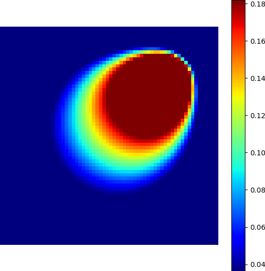
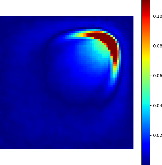
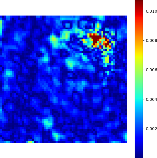
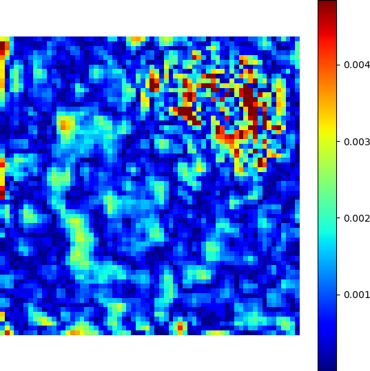
Figure A1: From left to right: FOM reference solution and the comparison of point-wise $\norm{{\bm{u}}_{\text{tr}}-\hat{\bm{u}}_{\text{tr}}}$ at $T=1$ and selected $Re=500$ in the training set for NODE, PNODE, and HyperPNODE, respectively.

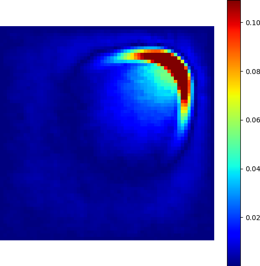
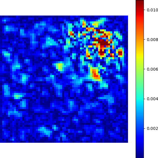
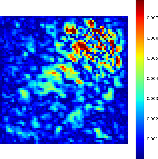
Figure A2: From left to right: FOM reference solution and the comparison of point-wise $\norm{{\bm{u}}_{\text{tr}}-\hat{\bm{u}}_{\text{tr}}}$ at $T=1$ and selected $Re=500$ in the training set for NODE+PI, PNODE+PI, and HyperPNODE+PI, respectively.

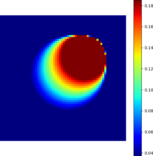
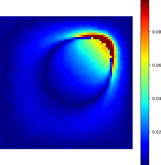
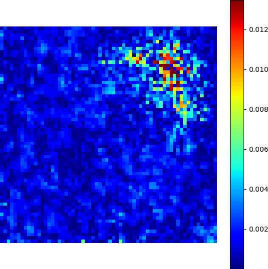
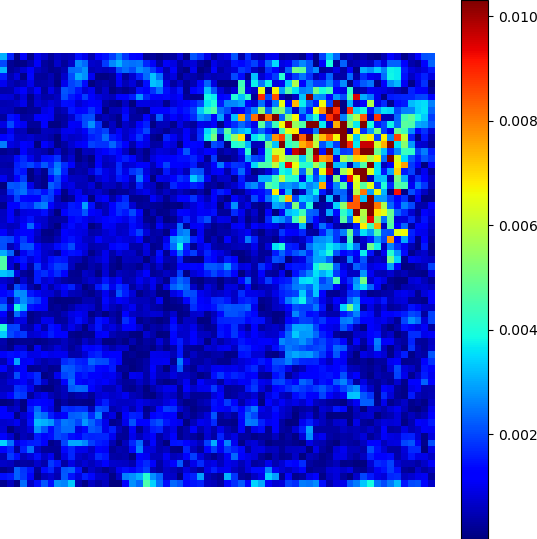
Figure A3: From left to right: FOM reference solution and the comparison of point-wise $\norm{{\bm{u}}_{\text{ts}}-\hat{\bm{u}}_{\text{ts}}}$ at $T=1$ and selected $Re=60000$ in the training set for NODE, PNODE, and HyperPNODE, respectively.

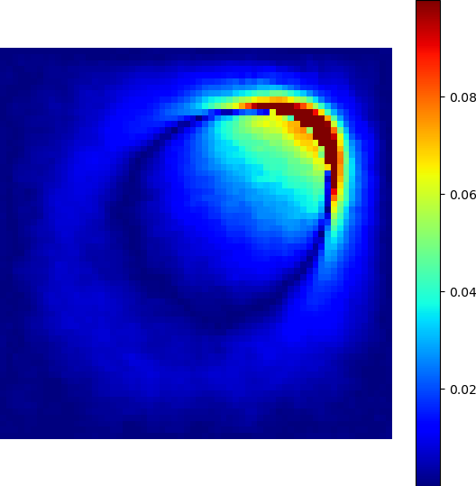
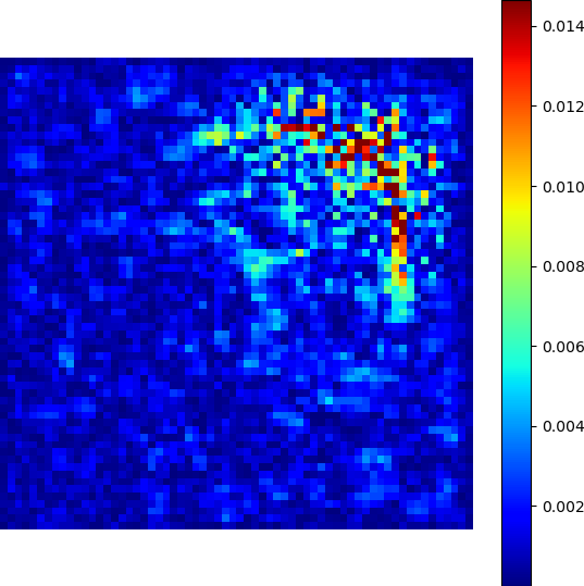
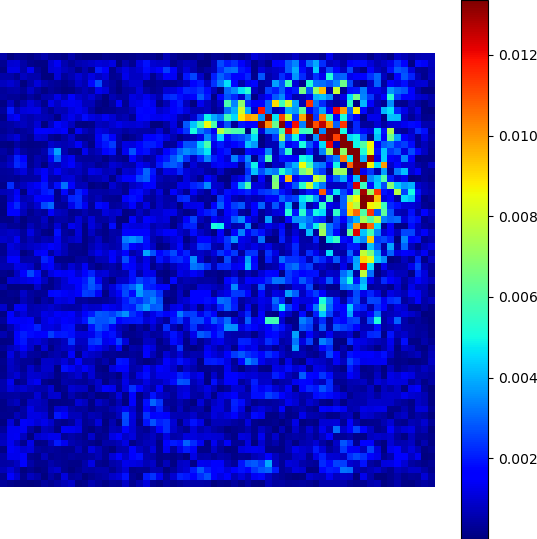
Figure A4: From left to right: FOM reference solution and the comparison of point-wise $\norm{{\bm{u}}_{\text{ts}}-\hat{\bm{u}}_{\text{ts}}}$ at $T=1$ and selected $Re=60000$ in the training set for NODE+PI, PNODE+PI, and HyperPNODE+PI, respectively.

References

- [1] Matthew J. Zahr and Charbel Farhat. Progressive construction of a parametric reduced-order model for PDE-constrained optimization. International Journal for Numerical Methods in Engineering, 102(5):1111–1135, May 2015.
- [2] Eyal Arian, Marco Fahl, and Ekkehard W. Sachs. Trust-region proper orthogonal decomposition for flow control.
- [3] Elizabeth Qian, Martin Grepl, Karen Veroy, and Karen Willcox. A Certified Trust Region Reduced Basis Approach to PDE-Constrained Optimization. SIAM Journal on Scientific Computing, 39(5):S434–S460, January 2017.
- [4] Youngsoo Choi, Gabriele Boncoraglio, Spenser Anderson, David Amsallem, and Charbel Farhat. Gradient-based constrained optimization using a database of linear reduced-order models. Journal of Computational Physics, 423:109787, 2020.
- [5] Masayuki Yano, Tianci Huang, and Matthew J. Zahr. A globally convergent method to accelerate topology optimization using on-the-fly model reduction. Computer Methods in Applied Mechanics and Engineering, 375:113635, March 2021.
- [6] Sean McBane, Youngsoo Choi, and Karen Willcox. Stress-constrained topology optimization of lattice-like structures using component-wise reduced order models. Computer Methods in Applied Mechanics and Engineering, 400:115525, 2022.
- [7] Tianshu Wen and Matthew J. Zahr. A globally convergent method to accelerate large-scale optimization using on-the-fly model hyperreduction: Application to shape optimization. Journal of Computational Physics, 484:112082, July 2023.
- [8] Kevin Carlberg, Youngsoo Choi, and Syuzanna Sargsyan. Conservative model reduction for finite-volume models. Journal of Computational Physics, 371:280–314, 2018.
- [9] Siu Wun Cheung, Youngsoo Choi, H. Keo Springer, and Teeratorn Kadeethum. Data-scarce surrogate modeling of shock-induced pore collapse process. 2023.
- [10] Jessica T Lauzon, Siu Wun Cheung, Yeonjong Shin, Youngsoo Choi, Dylan Matthew Copeland, and Kevin Huynh. S-opt: A points selection algorithm for hyper-reduction in reduced order models. arXiv preprint arXiv:2203.16494, 2022.
- [11] Ping-Hsuan Tsai, Seung Whan Chung, Debojyoti Ghosh, John Loffeld, Youngsoo Choi, and Jonathan L. Belof. Accelerating kinetic simulations of electrostatic plasmas with reduced-order modeling. 2023.
- [12] Youngkyu Kim, Karen Wang, and Youngsoo Choi. Efficient space–time reduced order model for linear dynamical systems in python using less than 120 lines of code. Mathematics, 9(14):1690, 2021.
- [13] Dylan Matthew Copeland, Siu Wun Cheung, Kevin Huynh, and Youngsoo Choi. Reduced order models for lagrangian hydrodynamics. Computer Methods in Applied Mechanics and Engineering, 388:114259, 2022.
- [14] Quincy A Huhn, Mauricio E Tano, Jean C Ragusa, and Youngsoo Choi. Parametric dynamic mode decomposition for reduced order modeling. Journal of Computational Physics, 475:111852, 2023.
- [15] Youngsoo Choi, Deshawn Coombs, and Robert Anderson. Sns: A solution-based nonlinear subspace method for time-dependent model order reduction. SIAM Journal on Scientific Computing, 42(2):A1116–A1146, 2020.
- [16] Siu Wun Cheung, Youngsoo Choi, Dylan Matthew Copeland, and Kevin Huynh. Local lagrangian reduced-order modeling for the rayleigh-taylor instability by solution manifold decomposition. Journal of Computational Physics, 472:111655, 2023.
- [17] Sean McBane and Youngsoo Choi. Component-wise reduced order model lattice-type structure design. Computer methods in applied mechanics and engineering, 381:113813, 2021.
- [18] Chi Hoang, Youngsoo Choi, and Kevin Carlberg. Domain-decomposition least-squares petrov–galerkin (dd-lspg) nonlinear model reduction. Computer methods in applied mechanics and engineering, 384:113997, 2021.
- [19] Youngsoo Choi and Kevin Carlberg. Space–time least-squares petrov–galerkin projection for nonlinear model reduction. SIAM Journal on Scientific Computing, 41(1):A26–A58, 2019.
- [20] Renee Swischuk, Laura Mainini, Benjamin Peherstorfer, and Karen Willcox. Projection-based model reduction: Formulations for physics-based machine learning. 179:704–717.
- [21] Kookjin Lee and Kevin T Carlberg. Model reduction of dynamical systems on nonlinear manifolds using deep convolutional autoencoders. Journal of Computational Physics, 404:108973, 2020.
- [22] Kookjin Lee and Kevin T Carlberg. Deep conservation: A latent-dynamics model for exact satisfaction of physical conservation laws. In Proceedings of the AAAI Conference on Artificial Intelligence, volume 35, pages 277–285, 2021.
- [23] Youngkyu Kim, Youngsoo Choi, David Widemann, and Tarek Zohdi. Efficient nonlinear manifold reduced order model. arXiv preprint arXiv:2011.07727, 2020.
- [24] Youngkyu Kim, Youngsoo Choi, David Widemann, and Tarek Zohdi. A fast and accurate physics-informed neural network reduced order model with shallow masked autoencoder. Journal of Computational Physics, 451:110841, 2022.
- [25] William D. Fries, Xiaolong He, and Youngsoo Choi. LaSDI: Parametric latent space dynamics identification. 399:115436.
- [26] T. Kadeethum, F. Ballarin, Y. Choi, D. O’Malley, H. Yoon, and N. Bouklas. Non-intrusive reduced order modeling of natural convection in porous media using convolutional autoencoders: Comparison with linear subspace techniques. 160:104098.
- [27] Xiaolong He, Youngsoo Choi, William D. Fries, Jonathan L. Belof, and Jiun-Shyan Chen. gLaSDI: Parametric physics-informed greedy latent space dynamics identification. 489:112267.
- [28] Joshua Barnett, Charbel Farhat, and Yvon Maday. Neural-network-augmented projection-based model order reduction for mitigating the kolmogorov barrier to reducibility. 492:112420.
- [29] Peter Yichen Chen, Jinxu Xiang, Dong Heon Cho, Yue Chang, GA Pershing, Henrique Teles Maia, Maurizio Chiaramonte, Kevin Carlberg, and Eitan Grinspun. Crom: Continuous reduced-order modeling of pdes using implicit neural representations. arXiv preprint arXiv:2206.02607, 2022.
- [30] Zhong Yi Wan, Leonardo Zepeda-Nunez, Anudhyan Boral, and Fei Sha. Evolve smoothly, fit consistently: Learning smooth latent dynamics for advection-dominated systems. In The Eleventh International Conference on Learning Representations, 2023.
- [31] Yuan Yin, Matthieu Kirchmeyer, Jean-Yves Franceschi, Alain Rakotomamonjy, and Patrick Gallinari. Continuous PDE dynamics forecasting with implicit neural representations.
- [32] Ricky TQ Chen, Yulia Rubanova, Jesse Bettencourt, and David K Duvenaud. Neural ordinary differential equations. Advances in neural information processing systems, 31, 2018.
- [33] Kookjin Lee and Eric J. Parish. Parameterized neural ordinary differential equations: Applications to computational physics problems. 477(2253):20210162.
- [34] Maziar Raissi, Paris Perdikaris, and George E Karniadakis. Physics-informed neural networks: A deep learning framework for solving forward and inverse problems involving nonlinear partial differential equations. Journal of Computational physics, 378:686–707, 2019.
- [35] Christophe Bonneville, Youngsoo Choi, Debojyoti Ghosh, and Jonathan L Belof. Gplasdi: Gaussian process-based interpretable latent space dynamics identification through deep autoencoder. Computer Methods in Applied Mechanics and Engineering, 418:116535, 2024.
- [36] April Tran, Xiaolong He, Daniel A. Messenger, Youngsoo Choi, and David M. Bortz. Weak-form latent space dynamics identification. 2023.
- [37] Aditi S. Krishnapriyan, Alejandro F. Queiruga, N. Benjamin Erichson, and Michael W. Mahoney. Learning continuous models for continuous physics.
- [38] Rizal Fathony, Devin Willmott, Anit Kumar Sahu, and J Zico Kolter. MULTIPLICATIVE FILTER NETWORKS.
- [39] Jeong Joon Park, Peter Florence, Julian Straub, Richard Newcombe, and Steven Lovegrove. DeepSDF: Learning continuous signed distance functions for shape representation.