Learning Multimodal Latent Dynamics for Human-Robot Interaction

Abstract

This article presents a method for learning well-coordinated Human-Robot Interaction (HRI) from Human-Human Interactions (HHI). We devise a hybrid approach using Hidden Markov Models (HMMs) as the latent space priors for a Variational Autoencoder to model a joint distribution over the interacting agents. We leverage the interaction dynamics learned from HHI to learn HRI and incorporate the conditional generation of robot motions from human observations into the training, thereby predicting more accurate robot trajectories. The generated robot motions are further adapted with Inverse Kinematics to ensure the desired physical proximity with a human, combining the ease of joint space learning and accurate task space reachability. For contact-rich interactions, we modulate the robot’s stiffness using HMM segmentation for a compliant interaction. We verify the effectiveness of our approach deployed on a Humanoid robot via a user study. Our method generalizes well to various humans despite being trained on data from just two humans. We find that Users perceive our method as more human-like, timely, and accurate and rank our method with a higher degree of preference over other baselines.

I Introduction

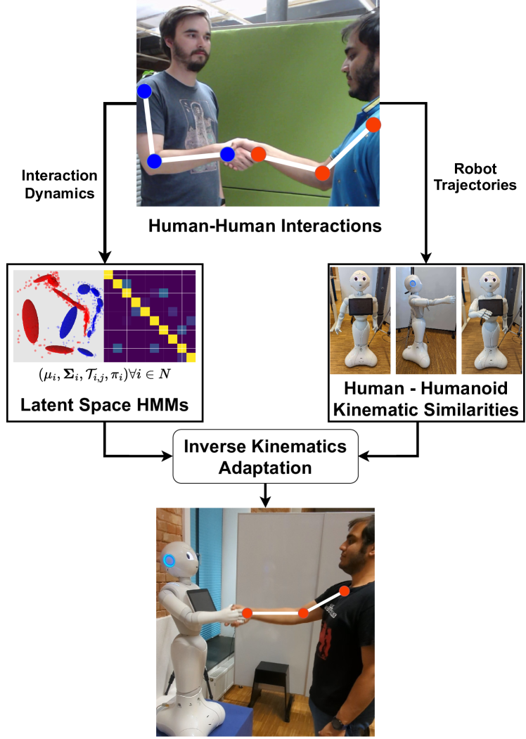
Figure 1: We explore learning coordinated HRI behaviors using Hidden Markov Models (HMMs) to learn the interaction dynamics over a representation space spanned by a Variational Autoencoder (VAE). The VAEs are trained with the HMMs as a prior to better incorporate the understanding of the dynamics. Moreover, we learn directly from Human-Human interactions by leveraging the kinematic similarities of Humans and Humanoid robots. During testing, the predicted trajectories are adapted with Inverse Kinematics to mitigate errors in the spatial accuracy arising either from prediction errors or from shortcomings in transferring the human’s actions to the robot.

Ensuring a synchronized and accurate reaction is an important aspect in Human-Robot Interaction (HRI) [3]. To do so, a human and a robot need to spatiotemporally coordinate their movements to reach a common target or perform a common task, that can be denoted as a joint action [72]. For realizing such coordinated jointly performed actions, spatial and temporal adaptation of motions in the shared physical space to accurately perform the action are key factors [73]. Such interpersonal coordination can enable a connection to one’s interaction partner [52].

Therefore, well-executed and well-coordinated interactive behaviors can improve the perception of a social robot.

The paradigm of Learning from Demonstrations (LfD) is promising for HRI by learning joint distributions over human and robot trajectories in a modular, multimodal manner [28, 15, 64, 29, 41]. However, LfD approaches scale poorly with higher dimensions, which can be circumvented by incorporating Deep Learning for learning latent-space dynamics. Such Deep State-Space Models have shown good performance in capturing temporal dependencies of latent space trajectories, either using some kind of a forward propagation model [8, 25, 23, 13], learning the parameters for a dynamics model with LfD [39, 22, 20] or fitting parameterized LfD models to the underlying latent trajectories [27, 54]. In this paper, we further explore this direction of latent space dynamics in the context of Human-Robot Interaction.

Furthermore, when learning trajectories in the joint configuration space of a robot, minor deviations in the joint space can cause a perceivable deviation in the robot’s task space. While learning task space trajectories can mitigate problems from errors in the joint space, to do so, the demonstrated trajectories need to fall within the reachability of the robot. When this reachability assumption is violated, the task space proximity in HRI scenarios may not be effectively learned. Moreover, learning purely task space trajectories doesn’t necessarily ensure human-like joint configurations, which is especially relevant for Humanoid robots. To this end, the combination of joint space learning and task space reachability can be achieved using Inverse Kinematics to supplement the learned behaviors [33, 66, 18].

In this paper, as shown in Figure 1, we are interested in learning and adapting Deep LfD policies for spatiotemporally coherent interactive behaviors. We learn the interaction dynamics from HHI demonstrations using latent space Hidden Markov Models (HMMs). We show the efficacy of the learnt dynamics in real-world HRI scenarios. We do so in a manner that ensures spatially accurate physical proximity to the human partner and additionally enable compliant robot motions in contact-rich interactions like a handshake, thereby improving the perceived quality of the HRI behaviors.

I-A Related Work

I-A1 Learning HRI from Demonstrations

Early approaches for learning modular HRI policies modeled the interaction as a joint distribution with a Gaussian Mixture Model (GMM) learned over demonstrated trajectories of a human and a robot in a collaborative task [15]. The correlations between the human and the robot degrees of freedom (DoFs) can then be leveraged to generate the robot’s trajectory given observations of the human for learning both proactive and reactive controllers [70, 14, 64]. Segmenting HRI demonstrations has also been shown using Graphical Models with Markov chain Monte Carlo [77, 76].

Along the lines of leveraging Gaussian approximations for LfD, Movement Primitives [62], which learn a distribution over underlying linear regression weight vectors, were extended for HRI by similarly learning a joint distribution over the weights of interacting agents [5, 49, 16]. Movement Primitive approaches can further be combined with GMMs for learning multiple task sequences seamlessly [29, 50, 41, 59, 45]. One drawback of the aforementioned primitive-based approaches is that they do not perform well on out-of-distribution data [87]. Additionally, for tasks that are loosely coupled in time, Movement Primitives can underperform [61]. These drawbacks therefore make them an unviable option for being able to generalize spatiotemporally in interactive behaviors. For a more extensive overview of Movement Primitive approaches for robot learning, we refer the reader to [81].

Vogt et al. [84] are similar in theory to our approach where they learn the interaction dynamics of Human-Human Interactions using an HMM over a low dimensional representation space of the human skeletons. In our approach, we show further performance improvements by incorporating human-conditioned reactive motion generation into the training pipeline.Additionally, Vogt et al. [84] train Interaction Meshes [37] for transferring the learned trajectories to a robot whose prediction is optimized during runtime to adapt to the human user’s movements. As we work with Humanoid Robots, we follow a simpler approach by leveraging the structural similarity between a human and a humanoid. This allows us to map the joint motions directly [31] and adapt the motions to the interaction partner using Inverse Kinematics [66]. Through our user study, we find that our approach, while being simplistic, provides acceptable interactions with various human partners.

To make the learned distribution more robust, LfD methods are often learned via kinesthetic teaching which can be tedious for HRI tasks where one would need a variety of human partners. The need for extensive training data can potentially be circumvented by learning how humans adapt to a robot’s trajectory [17]. A more general way, especially in the context of Humanoid robots, is by learning from human-human demonstrations by leveraging the kinematic similarities between humans and robots [31]. While such approaches of motion retargeting leave some room for error due to minor differences between human and robot geometries, adapting the trajectories in the robot’s task space via Inverse Kinematics can improve the accuracy of such interactive behaviors [66, 82].

I-A2 Integrating LfD with Deep Learning

Techniques at the intersection of LfD coupled with the use of Neural Network representations for higher dimensional data have grown in popularity for learning latent trajectory dynamics from demonstrations. Typically, an autoencoding approach, like VAEs, is used to encode latent trajectories over which a latent dynamics model is trained. In their simplest form, the latent dynamics can be modeled either with linear Gaussian models [39] or Kalman filters [8]. Other approaches learn stable dynamical systems, like Dynamic Movement Primitives [71] over VAE latent spaces [10, 21, 22, 20, 24]. Instead of learning a feedforward dynamics model, Dermy et al. [27] model the entire trajectory’s dynamics at once using Probabilistic Movement Primitives [62] achieving better results than [20].

Nagano et al. [54] demonstrated the use of Hidden Semi-Markov Models (HSMMs) as latent priors in a VAE for temporal action segmentation of motions involving a single human. They model each latent dimension independently, which is not favorable when learning interaction dynamics. To extend such an approach for learning HRI, one needs to consider the interdependence between dimensions. In our previous work, “MILD” [65], we extend this idea of using HSMMs as VAE priors for interactive tasks by exploiting the full rank of HSMM covariance matrices thereby capturing the dependencies between both agents by learning a joint distribution over the latent trajectories of interacting partners.

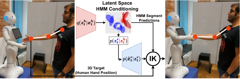
Figure 2: Overview of our approach. We train VAEs to reconstruct the observations of the interactions agents $(\boldsymbol{x}^{h}_{1:t},\boldsymbol{x}^{r}_{1:t})$ with an HMM prior to learn a joint distribution over the latent space trajectories $p(\boldsymbol{z}^{h}_{1:t},\boldsymbol{z}^{r}_{1:t})$ of the interacting agents. During test time, the observed agent’s latent trajectory conditions the HMM to infer the robot agent’s latent trajectory $p(\boldsymbol{z}^{r}_{t}|\boldsymbol{z}^{h}_{1:t})$ which is decoded to generate the robot agent’s joint trajectory $\boldsymbol{\hat{x}}^{r}_{t}$. To ensure the proximity of a robot’s hand to the human’s hand during test time, we additionally adapt the predicted trajectory using Inverse Kinematics to fulfill the contact-based nature of the interaction.

I-A3 Interaction Modeling with Recurrent Neural Networks

When large datasets are available, Recurrent latent space models are powerful tools in approximating latent dynamics with some form of a forward propagating distribution [23, 34, 42, 46, 30]. Given their power of modeling temporal sequences, they yield themselves naturally for learning interactive/collaborative tasks in HRI [58, 86, 74]. To simplify the various scenarios of interaction tasks Oguz et al. [58] develop an ontology to categorize interaction scenarios and train an LSTM network for each case in a simple Imitation Learning paradigm. Similarly, Zhao et al. [86] explore using such LSTM-based policies for learning HRI in a simple collaboration scenario. Rather than simply regressing robot actions to human inputs, Bütepage et al. [13] explore the idea of learning shared latent dynamics in HRI in a systematic way. They first learn latent embeddings of the human and robot motions individually using a VAE following which the latent interaction dynamics of Human-Human Interactions (HHI) in learned using LSTMs. The learned HHI dynamics are used in conjunction with the learned robot embeddings to subsequently learn the robot dynamics from HRI demonstrations. However, we find in our experiments that the autoregressive nature of their approach, unfortunately, leads to a divergence in the performance since they only train it using ground truth demonstrations and not in an autoregressive manner. In contrast, rather than having an implicit shared representation, such as with an LSTM, the LfD approaches can be explicitly conditioned on the interaction partner’s observations [5, 28] which we find leads to improved predictive performance.

I-A4 Unsupervised Skill Discovery

While skill discovery is not the main focus of our approach, there are some parallels between our approach and works on unsupervised skill discovery which we discuss below. In general, such approaches aim to partition a latent space into different skills which can then be sequenced for learning a variety of different tasks either from demonstrations or using Reinforcement Learning (an overview can be found in Sec. III-B in [53]). The works closest to our approach [80, 55, 68] explore this key idea of learning how to segment demonstrations into underlying recurring segments or “skills” by decomposing a latent representation of the trajectories and subsequently learning the temporal relations between these skills to compose the observed trajectories. Similar approaches are further explored in literature using different skill representations such as the Options framework [75] or Autoregressive HMMs [57, 44]. While the main focus of such approaches is the decomposition of demonstrations to learn re-usable atomic “skills”, our main aim is to explore how to do so in HRI settings via a joint distribution over the actions of interacting partners and subsequently how the learned skills/segments can be inferred during test time based on the dynamic observations of a human, rather than reproducing a given task or based on a static goal.

I-B Objectives and Contributions

In our previous work [65] on learning Multimodal Interactive Latent Dynamics, “MILD”, we explored how Deep LfD can be used for learning spatiotemporally coherent interaction dynamics. Rather than using an uninformed, stationary prior for learning HRI [13], we showed the use of Hidden Semi-Markov Models to model the latent space prior of a VAE as a joint distribution over the trajectories of both interacting agents. During test time, the robot trajectories can be conditionally generated based on the observed human trajectories in the latent space, showing that such an approach can capture the latent interaction dynamics suitably well. In this article, we extend MILD [65] by systematically improving the predictive abilities of our model by incorporating reactive motion generation into the training process. We do so by exploring two different sampling approaches to incorporate the conditional distribution of the HMM into the training, rather than using the HMM just as a VAE prior as done in [65]. Furthermore, to deploy the proposed approach on the Humanoid Social Robot Pepper [60], we leverage the similarity between the kinematic structures of Pepper and a Human to effectively learn HRI behaviors from Human-Human Interactions. We further show how the predictions from the latent space HMMs can help supplement the robot controller by modulating the target motions via Inverse Kinematics for a more accurate interaction and modulating the joint stiffnesses for ensuring compliant motions during a contact-rich interaction like a handshake (Figure 2).

Specifically, our contributions beyond MILD [65] are summarized below:

1. We systematically explore how to incorporate human-conditioned reactive motion generation of the robot trajectories in the training to improve the prediction accuracy of our model.

2. We integrate Inverse Kinematics in our pipeline to spatially adapt the predicted robot motions to the interaction partner, thereby ensuring suitable physical proximity and improved spatial accuracy of the learned behaviors.

3. For contact-rich interactions like handshaking, we perform stiffness modulation using the HMM’s segment predictions to enable realistic and compliant robot motions.

4. We validate our approach via a user study where participants interact with a Pepper robot controlled by our approach. We find that our method ranks highly compared to other baselines and provides a perceivably more human-like, natural, timely, and accurate interaction, thereby showcasing its effectiveness.

The rest of the paper is organized as follows. In Section II, we explain the foundations needed to understand our work. We then explain our approach in Section III. We highlight our experiments and results in Section IV and present some concluding remarks and directions for future work in Section V.

II Foundations

We first explain Variational Autoencoders (VAEs) (Section II-A) which is the main backbone of our approach, followed by Hidden Markov Models (HMMs) (Section II-B), which are key for learning the interaction dynamics, and finally, we give an introduction to Inverse Kinematics (IK) (Sec II-C) which is essential for improving the overall acceptance of our approach.

II-A Variational Autoencoders

Variational Autoencoders (VAEs) [40, 69] are a type of neural network architecture that learns the identity function in an unsupervised, probabilistic way. The inputs “$\boldsymbol{x}$” are encoded into lower dimensional latent space embeddings “$\boldsymbol{z}$” that a decoder uses to reconstruct the original input. A prior distribution is enforced over the latent space during the learning, which is typically a standard normal distribution $p(\boldsymbol{z})=\mathcal{N}(\boldsymbol{z};\boldsymbol{0,I})$. The goal is to estimate the true posterior $p(\boldsymbol{z|x})$, using a neural network $q(\boldsymbol{z|x})$ and is trained by minimizing the Kullback-Leibler (KL) divergence between them

$$KL(q(\boldsymbol{z|x})||p(\boldsymbol{z|x}))=\mathbb{E}_{q}[\log\frac{q(\boldsymbol{z|x})}{p(\boldsymbol{x,z})}]+\log p(\boldsymbol{x})$$ (1)

which can be re-written as

$$\log p(\boldsymbol{x})=KL(q(\boldsymbol{z|x})||p(\boldsymbol{z|x}))+\mathbb{E}_{q}[\log\frac{p(\boldsymbol{x,z})}{q(\boldsymbol{z|x})}].$$ (2)

The KL divergence is always non-negative, therefore the second term in Eq. 2 acts as a lower bound. Maximizing it would effectively maximize the log-likelihood of the data distribution or evidence, and is hence called the Evidence Lower Bound (ELBO), which can be written as

$$\mathbb{E}_{q}[\log\frac{p(\boldsymbol{x,z})}{q(\boldsymbol{z|x})}]=\mathbb{E}_{q}[\log p(\boldsymbol{x|z})]-\beta KL(q(\boldsymbol{z|x})||p(\boldsymbol{z})).$$ (3)

The first term aims to reconstruct the input via samples decoded from the posterior. The second term is the KL divergence between the prior and the posterior, which regularizes the learning. To prevent over-regularization, the KL divergence term is also weighted down with a factor $\beta$. Further information can be found in [40, 69, 35].

II-B Hidden Markov Models

A Hidden Markov Model (HMM) is used to model a sequence of observations $\boldsymbol{z}_{1:T}$ (robot joint angles, human skeletons, etc.) as a sequence of underlying hidden states such that they can “emit” the observations with a given probability. In mathematical terms, an HMM is characterized by a set of hidden states $i\in\{1,2\dots N\}$, each of which denotes a probability distribution, in our case a Gaussian with mean $\boldsymbol{\mu}_{i}$ and covariance $\boldsymbol{\Sigma}_{i}$, which characterize the emission probabilities of observations $\mathcal{N}(\boldsymbol{z}_{t};\boldsymbol{\mu}_{i},\boldsymbol{\Sigma}_{i})$. An initial state distribution $\pi_{i}$ denotes the initial probabilities of being in each state, and the state transition probabilities $\mathcal{T}_{i,j}$ describe the probability of the model going from the $i^{th}$ state to the $j^{th}$ state. The sequential progression via the probability of each hidden state given an observed sequence $\boldsymbol{z}_{1:t}$ is denoted by the forward variable of the HMM $\alpha_{i}(\boldsymbol{z}_{t})$

$$\begin{gathered}\alpha_{i}(\boldsymbol{z}_{t})=\frac{\hat{\alpha}_{i}(\boldsymbol{z}_{t})}{\sum\nolimits_{j=1}^{N}\hat{\alpha}_{j}(\boldsymbol{z}_{t})}\\ \hat{\alpha}_{i}(\boldsymbol{z}_{t})=\mathcal{N}(\boldsymbol{z}_{t};\boldsymbol{\mu}_{i},\boldsymbol{\Sigma}_{i})\sum_{j=1}^{N}\alpha_{j}(\boldsymbol{z}_{t-1})\mathcal{T}_{j,i}\\ \hat{\alpha}_{i}(\boldsymbol{z}_{0})=\pi_{i}\hskip 1.99997pt\mathcal{N}(\boldsymbol{z}_{0};\boldsymbol{\mu}_{i},\boldsymbol{\Sigma}_{i})\end{gathered}$$ (4)

where $\hat{\alpha}_{i}(\boldsymbol{z}_{t})$ represents the non-normalized forward variable and $\pi_{i}$ is the initial state distribution.

The HMM is trained using Expectation-Maximization over the parameters $(\pi_{i},\boldsymbol{\mu}_{i},\boldsymbol{\Sigma}_{i},\mathcal{T}_{j,i})$ with the trajectory data. We refer the reader to [14, 64] for further details on HMMs in the context of robot learning.

In HRI scenarios, to encode the joint distribution between the human and the robot, we concatenate the Degrees of Freedom (DoFs) of both the human and the robot [15, 28] allowing the distribution to be decomposed as

$$\boldsymbol{\mu}_{i}=\begin{bmatrix}\boldsymbol{\mu}^{h}_{i}\\ \boldsymbol{\mu}^{r}_{i}\end{bmatrix};\boldsymbol{\Sigma}_{i}=\begin{bmatrix}\boldsymbol{\Sigma}^{hh}_{i}&\boldsymbol{\Sigma}^{hr}_{i}\\ \boldsymbol{\Sigma}^{rh}_{i}&\boldsymbol{\Sigma}^{rr}_{i}\end{bmatrix}$$ (5)

where the superscript indicates the different agents ($h$-human, $r$-robot). Once the distributions are learned, given some observations of the human agent $\boldsymbol{z}^{h}_{t}$, the robot’s trajectory can be conditionally generated using Gaussian Mixture Regression as

$$\boldsymbol{K}_{i} =\boldsymbol{\Sigma}^{rh}_{i}(\boldsymbol{\Sigma}^{hh}_{i})^{-1}$$ (6)

$$\boldsymbol{\hat{\mu}}^{r}_{i} =\boldsymbol{\mu}^{r}_{i}+\boldsymbol{K}_{i}(\boldsymbol{z}^{h}_{t}-\boldsymbol{\mu}^{h}_{i})$$ (7)

$$\boldsymbol{\hat{\Sigma}}^{r}_{i} =\boldsymbol{\Sigma}^{rr}_{i}-\boldsymbol{K}_{i}\boldsymbol{\Sigma}^{hr}_{i}+\boldsymbol{\hat{\mu}}^{r}_{i}(\boldsymbol{\hat{\mu}}^{r}_{i})^{T}$$ (8)

$$\boldsymbol{\hat{\mu}}^{r}_{t} =\sum_{i=1}^{N}\alpha_{i}(\boldsymbol{z}^{h}_{t})\boldsymbol{\hat{\mu}}^{r}_{i}$$ (9)

$$\boldsymbol{\hat{\Sigma}}^{r}_{t} =\sum_{i=1}^{N}\alpha_{i}(\boldsymbol{z}^{h}_{t})\boldsymbol{\hat{\Sigma}}^{r}_{i}-\boldsymbol{\hat{\mu}}^{r}_{t}(\boldsymbol{\hat{\mu}}^{r}_{t})^{T}$$ (10)

$$p(\boldsymbol{z}^{r}_{t}|\boldsymbol{z}^{h}_{t}) =\mathcal{N}(\boldsymbol{z}^{r}_{t}|\boldsymbol{\hat{\mu}}^{r}_{t},\boldsymbol{\hat{\Sigma}}^{r}_{t})$$ (11)

where $\alpha_{i}(\boldsymbol{z}^{h}_{t})$ is the forward variable calculated using the marginal distribution of the observed human agent.

II-C Inverse Kinematics

Given a joint angle configuration $\boldsymbol{y}$, the end effector position can be calculated as $\boldsymbol{x}_{ee}=f(\boldsymbol{y})$ where $f(\boldsymbol{y})$ denotes the forward kinematics of the robot, which is based on the robot’s geometry and calculates the end effector position through the hierarchy of intermediate transformations of each of the individual joints. For example, given the geometry of one’s arm sizes, and the angles of the shoulder, elbow, and wrist joints, the position of the hand can be calculated through the position of the shoulder to the elbow to the hand.

Given a list of $n$ joints $\boldsymbol{y}=\{y_{1},y_{2}\ldots y_{n}\}$ and the corresponding relative transformations that the joints represent in the robot geometry $\boldsymbol{T}^{0}_{1}(y_{1}),\boldsymbol{T}^{1}_{2}(y_{2})\ldots\boldsymbol{T}^{n-1}_{n}(y_{n})$ where $\boldsymbol{T}^{i}_{j}\in SE(3)$ is the relative transformation between links $i$ and $j$, the end effector pose $\boldsymbol{T}_{ee}$ can be calculated as

$$\boldsymbol{T}_{ee}=\begin{bmatrix}\boldsymbol{R}_{ee}&\boldsymbol{x}_{ee}\\ \boldsymbol{0}&1\end{bmatrix}=\boldsymbol{T}^{0}_{n}=\prod_{i=1}^{n}\boldsymbol{T}^{i-1}_{i}(y_{i})$$ (12)

where $\boldsymbol{x}_{ee},\boldsymbol{R}_{ee}$ are the end effector position and rotation.

As the name suggests, Inverse Kinematics (IK) is the reverse process of estimating the robot’s joint angles from a given end effector pose, which can be solved via optimization. We aim to estimate $\boldsymbol{y}=f^{-1}(\boldsymbol{x}_{ee})$, which can be solved by finding the optimal joint configuration that minimizes the distance between the expected and predicted positions

$$\boldsymbol{y}^{*}=\operatorname*{arg\,min}_{\boldsymbol{y}}\hskip 10.00002pt\lVert f(\boldsymbol{y})-\boldsymbol{x}_{ee}\rVert^{2}.$$ (13)

III Multimodal Interactive Latent Dynamics

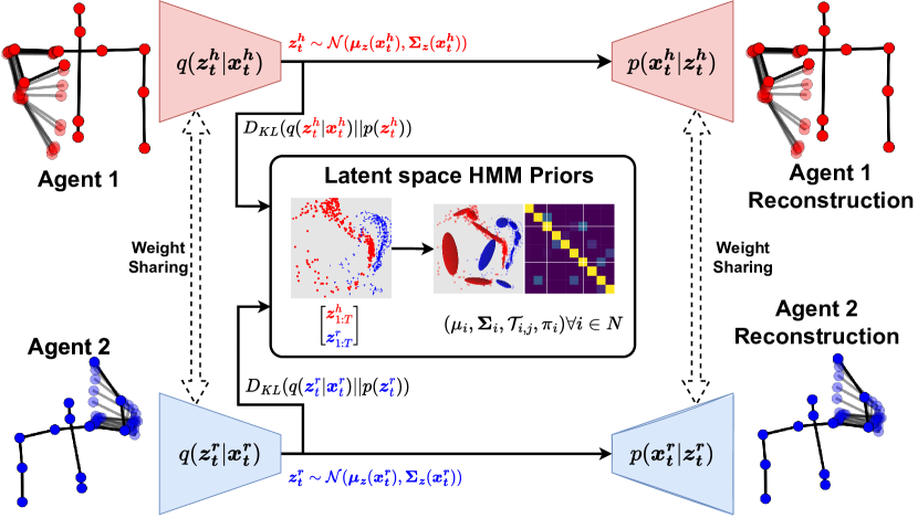
(a) Learning Interaction Models from Human-Human Interactions.

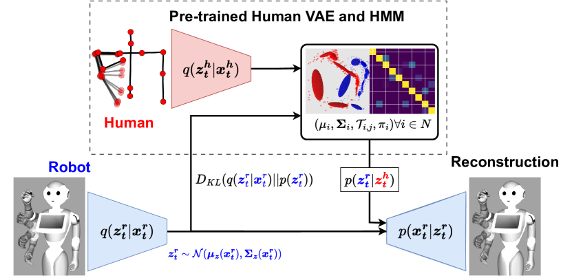
(b) Using Human-Human Interaction models for Human-Robot Interaction models.

Figure 3: Overview of our training approach. We model the interaction dynamics in the latent space of a VAE using HMMs to model a joint distribution over the latent trajectories of both agents. The use of HMMs for the prior, as opposed to a unimodal Gaussian, enforces a multimodal modularized latent space with the HMM forward variable incorporating the learned transitions between the multiple modes. We first learn the interaction dynamics from Human-Human demonstrations by training both the VAEs and HMMs (Figure 3(a)). We subsequently use the HMM prior learned from Human-Human demonstrations for learning the latent dynamics for HRI. We do so by regularizing the robot VAEs and additionally, by training the robot decoder to reconstruct samples from the HMM’s conditional distribution after observing the human partner (Figure 3(b)). This further incorporates the interdependence between the human and the robot during training thereby improving the predicted robot trajectories.

In this section, we introduce our overall approach which can be seen in Figure 3. We start by explaining the key idea of our previous work MILD [65] which enhances the representation learning abilities of VAEs with HMMs as the prior distribution for modeling the interaction dynamics (Section III-A). After introducing our previous work, we go through the key improvements on top of MILD, namely incorporating the human-conditioned HMM distribution for reactive motion generation into the training process in Section III-B followed by the adaptation of the learned trajectories via Inverse Kinematics for improving the generated robot motions as well as the incorporation of stiffness control in Section III-C. For HRI scenarios, we use the superscripts $h$ and $r$ to denote the human and the robot variables respectively. For consistency, in the HHI scenarios, we use $h$ and $r$ to denote the variables of the first and second human partners respectively.

III-A Learning Interaction Dynamics using HMMs as VAE priors

Typically in VAEs, the prior $p(\boldsymbol{z})$ is modeled as a stationary distribution. When it comes to learning trajectory dynamics, having meaningful priors can help learn temporally coherent latent spaces [22]. To this end, we explore the use of HMMs to learn latent-space dynamics in a modular manner by breaking down the trajectories into multiple phases and learning the sequencing between them. Since the HMMs learn a joint distribution over the latent trajectories of both interacting agents, we can conditionally generate the motion of the robot after observing the human agent. We do so by using the HMM distribution as the prior for the VAE. We then update the HMM at the end of each epoch by running expectation-maximization on the VAE embeddings, alternating between training the VAE and then subsequently updating the HMM.

The VAE prior at each time-step is calculated as the respective marginal distribution of the most likely HMM component at that timestep, given by the HMM forward variable (Eq. 4). However, the recurrent nature of estimating the forward variable, and consequently its gradients, leads to numerical instabilities from backpropagation through time. Hence, we use an approximation in the form of an unobserved forward variable by setting the likelihood term in Eq. 4 to unity. This unobserved forward variable provides a good approximation of the sequential progression of the hidden states based on the learned transitions which can be written as

$$\begin{gathered}\bar{\alpha}_{i}^{t}=\frac{\hat{\alpha}_{i}^{t}}{\sum_{j=1}^{N}\hat{\alpha}_{j}^{t}}\hskip 10.00002pt\hat{\alpha}_{i}^{t}=\sum_{j=1}^{N}\bar{\alpha}_{j}^{t-1}\mathcal{T}_{j,i}\hskip 10.00002pt\hat{\alpha}_{i}^{0}=\pi_{i}\\ i^{*}_{t}=\operatorname*{arg\,max}_{i}\bar{\alpha}_{i}^{t}\\ KL_{t}^{h}=KL(q(\boldsymbol{z}^{h}_{t}|\boldsymbol{x}^{h}_{t})||\mathcal{N}(\boldsymbol{z}^{h}_{t};\boldsymbol{\mu}^{h}_{i^{*}_{t}},\boldsymbol{\Sigma}^{hh}_{i^{*}_{t}}))\\ KL_{t}^{r}=KL(q(\boldsymbol{z}^{r}_{t}|\boldsymbol{x}^{r}_{t})||\mathcal{N}(\boldsymbol{z}^{r}_{t};\boldsymbol{\mu}^{r}_{i^{*}_{t}},\boldsymbol{\Sigma}^{rr}_{i^{*}_{t}}))\end{gathered}$$ (14)

where $\mathcal{N}(\boldsymbol{z}^{h}_{t};\boldsymbol{\mu}^{h}_{i^{*}_{t}},\boldsymbol{\Sigma}^{hh}_{i^{*}_{t}}))$ and $\mathcal{N}(\boldsymbol{z}^{r}_{t};\boldsymbol{\mu}^{r}_{i^{*}_{t}},\boldsymbol{\Sigma}^{rr}_{i^{*}_{t}})$ are the marginal distributions of the most likely HMM component $i^{*}_{t}$ at the given timestep $t$ for each agent. The ELBO can then be reformulated as

$$\mathbb{E}_{q}[\log\frac{p(\boldsymbol{x}^{h}_{t},\boldsymbol{x}^{r}_{t},\boldsymbol{z}^{h}_{t},\boldsymbol{z}^{r}_{t})}{q(\boldsymbol{z}^{h}_{t},\boldsymbol{z}^{r}_{t}|\boldsymbol{x}^{h}_{t},\boldsymbol{x}^{r}_{t})}] =\mathbb{E}_{q}[\log p(\boldsymbol{x}^{h}_{t}|\boldsymbol{z}^{h}_{t})]$$ (15)

$$+\mathbb{E}_{q}[\log p(\boldsymbol{x}^{r}_{t}|\boldsymbol{z}^{r}_{t})]$$

$$-\beta(KL_{t}^{h}+KL_{t}^{r}).$$

The overall training procedure, shown in Algorithm 1 and Figure 3(a), is as follows. We train the VAE to reconstruct the input trajectory and use the marginal distributions of each agent from the HMM (Eq. 14) to regularize the latent posterior distribution. During a given epoch in the VAE training, the HMM parameters are fixed. After an epoch, the new HMM parameters are estimated using the learned encodings $\boldsymbol{z}^{h}_{1:T},\boldsymbol{z}^{r}_{1:T}$ of the training trajectories. The HMMs are then fixed as the VAE prior for the next epoch. Currently, we learn a separate HMM per interaction. We defer learning the HMM selection via activity recognition to future work. For further details on training HMMs with expectation-maximization, or the use of HMMs in robot learning, we refer the reader to [26, 14].

Data: A set of trajectories with action labels $\boldsymbol{X}=\{\boldsymbol{X}^{h}_{1:T},\boldsymbol{X}^{r}_{1:T},c\}$ for $|\mathcal{C}|$ interactions

Result: VAE weights and $|\mathcal{C}|$ HMM parameters

Initialize VAE weights randomly

for $c\in[1,|\mathcal{C}|]$ do

       for $i\in[1,N]$ do

             $\boldsymbol{\mu}^{c}_{i}\leftarrow\boldsymbol{0}$

             $\boldsymbol{\Sigma}^{c}_{i}\leftarrow\boldsymbol{I}$

            

       end for

      

end for

while not converged do

       for $\boldsymbol{x}^{h}_{1:T},\boldsymbol{x}^{r}_{1:T},c\in\boldsymbol{X}$ do

             Compute VAE Posterior $q(\boldsymbol{z}^{h}_{t}|\boldsymbol{x}^{h}_{t})$ and $q(\boldsymbol{z}^{r}_{t}|\boldsymbol{x}^{r}_{t})$

             Reconstruct posterior samples

             Maximize ELBO (Eq. 15) to update VAE weights

            

       end for

      for $c\in[1,|\mathcal{C}|]$ do

             $\boldsymbol{X}^{c}\leftarrow$ set of demonstrations of Interaction $c$

             $\boldsymbol{Z}^{c}\leftarrow\emptyset$

             for $\boldsymbol{x}^{h}_{1:T},\boldsymbol{x}^{r}_{1:T},c\in\boldsymbol{X}^{c}$ do

                   $\boldsymbol{z}^{h}_{1:T}\sim q(\cdot|\boldsymbol{x}^{h}_{1:T});\boldsymbol{z}^{r}_{1:T}\sim q(\cdot|\boldsymbol{x}^{r}_{1:T})$

                   $\boldsymbol{Z}^{c}\leftarrow\boldsymbol{Z}^{c}\cup\begin{bmatrix}\boldsymbol{z}^{h}_{1:T}\\ \boldsymbol{z}^{r}_{1:T}\end{bmatrix}$

                  

             end for

            Train the $c^{th}$ HMM with $\boldsymbol{Z}^{c}$

       end for

      

end while

Algorithm 1 Learning Latent Dynamics from Human-Human Interactions

III-B Conditional Training of HRI Dynamics from HHI

Based on the initial idea of [65] presented above in Section III-A, in this section, we first explore how the HMMs learned from the Human-Human demonstrations can be used to regularize learning the robot motions, after which we highlight the incorporation of the conditional generation of the robot motions. The HMMs learned from Human-Human demonstrations capture the overall latent interaction dynamics between two agents. These HMMs can therefore be used as an informative prior for learning robot motions to perform the given interaction. Hence, we use the marginal distribution of the second agent from the HMMs trained on the HHI demonstrations as the latent space prior for the robot VAE. Although we regularize the VAEs with the HMM marginals (Eq. 14), during test time the decoder would see samples from the conditional distribution of the HMM after observing the human agent (Eq. 6-11) which would be finitely divergent from what the decoder would be trained to reconstruct in a normal autoencoding approach.

When the output spaces of both interaction partners are similar, such as in the HHI scenarios sharing the weights of the VAEs for can enable the decoder to learn to reconstruct the target distribution. However, given the difference in output spaces of the human and the robot in HRI scenarios, we instead train the robot decoder to additionally reconstruct samples from conditional distribution (Figure 3(b)).

Moreover, the VAE provides a confidence estimate of the posterior probability which can additionally be incorporated into the conditional distribution $p(\boldsymbol{z}_{t}^{r}|\boldsymbol{z}_{t}^{h})$ as

$$\boldsymbol{K}_{i} ={\color[rgb]{1,.5,0}\boldsymbol{\Sigma}^{rh}_{i}}({\color[rgb]{1,.5,0}\boldsymbol{\Sigma}^{hh}_{i}}+{\color[rgb]{1,0,1}\boldsymbol{\Sigma}_{\boldsymbol{z}}(\boldsymbol{x}^{h}_{t})})^{-1}$$ (16)

$$\boldsymbol{\hat{\mu}}^{r}_{i} ={\color[rgb]{1,.5,0}\boldsymbol{\mu}^{r}_{i}}+\boldsymbol{K}_{i}({\color[rgb]{1,0,1}\boldsymbol{\mu}_{\boldsymbol{z}}(\boldsymbol{x}^{h}_{t})}-{\color[rgb]{1,.5,0}\boldsymbol{\mu}^{h}_{i}})$$ (17)

$$\boldsymbol{\hat{\Sigma}}^{r}_{i} ={\color[rgb]{1,.5,0}\boldsymbol{\Sigma}^{rr}_{i}}-\boldsymbol{K}_{i}{\color[rgb]{1,.5,0}\boldsymbol{\Sigma}^{hr}_{i}}+\boldsymbol{\hat{\mu}}^{r}_{i}(\boldsymbol{\hat{\mu}}^{r}_{i})^{T}$$ (18)

$$\boldsymbol{\hat{\mu}}^{r}_{t} =\sum_{i=1}^{N}{\color[rgb]{1,.5,0}\bar{\alpha}_{i}^{t}}\hskip 1.99997pt\boldsymbol{\hat{\mu}}^{r}_{i}$$ (19)

$$\boldsymbol{\hat{\Sigma}}^{r}_{t} =\left[\sum_{i=1}^{N}{\color[rgb]{1,.5,0}\bar{\alpha}_{i}^{t}}\hskip 1.99997pt\boldsymbol{\hat{\Sigma}}^{r}_{i}\right]-\boldsymbol{\hat{\mu}}^{r}_{t}(\boldsymbol{\hat{\mu}}^{r}_{t})^{T}$$ (20)

$$p(\boldsymbol{z}_{t}^{r}|{\color[rgb]{1,0,1}q_{t}^{h}}) =\mathcal{N}(\boldsymbol{z}^{r}_{t};\boldsymbol{\hat{\mu}}^{r}_{t},\boldsymbol{\hat{\Sigma}}^{r}_{t})$$ (21)

where the terms in magenta are from the human VAE posterior $q_{h}^{t}=q(\boldsymbol{z}^{h}_{t}|\boldsymbol{x}^{h}_{t})$ and the terms in orange are from the HMM. We then reconstruct samples from $p(\boldsymbol{z}_{t}^{r}|{\color[rgb]{1,0,1}q_{t}^{h}})$ thereby allowing the robot VAE’s decoder to be trained with samples drawn from a distribution similar to what it would encounter during test time, instead of just using samples from the posterior. Our modified ELBO at each timestep for training the robot VAE in the HRI scenario (Algorithm 2) can be written as

$$\mathbb{E}_{q}[\log\frac{p(\boldsymbol{x}^{h}_{t},\boldsymbol{x}^{r}_{t},\boldsymbol{z}^{r}_{t})}{q(\boldsymbol{z}^{r}_{t}|\boldsymbol{x}^{h}_{t},\boldsymbol{x}^{r}_{t})}] =\mathbb{E}_{q_{r}}\log p(\boldsymbol{x}^{r}_{t}|\boldsymbol{z}^{r}_{t})$$ (22)

$$-\beta KL_{t}^{r}$$

$$+\mathbb{E}_{\boldsymbol{z}^{r}_{t}\sim p(\boldsymbol{z}^{r}_{t}|q^{h}_{t})}\log p(\boldsymbol{x}^{r}_{t}|\boldsymbol{z}^{r}_{t})$$

where the first term is the reconstruction term, $KL_{t}^{r}$ is the regularization term calculated according to Eq. 14, and the third term denotes the reconstruction of the conditional samples drawn from $p(\boldsymbol{z}^{r}_{t}|q_{t}^{h})$ (Eq. 21). Both the reconstruction term and the conditional reconstruction are estimated in a Monte Carlo fashion by averaging the loss over multiple samples drawn from the corresponding latent distributions.

Data: A set of trajectories with action labels $\boldsymbol{X}=\{\boldsymbol{X}^{h}_{1:T},\boldsymbol{X}^{r}_{1:T},c\}$ for $|\mathcal{C}|$ actions, Human VAE and HMMs

Result: Robot VAE weights

Initialize VAE weights randomly

while not converged do

       for $\boldsymbol{x}^{h}_{1:T},\boldsymbol{x}^{r}_{1:T},c\in\boldsymbol{X}$ do

             Compute VAE Posterior $q(\boldsymbol{z}^{r}_{t}|\boldsymbol{x}^{r}_{t})$

             Compute Latent Conditional $p(\boldsymbol{z}_{t}^{r}|q_{t}^{h})$ (Eq. 16-21)

             Reconstruct posterior and conditional samples

             Maximize ELBO (Eq. 22) to update VAE weights

            

       end for

      

end while

Algorithm 2 Learning HRI Dynamics

During testing, we first encode the observations of the human agent $\boldsymbol{x}^{h}_{t}$ and then condition the HMM $p(\boldsymbol{z}_{t}^{r}|q_{t}^{h})$ to generate the latent trajectory of the second agent $\hat{\boldsymbol{z}}^{r}_{t}$ using Eq. 16 - 21, which is then decoded to obtain the actions of the second agent $p(\hat{\boldsymbol{x}}^{r}_{t}|\boldsymbol{z}^{r}_{t})$.

III-C Inverse Kinematics Adaptation and Stiffness Modulation

In typical LfD approaches, robot motions are learned via kinesthetic teaching [62, 71]. In HRI scenarios, kinesthetic teaching gives good results [28, 5, 16, 13] but can become tedious when trying to generalize to multiple human interaction partners. One way to circumvent this could be to execute randomized open-loop trajectories for the robot and learn how the human adapts to the robot motions [17].

Since we are dealing with a Humanoid robot, we learn the robot motions using the kinematic similarities between the human and the robot [31]. From the 3D positions of an arm, we extract the shoulder angles (yaw, pitch, and roll) and the bending of the elbow by using the geometry of the tracked skeleton, as seen in Figure 4. We defer the calculation of the wrist angle to our future work and instead use a fixed value for the wrist for each interaction.

Since we extract joint angles from the human demonstrations, some inaccuracies are present due to slight differences between the kinematic structure of the human skeleton and the robot. Given the difference in the arm dimensions of the Pepper robot and a human, the spatial accuracy of the learned behaviors is quite limited. Additionally, given the smaller size of the Pepper robot, its reachability is also limited, thereby limiting the ability to learn task space trajectories.

To bridge the mismatch in motion retargeting, we adapt the predicted motions during test time with Inverse Kinematics to reach the human partner’s hand while using the predicted motions as a prior. The use of Inverse Kinematics enables the physical proximity needed by the interaction while keeping the robot configuration close to the demonstrated behaviors [33]. Moreover, we do not need to use Inverse Kinematics all the time, but only in the segments involved in physical contact. We therefore inspect the underlying segments of the HMM manually to see which segments comprise of the contact-based portion of the trajectory and which ones do not, and subsequently perform the IK adaptation only in the contact-based segments.

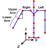
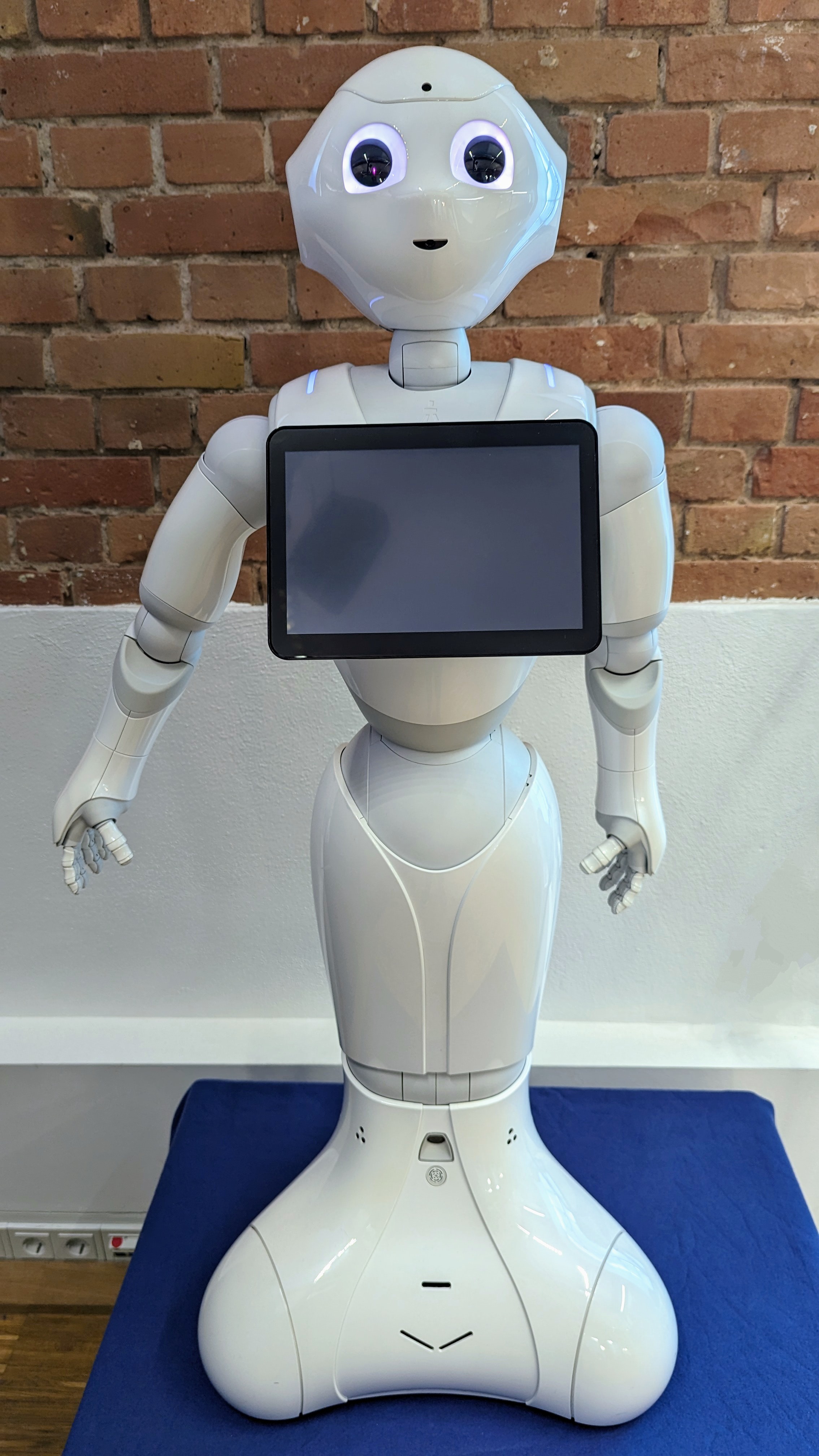
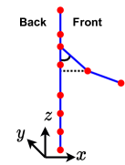
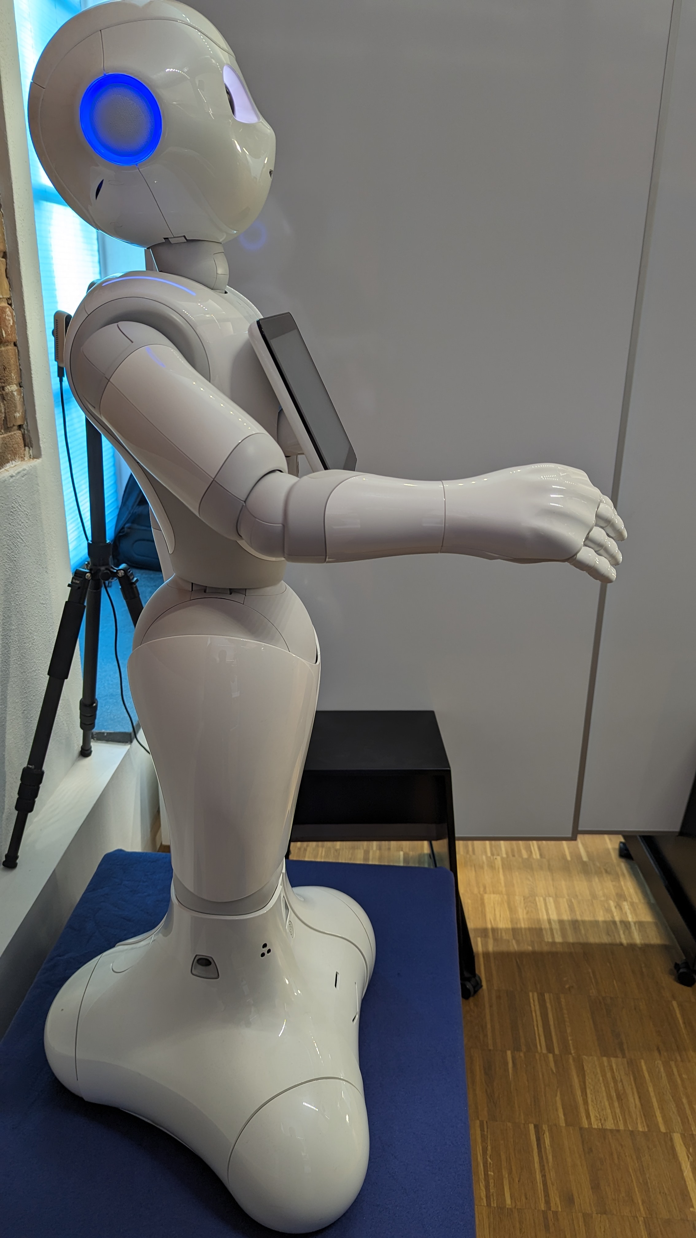
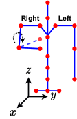
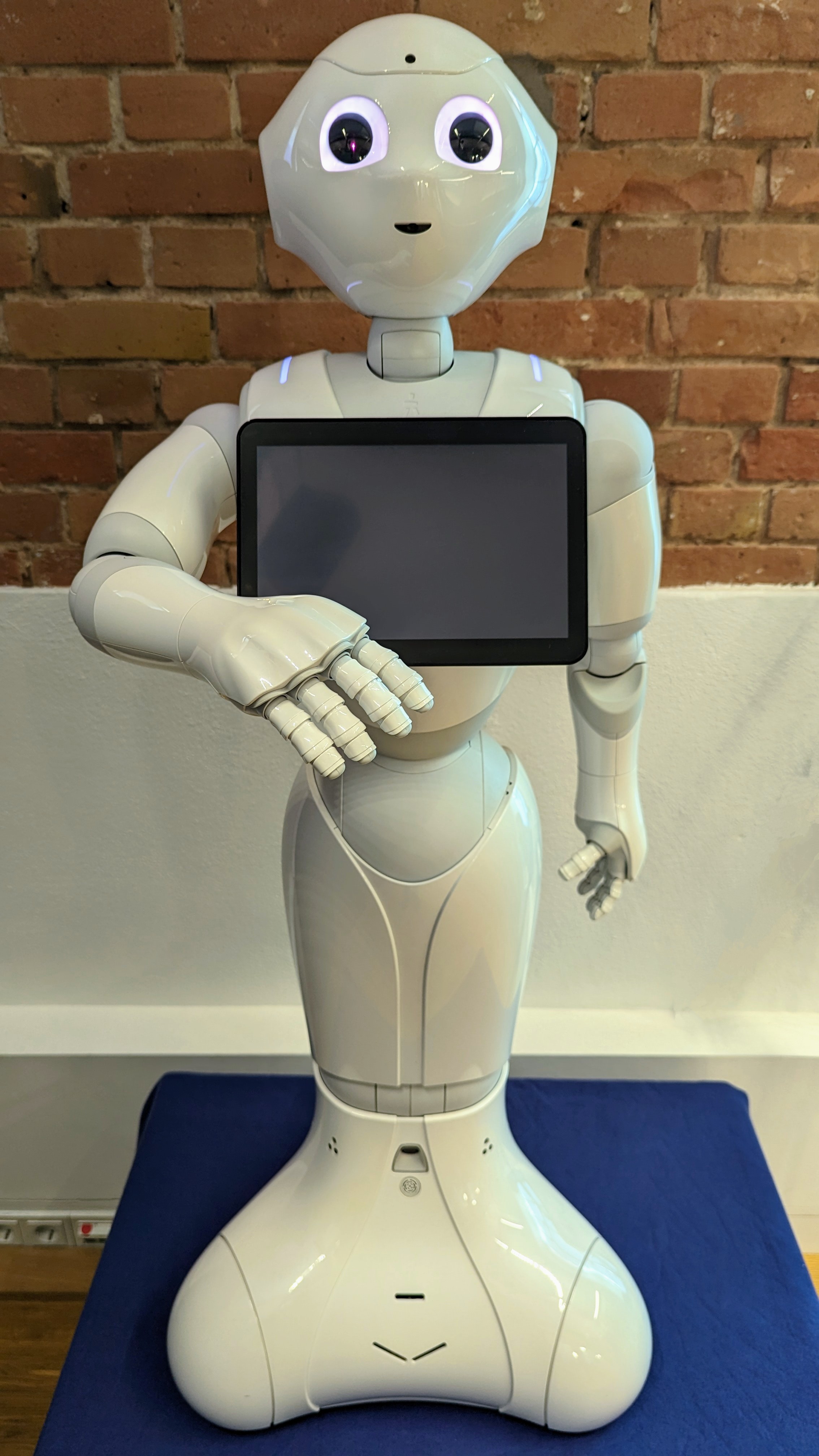
Figure 4: Geometric similarities between the degrees of freedom of a human’s upper body and the humanoid robot Pepper. The shoulder roll, pitch, yaw, and elbow angle of a human can be directly mapped to Pepper’s joint angles.

Given an initial prediction of the robot’s joint angle distribution $(\boldsymbol{\mu}_{\boldsymbol{q}},\boldsymbol{\Sigma}_{\boldsymbol{q}})$ and a task space goal in 3D space $(\boldsymbol{\mu}_{\boldsymbol{x}},\boldsymbol{\Sigma}_{\boldsymbol{x}})$ (which in this case is the human partner’s hand position), we aim to find a joint angle configuration $\boldsymbol{q}^{*}$ that reaches $\boldsymbol{\mu}_{\boldsymbol{x}}$, but does not stray too far from $\boldsymbol{\mu}_{\boldsymbol{q}}$ [33] which boils down to the following optimization problem

$$\begin{split}\boldsymbol{q}^{*}=\operatorname*{\arg\max}_{\boldsymbol{q}}\mathcal{N}&(f(\boldsymbol{q})|\boldsymbol{\mu}_{\boldsymbol{x}},\boldsymbol{\Sigma}_{\boldsymbol{x}})\mathcal{N}(\boldsymbol{q}|\boldsymbol{\mu}_{\boldsymbol{q}},\boldsymbol{\Sigma}_{\boldsymbol{q}})\\ =\operatorname*{\arg\min}_{\boldsymbol{q}}\lambda_{\boldsymbol{x}}&(\boldsymbol{\mu}_{\boldsymbol{x}}-f(\boldsymbol{q}))^{T}\boldsymbol{\Sigma}_{\boldsymbol{x}}^{-1}(\boldsymbol{\mu}_{\boldsymbol{x}}-f(\boldsymbol{q}))+\\ \lambda_{\boldsymbol{q}}&(\boldsymbol{\mu}_{\boldsymbol{q}}-\boldsymbol{q})^{T}\boldsymbol{\Sigma}_{\boldsymbol{q}}^{-1}(\boldsymbol{\mu}_{\boldsymbol{q}}-\boldsymbol{q})\end{split}$$ (23)

where $f(\boldsymbol{q})$ is the forward kinematics model of the robot to estimate the end-effector location given the joint angles $\boldsymbol{q}$, and $\lambda_{\boldsymbol{x}},\lambda_{\boldsymbol{q}}$ are relative weights balancing whether it is more important to stay close to the initial distribution or to reach the task space goal. In practice, $\boldsymbol{\mu}_{\boldsymbol{q}}$ comes from the VAE decoder $p(\boldsymbol{x}^{r}_{t}|\boldsymbol{z}^{r}_{t})$, $\boldsymbol{\mu}_{\boldsymbol{x}}$ comes from the human observation $\boldsymbol{x}^{h}_{t}$ and we set $\boldsymbol{\Sigma}_{\boldsymbol{q}}$ and $\boldsymbol{\Sigma}_{\boldsymbol{x}}$ to identity. We can then simplify Eq. 23 to

$$\boldsymbol{q}^{*}=\operatorname*{\arg\min}_{\boldsymbol{q}}\lambda_{\boldsymbol{x}}\lVert\boldsymbol{\mu}_{\boldsymbol{x}}-f(\boldsymbol{q})\rVert^{2}+\lambda_{\boldsymbol{q}}\lVert\boldsymbol{\mu}_{\boldsymbol{q}}-\boldsymbol{q}\rVert^{2}$$ (24)

where $\lVert\cdot\rVert$ denotes the Euclidean norm.

Moreover, we do not need to employ IK during every segment of the interaction. Once the training converges, we identify the segments from the underlying HMM that correspond to the contact-based phases of the interaction. Based on the HMM’s forward variable prediction from the human observation, we adapt the human-conditioned robot motions using IK if the current segment is contact-based. The incorporation of IK is further detailed in Algorithm 3.

Data: An observation of the human agent $\boldsymbol{x}^{h}_{1:t}$, trained VAE and HMM Models, a set of contact-based HMM states $\mathcal{I}$ for the given interaction

Result: Conditioned Trajectory for the second agent $\hat{\boldsymbol{x}}^{r}_{1:t}$

for $t\in[1,T]$ do

       Encode the human observation $q(\boldsymbol{z}^{h}_{t}|\boldsymbol{x}^{h}_{t})$

       Compute Latent Conditional $p(\boldsymbol{z}_{t}^{r}|q_{t}^{h})$ (Eq. 16-21)

       Decode the conditioned prediction $\boldsymbol{\mu}_{\boldsymbol{q}}=p(\hat{\boldsymbol{x}}^{r}_{t}|\hat{\boldsymbol{z}}^{r}_{t})$

       if $\operatorname*{\arg\max}_{i}\alpha_{i}(\boldsymbol{z}^{h}_{t})$ is a contact-based segment then

             $\hat{\boldsymbol{q}}_{t}=\operatorname*{\arg\min}_{\boldsymbol{q}}\lambda_{\boldsymbol{x}}\lVert\boldsymbol{\mu}_{\boldsymbol{x}}-f(\hat{\boldsymbol{q}}_{t})\rVert^{2}+\lambda_{\boldsymbol{q}}\lVert\boldsymbol{\mu}_{\boldsymbol{q}}-\boldsymbol{q}\rVert^{2}$

      else

            $\hat{\boldsymbol{q}}_{t}=\boldsymbol{\mu}_{\boldsymbol{q}}$

       end if

      Send $\hat{\boldsymbol{q}}_{t}$ to the robot controller.

end for

Algorithm 3 Conditioning on Human Observations and IK Adaptation

In a contact-rich interaction like handshaking, along with moving in a coordinated manner, the robot must be compliant with the human’s motion when in contact. When executing handshaking trajectories on the robot, we use the forward variable not just for calculating the target pose of the robot, but also to detect when to lower the target joint stiffness once the robot enters the contact-based segments of the interaction.

During a handshaking interaction with the robot, to prevent sudden changes in stiffness arising from the misclassification of the segment, we disable back-transitions into the initial reaching segment. Additionally, since the forward variable is calculated using only the human partner’s latent state during test time, we found some mismatches in the segment prediction compared to using the full joint human-robot states for timesteps near the transition boundary between the initial reaching segment and the subsequent segments. Therefore, taking a leaf out of Transition State Clustering [43], we learn an additional distribution over the states that get misclassified at the transition boundary between the reaching and contact phase. We use this additional transition state distribution to detect when the interaction proceeds into the contact-based segments when the probability of either the contact segment or the transition state exceeds that of the reaching segment. Doing so gives a better indication of when to lower the robot’s stiffness and provides a more suitable interaction. Without such a scheme, due to the misclassification of the active segment, the joint stiffness would not always be lowered correctly, thereby resulting in a rigid and non-compliant handshake.

IV Experiments and Results

In this section, we first provide our implementation details (Section IV-A) and the datasets used (Section IV-B). We then present the results of predicting the controlled agent’s trajectories after conditioning on the observed agent in Section IV-C and finally, we discuss our user-study in Section IV-D.

IV-A Experimental Setup

The VAEs are implemented using PyTorch [63] with 2 hidden layers in the encoder and decoder each with sizes (40, 20) and (20, 40) respectively and a 5-dimensional latent space with Leaky ReLU activations [48] at all layers except the output layer. The weights are initialized using Xavier’s initialization [32]. The networks are trained with $\beta~{}=~{}5\times 10^{-3}$, 10 Monte Carlo samples per input data and using the Adam optimizer with weight decay [47] with a learning rate of $5\times 10^{-4}$. In the HHI scenarios, we share the parameters of the VAEs for both human agents as the inputs are structurally similar. The networks were trained for 400 epochs. The best out of 4 seeds were used to report the results.

A separate HMM is trained for each interaction. The HMMs are implemented using a custom PyTorch version of PbDLib [64]. Each HMM has 6 hidden states, which we found as the most numerically stable. The HMMs are initialized by splitting each of the latent trajectories in the training set into equally sized segments over time. To prevent numerical instabilities arising from vanishing values in the HMM covariance matrices, we add a small positive regularization constant of $10^{-4}$ to the diagonal elements. When sampling from the conditional distribution, due to numerical errors in computing the Cholesky decomposition of the covariance matrices, rather than adding a constant value to all elements, we add linearly increasing regularization based on the dimensions, going from $9.1\times 10^{-5}$ for the first dimension to $10^{-4}$ for the last dimension. Additionally, we adapt the covariance matrices of the conditional distribution by iteratively adding an even smaller constant that is proportional to the absolute value of the smallest eigenvalue of the covariance matrix to the diagonal elements [36].

We implement our approach on the Pepper robot [60], which is a 1.2m tall humanoid robot that has the same degrees of freedom in its arm as a human. For Inverse Kinematics, we use the IKPy library [51] which uses the least squares minimization in SciPy [83] for the IK optimization. We set $\lambda_{\boldsymbol{x}}=1$ and $\lambda_{\boldsymbol{q}}=0.01$ for the objective function in Eq. 24.

IV-B Dataset

IV-B1 Bütepage et al. [13]

record HHI and HRI demonstrations of 4 interactions: Waving, Handshaking, and two kinds of fist bumps. The first fistbump called “Rocket Fistbump”, involves bumping fists at a low level and then raising them upwards while maintaining contact with each other. The second is called “Parachute Fistbump” in which partners bump their fists at a high level and bring them down while simultaneously oscillating the hands sideways, while in contact with each other. Since our testing scenario involves the humanoid robot Pepper [60], we additionally extract the joint angles from one of the human partner’s skeletons from the above-mentioned HHI data for the Pepper robot using the similarities in DoFs between a human and Pepper [31, 66] (Figure 4), which we denote this as “HRI-Pepper”. Bütepage et al. [13] additionally record demonstrations of these actions with a human partner interacting with an ABB YuMi-IRB 14000 robot controlled via kinesthetic teaching. We call this scenario as “HRI-Yumi”.

In the HHI scenario (and the HRI-Pepper scenario), there are 181 trajectories (32 - Waving, 38 - Handshake, 70 - Rocket Fistbump, 49 - Parachute Fistbump) of which 80% of the trajectories (149 trajectories) are used for training and the rest (32 trajectories) for testing. In the HRI-Yumi scenario, there are 41 trajectories (10 each for Waving, Handshaking, and Rocket Fistbump and 11 for Parachute Fistbump) of which we use a similar split with 32 trajectories for training and 9 for testing. We use a time window of 5 observations as the input for a given timestep as done in [13]. We downsample the data to 20Hz to match our testing scenario.

We use the 3D positions and the velocities (represented as position deltas) of the right arm joints (shoulder, elbow, and wrist), with the origin at the shoulder, leading to an input size of 90 dimensions (5x3x6: 5 timesteps, 3 joints, 6 dimensions) for a human partner. For the HRI-Pepper and HRI-Yumi scenarios, we use a similar window of joint angles, leading to an input size of 20 dimensions (5x4) for the 4 joint angles of Pepper’s right arm and an input size of 35 dimensions (5x7) for the 7 joint angles of Yumi’s right arm.

IV-B2 Nuitrack Skeleton Interaction Dataset

(NuiSI) is a dataset which we collected ourselves of the same 4 interactions as in [13], namely Waving, Handshaking, Rocket Fistbump and Parachute Fistbump. The skeleton data of two human partners interacting with one another is recorded using two Intel Realsense D435 cameras (one recording each human partner). We use Nuitrack [1] for tracking the upper body skeleton joints in each frame at 30Hz. As done above with [13], we additionally extract the joint trajectories for the Pepper robot, which leaves us finally with both the HHI and HRI-Pepper scenarios. We have 44 trajectories (12 - Waving, 11 - Handshaking, 12 - Rocket Fistbump, 9 - Parachute Fistbump) of which we similarly use 80% of the trajectories for training (33 trajectories) and the rest (11 trajectories) for testing.

The skeletons are then rotated such that they follow the orientation shown in Figure 4 with the $x$-axis in the forward direction, the $y$-axis going from right to left, and the $z$-axis in the upward direction. For training, the data is processed similarly as mentioned above with a window size of 5 time steps. Given the relatively low amount of samples, we finetune the network trained on the aforementioned dataset of [13]. As done with [13], we extract the joint angles for the Pepper robot from the skeleton trajectories for the HRI-Pepper scenario [31, 66].

IV-C Conditioned Prediction Results

We test the conditioning ability of our approach compared to [13] to evaluate the accuracy of the generated motions of the controlled agent after observing the human interaction-partner. We evaluate the approaches over the four interactions of the dataset in [13] and our collected data (NuiSI). We calculate the Mean Squared Error (MSE) averaged over each joint and the 5-time step window.

TABLE I: Prediction MSE (in cm) for the second human partner’s trajectories after observing the first human partner averaged over all joints and timesteps. (* – $p<0.05$, ** – $p<0.01$, lower is better)

Dataset	Action	MILD v1	[13]
[13]	Hand Wave	0.788 $\pm$ 1.226∗∗	4.121 $\pm$ 2.252
	Handshake	1.654 $\pm$ 1.549∗	1.181 $\pm$ 0.859
	Rocket Fistbump	0.370 $\pm$ 0.682	0.544 $\pm$ 1.249
	Parachute Fistbump	0.537 $\pm$ 0.579∗∗	0.977 $\pm$ 1.141
NuiSI	Hand Wave	0.408 $\pm$ 0.538∗∗	3.168 $\pm$ 3.392
	Handshake	0.311 $\pm$ 0.259∗∗	1.489 $\pm$ 3.327
	Rocket Fistbump	1.142 $\pm$ 1.375∗∗	3.576 $\pm$ 3.082
	Parachute Fistbump	0.453 $\pm$ 0.578∗∗	2.008 $\pm$ 2.024

TABLE II: Prediction MSE (in radians) for robot trajectories after observing the human interaction partner averaged over all joints and timesteps. (Lower is better, lowest values highlighted in bold, significance shown in Table A.1)

Dataset	Action	MILD v1	MILD v2.1	MILD v2.2	MILD v3.1	MILD v3.2	Bütepage et al. [13]
HRI-Yumi [13]	Hand Wave	1.705 $\pm$ 0.521	1.349 $\pm$ 1.972	1.641 $\pm$ 1.968	1.033 $\pm$ 1.204	1.143 $\pm$ 1.330	0.225 $\pm$ 0.302
	Handshake	0.290 $\pm$ 0.148	0.073 $\pm$ 0.040	0.068 $\pm$ 0.052	0.104 $\pm$ 0.056	0.123 $\pm$ 0.069	0.133 $\pm$ 0.214
	Rocket Fistbump	0.428 $\pm$ 0.175	0.236 $\pm$ 0.167	0.183 $\pm$ 0.122	0.130 $\pm$ 0.074	0.128 $\pm$ 0.071	0.147 $\pm$ 0.119
	Parachute Fistbump	0.425 $\pm$ 0.150	0.028 $\pm$ 0.042	0.033 $\pm$ 0.034	0.028 $\pm$ 0.034	0.028 $\pm$ 0.035	0.181 $\pm$ 0.155
HRI-Pepper [13]	Hand Wave	0.267 $\pm$ 0.152	0.161 $\pm$ 0.228	0.165 $\pm$ 0.189	0.103 $\pm$ 0.103	0.106 $\pm$ 0.105	0.664 $\pm$ 0.277
	Handshake	0.327 $\pm$ 0.253	0.111 $\pm$ 0.092	0.153 $\pm$ 0.154	0.061 $\pm$ 0.048	0.056 $\pm$ 0.041	0.184 $\pm$ 0.141
	Rocket Fistbump	0.161 $\pm$ 0.095	0.035 $\pm$ 0.068	0.035 $\pm$ 0.068	0.021 $\pm$ 0.037	0.018 $\pm$ 0.035	0.033 $\pm$ 0.045
	Parachute Fistbump	0.265 $\pm$ 0.178	0.116 $\pm$ 0.176	0.112 $\pm$ 0.181	0.095 $\pm$ 0.151	0.088 $\pm$ 0.148	0.189 $\pm$ 0.196
HRI-Pepper (NuiSI)	Hand Wave	0.760 $\pm$ 0.325	0.050 $\pm$ 0.084	0.060 $\pm$ 0.087	0.046 $\pm$ 0.059	0.049 $\pm$ 0.059	0.057 $\pm$ 0.093
	Handshake	0.225 $\pm$ 0.114	0.025 $\pm$ 0.022	0.025 $\pm$ 0.020	0.021 $\pm$ 0.015	0.020 $\pm$ 0.014	0.083 $\pm$ 0.075
	Rocket Fistbump	0.354 $\pm$ 0.238	0.077 $\pm$ 0.095	0.080 $\pm$ 0.088	0.077 $\pm$ 0.067	0.079 $\pm$ 0.072	0.101 $\pm$ 0.086
	Parachute Fistbump	0.201 $\pm$ 0.072	0.032 $\pm$ 0.038	0.028 $\pm$ 0.040	0.025 $\pm$ 0.028	0.022 $\pm$ 0.027	0.049 $\pm$ 0.040

We do not train with the conditional loss in the Human-Human scenarios since we use shared weights, the decoder already learns to reconstruct the ground truth samples for the conditional distribution. Additionally, we found that the interplay between the shared weights and the conditional training discussed in Section III-B would cause the HMM posterior to collapse into a single unimodal distribution. Therefore, we only show comparisons of our vanilla approach presented in Section III-A, which we denote as “MILD v1”.

The results of MILD v1 in predicting the interaction partner’s trajectories in the HHI scenarios can be seen in Table I. It can be seen that MILD v1 with its simplistic nature of using an HMM for the latent dynamics performs significantly better (as verified with a Mann-Whitney U Test) than [13] where the VAEs are trained with an uninformative standard normal distribution as a prior. Although additional LSTMs are employed in [13] to learn the latent dynamics, since the VAEs are trained with an uninformative prior, their approach fails to accurately reconstruct motions the learnt latent dynamics. In contrast, the latent dynamics of each segment of the interaction is captured well by the HMM which therefore acts as an informative prior for the VAEs which is reflected in the improved prediction accuracy of MILD v1.

Coming to HRI scenarios, starting from the initial incorporation of the HMM prior as shown in Section III-A (denoted as “MILD v1”), we explore two variants of $\mathcal{L}_{cond}^{t}$ in Eq. 22. The first is with reconstructing the conditional latent predictions (i.e. the mean in Eq. 19) of samples drawn from the posterior distribution both with and without the use of the VAE posterior covariance (in Eq. 16). This can be summarized mathematically as $\mathbb{E}_{q(\boldsymbol{z}^{h}_{t}|\boldsymbol{x}^{h}_{t})}\log p(\boldsymbol{x}^{r}_{t}|\boldsymbol{\mu}^{r}_{t})$ where $\boldsymbol{\mu}^{r}_{t}$ is calculated using Eq. 9 with samples drawn from $q(\boldsymbol{z}^{h}_{t}|\boldsymbol{x}^{h}_{t})$. We explore this variant both without and with the posterior covariance in Eq. 16, denoted as “MILD v2.1” and “MILD v2.2” respectively

The second variant uses the posterior mean and covariance to calculate the conditional distribution and subsequently reconstruct samples drawn from the conditional distribution. This can be summarized mathematically as $\mathbb{E}_{p(\boldsymbol{z}^{r}_{t}|q^{h}_{t})}\log p(\boldsymbol{x}^{r}_{t}|\boldsymbol{z}^{r}_{t})$ where $p(\boldsymbol{z}^{r}_{t}|q^{h}_{t})$ is calculated using Eq. 16 - 21 and the samples drawn from this distribution are reconstructed. We explore this variant both without and with the posterior covariance in Eq. 16, which we denote as “MILD v3.1” and “MILD v3.2” respectively. The differences between the different variants are summarized in Table III.

TABLE III: Differences in conditioning and sampling strategies of the variants of MILD.

Variant	Conditional Training Inputs	Samples given to Decoder
MILD v1	None	Only Posterior Samples
MILD v2.1	Posterior Samples	Posterior Samples and their corresponding conditioned outputs
1-2 MILD v2.2	Posterior Samples and Covariance
MILD v3.1	Posterior Mean	Posterior Samples, Conditional Samples
1-2 MILD v3.2	Posterior Mean and Covariance

As seen in Table II, reconstructing samples from the conditional distribution (MILD v3.1 and v3.2) provides much better results as compared to conditioning samples drawn from the posterior (MILD v2.1 and v2.2), both of which perform better than MILD v1 that does not use conditional training. The samples drawn from the conditional distribution would be more representative of the type of samples that the decoder would see during run time. While in theory, enough samples from the posterior, when conditioned, can also estimate this distribution, empirically, this fails to match up to sampling from the conditional distribution. One argument for this is that reconstructing conditional samples enables learning a joint latent space more susceptible to the HMM conditioning.

Furthermore, the overall improvement in performance compared to MILD v1 and [13] highlights the advantage of incorporating the conditional distribution into the training process for reactive motion generation. The importance of incorporating reactive motion generation into the training can also be seen in the improved performance of [13] over MILD v1 in the HRI scenarios as compared to the HHI scenarios.This improvement comes from the fact that MILD uses the HMMs just as a latent prior, whereas in [13], the authors explicitly train a separate HRI dynamics model for predicting the robot motions from the latent trajectories of both the human and the robot. During testing however, the HRI dynamics network does not have access to the ground truth target of the robot which is used to train the network. Therefore, the HRI dynamics is predicted in an autoregressive manner, which deteriorates the performance due to out-of-distribution data. In this regard, it can be seen that explicitly incorporating such conditional out-of-distribution samples can lead to better results, as seen in the improved performance of the variants of MILD (v2.1 - v3.2).

Some examples of the learned behaviors, along with the progression of the HMM in the latent space can be seen in Figure 6, where we show a sample interaction for handshake (Figure 6(a)) and rocket fistbump (Figure 6(b)) on the Pepper robot. As it can be seen, the HMM captures the sequencing between the multiple modes of the latent space to generate suitable motions for real-world HRI scenarios. This is additionally validated via a user study (Section IV-D) which shows the ability of our approach to generalize well to various users, despite being trained on demonstrations of just two partners.

IV-D HRI User Study

To see the effectiveness of our approach in producing acceptable physical behaviors, we conducted a user study where participants interacted with the robot. We evaluate our proposed approach both with and without IK adaptation, denoted as “MILD-IK” and “MILD” (while we use “MILD v3.2”, for ease of notation, we shorten it to “MILD”) against a baseline IK algorithm (Eq. 13) that uses the human’s hand pose as the target location (“Base-IK”). We run this study for two interactions, handshake and rocket fistbump. The study design was given a positive vote by the Ethics Commission at TU Darmstadt (Application EK 48/2023).

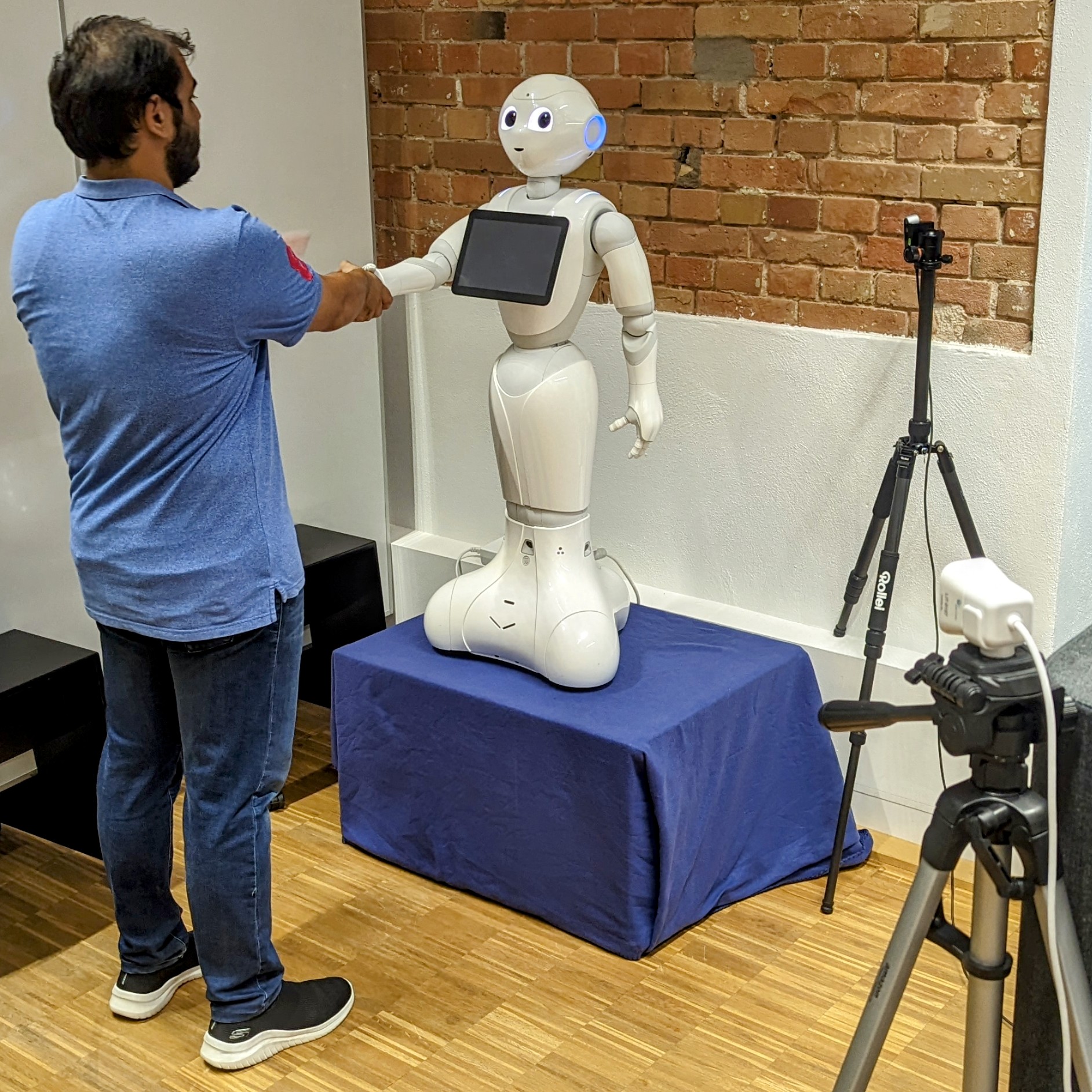
Figure 5: Setup of the User Study for interacting with the Pepper robot. As Pepper is quite short (1.2m), it is placed on a pedestal to match the height of a human partner. The camera behind Pepper tracks the human partner’s motion, which is used to generate Pepper’s motions.

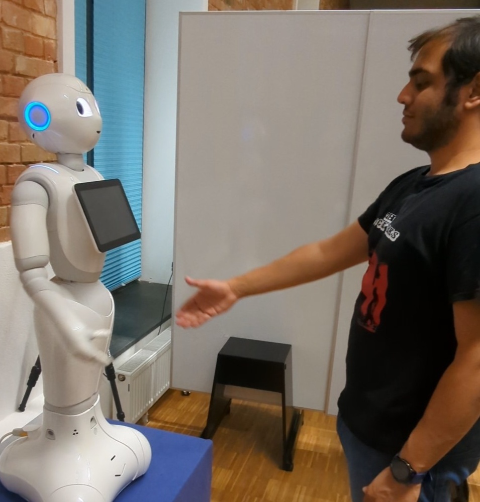
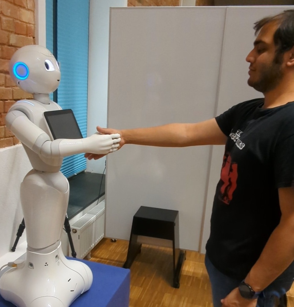
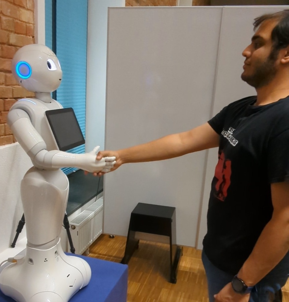
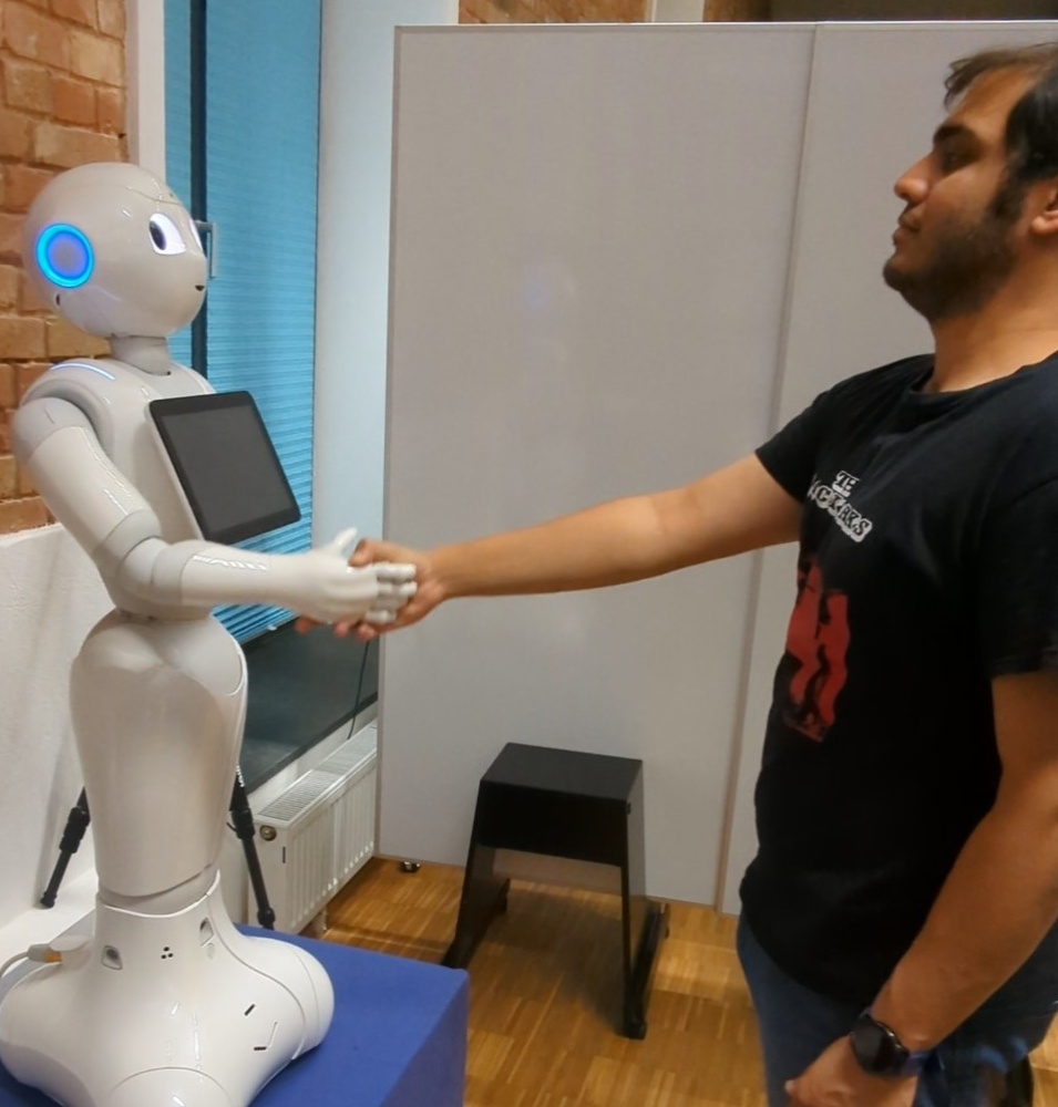
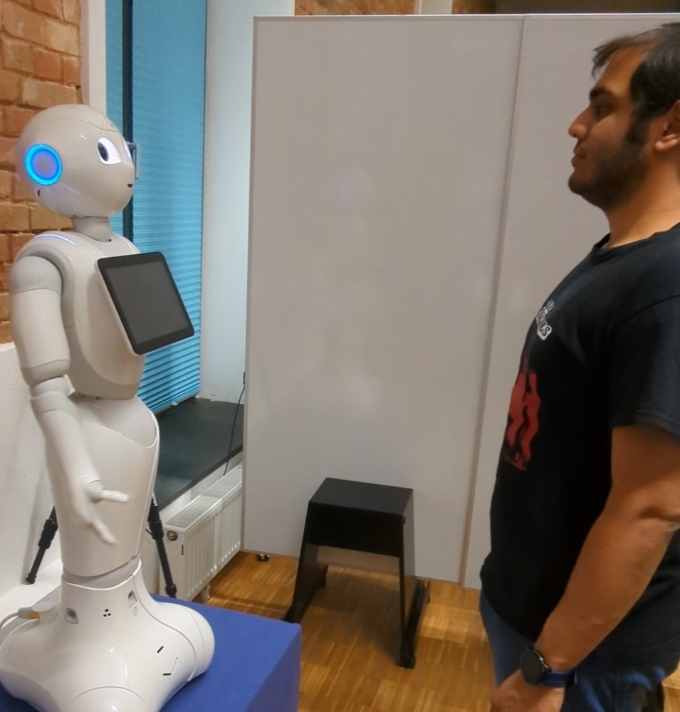
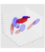
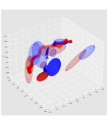
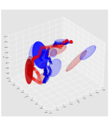
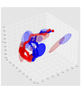
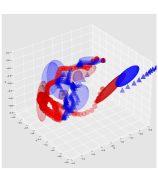
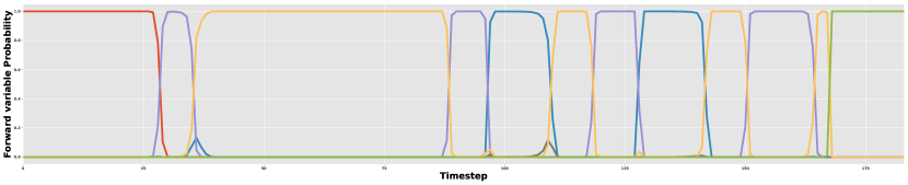
(a) Sample Handshake HRI

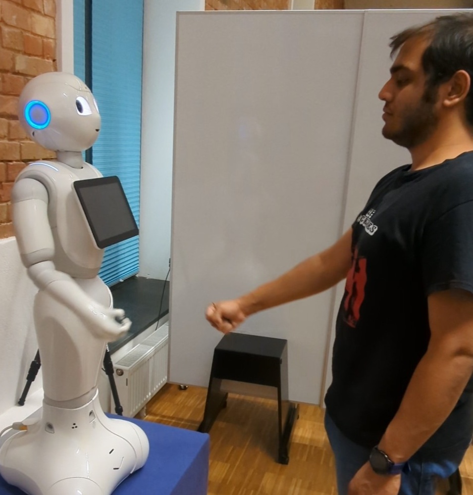
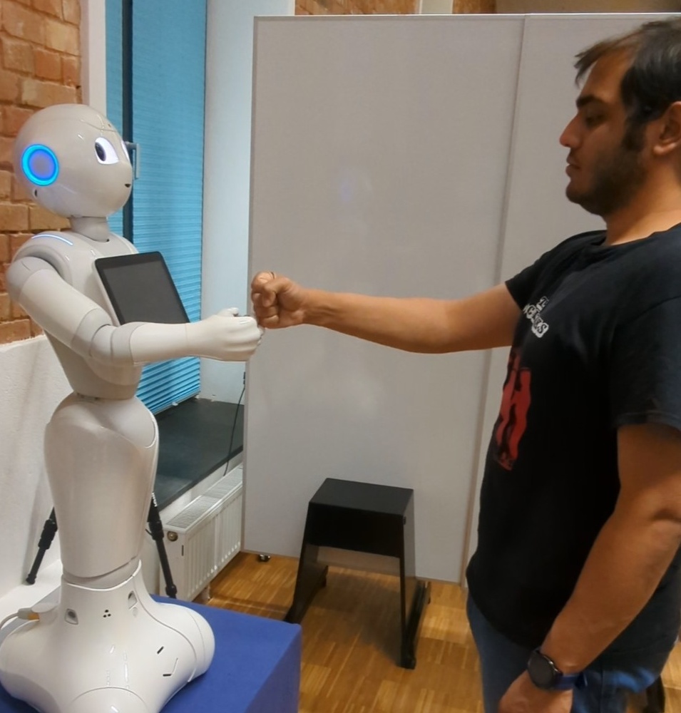
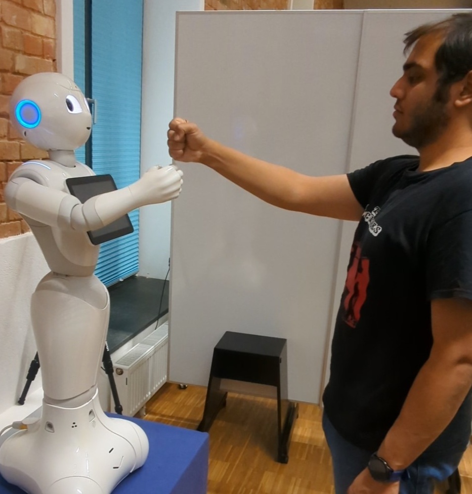
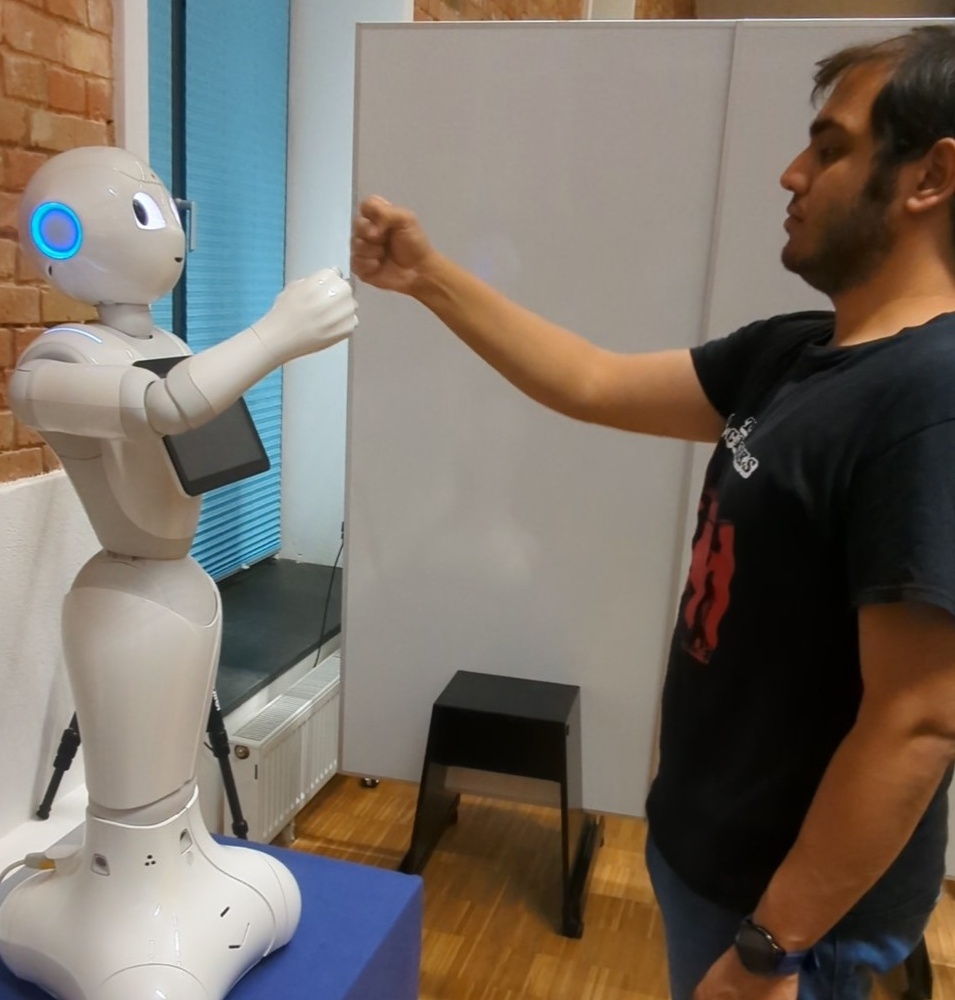
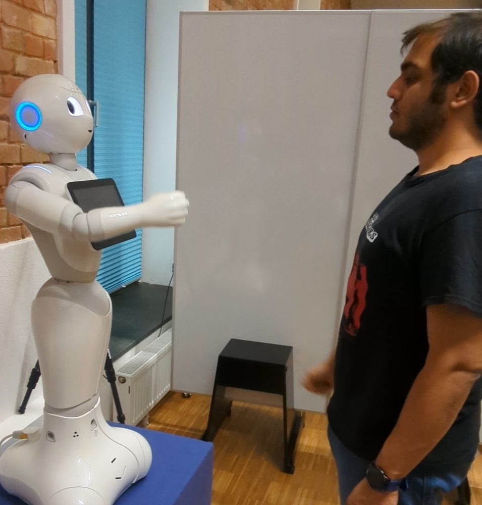
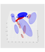
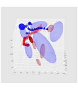
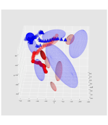
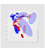
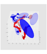
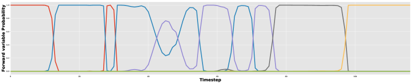
(b) Sample Rocket HRI

Figure 6: Sample sequences for the Handshake and Rocket fistbump interactions on the Pepper robot. The top row of each interaction shows the result of the generated reactive motion after observing the human partner’s skeleton. The middle row shows the latent trajectories and the HMM segments over the first 3 dimensions of the latent space (Red - Human, Blue - Robot). The opacity of each cluster is the corresponding cluster probability, given by the HMM forward variable. The progression of the HMM forward variable is shown in the bottom row, with different colors denoting the different segments.

IV-D1 Procedure

The study took place in a laboratory setting (Figure 5) where participants were initially guided to a desk to fill out a consent form followed by a pre-questionnaire which included demographic information, prior experiences with robots, their attitude towards robots [79], attitude towards physical interactions, and some personality questions to gauge extroversion [67]. We assessed these measures to gain additional information about our sample. Participants were then shown an instruction video of two humans performing an interaction (either a handshake or a rocket fistbump). Participants were then given the experiment protocol to read wherein they were instructed that they had to lead the interaction with the robot. Additionally, some general instructions were provided regarding the limits of the robot and how they should position themselves.

Participants were then guided behind a barrier where they would see the robot for the first time and would then stand at an adequate distance from the robot. When they were ready, an initial interaction was performed with a hard-coded motion. This is to get the participant habituated to the way the robot moves and counter any novelty effects that may occur and to have the participant better understand how to perform the interaction with the robot. After the initial run, the participant was informed that the experimental trials would begin. The sequence of each trial was as follows:

1. Before each trial, the participant would see a video stream of the skeleton tracker to better position themselves.

2. Once the position was set and the tracking was stable, the experimenter would signal them to start the trial.

3. The participant would start the interaction and the robot would respond reactively.

4. Once the participant goes back to a neutral position with their hands by their side, the robot arm would go back to a neutral position, marking the end of the trial.

5. This process would then repeat once again after which the participant was asked to fill out a questionnaire.

This process constitutes a single session and was repeated 3 times (3 sessions in total) wherein the robot was controlled by one of the three aforementioned algorithms (Base-IK, MILD, MILD-IK). The algorithms were shown in randomized order to all participants to avoid sequence effects. The participant was neither informed of the randomization nor the algorithm they were interacting with. After all 3 sessions, the participant was asked to fill out a final questionnaire where they had to rank the sessions based on their preference and answer some open-ended questions about the sessions.

IV-D2 Participant Sample

A total of 20 users (8 female, 12 male) participated in our study and were recruited through the university environment. Of the 20 participants, 10 performed the Rocket fistbump (4 female, 6 male) and the rest performed a handshake. The mean age of the participants was 27.85 years (SD: 3.51). Participants had an average level of experience with robots overall on a scale from 1 (no experience at all) to 5 (a lot of experience) with a mean of 2.90 (SD: 1.45). They had quite a positive attitude towards robots on a scale from 1 (very negative) to 7 (very positive) with a mean of 5.90 (SD: 1.16). This is also consistent with the ratings regarding the attitudes towards robots for the following items on a scale of 1 (Strongly Agree) to 7 (Strongly Disagree). Participants largely had a high agreement towards feeling relaxed when interacting with robots (Mean: 5.60, SD: 1.05) and high levels of disagreement towards being paranoid when interacting with a robot (Mean: 1.85, SD: 0.93) and towards feeling nervous standing in front of a robot (Mean: 1.80, SD:1 .06). Participants had a positive outlook towards physical interactions in general on a scale from 1 (distant) to 7 (open) with a mean of 6.10 (SD: 0.84). This was also confirmed with the Big 5 extroversion scale [67] with a mean extroversion of 4.75 (SD: 1.34) out of 7.

IV-D3 Methodology

The study followed a within-subject design where participants interacted with a Pepper robot controlled by each of the aforementioned algorithms twice in a randomized order, leading to 6 HRIs per participant. Each participant had to either perform a handshake or a fistbump, not both. We do so as the focus of our paper is on understanding how our proposed algorithm is perceived by users, therefore we do not focus on the differences between the interaction types. We break the 6 trials into 3 sessions, where each session corresponds to two trials of a given algorithm. Each session was evaluated with 16 different items adapted from the Godspeed [7] and the SASSI [38] questionnaires, each rated on a 5-Point scale (1 - Strongly disagree, 5 - Strongly agree):

• The interaction with the robot was pleasant.

• The interaction with the robot was exciting.

• The interaction with the robot was human-like.

• The interaction with the robot was natural.

• The interaction with the robot was friendly.

• The interaction with the robot was comfortable.

• The interaction with the robot was well-timed.

• The interaction with the robot was accurate.

• The interaction with the robot was annoying.

• The interaction with the robot was awkward.

• The interaction with the robot was scary.

• The robot interacted in an aggressive way.

• I am satisfied with the way the robot interacted with me.

• The second trial in the session was more effortless than the first.

At the end of the experiment, we asked the participants to rank the 3 sessions (algorithms) in their order of preference.

We run a one-way Repeated Measures ANOVA to compare the responses of the different algorithms followed by paired sample t-tests for a post hoc analysis (Table IV).

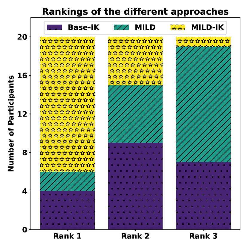
Figure 7: Participant’s ranking of the algorithms. (MILD-IK - yellow stars, MILD - green lines, Base-IK - purple dots). Most participants ranked MILD-IK first, better than both Base-IK and MILD.

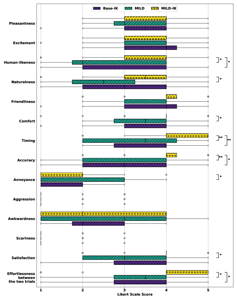
Figure 8: Boxplot of the comparison between the three different approaches. (* - $p<0.05$, ** - $p<0.01$)

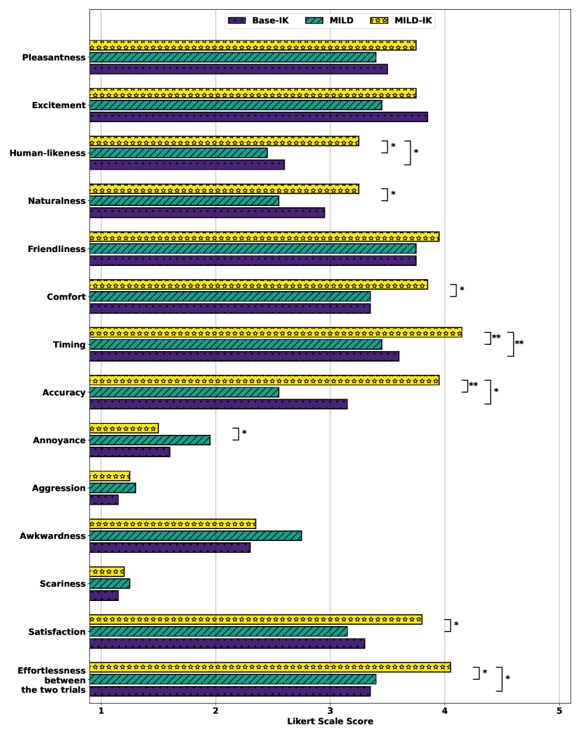
Figure 9: Barplot of the comparison between the three different approaches. (* - $p<0.05$, ** - $p<0.01$)

Base-IK	MILD	MILD-IK

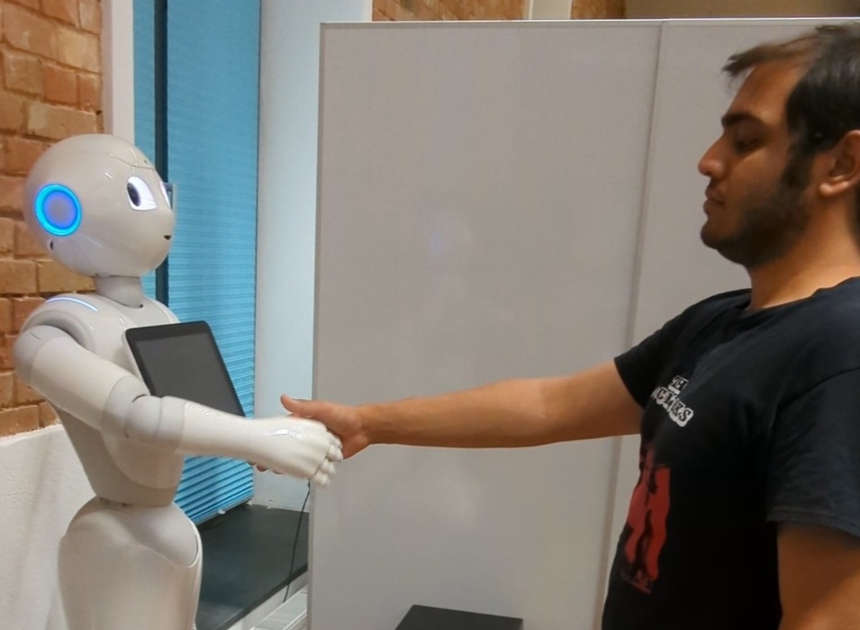
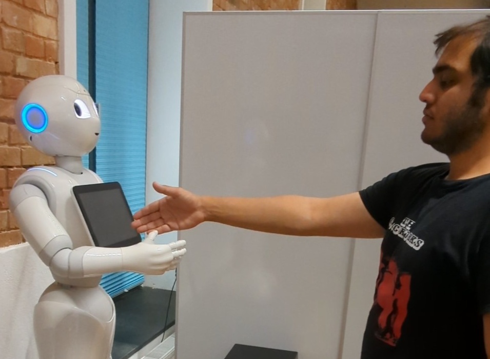
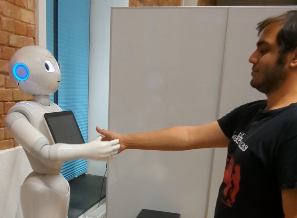
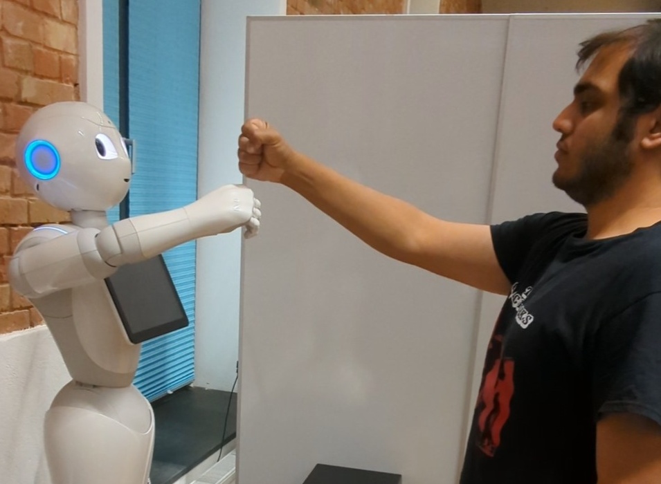
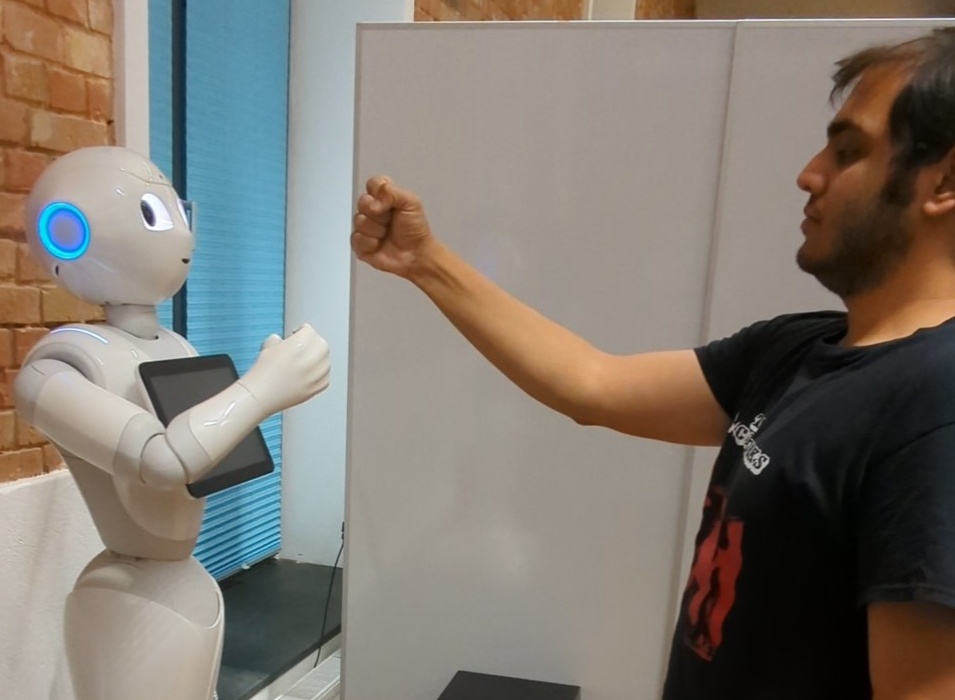
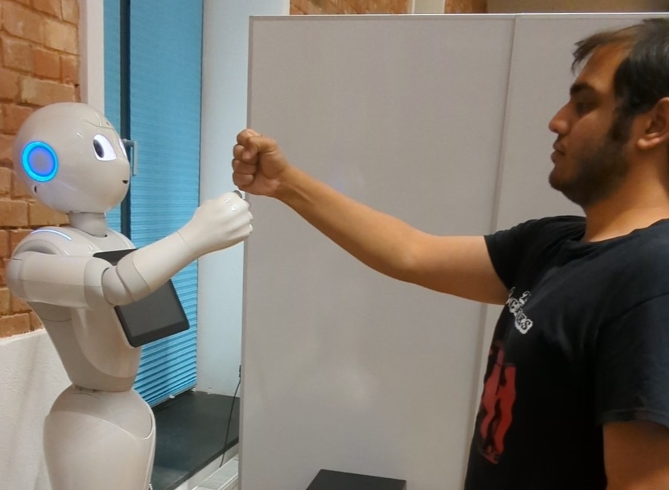
Figure 10: Peculiarities of the different algorithms. The “Base-IK” approach reaches the human’s hand but awkwardly with the robot hand rotated inwards and the elbow pointing out. MILD maintains a human-like posture but falls short of reaching the partner’s hand due to the mismatch in motion retargeting. However, MILD-IK accurately reaches the human’s hand while maintaining a human-like posture.

IV-D4 Study Results

As seen in Figure 7, MILD-IK was by far ranked in the first place much more than MILD which was by far the least ranked, and Base-IK which was mostly ranked second. Just using MILD without IK was the least preferred among the algorithms, even though it was programmed keeping the interactiveness in mind, but due to the motion retargeting issues mentioned in Section III-C, it is unable to reach the participant’s hand accurately, leading to a low acceptance by the participants which can further be seen in the results in Figures 8 and 9.

All approaches have similarly high levels of pleasantness, excitement, and friendliness and similarly low levels of annoyance, aggression, and scariness. This goes to show that the overall interaction scenario was well perceived by the participants and can additionally be attributed to an overall positive attitude toward robots.

TABLE IV: Results of a one-way Repeated Measures ANOVA for each of the survey items. Values less than 0.01 are reported as 0. The last three columns show the mean differences between the different algorithms (1 - Base-IK, 2 - MILD, 3 - MILD-IK) which were analyzed using paired sample t-tests (* - $p<0.05$, ** - $p<0.01$).

Survey Item Anova Results Base-IK MILD MILD-IK $\Delta\mu_{1,2}$ $\Delta\mu_{3,2}$ $\Delta\mu_{3,1}$ Survey Item $F_{2,38}$ $p$-value Mean SD Mean SD Mean SD Pleasantness 0.86 0.43 3.50 1.07 3.40 1.07 3.75 0.89 0.10 0.35 0.25 Excitement 1.32 0.28 3.85 0.85 3.45 1.02 3.75 0.89 0.40 0.30 -0.10 Human-likeness 4.89 0.01 2.60 1.20 2.45 1.16 3.25 1.22 0.15 0.80* 0.65* Naturalness 3.46 0.04 2.95 1.24 2.55 1.20 3.25 1.18 0.40 0.70* 0.30 Friendliness 0.56 0.58 3.75 1.04 3.75 0.83 3.95 0.86 0.00 0.20 0.20 Comfort 2.79 0.07 3.35 1.06 3.35 0.96 3.85 0.96 0.00 0.50* 0.50 Timing 5.77 0.01 3.60 1.07 3.45 1.16 4.15 0.96 0.15 0.70** 0.55* Accuracy 10.15 0.00 3.15 1.28 2.55 1.24 3.95 0.86 0.60 1.40 0.80 Annoyance 2.08 0.14 1.60 0.80 1.95 1.20 1.50 0.81 -0.35 -0.45* -0.10 Aggression 0.77 0.47 1.15 0.48 1.30 0.64 1.25 0.62 -0.15 -0.05 0.10 Awkwardness 2.29 0.12 2.30 1.05 2.75 1.34 2.35 1.24 -0.45 -0.40 0.05 Scariness 0.59 0.56 1.15 0.48 1.25 0.54 1.20 0.51 -0.10 -0.05 0.05 Satisfaction 2.54 0.09 3.30 1.14 3.15 0.96 3.80 0.87 0.15 0.65* 0.50 Effortlessness between the two trials 4.15 0.02 3.35 1.19 3.40 1.16 4.05 1.24 -0.05 0.65* 0.70*

Since the Base-IK approach does not have any prior over the IK solutions, it would lead to poses where the elbow is pointed outwards and the hand is turned sideways, which participants remarked was unnatural and awkward. Even though it was able to reach the human’s hand location, this unnatural pose of the robot hand prevented the Base-IK approach from being able to reach the human hand in a graspable manner, due to the orientation of the end-effector. This is also reflected via a significantly lower accuracy rating for Base-IK and can further be seen in relatively lower (although non-significant) trends for naturalness, comfort, and satisfaction.

Participants found MILD awkward at times since the predicted motions would sometimes fall short of the partner’s hand and the robot would thereby not reach the participants’ hand correctly. This can especially be seen in the low accuracy that is given to MILD. This reachability issue gets mitigated with MILD-IK as it generates more natural poses. However, with MILD-IK, since the prediction of when to start the IK adaptation comes from the HMM, there would be a distinct moment when the robot hand would reach the human’s hand, which we attribute as a possible reason for a relatively higher awkwardness rating.

Overall, the high acceptability of MILD-IK is also reflected via significantly better ratings of the human-likeness, timing, and perceived accuracy. The effortlessness between two trials in an interaction was also rated significantly higher for MILD-IK showing that it was easier for participants to get habituated to the movements of the robot. MILD-IK also achieves a higher rating for timing, which is attributed to the ability of the HMM to generate the receding motion in a reactive manner, unlike Base-IK which would still try to reach the hand until the participant would go back to a neutral pose. Some of these peculiarities can be seen in Figure 10.

V Conclusion and Future Work

In this paper, we proposed a system for learning real-world HRI from demonstrations of Human-Human Interactions (HHI). We first learned latent interaction dynamics from the HHI demonstrations in a modular manner using Hidden Markov Models (HMMs) and then demonstrated how the learned dynamics were utilized for learning HRI behaviors. We further showed how the learning of HRI behaviors was improved by incorporating the conditional distribution of the HMM into the training process. This enabled more accurate reactive motion generation during test time which we found is an important aspect of achieving a competitive performance. We then demonstrated the adaptation of the reactively generated robot trajectories during test time with Inverse Kinematics, thereby successfully combining the spatial accuracy of task-space adaptation with the ease of learning joint-space trajectories in a manner that improved the exactness of the learned behaviors. For a contact-rich task like handshaking, we additionally showed how the HMM segment predictions can be used for stiffness modulation to improve the overall perceived quality of the interaction. Through a user study, we found that our method is better perceived by human users in terms of human-likeness, timing, accuracy, and effortlessness. Our user study further validates the effectiveness of our approach in generalizing well to multiple users despite being trained on data from just two interaction partners.

V-A Limitations

While the current approach generated acceptable and accurate response trajectories that, there are still some limitations to our approach which we highlight below. Currently, while training the VAE and HMM together as in the HHI scenario with the conditional loss as in the HRI scenario, we frequently encountered mode collapse of the HMM hidden states. This is why we resort to freezing the learned HMM and Human VAE for training on the HRI scenarios. This could stem from a bad approximation of the forward variable that does not accurately capture the progression of the hidden states but would rather favor just a few or a single state, thereby exacerbating the mode collapse. While this might be solved by propagating gradients through the forward variable, we found that this brings numerical issues arising from the recurrent nature of the forward variable computation, which leads to vanishing/exploding gradients (as in typical RNNs). Mitigating this issue would enable one to incorporate the HMMs into the training process in a more mathematically sound manner.

Although we train the HMMs jointly over the latent spaces of both interacting agents, during testing, we use only the human observations.This can lead to inaccuracies in predicting the state of the interaction when solely using human observations as compared to the joint set of observations of both agents (as highlighted in the appendix). Incorporating the current state of the robot and the relative geometry between the human and the robot into the training process could improve the overall predictive performance of the network.

V-B Future Work

On the practical side, coming to the interaction with the robot, we purposely left out auxiliary behaviors such as speech or gaze that make the robot more “alive” as our focus was to evaluate the different interaction algorithms. These auxiliary behaviors could help improve the overall perceived quality of the interaction. The influence of the inherent personality traits also affects the interaction [19]. Further research into quantifying such influences, for example, based on the mental states of the human partner [2] or with underlying emotions [4, 78], to adapt the robot actions and personalize the interactions leading can subsequently provide a more natural interaction and improve the perception of the robot. Additionally, for handshaking, exploring more traditional stiffness and impedance control for the Pepper robot to improve its compliance [12, 11] can help improve the interaction.

From the learning side, the current bottleneck of our approach both in terms of training times and in achieving accurate predictions is the HMM. Currently, we train the HMMs independently from the VAE in a separate step. In this regard, one could look at incorporating this into the variational framework in a more principled manner [6] or training the HMMs and VAEs in a more closely coupled manner by propagating the gradients of the expectation-maximization through the VAE could yield more suitable representations for the task at hand. Alternatively, we plan to look at going beyond HMMs by using neural variants for incorporating the multimodality such as Mixture Density Networks [9] with larger encoder backbones to additionally handle visual inputs, which are important for functional HRI tasks in settings involving shared autonomy with a human, such as object handovers or collaborative manipulation. Additionally, incorporating a GAN-like discriminator [85] or diffusion-based architectures [56] could lead to performance improvements over a VAE, especially for more diverse tasks.

TABLE A.1: $p$-values for pairwise MSE comparisons of the results reported in Table II. For $p<0.001$, we report zeros.

			Version of MILD
			v1	v2.1	v2.2	v3.1	v3.2
HRI-Yumi [13]	Waving	[13]	0.	0.	0.	0.	0.
		MILD v1	–	0.	0.	0.	0.
		MILD v2.1	–	–	0.	0.284	0.337
		MILD v2.2	–	–	–	0.	0.
		MILD v3.1	–	–	–	–	0.675
	Handshake	[13]	0.	0.	0.397	0.	0.
		MILD v1	–	0.	0.	0.	0.
		MILD v2.1	–	–	0.018	0.	0.
		MILD v2.2	–	–	–	0.	0.
		MILD v3.1	–	–	–	–	0.008
	Rocket Fistbump	[13]	0.	0.	0.	0.976	0.999
		MILD v1	–	0.	0.	0.	0.
		MILD v2.1	–	–	0.	0.	0.
		MILD v2.2	–	–	–	0.	0.
		MILD v3.1	–	–	–	–	0.909
	Parachute Fistbump	[13]	0.	0.136	0.098	0.	0.
		MILD v1	–	0.	0.	0.055	0.
		MILD v2.1	–	–	0.785	0.	0.
		MILD v2.2	–	–	–	0.	0.
		MILD v3.1	–	–	–	–	0.003
HRI-Pepper [13]	Waving	[13]	0.	0.	0.	0.	0.
		MILD v1	–	0.	0.	0.	0.
		MILD v2.1	–	–	0.	0.	0.
		MILD v2.2	–	–	–	0.	0.
		MILD v3.1	–	–	–	–	0.119
	Handshake	[13]	0.	0.	0.	0.	0.
		MILD v1	–	0.	0.	0.	0.
		MILD v2.1	–	–	0.	0.	0.
		MILD v2.2	–	–	–	0.	0.
		MILD v3.1	–	–	–	–	0.041
	Rocket Fistbump	[13]	0.	0.291	0.838	0.	0.
		MILD v1	–	0.	0.	0.	0.
		MILD v2.1	–	–	0.	0.	0.
		MILD v2.2	–	–	–	0.	0.
		MILD v3.1	–	–	–	–	0.
	Parachute Fistbump	[13]	0.	0.	0.	0.	0.
		MILD v1	–	0.	0.	0.	0.
		MILD v2.1	–	–	0.016	0.	0.
		MILD v2.2	–	–	–	0.	0.
		MILD v3.1	–	–	–	–	0.018
HRI-Pepper (Nuisi)	Waving	[13]	0.	0.	0.139	0.158	0.309
		MILD v1	–	0.	0.	0.	0.
		MILD v2.1	–	–	0.	0.	0.
		MILD v2.2	–	–	–	0.004	0.530
		MILD v3.1	–	–	–	–	0.014
	Handshake	[13]	0.	0.	0.	0.	0.
		MILD v1	–	0.	0.	0.	0.
		MILD v2.1	–	–	0.862	0.095	0.003
		MILD v2.2	–	–	–	0.104	0.007
		MILD v3.1	–	–	–	–	0.065
	Rocket Fistbump	[13]	0.	0.	0.	0.	0.
		MILD v1	–	0.	0.	0.	0.
		MILD v2.1	–	–	0.036	0.	0.
		MILD v2.2	–	–	–	0.050	0.023
		MILD v3.1	–	–	–	–	0.685
	Parachute Fistbump	[13]	0.	0.	0.	0.	0.
		MILD v1	–	0.	0.	0.	0.
		MILD v2.1	–	–	0.026	0.017	0.
		MILD v2.2	–	–	–	0.808	0.018
		MILD v3.1	–	–	–	–	0.023

References

- [1] 3DiVi, “Nuitrack.” [Online]. Available: https://nuitrack.com/
- [2] N. Abdulazeem and Y. Hu, “Human factors considerations for quantifiable human states in physical human-robot interaction: A literature review,” Sensors, 2023.
- [3] A. Ajoudani, A. M. Zanchettin, S. Ivaldi, A. Albu-Schäffer, K. Kosuge, and O. Khatib, “Progress and prospects of the human–robot collaboration,” Autonomous Robots, 2018.
- [4] M. Ammi, V. Demulier, S. Caillou, Y. Gaffary, Y. Tsalamlal, J.-C. Martin, and A. Tapus, “Haptic human-robot affective interaction in a handshaking social protocol,” in Proceedings of the tenth annual ACM/IEEE international conference on human-robot interaction, 2015, pp. 263–270.
- [5] H. B. Amor, G. Neumann, S. Kamthe, O. Kroemer, and J. Peters, “Interaction primitives for human-robot cooperation tasks,” in IEEE International Conference on Robotics and Automation (ICRA), 2014.
- [6] O. Arenz, P. Dahlinger, Z. Ye, M. Volpp, and G. Neumann, “A unified perspective on natural gradient variational inference with gaussian mixture models,” Transactions on Machine Learning Research, 2023.
- [7] C. Bartneck, D. Kulić, E. Croft, and S. Zoghbi, “Godspeed questionnaire series,” International Journal of Social Robotics, 2008.
- [8] P. Becker, H. Pandya, G. Gebhardt, C. Zhao, C. J. Taylor, and G. Neumann, “Recurrent kalman networks: Factorized inference in high-dimensional deep feature spaces,” in International Conference on Machine Learning (ICML), 2019.
- [9] C. M. Bishop, “Mixture density networks,” 1994.
- [10] S. Bitzer and S. Vijayakumar, “Latent spaces for dynamic movement primitives,” in IEEE-RAS International Conference on Humanoid Robots (Humanoids), 2009.
- [11] A. Bolotnikova, S. Courtois, and A. Kheddar, “Compliant robot motion regulated via proprioceptive sensor based contact observer,” in IEEE-RAS International Conference on Humanoid Robots (Humanoids), 2018.
- [12] ——, “Contact observer for humanoid robot pepper based on tracking joint position discrepancies,” in IEEE International Symposium on Robot and Human Interactive Communication (RO-MAN), 2018.
- [13] J. Bütepage, A. Ghadirzadeh, Ö. Ö. Karadag, M. Björkman, and D. Kragic, “Imitating by generating: Deep generative models for imitation of interactive tasks,” Frontiers in Robotics and AI, 2020.
- [14] S. Calinon, “A tutorial on task-parameterized movement learning and retrieval,” Intelligent Service Robotics, 2016.
- [15] S. Calinon, P. Evrard, E. Gribovskaya, A. Billard, and A. Kheddar, “Learning collaborative manipulation tasks by demonstration using a haptic interface,” in International Conference on Advanced Robotics (ICAR), 2009.
- [16] J. Campbell and H. B. Amor, “Bayesian interaction primitives: A slam approach to human-robot interaction,” in Conference on Robot Learning (CoRL), 2017.
- [17] J. Campbell, A. Hitzmann, S. Stepputtis, S. Ikemoto, K. Hosoda, and H. B. Amor, “Learning interactive behaviors for musculoskeletal robots using bayesian interaction primitives,” in IEEE/RSJ International Conference on Intelligent Robots and Systems (IROS), 2019.
- [18] P. Capdepuy, S. Bock, W. Benyaala, and J. Laplace, “Improving human-robot physical interaction with inverse kinematics learning,” in International Conference on Social Robotics (ICSR). Springer, 2015.
- [19] W. F. Chaplin, J. B. Phillips, J. D. Brown, N. R. Clanton, and J. L. Stein, “Handshaking, gender, personality, and first impressions.” Journal of personality and social psychology, 2000.
- [20] M. Chaveroche, A. Malaisé, F. Colas, F. Charpillet, and S. Ivaldi, “A variational time series feature extractor for action prediction,” arXiv preprint arXiv:1807.02350, 2018.
- [21] N. Chen, J. Bayer, S. Urban, and P. Van Der Smagt, “Efficient movement representation by embedding dynamic movement primitives in deep autoencoders,” in IEEE-RAS International Conference on Humanoid Robots (Humanoids), 2015.
- [22] N. Chen, M. Karl, and P. Van Der Smagt, “Dynamic movement primitives in latent space of time-dependent variational autoencoders,” in IEEE-RAS International Conference on Humanoid Robots (Humanoids), 2016.
- [23] J. Chung, K. Kastner, L. Dinh, K. Goel, A. C. Courville, and Y. Bengio, “A recurrent latent variable model for sequential data,” in Advances in Neural Information Processing Systems (NeurIPS), 2015.
- [24] A. Colomé, G. Neumann, J. Peters, and C. Torras, “Dimensionality reduction for probabilistic movement primitives,” in IEEE-RAS International Conference on Humanoid Robots (Humanoids), 2014.
- [25] H. Dai, B. Dai, Y.-M. Zhang, S. Li, and L. Song, “Recurrent hidden semi-markov model,” in International Conference on Learning Representations (ICLR), 2016.
- [26] A. P. Dempster, N. M. Laird, and D. B. Rubin, “Maximum likelihood from incomplete data via the em algorithm,” Journal of the royal statistical society: series B (methodological), 1977.
- [27] O. Dermy, M. Chaveroche, F. Colas, F. Charpillet, and S. Ivaldi, “Prediction of human whole-body movements with ae-promps,” in IEEE-RAS International Conference on Humanoid Robots (Humanoids), 2018.
- [28] P. Evrard, E. Gribovskaya, S. Calinon, A. Billard, and A. Kheddar, “Teaching physical collaborative tasks: object-lifting case study with a humanoid,” in IEEE-RAS International Conference on Humanoid Robots (Humanoids), 2009.
- [29] M. Ewerton, G. Neumann, R. Lioutikov, H. B. Amor, J. Peters, and G. Maeda, “Learning multiple collaborative tasks with a mixture of interaction primitives,” in IEEE International Conference on Robotics and Automation (ICRA), 2015.
- [30] O. Fabius, J. R. van Amersfoort, and D. P. Kingma, “Variational recurrent auto-encoders,” in ICLR (Workshop), 2015.
- [31] L. Fritsche, F. Unverzag, J. Peters, and R. Calandra, “First-person tele-operation of a humanoid robot,” in IEEE-RAS International Conference on Humanoid Robots (Humanoids), 2015.
- [32] X. Glorot and Y. Bengio, “Understanding the difficulty of training deep feedforward neural networks,” in Proceedings of the thirteenth international conference on artificial intelligence and statistics. JMLR Workshop and Conference Proceedings, 2010.
- [33] S. Gomez-Gonzalez, G. Neumann, B. Schölkopf, and J. Peters, “Adaptation and robust learning of probabilistic movement primitives,” IEEE Transactions on Robotics (T-RO), 2020.
- [34] J. Han, M. R. Min, L. Han, L. E. Li, and X. Zhang, “Disentangled recurrent wasserstein autoencoder,” in International Conference on Learning Representations (ICLR), 2021.
- [35] I. Higgins, L. Matthey, A. Pal, C. Burgess, X. Glorot, M. Botvinick, S. Mohamed, and A. Lerchner, “beta-vae: Learning basic visual concepts with a constrained variational framework,” in International Conference on Learning Representations (ICLR), 2016.
- [36] N. J. Higham, “Computing a nearest symmetric positive semidefinite matrix,” Linear algebra and its applications, 1988.
- [37] E. S. Ho, T. Komura, and C.-L. Tai, “Spatial relationship preserving character motion adaptation,” in ACM Special Interest Group on Computer Graphics (SIGGRAPH), 2010.
- [38] K. S. Hone and R. Graham, “Towards a tool for the subjective assessment of speech system interfaces (sassi),” Natural Language Engineering, 2000.
- [39] M. Karl, M. Soelch, J. Bayer, and P. Van der Smagt, “Deep variational bayes filters: Unsupervised learning of state space models from raw data,” in International Conference on Learning Representations (ICLR), 2017.
- [40] D. P. Kingma and M. Welling, “Auto-encoding variational bayes,” in International Conference on Learning Representations (ICLR), 2014.
- [41] D. Koert, S. Trick, M. Ewerton, M. Lutter, and J. Peters, “Online learning of an open-ended skill library for collaborative tasks,” in IEEE-RAS International Conference on Humanoid Robots (Humanoids), 2018.
- [42] R. Krishnan, U. Shalit, and D. Sontag, “Structured inference networks for nonlinear state space models,” in AAAI Conference on Artificial Intelligence (AAAI), 2017.
- [43] S. Krishnan, A. Garg, S. Patil, C. Lea, G. Hager, P. Abbeel, and K. Goldberg, “Transition state clustering: Unsupervised surgical trajectory segmentation for robot learning,” The International Journal of Robotics Research (IJRR), 2017.
- [44] O. Kroemer, C. Daniel, G. Neumann, H. Van Hoof, and J. Peters, “Towards learning hierarchical skills for multi-phase manipulation tasks,” in IEEE international conference on robotics and automation (ICRA). IEEE, 2015.
- [45] R. Lioutikov, G. Neumann, G. Maeda, and J. Peters, “Learning movement primitive libraries through probabilistic segmentation,” The International Journal of Robotics Research (IJRR), 2017.
- [46] D. Liu, A. Honoré, S. Chatterjee, and L. K. Rasmussen, “Powering hidden markov model by neural network based generative models,” in European Conference on Artificial Intelligence (ECAI). IOS Press, 2020.
- [47] I. Loshchilov and F. Hutter, “Decoupled weight decay regularization,” in International Conference on Learning Representations (ICLR), 2018.
- [48] A. L. Maas, A. Y. Hannun, and A. Y. Ng, “Rectifier nonlinearities improve neural network acoustic models,” in in ICML Workshop on Deep Learning for Audio, Speech and Language Processing, 2013.
- [49] G. Maeda, M. Ewerton, R. Lioutikov, H. B. Amor, J. Peters, and G. Neumann, “Learning interaction for collaborative tasks with probabilistic movement primitives,” in IEEE-RAS International Conference on Humanoid Robots (Humanoids), 2014.
- [50] G. Maeda, M. Ewerton, T. Osa, B. Busch, and J. Peters, “Active incremental learning of robot movement primitives,” in Conference on Robot Learning (CoRL), 2017.
- [51] P. Manceron, “Ikpy,” 2022. [Online]. Available: https://doi.org/10.5281/zenodo.6551158
- [52] K. L. Marsh, M. J. Richardson, and R. C. Schmidt, “Social connection through joint action and interpersonal coordination,” Topics in cognitive science, 2009.
- [53] T. Mu and H. Su, “Boosting reinforcement learning and planning with demonstrations: A survey,” arXiv preprint arXiv:2303.13489, 2023.
- [54] M. Nagano, T. Nakamura, T. Nagai, D. Mochihashi, I. Kobayashi, and W. Takano, “Hvgh: unsupervised segmentation for high-dimensional time series using deep neural compression and statistical generative model,” Frontiers in Robotics and AI, 2019.
- [55] S. Nasiriany, T. Gao, A. Mandlekar, and Y. Zhu, “Learning and retrieval from prior data for skill-based imitation learning,” in Conference on Robot Learning (CoRL), 2023.
- [56] E. Ng, Z. Liu, and M. Kennedy III, “Diffusion co-policy for synergistic human-robot collaborative tasks,” arXiv preprint arXiv:2305.12171, 2023.
- [57] S. Niekum, S. Osentoski, G. Konidaris, and A. G. Barto, “Learning and generalization of complex tasks from unstructured demonstrations,” in IEEE/RSJ International Conference on Intelligent Robots and Systems (IROS), 2012.
- [58] O. S. Oguz, W. Rampeltshammer, S. Paillan, and D. Wollherr, “An ontology for human-human interactions and learning interaction behavior policies,” ACM Transactions on Human-Robot Interaction (THRI), 2019.
- [59] P. Oikonomou, A. Dometios, M. Khamassi, and C. S. Tzafestas, “Reproduction of human demonstrations with a soft-robotic arm based on a library of learned probabilistic movement primitives,” in IEEE International Conference on Robotics and Automation (ICRA), 2022.
- [60] A. K. Pandey and R. Gelin, “A mass-produced sociable humanoid robot: Pepper: The first machine of its kind,” IEEE Robotics & Automation Magazine, 2018.
- [61] A. Paraschos, C. Daniel, J. Peters, and G. Neumann, “Using probabilistic movement primitives in robotics,” Autonomous Robots, 2018.
- [62] A. Paraschos, C. Daniel, J. R. Peters, and G. Neumann, “Probabilistic movement primitives,” in Advances in Neural Information Processing Systems (NeurIPS), 2013.
- [63] A. Paszke, S. Gross, F. Massa, A. Lerer, J. Bradbury, G. Chanan, T. Killeen, Z. Lin, N. Gimelshein, L. Antiga, et al., “Pytorch: An imperative style, high-performance deep learning library,” in Advances in Neural Information Processing Systems (NeurIPS), 2019.
- [64] E. Pignat and S. Calinon, “Learning adaptive dressing assistance from human demonstration,” Robotics and Autonomous Systems (RAS), 2017.
- [65] V. Prasad, D. Koert, R. Stock-Homburg, J. Peters, and G. Chalvatzaki, “Mild: Multimodal interactive latent dynamics for learning human-robot interaction,” in IEEE-RAS International Conference on Humanoid Robots (Humanoids), 2022.
- [66] V. Prasad, R. Stock-Homburg, and J. Peters, “Learning human-like hand reaching for human-robot handshaking,” in IEEE International Conference on Robotics and Automation (ICRA), 2021.
- [67] B. Rammstedt and O. P. John, “Measuring personality in one minute or less: A 10-item short version of the big five inventory in english and german,” Journal of research in Personality, 2007.
- [68] D. Rao, F. Sadeghi, L. Hasenclever, M. Wulfmeier, M. Zambelli, G. Vezzani, D. Tirumala, Y. Aytar, J. Merel, N. Heess, et al., “Learning transferable motor skills with hierarchical latent mixture policies,” in International Conference on Learning Representations (ICLR), 2021.
- [69] D. J. Rezende, S. Mohamed, and D. Wierstra, “Stochastic backpropagation and approximate inference in deep generative models,” in International Conference on Machine Learning (ICML), 2014.
- [70] L. Rozo, J. Silverio, S. Calinon, and D. G. Caldwell, “Learning controllers for reactive and proactive behaviors in human–robot collaboration,” Frontiers in Robotics and AI, 2016.
- [71] S. Schaal, “Dynamic movement primitives-a framework for motor control in humans and humanoid robotics,” in Adaptive motion of animals and machines, 2006.
- [72] N. Sebanz, H. Bekkering, and G. Knoblich, “Joint action: bodies and minds moving together,” Trends in cognitive sciences, 2006.
- [73] N. Sebanz and G. Knoblich, “Prediction in joint action: What, when, and where,” Topics in cognitive science, 2009.
- [74] F. Semeraro, A. Griffiths, and A. Cangelosi, “Human–robot collaboration and machine learning: A systematic review of recent research,” Robotics and Computer-Integrated Manufacturing, 2023.
- [75] T. Shankar and A. Gupta, “Learning robot skills with temporal variational inference,” in International Conference on Machine Learning (ICML), 2020.
- [76] T. Shu, X. Gao, M. S. Ryoo, and S.-C. Zhu, “Learning social affordance grammar from videos: Transferring human interactions to human-robot interactions,” in IEEE International Conference on Robotics and Automation (ICRA), 2017.
- [77] T. Shu, M. S. Ryoo, and S.-C. Zhu, “Learning social affordance for human-robot interaction,” in International Joint Conference on Artificial Intelligence (IJCAI), 2016.
- [78] R. Stock-Homburg, “Survey of emotions in human–robot interactions: Perspectives from robotic psychology on 20 years of research,” International Journal of Social Robotics, 2022.
- [79] D. S. Syrdal, K. Dautenhahn, K. L. Koay, and M. L. Walters, “The negative attitudes towards robots scale and reactions to robot behaviour in a live human-robot interaction study,” Adaptive and emergent behaviour and complex systems, 2009.
- [80] D. Tanneberg, K. Ploeger, E. Rueckert, and J. Peters, “Skid raw: Skill discovery from raw trajectories,” IEEE Robotics and Automation Letters (RA-L), 2021.
- [81] M. Tavassoli, S. Katyara, M. Pozzi, N. Deshpande, D. G. Caldwell, and D. Prattichizzo, “Learning skills from demonstrations: A trend from motion primitives to experience abstraction,” IEEE Transactions on Cognitive and Developmental Systems, 2023.
- [82] P. Vinayavekhin, M. Tatsubori, D. Kimura, Y. Huang, G. D. Magistris, A. Munawar, and R. Tachibana, “Human-like hand reaching by motion prediction using long short-term memory,” in International Conference on Social Robotics (ICSR). Springer, 2017.
- [83] P. Virtanen, R. Gommers, T. E. Oliphant, M. Haberland, T. Reddy, D. Cournapeau, E. Burovski, P. Peterson, W. Weckesser, J. Bright, S. J. van der Walt, M. Brett, J. Wilson, K. Jarrod Millman, N. Mayorov, A. R. J. Nelson, E. Jones, R. Kern, E. Larson, C. Carey, İ. Polat, Y. Feng, E. W. Moore, J. Vand erPlas, D. Laxalde, J. Perktold, R. Cimrman, I. Henriksen, E. A. Quintero, C. R. Harris, A. M. Archibald, A. H. Ribeiro, F. Pedregosa, P. van Mulbregt, and S. . . Contributors, “SciPy 1.0–Fundamental Algorithms for Scientific Computing in Python,” arXiv e-prints, Jul 2019.
- [84] D. Vogt, S. Stepputtis, S. Grehl, B. Jung, and H. B. Amor, “A system for learning continuous human-robot interactions from human-human demonstrations,” in IEEE International Conference on Robotics and Automation (ICRA), 2017.
- [85] C. Wang, C. Pérez-D’Arpino, D. Xu, L. Fei-Fei, K. Liu, and S. Savarese, “Co-gail: Learning diverse strategies for human-robot collaboration,” in Conference on Robot Learning. PMLR, 2022.
- [86] X. Zhao, S. Chumkamon, S. Duan, J. Rojas, and J. Pan, “Collaborative human-robot motion generation using lstm-rnn,” in IEEE-RAS International Conference on Humanoid Robots (Humanoids), 2018.
- [87] Y. Zhou, J. Gao, and T. Asfour, “Learning via-point movement primitives with inter-and extrapolation capabilities,” in IEEE/RSJ International Conference on Intelligent Robots and Systems (IROS), 2019.