Enhanced the Fast Fractional Fourier Transform (FRFT) scheme using the closed Newton-Cotes rules

Abstract.

The paper considers the fractional Fourier transform (FRFT)–based numerical inversion of Fourier and Laplace transforms and the closed Newton Cotes quadrature rules. It is shown that the fast FRFT of a QN-long weighted sequence is the composite of two fast FRFTs: the fast FRFT of a Q-long weighted sequence and the fast FRFT of an N-long sequence. The Newton-Cotes rules, the composite fast FRFT, and non-weighted fast Fractional Fourier transform (FRFT) algorithms are applied to the Variance Gamma distribution and the Generalized Tempered Stable (GTS) distribution for illustrations. Compared to the non-weighted fast FRFT, the composite fast FRFT provides more accurate results with a small sample size, and the accuracy increases with the number of weights (Q).

Keywords: Fractional Fourier Transform (FRFT), Discrete Fourier Transforms (DFT), Newton-Cotes rules, Variance Gamma distribution, Generalized Tempered Stable Distribution

1. Introduction

Fractional Fourier transform(FRFT) is an important time-frequency analyzing tool, often used for the numerical evaluation of continuous Fourier and Laplace transforms [1, 2]. FRFT appears in the mathematical literature as early as 1929 [3] and generalizes the traditional Fourier transform (FT) based on the idea of fractionalizing the eigenvalues of the FT[4]. An impetus for studying the fractional Fourier transform is the existence of the fast Fractional Fourier transform(FRFT) algorithm that is significantly more efficient than the conventional fast Fourier transform (FFT) algorithm [5, 6]. On the other hand, The Newton–Cotes quadrature rules, named after Isaac Newton and Roger Cotes, are the most common numerical integration schemes[7] based on evaluating the integrand at equally spaced points using the polynomial interpolation. The idea of combining both schemes comes initially from the fact that the fast FRFT scheme is formulated based on a simple step-function approximation to the integral [1], and the Filon formula [8] was derived on the assumption that the integrand may be approximated stepwise by parabolas. These approximations of the Fourier integrals are called the Filon-Simpson rule, Filon-trapezoidal rule, and, more general, Filon’s method[1]. This paper aims to provide a broader development of the approximation evaluation of the fast FRFT from the Newton-cote rules and show that such approximation can be written as the FRFT of the weighted FRFT. The resulting schemes will be applied to analyze the numerical error of two probability density functions. We organize the paper as follows. Section 2 develops the higher-order composite Newton-Cotes quadrature formula. Section 3 presents the fast fractional Fourier transform algorithm and combines it with Newton-Cote rules. Section 4 provides two illustrative examples.

2. Composite Newton-Cotes Quadrature Formulas

The Newton-Cotes rules value the integrand $f$ at equally spaced points $x_{i}$ over the interval $[a,b]$; where $x_{i}=a+i\frac{b-a}{M}=a+ih$ with $h=\frac{b-a}{M}$; $M=Q{N}$ and $x_{{Qp}+Q}=x_{Q(p+1)}$ where $Q$ is the number of $h$ within the subinterval $[x_{Qp},x_{Qp+Q}]$ of interval $[a,b]$.

2.1. Composite Rules

To have greater accuracy, the idea of the composite rule is to subdivide the interval [a, b] into smaller intervals like $[x_{Qp},x_{Qp+Q}]$, applying the quadrature formula in each of these smaller intervals and add up the results to obtain more accurate approximations.

$${\int_{a}^{b}f(x)dx}=\sum_{p=0}^{N-1}{\int_{x_{Qp}}^{x_{Qp+Q}}f(x)dx}$$ (2.1)

We define the Lagrange basis polynomials over the sub-interval $[x_{Qp},x_{Qp+Q}]$.

$$l_{Qp+j}(x)=\prod_{i\neq j\\ i=0}^{Q}\frac{x-x_{Qp+i}}{x_{Qp+j}-x_{Qp+i}}\quad l_{j}(x_{i})=\delta_{ij}=\left\{\begin{array}[]{lr}0&:i\neq j\\ 1&:i=j\end{array}\right.$$ (2.2)

The Lagrange Interpolating Polynomial and the integration can be derived

$$\widetilde{f}(x)=\sum_{j=0}^{Q}{f(x_{Qp+j})l_{Qp+j}(x)}\quad\quad\int_{x_{Qp}}^{x_{Qp+Q}}{\widetilde{f}(x)}dx=\sum_{j=0}^{Q}f(x_{Qp+j})\int_{x_{Qp}}^{x_{Qp+Q}}l_{Qp+j}(x)dx$$ (2.3)

The integration of Lagrange basis polynomials

$$\int_{x_{Qp}}^{x_{Qp+Q}}{l_{Qp+j}(x)}dx=\frac{b-a}{M}\frac{(-1)^{(Q-j)}}{j!(Q-j)!}\int_{0}^{Q}{\prod_{i\neq j\\ i=0}}^{Q}{(y-i)}dy$$ (2.4)

We have the Lagrange Interpolating integration over $[x_{Qp},x_{Qp+Q}]$

$$\int_{x_{Qp}}^{x_{Qp+Q}}{\widetilde{f}(x)}dx=\frac{b-a}{M}\sum_{j=0}^{Q}W_{j}f(x_{Qp+j})\quad\quad W_{j}=\frac{(-1)^{(Q-j)}}{j!(Q-j)!}\int_{0}^{Q}{\prod_{i\neq j\\ i=0}^{Q}{(y-i)}}dy$$ (2.5)

Proposition 1.1
For $Q$ Even, $M=Q{N}$ integer, and $f\in\mathcal{C}^{Q+2}([a,b])$, there exists $\eta\in]a,b[$
such that

$${\int_{a}^{b}f(x)dx}=\frac{b-a}{M}\sum_{p=0}^{\frac{M}{Q}-1}\sum_{j=0}^{Q}W_{j}f(x_{Qp+j})+{h^{Q+2}}\frac{f^{(Q+2)}(\eta)}{{(Q+2)}!}\frac{b-a}{Q}\int_{0}^{Q}{\int_{0}^{y}{\prod_{i=0}^{Q}{(a-i)}da}dy}$$ (2.6)

With

$$W_{j}=\frac{(-1)^{(Q-j)}}{j!(Q-j)!}\int_{0}^{Q}{\prod_{i\neq j\\ i=0}^{Q}{(y-i)}}dy$$

For Proposition 1.1 proof, see [9, 10]

2.2. Weights Computation

Before using the formula in (2.6), we need to compute the weight $\{W_{j}\}_{0\leq j\leq Q}$ developed previously.
Proposition 1.2
For $Q$ Even and $M=Q{N}$ integer, $j\in\{0,1,2,...,Q\}$

$$W_{j}=\sum_{i=0}^{Q}C^{j}_{i}\frac{Q^{i+1}}{i+1}\frac{(-1)^{(Q-j)}}{j!(Q-j)!}$$ (2.7)

where $(C^{j}_{i})_{0\leq i\leq Q\ \ 0\leq j\leq Q}$ are coefficients of the polynomial functions.
For Proposition 1.2 proof, see [9, 10]

The coefficient values $(C^{j}_{i})_{\begin{subarray}{c}0\leq i\leq Q\\ 0\leq j\leq Q\end{subarray}}$ of the polynomial function were obtained by resolving the following equations (2.8) with Vandermonde matrix [11].

$$\prod_{\begin{subarray}{c}i\neq j\\ i=0\end{subarray}}^{Q}{(y-i)}=\sum_{i=0}^{Q}C^{j}_{i}y^{i}$$ (2.8)

Table 3 provides the weight values as a function of the Lagrange polynomial function of degree $Q$.

Table 1. Weights $\{W_{j}\}_{0\leq j\leq Q}$

Q	W0	W1	W2	W3	W4	W5	W6	W7	W8	W9	W10	W11	W12	W13	W14	W15	W16
1	1/2	1/2	0	0	0	0	0	0	0	0	0	0	0	0	0	0	0
2	1/3	4/3	1/3	0	0	0	0	0	0	0	0	0	0	0	0	0	0
3	3/8	9/8	9/8	3/8	0	0	0	0	0	0	0	0	0	0	0	0	0
4	14/45	64/45	8/15	64/45	14/45	0	0	0	0	0	0	0	0	0	0	0	0
5	95/288	125/96	125/144	125/144	125/96	95/288	0	0	0	0	0	0	0	0	0	0	0
6	41/140	54/35	27/140	68/35	27/140	54/35	41/140	0	0	0	0	0	0	0	0	0	0
7	1073/3527	810/559	343/640	649/536	649/536	343/640	810/559	1073/3527	0	0	0	0	0	0	0	0	0
8	499/1788	1183/712	-353/1348	388/131	-1317/1028	388/131	-353/1348	1183/712	499/1788	0	0	0	0	0	0	0	0
9	130/453	1374/869	243/2240	5287/2721	704/1213	704/1213	5594/2879	243/2240	1374/869	130/453	0	0	0	0	0	0	0
10	267/995	4323/2435	-1693/2089	4231/930	-2946/677	1763/247	-2946/677	4231/930	-1693/2089	4323/2435	267/995	0	0	0	0	0	0
11	308/1123	1499/880	-729/1783	1899/596	-2716/2241	1998/1021	1998/1021	-2716/2241	1899/596	-729/1783	1499/880	308/1123	0	0	0	0	0
12	812/3127	799/424	-553/383	9456/1391	-1019/104	6145/369	-4327/259	6145/369	-1019/104	10129/1490	-553/383	799/424	812/3127	0	0	0	0
13	373/1411	791/435	-2463/2438	1064/211	-52043/10621	6404/959	-826/593	-826/593	5803/869	-50377/10281	1064/211	-2463/2438	791/435	373/1411	0	0	0
14	1017/4028	1108/557	-2579/1196	3899/398	-2836/153	3145/89	-4654/99	4427/81	-4654/99	3145/89	-5153/278	3899/398	-1917/889	1108/557	1017/4028	0	0
15	457/1783	1145/594	-2751/1627	540/71	-1713/151	965/54	-363/25	1553/210	3853/521	-3964/273	4414/247	-4776/421	9971/1311	-1422/841	1145/594	457/1783	0
16	562/2281	880/421	-1201/408	1731/127	-5309/168	4721/69	-7246/65	10741/70	-34026/203	13503/88	-7246/65	4721/69	-5151/163	1731/127	-2193/745	2339/1119	562/2281

The error analysis[10, 9] shows that the global error of the integral approximation in (2.6) is ${Q+2}$ th-order accurate ($O(h^{Q+2})$).

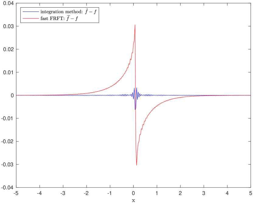
(a) Q=2

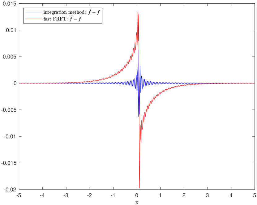
(b) Q=5

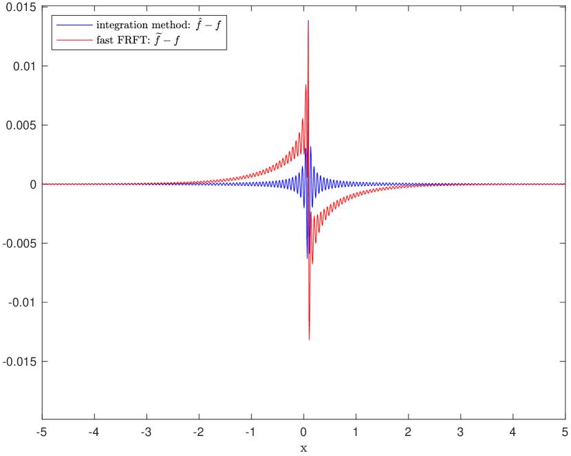
(c) Q=10

Figure 1. Variance-Gamma $(\mu,\delta,\alpha,\theta,\sigma)$ PDF: N=3000 a=100

3. Fast Fractional Fourier Transform (FRFT) and Composite Newton-Cotes Quadrature rules

3.1. Fast Fourier Transform and Fractional Fourier Transform

The Conventional fast Fourier transform (FFT) algorithm is widely used to compute discrete convolutions, discrete Fourier transforms (DFT) of sparse sequence, and to perform high-resolution trigonometric interpolation [5, 1]. The discrete Fourier transforms (DFT) are based on $N^{th}$ roots of unity $e^{-\frac{2\pi i}{N}}$. The generalization of DFT is the fractional Fourier transform, which is based on fractional roots of unity $e^{-2\pi i\alpha}$, where $\alpha$ is an arbitrary complex number.
The fractional Fourier transform is defined on $M$-long sequence ($x_{1}$, $x_{2}$, …, $x_{M}$) as follows

$$G_{k+s}(x,\delta)=\sum_{j=0}^{M-1}\!x_{j}e^{-2\pi ij(k+s)\delta}\hskip 14.22636pt  \hbox{$0\leq k<M$ \quad$0\leq s\leq 1$}$$ (3.1)

Let us have $2j(k+s)=j^{2}+(k+s)^{2}-(k-j+s)^{2}$ , equation (3.1) becomes

$$G_{k+s}(x,\delta) =\sum_{j=0}^{M-1}\!x_{j}e^{-\pi i(j^{2}+(k+s)^{2}-(k-j+s)^{2})\delta}=e^{-\pi i(k+s)^{2}\delta}\sum_{j=0}^{M-1}\!x_{j}e^{-\pi ij^{2}\delta}e^{\pi i(k-j+s)^{2}\delta}$$ (3.2)

$$=e^{-\pi i(k+s)^{2}}\sum_{j=0}^{M-1}\!y_{j}z_{k-j}\hskip 28.45274pt  \hbox{$y_{j}=x_{j}e^{-\pi ij^{2}\delta}$ \quad\quad$z_{j}=e^{\pi i(j+s)^{2}\delta}$}$$

The expression $\sum_{j=0}^{M-1}\!y_{j}z_{k-j}$ is a discrete convolution. Still, we need a circular convolution (i.e., $z_{k-j}=z_{k-j+M}$) to evaluate $G_{k+s}(x,\delta)$. The conversion from discrete convolution to discrete circular convolution is possible by extending the sequence $y$ and $z$ to length $2M$ defined as follows.

$$y_{j} =x_{j}e^{-\pi ij^{2}\delta} \quad z_{j} =e^{\pi i(j+s)^{2}\delta} \quad \hskip 14.22636pt \hbox{$0\leq j<M$}$$ (3.3)

$$y_{j} =0 \quad z_{j} =e^{\pi i(j+s-2M)^{2}\delta} \quad \hskip 14.22636pt  \hbox{$M\leq j<2M$}$$

Taking into account the 2M-long sequence, the previous fractional Fourier transform becomes

$$G_{k+s}(x,\delta)=e^{-\pi i(k+s)^{2}\delta}\sum_{j=0}^{2M-1}\!y_{j}z_{k-j}=e^{-\pi i(k+s)^{2}\delta}{DFT}_{k}^{-1}[{{DFT}_{j}(y){DFT}_{j}(z)}]$$ (3.4)

Where $DFT$ is the Discrete Fourier Transform, and $DFT^{-1}$ is the inverse of $DFT$. For an n-long sequence $z$, we have

$$DFT_{k}(z)=\sum_{j=0}^{N-1}z_{j}e^{-2\pi\frac{jk}{N}}\quad\quad DFT^{-1}_{k}(z)=\frac{1}{N-1}\sum_{j=0}^{N-1}z_{j}e^{2\pi\frac{jk}{N}}$$ (3.5)

This procedure is referred to in the literature as the Fast fractional Fourier Transform Algorithm with a total computational cost of $20Mlog_{2}M+44M$ operations [5].

We assume that $\mathscr{F}[f](y)$ is zero outside the interval $[-\frac{a}{2},\frac{a}{2}]$; $\beta=\frac{a}{M}$ is the step size of the $M$ input values of $\mathscr{F}[f](y)$, defined by $y_{j}=(j-\frac{M}{2})\beta$ for $0\leq j<M$. Similarly, $\gamma$ is the step size of the $M$ output values of $f(t)$, defined by $x_{k}=(k-\frac{M}{2})\gamma$ for $0\leq k<M$. By choosing the step size $\beta$ on the input side and the step size $\gamma$ in the output side, we fix the FRFT parameter $\delta=\frac{\beta\gamma}{2\pi}$ and yield [12] the density function $f$ (4.13) at $x_{k}$.

$$f(x_{k})=\frac{1}{2\pi}\int_{-\infty}^{+\infty}\mathscr{F}[f](y)e^{ix_{k}y}\mathrm{d}y \approx\frac{1}{2\pi}\int_{-a/2}^{a/2}\mathscr{F}[f](y)e^{ix_{k}y}\mathrm{d}y$$

$$=\frac{\gamma}{2\pi}\sum_{j=0}^{N-1}\!\mathscr{F}[f](y_{j})e^{2\pi i(k-\frac{N}{2})(j-\frac{N}{2})\delta}$$

$$=\frac{\gamma}{2\pi}e^{-\pi i(k-\frac{N}{2})N\delta}G_{k}(\mathscr{F}[f](y_{j})e^{-\pi ijN\delta}),-\delta)$$

We have :

$$\hat{f}(x_{k})=\frac{\gamma}{2\pi}e^{-\pi i(k-\frac{N}{2})N\delta}G_{k}(\mathscr{F}[f](y_{j})e^{-\pi ijN\delta},-\delta)\hskip 14.22636pt  \hbox{ $0\leq s<1$}$$ (3.6)

3.2. FRFT of QN-long weighted sequence

The Advanced Fast Fourier Transform (FRFT) algorithm combines the Fast Fractional Fourier (FRFT) algorithm (3.6) and the 12-point rule Composite Newton-Cotes Quadrature (LABEL:eq:l71) to evaluate the inverse Fourier integrals.

We assume that $\mathscr{F}[f](x)$ is zero outside the interval $[-\frac{a}{2},\frac{a}{2}]$, $Q=12$, $m=QN$ and $\beta=\frac{a}{M}$ is the step size of the $M$ input values $\mathscr{F}[f](y)$, defined by $y_{j+Qp}=(Qp+j-\frac{M}{2})\beta$ for $0\leq p<N$ and $0\leq j<Q$. Similarly, the output values of $f(x)$ is defined by $x_{Ql+f+s}=(Ql+f+s-\frac{M}{2})\gamma$ for $0\leq l<N$, $0\leq f<Q$ and $0\leq s\leq 1$.

$$f(x_{Ql+f+s}) =\frac{1}{2\pi}\int_{\infty}^{+\infty}e^{iyx_{Ql+f+s}}F[f](y)dy=\frac{1}{2\pi}\int_{-a/2}^{a/2}e^{iyx_{Ql+f+s}}F[f](y)dy$$ (3.7)

$$=\frac{1}{2\pi}\sum_{p=0}^{N-1}\int_{y_{Qp}}^{y_{Qp+Q}}e^{iyx_{Ql+f+s}}F[f](y)dy\hskip 5.69054pt\hbox{ (composite rule)}$$

Based on the Lagrange interpolating integration over [$x_{Qp}$, $x_{Qp+Q}$][10, 9], we have the following expression.

$$\int_{x_{Qp}}^{x_{Qp+Q}}{e^{iyx_{Ql+f+s}}F[f](x)}dx\approx\beta\sum_{j=0}^{Q}w_{j}{e^{iyx_{Ql+f+s}}F[f](x_{j+Qp})}\\$$ (3.8)

we consider $\widehat{f}(x_{Ql+f+s})$ the approximation of $f(x_{Ql+f+s})$ and the expression (3.7) becomes

$$\widehat{f}(x_{Ql+f+s}) =\frac{\beta}{2\pi}\sum_{p=0}^{N-1}\sum_{j=0}^{Q}w_{j}F[f](y_{j+Qp})e^{ix_{Ql+f+s}y_{j+Qp}}\hskip 14.22636pt  \hbox{ $0\leq s<1$}$$ (3.9)

$$=\frac{\beta}{2\pi}\sum_{j=0}^{Q}\sum_{p=0}^{N-1}{w_{j}F[f](y_{j+Qp})e^{2\pi i\delta(Ql+f+s-\frac{M}{2})(Qp+j-\frac{M}{2})}}\hskip 14.22636pt  \hbox{ $\beta\gamma=2\pi\delta$}$$

$$=\frac{\beta}{2\pi}e^{-\pi i\delta M(Ql+f+s-\frac{M}{2})}G_{Ql+f}(w_{j}\mathscr{F}[f](y_{j+Qp})e^{-\pi i(j+Qp)M\delta}),-\delta)$$

We have a Probability density function as a function of fractional Fourier Transform.

$$\widehat{f}(x_{Ql+f+s})=\frac{\beta}{2\pi}e^{-\pi i\delta M(Ql+f+s-\frac{M}{2})}G_{Ql+f}(w_{j}\mathscr{F}[f](y_{j+Qp})e^{-\pi i(j+Qp)M\delta},-\delta)$$ (3.10)

The Fourier transform function ($\mathscr{F}[f]$) is weighted, and we have a fast Fractional Fourier Transform (FRFT) of a QN-long weighted sequence.

3.3. FRFT of Q-long weighted sequence FRFT of N-long sequence

we consider $\widehat{f}(x_{Ql+f+s})$ the approximation of $f(x_{Ql+f+s})$ and the expression (4.1) becomes

$$\widehat{f}(x_{Ql+f+s}) =\frac{\beta}{2\pi}\sum_{p=0}^{N-1}\sum_{j=0}^{Q}w_{j}F[f](y_{j+Qp})e^{ix_{Ql+f+s}y_{j+Qp}}$$

$$=\frac{\beta}{2\pi}\sum_{j=0}^{Q}w_{j}\sum_{p=0}^{N-1}{F[f](y_{j+Qp})e^{2\pi i\delta(Ql+f+s-\frac{M}{2})(Qp+j-\frac{M}{2})}}\hskip 14.22636pt  \hbox{ $\beta\gamma=2\pi\delta$}$$

$$=\frac{\beta}{2\pi}e^{-\pi i\delta M(Ql+f+s-\frac{M}{2})}\sum_{j=0}^{Q}w_{j}e^{2\pi i\delta(Ql+f+s-\frac{M}{2})j}}\sum_{p=0}^{N-1}{F[f](y_{j+Qp})e^{2\pi i\delta(Ql+f+s-\frac{M}{2})Qp}$$

$$=\frac{\beta}{2\pi}e^{-\pi i\delta M(Ql+f+s-\frac{M}{2})}\sum_{j=0}^{Q}w_{j}G_{l+\frac{f+s}{Q}}(\xi_{p},\delta Q^{2})e^{2\pi i\delta(Ql-\frac{m}{2})j}e^{2\pi i\delta(f+s)j}$$

We have the first fractional Fourier transform (FRFT) on the N-long complex sequence $\{\xi_{p}\}_{0\leq p<N}$

$$G_{l+\frac{f+s}{Q}}(\xi_{p},\alpha_{1}=-\delta Q^{2}) =\sum_{p=0}^{N-1}{\xi_{p}e^{-2\pi i(l+\frac{f+s}{Q})p\alpha_{1}}}\quad\quad\xi_{p}=e^{-\pi iMpQ\delta}F[f](y_{j+Qp})$$ (3.11)

$\widehat{f}(x_{Ql+f+s})$ becomes

$$\widehat{f}(x_{Ql+f+s}) =\frac{\beta}{2\pi}e^{-\pi i\delta M(Ql+f+s-\frac{M}{2})}\sum_{j=0}^{Q}w_{j}G_{l+\frac{f+s}{Q}}(\xi_{p},-\alpha_{1})e^{2\pi i\delta(Ql-\frac{M}{2})j}e^{2\pi i\delta(f+s)j}$$ (3.12)

$$=\frac{\beta}{2\pi}e^{-\pi i\delta M(Ql+f+s-\frac{M}{2})}G_{f+s}(z_{j},\delta)$$

We have the second fractional Fourier transform (FRFT) on the Q-long complex sequence $\{z_{j}\}_{0\leq j\leq Q}$

$$G_{f+s}(z_{j},\alpha_{2}=-\delta) =\sum_{j=0}^{Q}z_{j}e^{-2\pi i(f+s)j\alpha_{2}}\quad\quad z_{j}=w_{j}G_{l+\frac{f+s}{Q}}(\xi_{p},-\alpha_{1})e^{2\pi i\delta(Ql-\frac{M}{2})j}$$ (3.13)

The advanced FRFT - scheme yields the following approximation

$$\widehat{f}(x_{Ql+f+s}) =\frac{\beta}{2\pi}e^{-\pi i\delta M(Ql+f+s-\frac{M}{2})}G_{f+s}(z_{j},-\alpha_{2})$$ (3.14)

$$G_{f+s}(z_{j},\alpha_{2} =-\delta)=\sum_{j=0}^{Q}z_{j}e^{-2\pi i(f+s)j\alpha_{2}}\quad\quad z_{j}=w_{j}G_{l+\frac{f+s}{Q}}(\xi_{p},-\alpha_{1})e^{2\pi i\delta(Ql-\frac{M}{2})j}$$

$$G_{l+\frac{f+s}{Q}}(\xi_{p},\alpha_{1}) =\sum_{p=0}^{N-1}{\xi_{p}e^{-2\pi i(l+\frac{f+s}{Q})p\alpha_{1}}}\quad\quad\xi_{p}=e^{-\pi iMpQ\delta}F[f](y_{j+Qp})$$

(3.15) shows that the fast FRFT of a QN-long weighted sequence is the composite of two fast FRFTs: the fast FRFT of a Q-long weighted sequence and the fast FRFT of an N-long sequence.

$$G_{Ql+f}(w_{j}\mathscr{F}[f](y_{j+Qp})e^{-\pi i(j+Qp)N\delta},-\delta) =G_{f+s}(z_{j},-\alpha_{2})$$ (3.15)

$$z_{j} =w_{j}G_{l+\frac{f+s}{Q}}(\xi_{p},-\alpha_{1})e^{2\pi i\delta(Ql-\frac{M}{2})j}$$

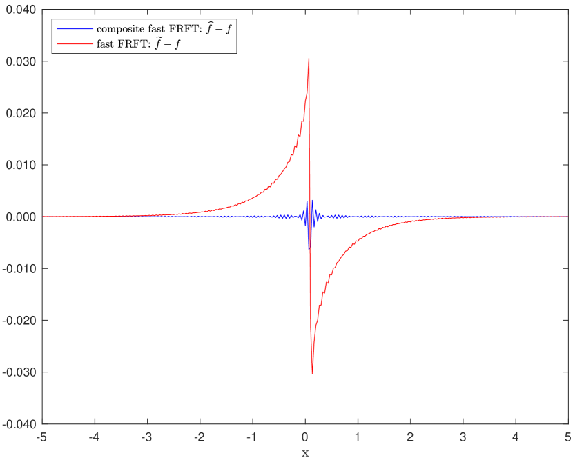
(a) Q=2

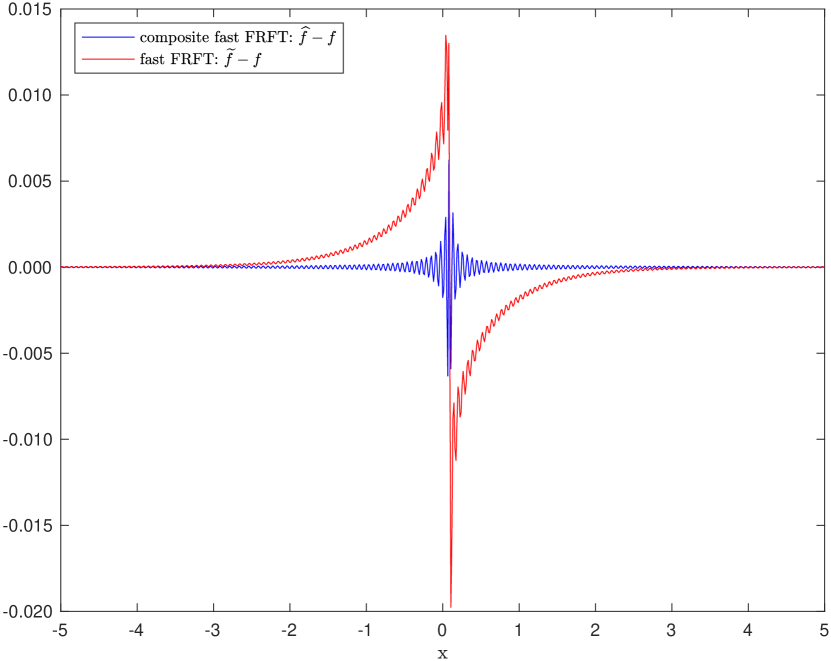
(b) Q=5

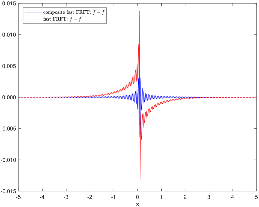
(c) Q=10

Figure 2. Variance-Gamma $(\mu,\delta,\alpha,\theta,\sigma)$ PDF: N=3000 a=100

3.4. FRFT of N-long weighted sequence FRFT of Q-long sequence

we consider $\widehat{f}(x_{Ql+f+s})$ the approximation of $f(x_{Ql+f+s})$ and the expression (4.1) becomes

$$\widehat{f}(x_{Ql+f+s}) =\frac{\beta}{2\pi}\sum_{p=0}^{N-1}\sum_{j=0}^{Q}w_{j}F[f](y_{j+Qp})e^{ix_{Ql+f+s}y_{j+Qp}}$$

$$=\frac{\beta}{2\pi}e^{-\pi i\delta M(Ql+f+s-\frac{M}{2})}\sum_{p=0}^{N-1}e^{2\pi i\delta(Ql+f+s-\frac{M}{2})Qp}\sum_{j=0}^{Q}w_{j}{F[f](y_{j+Qp})e^{2\pi i\delta(Ql-\frac{M}{2})j}}e^{2\pi i\delta(f+s)j}$$

$$=\frac{\beta}{2\pi}e^{-\pi i\delta M(Ql+f+s-\frac{M}{2})}\sum_{p=0}^{N-1}G_{f+s}(z_{j},\delta)e^{-\pi i\delta MQp}e^{2\pi i(l+\frac{f+s}{Q})\delta Q^{2}p}$$

We have the first fractional Fourier transform (FRFT) on the N-long complex sequence $\{z_{j}\}_{0\leq j<Q}$

$$G_{f+s}(z_{j},\alpha_{2}=-\delta)=\sum_{j=0}^{Q}z_{j}e^{-2\pi i(f+s)j\alpha_{2}}\quad\quad z_{j}=w_{j}F[f](y_{j+Qp})e^{2\pi i\delta(Ql-\frac{m}{2})j}$$ (3.16)

$\widehat{f}(x_{Ql+f+s})$ becomes

$$\widehat{f}(x_{Ql+f+s}) =\frac{\beta}{2\pi}e^{-\pi i\delta m(Ql+f+s-\frac{m}{2})}\sum_{p=0}^{N-1}G_{f+s}(z_{j},\delta)e^{-\pi i\delta mQp}e^{2\pi i(l+\frac{f+s}{Q})\delta Q^{2}p}$$ (3.17)

$$=\frac{\beta}{2\pi}e^{-\pi i\delta m(Ql+f+s-\frac{m}{2})}G_{l+\frac{f+s}{Q}}(\xi_{p},\delta Q^{2})$$

We have the second fractional Fourier transform (FRFT) on the Q-long complex sequence $\{\xi_{p}\}_{0\leq p\leq Q}$

$$G_{l+\frac{f+s}{Q}}(\xi_{p},\alpha_{1}=-\delta Q^{2})=\sum_{p=0}^{N-1}{\xi_{p}e^{-2\pi i(l+\frac{f+s}{Q})p\alpha_{1}}}\quad\quad\xi_{p}=G_{f+s}(z_{j},\delta)e^{-\pi i\delta mQp}$$ (3.18)

The advanced FRFT - scheme yields the following approximation

$$\widehat{f}(x_{Ql+f+s}) =\frac{\beta}{2\pi}e^{-\pi i\delta m(Ql+f+s-\frac{m}{2})}G_{f+s}(z_{j},-\alpha_{2})$$ (3.19)

$$G_{f+s}(z_{j},\alpha_{2} =-\delta)=\sum_{j=0}^{Q}z_{j}e^{-2\pi i(f+s)j\alpha_{2}}\quad\quad z_{j}=w_{j}G_{l+\frac{f+s}{Q}}(\xi_{p},-\alpha_{1})e^{2\pi i\delta(Ql-\frac{m}{2})j}$$

$$G_{l+\frac{f+s}{Q}}(\xi_{p},\alpha_{1}) =\sum_{p=0}^{N-1}{\xi_{p}e^{-2\pi i(l+\frac{f+s}{Q})p\alpha_{1}}}\quad\quad\xi_{p}=e^{-\pi impQ\delta}F[f](y_{j+Qp})$$

The results (3.19) are similar to the results (3.14). However, the numerical computation shows that the results (3.19) do not provide the numerical inversion of the Laplace transforms. As shown in Fig 3(a), Fig 3(b), and Fig 3(c), the results (3.19) do not yield a function in the sense each input is not related to exactly one output.

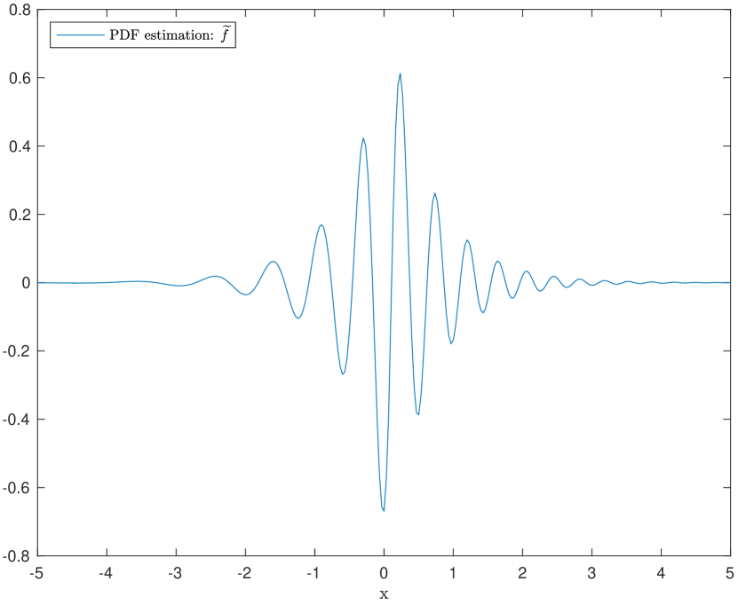
(a) Q=2

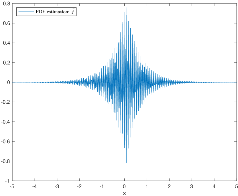
(b) Q=5

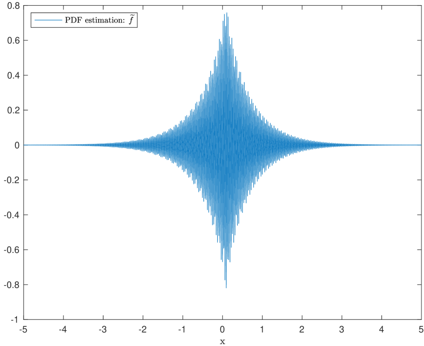
(c) Q=10

Figure 3. Variance-Gamma $(\mu,\delta,\alpha,\theta,\sigma)$ PDF: N=3000 a=100

4. ILLUSTRATION EXAMPLES

4.1. Variance-Gamma VG $(\mu,\delta,\alpha,\theta,\sigma)$ Distribution

In the study, the VG model has five parameters: parameters of location ($\mu$), symmetric ($\delta$), volatility ($\sigma$), and the Gamma parameters of shape ($\alpha$) and scale ($\theta$). The VG model density function is proven to be (4.1).

$$f(y)=\frac{1}{\sigma\Gamma(\alpha)\theta^{\alpha}}\int_{0}^{+\infty}\frac{1}{\sqrt{2\pi\nu}}e^{-\frac{(y-\mu-\delta\nu)^{2}}{2\nu\sigma^{2}}}\nu^{\alpha-1}e^{-\frac{\nu}{\theta}}\,d\nu$$ (4.1)

The VG model density function (4.1) has an analytical expression with a modified Bessel function of the second kind. the expression can be obtained by making some transformations and changing the variable in (4.1).

$$-\frac{(y-\mu-\delta\nu)^{2}}{2\nu\sigma^{2}}-\frac{\nu}{\theta}=\delta(\frac{y-\mu}{\sigma^{2}})-\frac{1}{2\sigma^{2}}(\delta^{2}+\frac{2\sigma^{2}}{\theta})\nu-(\frac{y-\mu}{\sigma^{2}})^{2}\frac{1}{2\nu}$$ (4.2)

(4.1) becomes

$$f(y)=\frac{e^{\delta(\frac{y-\mu}{\sigma^{2}})}}{\sqrt{2\pi}\sigma\Gamma(\alpha)\theta^{\alpha}}\int_{0}^{+\infty}e^{-\frac{1}{2\sigma^{2}}(\delta^{2}+\frac{2\sigma^{2}}{\theta})\nu-(\frac{y-\mu}{\sigma^{2}})^{2}\frac{1}{2\nu}}\nu^{\alpha-\frac{3}{2}}\,d\nu$$ (4.3)

We consider the modified Bessel function of the second kind ($k_{\alpha}(z)$)[13].

$$k_{\alpha}(z)=\frac{1}{2}(\frac{1}{2}z)^{\alpha}\int_{0}^{+\infty}e^{(-t-\frac{z^{2}}{4t})}\frac{1}{t^{\alpha+1}}\,dt\quad\quad|arg(z)|\leq\frac{\pi}{4}$$ (4.4)

$k_{\alpha}(z)$ is the second kind of solution for the modified Bessel’s equation.

$$z^{2}\frac{d^{2}w}{dz^{2}}+z\frac{dw}{dz}-(z^{2}+\alpha^{2})w=0$$ (4.5)

By changing variable, $u=\frac{1}{2\sigma^{2}}(\delta^{2}+\frac{2\sigma^{2}}{\theta})\nu$, and (4.7) becomes

$$f(y)=\frac{2e^{\delta(\frac{y-\mu}{\sigma^{2}})}}{\sqrt{2\pi}\sigma\Gamma(\alpha)\theta^{\alpha}}\left(\frac{|y-\mu|}{\sqrt{\delta^{2}+\frac{2\sigma^{2}}{\theta}}}\right)^{\alpha-\frac{1}{2}}k_{-\alpha+\frac{1}{2}}\left(\frac{\sqrt{\delta^{2}+\frac{2\sigma^{2}}{\theta}}|y-\mu|}{\sigma^{2}}\right)$$ (4.6)

Table 2. FRFT Maximum Likelihood VG Parameter Estimation

Model	$\mu$	$\delta$	$\sigma$	$\alpha$	$\theta$
VG	$0.08476896$	$-0.0577418$	$1.02948292$	$0.88450029$	$0.93779517$

Table 3 presents the estimation results of the five parameters $(\mu,\delta,\alpha,\theta,\sigma)$ of the Variance-Gamma variable. The data comes from the daily S$\&$P 500 historical data (adjustment for splits and dividends) and spans from January 4, 2010, to December 30, 2020. See [12, 14, 15, 16, 17] for more details.

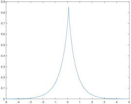
Figure 4. VG Model ($f(y)$): $\hat{\mu}=0.0848$, $\hat{\delta}=-0.0577$, $\hat{\sigma}=1.0295$, $\hat{\alpha}=0.8845$, $\hat{\theta}=0.9378$

The VG density function in (4.6) shows continuity at $\mu$ but not derivative at the same value. Fig 4.6 illustrates the continuity end non-derivative at $\mu$ by the pick at $\mu$. The expression of $f(\mu)$ can be determined analytically.

$$f(\mu) =\frac{1}{\sqrt{2\pi}\sigma\Gamma(\alpha)\theta^{\alpha}}\int_{0}^{+\infty}e^{-\frac{1}{2\sigma^{2}}(\delta^{2}+\frac{2\sigma^{2}}{\theta})\nu}\nu^{\alpha-\frac{3}{2}}d\nu$$ (4.7)

$$=\frac{1}{\sqrt{2\pi}\sigma\Gamma(\alpha)\theta^{\alpha}}\frac{\Gamma(\alpha-\frac{1}{2})}{(\frac{1}{2\sigma^{2}}(\delta^{2}+\frac{2\sigma^{2}}{\theta}))^{\alpha-\frac{1}{2}}}=\frac{1}{\sqrt{2\pi\theta}\sigma}\frac{1}{(1+\frac{\theta}{2}\frac{\delta^{2}}{\sigma^{2}})^{\alpha-\frac{1}{2}}}\frac{\Gamma(\alpha-\frac{1}{2})}{\Gamma(\alpha)}$$

We have the following expression

$$f(\mu)=\frac{1}{\sqrt{2\pi\theta}\sigma}\frac{1}{(1+\frac{\theta}{2}\frac{\delta^{2}}{\sigma^{2}})^{\alpha-\frac{1}{2}}}\frac{\Gamma(\alpha-\frac{1}{2})}{\Gamma(\alpha)}$$ (4.8)

For the VG parameter data: $\hat{\mu}=0.0848$, $\hat{\delta}=-0.0577$, $\hat{\sigma}=1.0295$, $\hat{\alpha}=0.8845$, $\hat{\theta}=0.9378$, we have

$$\hat{f}(\hat{\mu})\approx 0.8552$$ (4.9)

The Variance Gamma distribution is infinitely divisible, and the Fourier transform function has explicit closed form (4.10).

$$\mathscr{F}[f](x) =\frac{e^{-i\mu x}}{\left(1+\frac{1}{2}\theta\sigma^{2}x^{2}+i\delta\theta x\right)^{\alpha}}\quad\quad \widehat{f}(y)=\frac{1}{2\pi}\int_{-\infty}^{+\infty}e^{iyx+\Psi(-x)}dx$$ (4.10)

Based on the integral approximation proposition 1.1 in (2.6), the numerical estimation of density function (4.10) becomes

$$\hat{f}(x) =\beta\sum_{p=0}^{N-1}\sum_{j=0}^{Q}W_{j}e^{(iy_{j+Qp}x)}F[f](y_{j+Qp})\hskip 14.22636pt\hbox{Integral approximation}$$ (4.11)

$$\widetilde{f}(x_{k}) =\frac{\gamma}{2\pi}e^{-\pi i(k-\frac{N}{2})N\delta}G_{k}(\mathscr{F}[f](y_{j})e^{-\pi ijN\delta},-\delta)\hskip 14.22636pt\hbox{fast FRFT}$$

$$\widehat{f}(x_{Ql+f}) =\frac{\beta}{2\pi}e^{-\pi i\delta M(Ql+f-\frac{M}{2})}G_{f+s}(z_{j},-\alpha_{2})\hskip 14.22636pt\hbox{composite fast FRFT}$$

Taking into account the numerical density function in (4.11); we can numerically compute the absolute error ($f-\widehat{f}$).

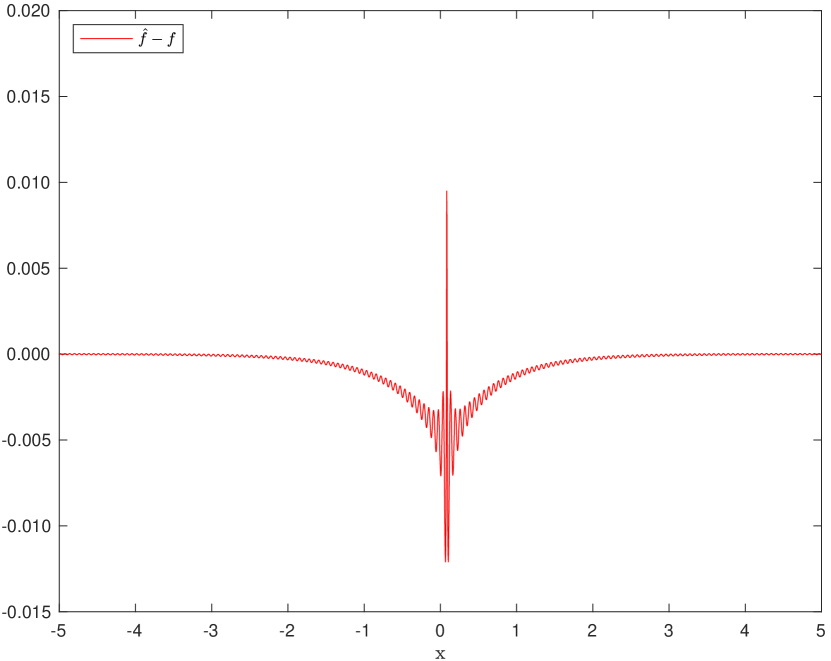
(a) Integration method

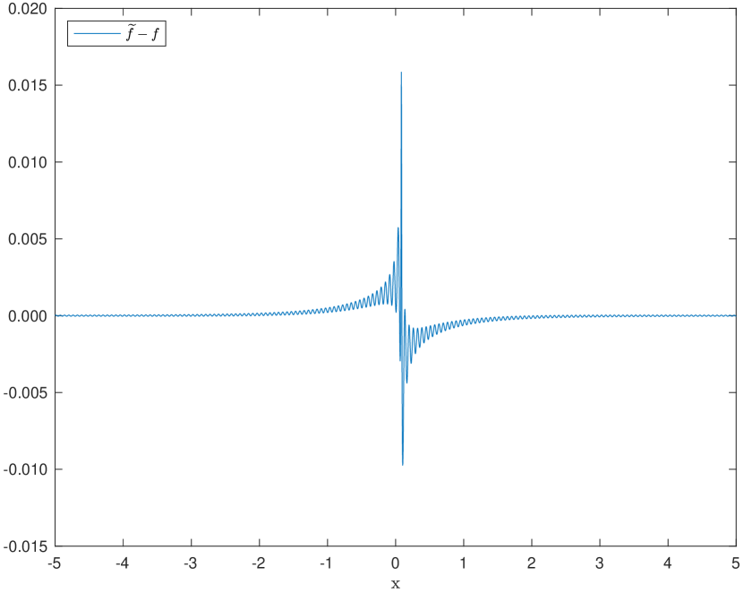
(b) fast FRFT

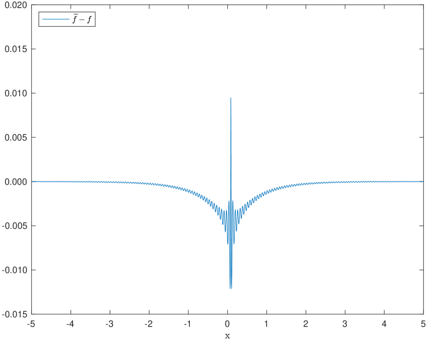
(c) composite fast FRFT

Figure 5. Variance-Gamma(VG) PDF: Q=5 N=3000 a=200

4.2. Generalized Tempered Stable (GTS)($\beta_{+}$, $\beta_{-}$, $\alpha_{+}$,$\alpha_{-}$, $\lambda_{+}$, $\lambda_{-}$) Distribution

We consider a GTS variable $Y=\mu+X=\mu+X_{+}-X_{-}\sim GTS(\textbf{$\mu$},\textbf{$\beta_{+}$},\textbf{$\beta_{-}$},\textbf{$\alpha_{+}$},\textbf{$\alpha_{-}$},\textbf{$\lambda_{+}$},\textbf{$\lambda_{-}$})$ with $X_{+}\sim TS(\textbf{$\beta_{+}$},\textbf{$\alpha_{+}$},\textbf{$\lambda_{+}$},\textbf{$\lambda_{-}$})$ and $X_{-}\sim TS(\textbf{$\beta_{-}$},\textbf{$\alpha_{-}$},\textbf{$\lambda_{-}$},\textbf{$\lambda_{-}$})$. The characteristic exponent can be written [18, 14, 19]

$$\Psi(\xi)=\mu\xi i+\alpha_{+}\Gamma(-\beta_{+})\left((\lambda_{+}-i\xi)^{\beta_{+}}-{\lambda_{+}}^{\beta_{+}}\right)+\alpha_{-}\Gamma(-\beta_{-})\left((\lambda_{-}+i\xi)^{\beta_{-}}-{\lambda_{-}}^{\beta_{-}}\right)$$ (4.12)

Table 3 presents the estimation results of the seven parameters $(\textbf{$\beta_{+}$},\textbf{$\beta_{-}$},\textbf{$\alpha_{+}$},\textbf{$\alpha_{-}$},\textbf{$\lambda_{+}$},\textbf{$\lambda_{-}$})$ Generalized Tempered Stable (GTS) Distribution. The data comes from the daily GTS historical data (adjustment for splits and dividends) and spans from April 28, 2013, to June 22, 2023. See [18, 14, 19] for more details.

Table 3. FRFT Maximum Likelihood GTS Parameter Estimation

Model	$\mu$	$\beta_{+}$	$\beta_{-}$	$\alpha_{+}$	$\alpha_{-}$	$\lambda_{+}$	$\lambda_{-}$
GTS	-0.693477	0.682290	0.242579	0.458582	0.414443	0.822222	0.727607

The characteristic function of the GTS variable has the following expression

$$\vartheta(\xi)=E\left[e^{iY\xi}\right]=e^{\Psi(\xi)}$$ (4.13)

And the GTS density function ($f$) generated by the characteristic function (4.13) and Fourier Transform ($F(f)$) can be written [14] as follows:

$$F[f](\xi)=\vartheta(-\xi)\quad\quad f(y)=\frac{1}{2\pi}\int_{-\infty}^{+\infty}e^{iyx+\Psi(-x)}dx$$ (4.14)

Based on the Conventional FRFT and the FRFT of Q-long weighted sequence FRFT of N-long sequence, (4.10) becomes

$$\widetilde{f}(x_{k}) =\frac{\gamma}{2\pi}e^{-\pi i(k-\frac{N}{2})N\delta}G_{k}(\mathscr{F}[f](y_{j})e^{-\pi ijN\delta},-\delta)\hskip 28.45274pt\hbox{FRFT without weight}$$

$$\widehat{f}(x_{Ql+f}) =\frac{\beta}{2\pi}e^{-\pi i\delta M(Ql+f-\frac{M}{2})}G_{f+s}(z_{j},-\alpha_{2})\hskip 14.22636pt\hbox{Composite fast FRFT}$$

The GTS probability density function has neither a closed form nor an analytic expression. We have the absolute error ($\widehat{f}-\widetilde{f}$), which is the difference between the estimations composite fast FRFT ($\widehat{f}$) and fast FRFT without weight($\widetilde{f}$). As shown in Fig 6, the absolute error ($\widehat{f}-\widetilde{f}$) is almost zero.

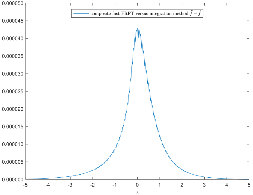
(a) Integration method (Q=5)

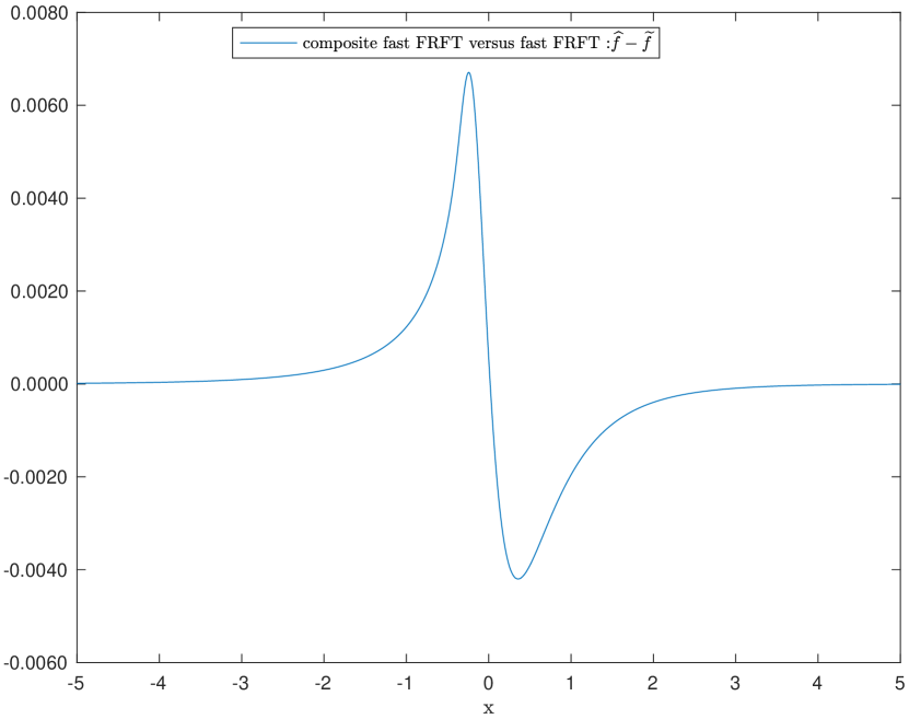
(b) fast FRFT(Q=5)

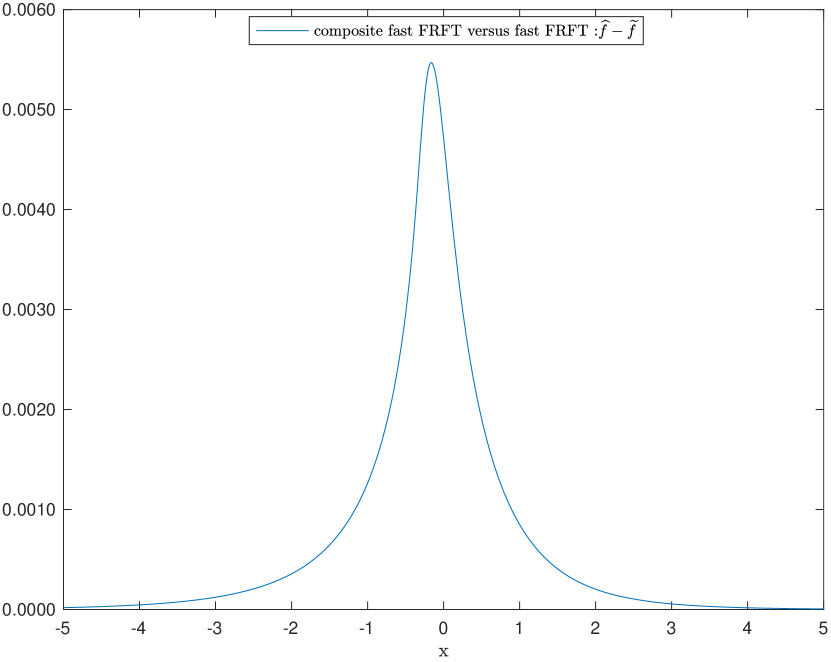
(c) fast FRFT(Q=20)

Figure 6. Generalized Tempered Stable (GTS) PDF: N=3000 a=100

Analytically, the GTS probability density function does not have a closed form, but Fig 6 shows that the GTS probability density function is smooth, which is differentiable at least one time.

5. Conclusion

The closed composite Newton-Cotes quadrature rule and the Fast Fractional Fourier Transform (FRFT) algorithm are reviewed in the paper. Both schemes are combined to yield the fast Fractional Fourier Transform (FRFT) of a QN-long weighted sequence. It is shown that the fast Fractional Fourier transform (FRFT) of a QN-long weighted sequence is the composite of two fast FRFTs: the fast FRFT of a Q-long weighted sequence and the fast FRFT of an N-long sequence. By changing the order of composition, we have another theoretical alternative, the composite of the fast FRFT of an N-long weighted sequence and the fast FRFT of a Q-long sequence. However, the numerical computation shows that the composition does not provide the numerical inversion of the Fourier and Laplace transforms. The composite of the two fast FRFTs (the fast FRFT of a Q-long weighted sequence and the fast FRFT of an N-long sequence) scheme was applied to estimate the probability density function of the Variance-Gamma VG $(\mu,\delta,\alpha,\theta,\sigma)$ distribution and the Generalized Tempered Stable (GTS)($\beta_{+}$, $\beta_{-}$, $\alpha_{+}$,$\alpha_{-}$, $\lambda_{+}$, $\lambda_{-}$) Distribution. Compared to the non-weighted fast FRFT, the composite fast FRFT provides more accurate results with a small sample size, and the accuracy increases with the number of weights (Q). The composite fast FRFT performs relatively well when the inversion of Fourier and Laplace transforms has singularities. This was the case for the VG probability density function, which is continuous but non-derivative at $x=\mu$. Analytically, the GTS probability density function does not have a closed form, but the numerical results show that the GTS probability density function is smooth, which is differentiable at least one time.

References

• [1] David H Bailey and Paul N Swarztrauber. A fast method for the numerical evaluation of continuous fourier and laplace transforms. SIAM Journal on Scientific Computing, 15(5):1105–1110, 1994.
• [2] Lin Mei, XueJun Sha, QinWen Ran, and NaiTong Zhang. Research on the application of 4-weighted fractional fourier transform in communication system. Science China Information Sciences, 53:1251–1260, 2010.
• [3] Xingpeng Yang, Qiaofeng Tan, Xiaofeng Wei, Yong Xiang, Yingbai Yan, and Guofan Jin. Improved fast fractional-fourier-transform algorithm. J. Opt. Soc. Am. A, 21(9):1677–1681, Sep 2004.
• [4] Lin Mei, XueJun Sha, QinWen Ran, and NaiTong Zhang. Research on the application of 4-weighted fractional fourier transform in communication system. Science China Information Sciences, 53(6):1251–1260, 2010.
• [5] David H Bailey and Paul N Swarztrauber. The fractional fourier transform and applications. SIAM review, 33(3):389–404, 1991.
• [6] Javier Garcia, David Mas, and Rainer G Dorsch. Fractional-fourier-transform calculation through the fast-fourier-transform algorithm. Applied optics, 35(35):7013–7018, 1996.
• [7] Steven C Chapra. Numerical methods for engineers. Mcgraw-hill, 2010.
• [8] EO Tuck. A simple ”filon-trapezoidal” rule. Mathematics of Computation, 21(98):239–241, 1967.
• [9] A. H. Nzokem. Numerical solution of a gamma - integral equation using a higher order composite newton-cotes formulas. Journal of Physics: Conference Series, 2084(1):012019, nov 2021.
• [10] A. H. Nzokem. Stochastic and Renewal Methods Applied to Epidemic Models. PhD thesis, York University , YorkSpace institutional repository, 2020.
• [11] Dan Kalman. The generalized vandermonde matrix. Mathematics Magazine, 57(1):15–21, 1984.
• [12] A. H. Nzokem. Fitting infinitely divisible distribution: Case of gamma-variance model. arXiv.2104.07580[stat.ME], 2021.
• [13] Nist digital library of mathematical functions. https://dlmf.nist.gov, Release 1.1.11 of 2023-09-15. F. W. J. Olver, A. B. Olde Daalhuis, D. W. Lozier, B. I. Schneider, R. F. Boisvert, C. W. Clark, B. R. Miller, B. V. Saunders, H. S. Cohl, and M. A. McClain, eds.
• [14] A. H. Nzokem. European option pricing under generalized tempered stable process: Empirical analysis. arXiv.2304.06060[q-fin.PR], 2023.
• [15] A. H. Nzokem. Gamma variance model: Fractional fourier transform (FRFT). Journal of Physics: Conference Series, 2090(1):012094, nov 2021.
• [16] A.H. Nzokem and V.T. Montshiwa. The ornstein–uhlenbeck process and variance gamma process: Parameter estimation and simulations. Thai Journal of Mathematics, 21(3):160–168, Sep. 2023.
• [17] A. H. Nzokem. Pricing european options under stochastic volatility models: Case of five-parameter variance-gamma process. Journal of Risk and Financial Management, 16(1), 2023.
• [18] A. H. Nzokem and V. T. Montshiwa. Fitting generalized tempered stable distribution: Fractional fourier transform (frft) approach. ARXIV.2205.00586[q-fin.ST], 2022.
• [19] A. H. Nzokem. Bitcoin versus s&p 500 index: Return and risk analysis. arXiv.2310.02436 [q-fin.ST], 2023.