Black Holes, Cavities and Blinking Islands

Abstract

Placing a black hole in a cavity is known to be a natural way to study different scales in gravity, issues related to the thermodynamic instability and gravity effective theories. In this paper, we consider the evolution of the entanglement entropy and entanglement islands in the two-sided generalization of the Schwarzschild black hole in a cavity. Introducing a reflecting boundary in the eternal black exteriors we regulate infrared modes of Hawking radiation and find that entanglement entropy saturates at some constant value. This value could be lower than black hole thermodynamic entropy, thus not leading to Page formulation of information paradox. Concerning the entanglement islands, we find a universal effect induced by the boundary presence, which we call “blinking island” – for some time the entanglement island inevitably disappears, thus leading to a short-time information paradox.

1 Introduction

Black holes and their radiation are mysterious objects that still enigma us, and Hawking radiation is surely one of them Hawking:1975vcx ; Hawking:1976ra . Recently, much attention has been drawn to the reformulation of the information paradox, or rather its replacement with the question of entanglement evolution in the form of the Page curve Page:1993wv ; Page:2013dx . This means, that after the characteristic time called Page time entanglement entropy of radiation exceeds thermodynamic entropy Page:1993wv ; Page:2013dx indicating non-unitary evolution.

It has been shown how the entanglement island mechanism Penington:2019npb ; Almheiri:2019psf ; Almheiri:2019hni and the replica wormhole Penington:2019kki ; Almheiri:2019qdq stop the growth of entanglement after Page time. The entanglement island has been studied in the setups of two-dimensional gravity Penington:2019npb ; Almheiri:2019psf ; Almheiri:2019hni ; Almheiri:2019yqk ; Penington:2019kki ; Almheiri:2019qdq ; Chen:2020uac ; Almheiri:2020cfm ; Chen:2020hmv , boundary CFT Rozali:2019day ; Sully:2020pza ; Geng:2021iyq ; Ageev:2021ipd ; Geng:2021mic ; Suzuki:2022xwv ; Hu:2022ymx ; Hu:2022zgy ; BasakKumar:2022stg ; Afrasiar:2022ebi ; Geng:2022dua and moving mirror models Davies:1976hi ; Good:2016atu ; Chen:2017lum ; Good:2019tnf ; Akal:2020twv ; Kawabata:2021hac ; Reyes:2021npy ; Akal:2021foz ; Fernandez-Silvestre:2021ghq ; Akal:2022qei .

Although the rigorous argument for the existence of entanglement islands is made in lower-dimensional models, in higher-dimensional backgrounds it is possible to use the s-wave approximation and study them as well under reasonable assumptions. For the case of Schwarzschild black hole solution this has been done in the paper by Hashimoto, Iizuka and Matsuo Hashimoto:2020cas generalized in different contexts recently Ageev:2022qxv ; Alishahiha:2020qza ; Ling:2020laa ; Matsuo:2020ypv ; Karananas:2020fwx ; Wang:2021woy ; Kim:2021gzd ; Lu:2021gmv ; Yu:2021cgi ; Ahn:2021chg ; Cao:2021ujs ; Azarnia:2021uch ; Arefeva:2021kfx ; He:2021mst ; Yu:2021rfg ; Arefeva:2022cam ; Gan:2022jay ; Azarnia:2022kmp ; Anand:2022mla ; Ageev:2022hqc .

One of the canonical setups to test entanglement dynamics of Hawking radiation and island mechanism is the one involving the eternal black hole – namely the entanglement entropy of infinite regions “collecting” Hawking radiation located in different exteriors. In this paper, we consider the question of what happens if we confine Hawking radiation in each (left and right) exterior with the perfectly reflecting boundary.

Our motivation for such a study is two-fold. The study of the black hole in a cavity introduces a new scale “regulating” spatial infinity and clarifies issues concerning the black hole stability, nucleation, etc York:1986it ; Gross:1982cv . The regulation of the infrared mode in entanglement entropy in the context of entanglement islands has been considered in our recent paper Ageev:2022qxv . Introduction of the boundaries is a reasonable and simple way to regulate infrared issues which can be met in the entanglement entropy of massless fields Yazdi:2016cxn . Also, such a setup may be helpful when considering multi-horizon spacetime like Schwarzschild-de Sitter black hole, where the introduction of boundaries makes it possible to separate thermal radiation from the black hole and cosmological horizons, which have different temperatures Gibbons:1977mu ; Saida:2009ss ; Ma:2016arz . This is our first motivation. The second motivation is to find the simple and convenient model where the island mechanism does not help us to solve the Page formulation of the information paradox. We find that the black hole in the cavity is definitely such a case. The introduction of cavity leads to the disappearance of the island solution for a some time – we call this effect “blinking island”. For a reflecting boundary placed close enough to the horizon, the entanglement entropy does not exceed thermodynamic entropy, thus being healthy from the information paradox viewpoint.

After considering the eternal black hole where each of the exteriors contain the boundary, we modify this setup such that only one exterior region now is equipped with it. This enhances the entanglement dynamics for regions contained only in a single (left or right) wedge. Up to our knowledge such a geometry has not been considered yet. In the case of double-boundary geometry the interpretation in terms of thermofield double state is straightforward. In the case of single boundary the exact description of such a geometry seems to be unclear is full generality. We interpret it as two pairs of distant black holes (one of which confined by the reflecting boundary) connected by some sort of Einstein–Rosen bridge Maldacena:2013xja . If we locate the entangling region (without taking into account island mechanism) only in a single wedge in double-boundary geometry we obtain no time dependence for entanglement entropy. In contrast to this we find that boundary being situated only in a single exterior lead to non-trivial dynamical pattern for entanglement. Also by analogy we find numerically asymmetric blinking island solutions in single-boundary geometry in cases when the time dependence of entanglement entropy corresponds to non-unitary evolution.

The paper is organized as follows. In section 2, we setup the notation, present out path-integral geometries and remind basic formulae from BCFT. Section 3 is devoted to the entanglement entropy dynamics in double-boundary geometry and study of blinking island solution corresponding to it. Then in section 4 similarly we study entanglement and islands in single-boundary geometry. Final section is devoted to conclusions.

2 Setup

In this section we remind basics of entanglement entropy calculation in two-dimensional BCFT, then describe and generalize Hashimoto-Iizuka-Matsuo Hashimoto:2020cas setup concerning entanglement island study in s-wave approximation. We describe two-dimensional geometry corresponding to eternal black hole containing the reflecting boundaries and conformal mappings neccesary to calculate the entanglement entropy.

2.1 Entanglement entropy of matter in BCFT₂

Let us start with a brief reminder of the two-dimensional Euclidean boundary conformal field theory and calculation of the entanglement entropy in such a theory. We consider the theory defined on upper half-plane (UHP), i.e. evolving on the line. The coordinate $x_{1}$ corresponds to the Euclidean time, while $x_{2}$ is the spatial coordinate

$$ds^{2}=dx^{2}_{1}+dx^{2}_{2}=dzd\bar{z},\quad z=x_{1}+ix_{2},\quad x_{1}\in(-\infty,\infty),\quad x_{2}\geq 0,$$ (1)

We are interested in the region $R$ consisting of union of single intervals

$$R=[z_{a_{1}},z_{b_{1}}]\cup\ldots\cup[z_{a_{n}},z_{b_{n}}]$$ (2)

and its entanglement entropy

$$S_{\text{m}}(R)=-\mathop{\mathrm{Tr}}(\rho_{R}\log\rho_{R}),$$ (3)

where $\rho_{R}$ is reduced density matrix for region $R$. Entanglement entropy could be obtained by the replica trick Calabrese:2004eu ; Calabrese:2009qy as

$$S_{\text{m}}(R)=-\lim_{n\to 1}\partial_{n}\left(\mathop{\mathrm{Tr}}\rho^{n}_{R}\right).$$ (4)

The trace in (4) is expressed as a correlation function of twist operators inserted at the bulk endpoints of intervals of region $R$ that do not belong to the boundary $x_{2}=0$

$$\mathop{\mathrm{Tr}}\rho^{n}_{R}=\langle\phi(z_{a_{1}},\bar{z}_{a_{1}})\phi(z_{b_{1}},\bar{z}_{b_{1}})\ldots\phi(z_{a_{n}},\bar{z}_{a_{n}})\phi(z_{b_{n}},\bar{z}_{b_{n}})\rangle_{\text{UHP}}.$$ (5)

If the endpoint of the interval is on the boundary, for example $R=[0,z_{1}]$, then the trace is defined as $\mathop{\mathrm{Tr}}\rho^{n}_{R}=\langle\phi(z_{1},\bar{z}_{1})\rangle_{\text{UHP}}$. The twist operators are primary operators with conformal dimensions $h_{n}=\bar{h}_{n}=c/24(n-1/n)$, where $c$ is the central charge Calabrese:2009qy .

We consider the particular BCFT₂ given by $c$ copies of two-dimensional free massless Dirac fermions. The Dirac field is given by the doublet of the left and right moving components

$$\psi(x_{1},x_{2})=\bigg{(}\begin{array}[]{c}\psi_{1}(x_{1},x_{2})\\ \psi_{2}(x_{1},x_{2})\\ \end{array}\bigg{)}=\bigg{(}\begin{array}[]{c}\psi_{1}(z)\\ \psi_{2}(\bar{z})\\ \end{array}\bigg{)}.$$ (6)

We choose the boundary conditions preserving the conformal invariance of the theory and corresponding to the vanishing of the energy and momentum flow through the boundary Cardy:1984bb ; Cardy:1986gw ; Cardy:1989ir . There are two explicit boundary conditions that satisfy this requirement for massless free Dirac fermions on UHP Mintchev:2020uom ; Rottoli:2022plr :

$$\psi_{1}(x_{1},0)=e^{i\alpha_{v}}\psi_{2}(x_{1},0),\qquad\alpha_{v}\in[0,2\pi),\,\,x_{1}\in(-\infty,\infty),$$ (7)

or

$$\psi_{1}(x_{1},0)=e^{-i\alpha_{a}}\psi^{*}_{2}(x_{1},0),\qquad\alpha_{a}\in[0,2\pi),\,\,x_{1}\in(-\infty,\infty).$$ (8)

These boundary conditions correspond to the transition of the left moving component to the right one, which can be interpreted as perfectly reflecting boundary conditions. The entanglement entropy of a region (2) is given by Kruthoff:2021vgv ; Rottoli:2022plr

$$S(R)= \frac{1}{3}\sum^{n}_{i,j=1}\log|z_{a_{i}}-z_{b_{j}}|-\frac{1}{3}\sum^{n}_{i<j}\log|z_{a_{i}}-z_{a_{j}}||z_{b_{i}}-z_{b_{j}}|-n\log\varepsilon$$ (9)

$$+ \frac{1}{6}\sum^{n}_{i,j=1}\log|z_{a_{i}}-\bar{z}_{a_{j}}||z_{b_{i}}-\bar{z}_{b_{j}}|-\frac{1}{6}\sum^{n}_{i,j=1}\log|z_{a_{i}}-\bar{z}_{b_{j}}||z_{b_{i}}-\bar{z}_{a_{j}}|,$$

where $\varepsilon$ is UV cutoff. The entropy (9) does not depend on the choice of the boundary condition (7) or (8) and on the phase $\alpha_{v,a}$ Mintchev:2020uom ; Rottoli:2022plr .

The technique for calculating correlation functions in (B)CFT₂ is mostly applicable within the framework of the Euclidean spacetime, that is why we started with the Euclidean case. But at the end of the calculation we perform analytic continuation to Lorentzian time.

If vacuum state of BCFT₂ is defined on the non-empty simply connected open subset of the complex plane $\Omega$ that does not coincide with UHP, then according to the Riemann mapping theorem there is a conformal transformation

$$z:\Omega\to\text{UHP},\quad z=z(w),\quad\bar{z}=\bar{z}(\bar{w}).$$ (10)

The correlation function of twist operators then transforms as

$$\langle\phi(w_{1},\bar{w}_{1})\ldots\phi(w_{m},\bar{w}_{m})\rangle_{\Omega}=\prod\limits_{j=1}^{m} \left(\frac{dz}{dw}\right)^{h_{n}}\Big{|}_{w=w_{j}}\left(\frac{d\bar{z}}{d\bar{w}}\right)^{\bar{h}_{n}}\Big{|}_{\bar{w}=\bar{w}_{j}}$$ (11)

$$\times \langle\phi(z_{1},\bar{z}_{1})\ldots\phi(z_{m},\bar{z}_{m})\rangle_{\text{UHP}}.$$

Entanglement entropies in flat $ds^{2}=dwd\bar{w}$ and curved $ds^{2}=e^{2\rho(w,\bar{w})}dwd\bar{w}$ two-dimensional spacetimes are related by Weyl transformation $ds^{2}\to e^{2\rho}ds^{2}$

$$S_{\text{m}}\Big{|}_{ds^{2}=e^{2\rho(w,\bar{w})}dwd\bar{w}}=S_{\text{m}}\Big{|}_{ds^{2}=dwd\bar{w}}+\frac{c}{6}\sum_{i=1}^{m}\log e^{\rho(w_{i},\bar{w}_{i})}$$ (12)

The calculation of entanglement entropy $S_{\text{m}}$ of matter theory in a higher-dimensional curved spacetime is an extremely challenging problem. For the study of entanglement islands in Hashimoto:2020cas one proposed to consider the s-wave approximation to overcome difficulties related to higher dimensional geometries (Schwarzschild black hole). So following Hashimoto:2020cas for spherically symmetric geometries of the form

$$ds^{2}=e^{2\rho(w,\bar{w})}dwd\bar{w}+r^{2}d\Omega_{d}^{2}$$ (13)

in what follows we effectively neglect the spherical part of the metric and consider two-dimensional (B)CFT on the rest of the spacetime

$$ds^{2}=e^{2\rho(w,\bar{w})}dwd\bar{w},$$ (14)

assuming that the obtained results captures all main features of dynamics on the higher-dimensional original background.

2.2 Geometry, introduction of the boundaries and path-integral

Our main geometry to study is given by the metric of the four-dimensional Schwarzschild black hole

$$ds^{2}=-f(r)dt^{2}+\frac{dr^{2}}{f(r)}+r^{2}d\Omega_{2}^{2},\qquad f(r)=1-\frac{r_{h}}{r},$$ (15)

at $r>r_{h}$, $-\infty<t<\infty$, where $r_{h}=2GM$ denotes the black hole horizon, $M$ is the mass of the black hole, $G$ is the gravitational constant and $d\Omega_{2}^{2}$ is the angular part of the metric. As we already mentioned in the previous section, in what follows we consider only the two-dimensional part of the metric (15) relying on the s-wave approximation. Within its framework omitting the angular variables, introducing Kruskal coordinates

$$U=-\frac{1}{\kappa_{h}}\,e^{-\kappa_{h}(t-r_{*}(r))},\quad V=\frac{1}{\kappa_{h}}\,e^{\kappa_{h}(t+r_{*}(r))},\,\,\,\,\kappa_{h}=1/2r_{h}$$ (16)

we study two-dimensional metric of the form

$$ds^{2}=-e^{2\rho(r)}dUdV,\quad e^{2\rho(r)}=f(r)e^{-2\kappa_{h}r_{*}(r)}.$$ (17)

where $r_{*}(r)$ is tortoise coordinate given by $r_{*}(r)=r+r_{h}\log|r-r_{h}|/r_{h}$

The transformation between Schwarzschild and Kruskal coordinates (16) can be analytically extended to the region $-\infty<U,V<\infty$ with the constraint $UV<1/\kappa^{2}_{h}$, which is associated with the physical singularities of the past and the future. It is convenient now to relate Kruskal coordinates to timelike $T$ and spacelike $X$ variables

$$U=T-X,\qquad V=T+X.$$ (18)

expressed in terms of Schwarzschild coordinates as

$$T=\pm\frac{e^{\kappa_{h}r_{*}(r)}}{\kappa_{h}}\sinh\kappa_{h}t,\qquad X=\pm\frac{e^{\kappa_{h}r_{*}(r)}}{\kappa_{h}}\cosh\kappa_{h}t,$$ (19)

where the upper (lower) sign corresponds to the right (left) wedge.

As mentioned in the previous section we assume to deal with the calculations of entanglement entropy which is well defined in the Euclidean version of the metric. We Wick rotate Kruskal time $T=-i{\cal T}$ and this also defines the Euclidean Schwarzschild time $\tau=it$ periodic with a period of $2\pi/\kappa_{h}$. The coordinate transformation (19) now takes the form

$${\cal{T}}=\pm\frac{e^{\kappa_{h}r_{*}(r)}}{\kappa_{h}}\sin\kappa_{h}\tau,\qquad X=\pm\frac{e^{\kappa_{h}r_{*}(r)}}{\kappa_{h}}\cos\kappa_{h}\tau.$$ (20)

and left (right) half-plane $X<0$ ($X>0$) corresponds to the left (right) wedge of Lorentzian black hole.

 

From the identity

$$X^{2}+{\cal T}^{2}=\frac{e^{2\kappa_{h}r_{*}(r)}}{\kappa^{2}_{h}},\qquad\tan\kappa_{h}\tau=\frac{{\cal T}}{X},$$ (21)

it is straightforward to see that in the (${\cal T}$, $X$) plane curves $r=\text{const}$ correspond to circles centered at the point ${\cal T}=X=0$ and $\tau=\text{const}$ to the straight lines passing through this point. We consider the exterior of the Euclidean black hole, i.e. $r\geq r_{h}$, and the origin of the (${\cal T}$, $X$) plane corresponds to $r=r_{h}$.

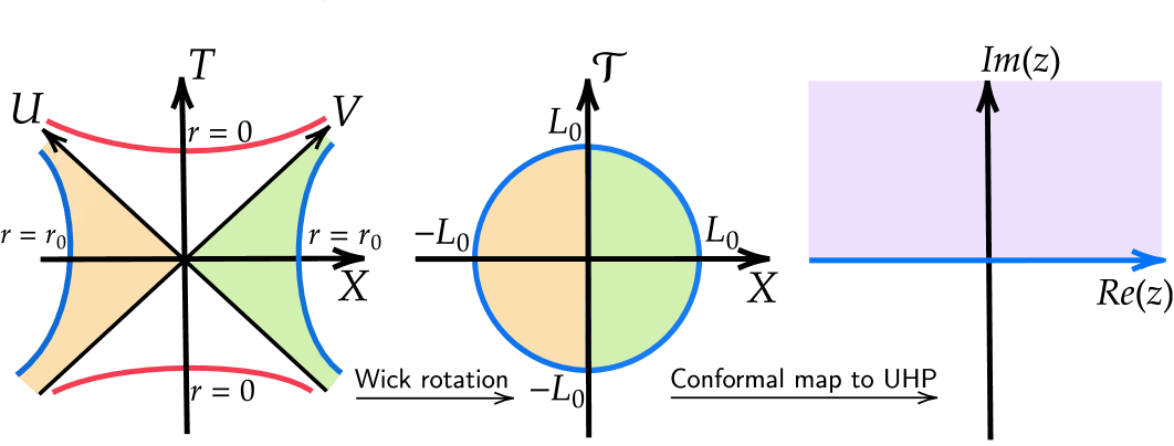
Figure 1: Lorentzian (left) and Euclidean (center) Kruskal diagram of a two-sided Schwarzschild black hole in the presence of two symmetric boundaries at $r=r_{0}$ drawn in blue. The Euclidean Kruskal diagram corresponds to the interior of the disk, that maps conformally to the upper half-plane (right).

We introduce a complex coordinates

$$w=X+i{\cal T},\qquad\bar{w}=X-i{\cal T},$$ (22)

and in this coordinates the Euclidean version of the metric (17) has the form

$$ds^{2}=e^{2\rho(w,\bar{w})}dwd\bar{w},\qquad e^{2\rho(w,\bar{w})}=\frac{W(e^{-1}\kappa^{2}_{h}w\bar{w})}{\kappa^{2}_{h}w\bar{w}\left[1+W(e^{-1}\kappa^{2}_{h}w\bar{w})\right]},$$ (23)

where $W(x)$ is Lambert W function. Total geometry given by (23) (i.e. at $-\infty<{\cal T},X<\infty$) is just the complex plane endowed with the non-trivial metric.

Now we introduce spherically symmetric boundary at the radial coordinate $r\leavevmode\nobreak\ =\leavevmode\nobreak\ r_{0}$, where $r_{0}>r_{h}$, in the analytically extended Schwarzschild geometry. Quantum field (Dirac fermions) now are restricted by the boundary at $r<r_{0}$ via reflecting boundary condition being imposed. We consider two ways to introduce a boundary:

• Two boundaries both in the right and left wedges are located at the same radial coordinate. The Euclidean geometry in the plane $({\cal T},X)$ corresponds to the interior of a disk with the radius $L_{0}=e^{\kappa_{h}r_{*}(r_{0})}/\kappa_{h}$, see Fig.1

• The boundary is located only in the one of the wedges, for examples in the right one for concreteness. The Euclidean geometry in the plane $({\cal T},X)$ corresponds to the union of left half-plane $X<0$ and the interior of a semi-disk in the right half-plane $X>0$ with the radius $L_{0}=e^{\kappa_{h}r_{*}(r_{0})}/\kappa_{h}$, see Fig.2

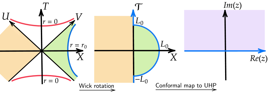
Figure 2: Lorentzian (left) and Euclidean (center) Kruskal diagram of a two-sided Schwarzschild black hole in the presense of boundary, drawn in blue, at radius $r=r_{0}$ only in the right wedge. The Euclidean Kruskal digram corresponds to the union of the interior of the half-disk and the left half-plane, that maps conformally to the upper half-plane (right).

From the path-integral point of view the wavefunctional of our interest is given by the integration over the geometry part with ${\cal T}<0$, i.e. over the lower half of the disk from Fig.1 (for the case of symmetric boundaries). For the single boundary located in the right wedge path integral defining wavefunction is performed over the union of the lower left quadrant and the lower half of the half-disk (${\cal T}<0$ region in Fig.2).

 

As our ultimate goal is to study the entanglement entropy the next step is to perform conformal mapping of the Euclidean geometry given by the central picture in Fig.1 or Fig.2 to the upper half-plane with non-trivial curved metric and then implement Weyl transformation to the flat metric upper half-plane. In this way we obtain explicit form of the entanglement entropy given by the composition of transformation rules for conformal mappings (11) and Weyl transformations (12). The map from the interior of the disk with radius $L_{0}$ to the UHP is defined by

$$z=i\frac{L_{0}+w}{L_{0}-w},\qquad\bar{z}=-i\frac{L_{0}+\bar{w}}{L_{0}-\bar{w}}.$$ (24)

In its turn the map from the union of left half-plane $X<0$ and the interior of a semi-disk in the right half-plane $X>0$ (see Fig.2) with the radius $L_{0}$ to the UHP is given by

$$z=e^{2\pi i/3}\left(\frac{L_{0}+iw}{L_{0}-iw}\right)^{\frac{2}{3}},\qquad\bar{z}=e^{-2\pi i/3}\left(\frac{L_{0}-i\bar{w}}{L_{0}+i\bar{w}}\right)^{\frac{2}{3}}.$$ (25)

Finally let us briefly comment on the possible interpretations of the states under consideration. For the boundaries located symmetrically in the left and right wedges one can refer to the thermofield interpretation of the eternal black hole described by the entangled thermofield double state at $t=0$

$$|\Psi\rangle=\sum_{n}e^{-\beta E_{n}/2}|n\rangle_{L}|n\rangle_{R}$$ (26)

where $|n\rangle_{L,R}$ are the eigenstates with energy $E_{n}$ of the matter theory Hamiltonian in the left and right wedges, $\beta=\kappa_{h}/2\pi$ is the inverse temperature of the black hole.

In this interpretation, the time evolution is upward in both left and right wedges with hamiltonian

$$H_{tot}=H_{L}+H_{R}.$$ (27)

While the state with symmetric boundaries is quite clear from thermofield intepretation point of view, a similar interpretation of the state for single boundary geometry does not seem to be valid due to the lack of symmetry of the right and left wedges.

2.3 Generalized entropy functional

Recently, it was shown that the expected behavior of the Page curve emerges from the island proposal Almheiri:2019hni ; Penington:2019npb ; Almheiri:2019qdq . The reduced density matrix of Hawking radiation collected in $R$ is defined by tracing out the states in the complement region $\overline{R}$, which includes the black hole interior. The island mechanism prescribes that the states in some regions ${I\subset\overline{R}}$, called entanglement islands, are to be excluded from tracing out.

The island contribution can be taken into account via the generalized entropy functional defined as Penington:2019kki ; Almheiri:2019qdq

$$S_{\text{gen}}[I,R]=\frac{\operatorname{Area}(\partial I)}{4G}+S_{\text{m}}(R\cup I).$$ (28)

Here $\partial I$ denotes the boundary of the entanglement island, $G$ is Newton’s constant, and $S_{\text{m}}$ is the entanglement entropy of conformal matter. One should extremize this functional over all possible island configurations

$$S^{\text{ext}}_{\text{gen}}[I,R]=\underset{\partial I}{\operatorname{ext}}\,\Big{\{}S_{\text{gen}}[I,R]\Big{\}},$$ (29)

and then choose the minimal one

$$S(R)=\underset{\partial I}{\text{min}}\,\Big{\{}S^{\text{ext}}_{\text{gen}}[I,R]\Big{\}}.$$ (30)

Note that the entropy of conformal matter $S_{\text{m}}$ is proportional to the number of fields $c$, while it is believed that the area term in the case of a nontrivial island configuration is proportional to $r^{2}_{h}/G$. Since the area term is the leading classical contribution and the entropy of conformal matter is a quantum correction, we impose the constraint $cG/r^{2}_{h}\ll\leavevmode\nobreak\ 1$ (or, equivalently, $cG\kappa^{2}_{h}\ll 1$). Also, this condition allows us to neglect the backreaction effect of matter fields on geometry.

3 Symmetrical boundaries in both exteriors

Now let us study the first proposed in the setup geometries – black hole bounded by two symmetric reflecting boundaries. We calculate the entanglement entropy of the region $R_{2}$, which is the union of two intervals located between bulk points $\mathbf{b}_{\pm}$ and the boundary in the corresponding left/right wedge (magenta curves in Fig.3). In the island phase we assume the inclusion of the island region $I_{2}$ given by the “interval” between two points $\mathbf{a}_{-}$ and $\mathbf{a}_{+}$ in different wedges (green curves in Fig.3)

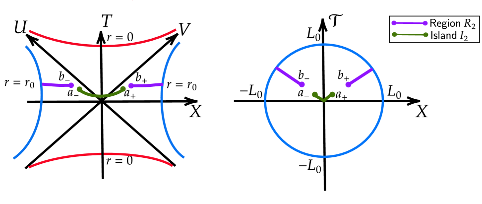
Figure 3: The schematic depicture of the region $R_{2}$ (magenta) in: two-boundary Lorentzian geometry (left) and its Euclidean version (right).

3.1 Without island

First apply the strategy of entanglement entropy calculation described in the previous section to the evolution of entanglement entropy (9)–(12) with conformal mapping (24) and Weyl transformation of the resulting curved UHP to the flat one. Here we study the entanglement entropy without island phase and explicitly choose the points $\mathbf{b}_{\pm}$ as

$$\mathbf{b}_{+}=\left(r_{b},t_{b}\right),\qquad\mathbf{b}_{-}=\left(r_{b},-t_{b}\right).$$ (31)

With this choice of points after some algebra one writes down the time-dependent entanglement entropy of $R_{2}$ as

$$S(R_{2})=\frac{c}{6}\log\left(\frac{4f(b)\cosh^{2}\kappa_{h}t_{b}}{\kappa^{2}_{h}\varepsilon^{2}}\right)+\frac{c}{6}\log\left(\frac{2\sinh^{2}\kappa_{h}(r_{*}(r_{0})-r_{*}(r_{b}))}{\cosh 2\kappa_{h}(r_{*}(r_{0})-r_{*}(r_{b}))+\cosh 2\kappa_{h}t_{b}}\right).$$ (32)

Note that in the limit $r_{0}\to\infty$ the second term of (32) tends to zero, so the entropy without boundary (the first term) is restored. At large times

$$t_{b}\gg t^{1}_{b},\qquad t^{1}_{b}\equiv r_{*}(r_{0})-r_{*}(r_{b}),$$ (33)

the entropy (32) saturates at the value

$$S(R_{2})=\frac{c}{6}\log\left(\frac{4f(b)\sinh^{2}\kappa_{h}(r_{*}(r_{0})-r_{*}(r_{b}))}{\kappa^{2}_{h}\varepsilon^{2}}\right).$$ (34)

The time dependence of the entanglement entropy (32) for different positions of the boundary $r_{0}$ and the comparison with the entanglement entropy for the case without boundaries (i.e. at $r_{0}\to\infty$) are shown in Fig. 4.

The time $t^{1}_{b}$ (33), until which the entanglement entropy (32) increases monotonically, depends on the location of the boundary $r_{0}$. For a sufficiently large $r_{0}$, the entropy (32) at some time $t_{b}<t^{1}_{b}$ starts to exceed the thermodynamic entropy of the black hole

$$S^{\text{therm}}_{BH}=\frac{2\pi r^{2}_{h}}{G},$$ (35)

which is equal to twice the Bekenstein-Hawking entropy. This leads to a violation of the unitarity of the evolution of the closed system “black hole + Hawking radiation”, which we interpret as an information paradox for a two-sided black hole with symmetric boundaries.

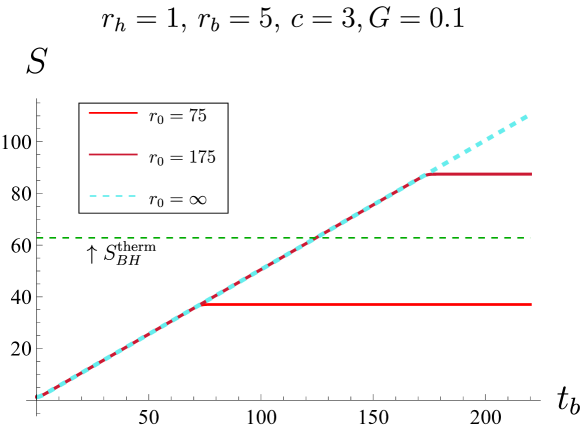
Figure 4: Time dependence of entanglement entropy without an island (32) for different boundary positions. The entanglement entropy initially increases monotonically the same way as in the case without boundaries ($r_{0}=\infty$), and approximately at the time (33) the entropy reaches saturation (34). The entropy saturation time increases with the increase of boundary location $r_{0}$. For a sufficiently far boundary, the entanglement entropy exceeds the thermodynamic entropy of a black hole $S^{\text{therm}}_{BH}$ (35) (dashed green line).

3.2 Blinking island solution

In the previous subsection it was shown that depending on the position of the boundary one can observe the exceed of entanglement entropy over black hole entropy. In this subsection we consider the entanglement entropy with a non-trivial island and examine whether this obstructs the excessive entanglement growth thus avoiding non-unitary dynamics i.e.

$$S(R_{2})(t_{b})<S^{\text{therm}}_{BH}$$ (36)

is to be satisfied at all points of time $t_{b}$.

Due to the symmetric choice of endpoints $\mathbf{b}_{\pm}$ (31) of the region $R_{2}$ and the symmetrical location of boundaries in both wedges, it follows that the endpoints $\mathbf{a}_{\pm}$ of island $I_{2}$ are also symmetric and are given as follows

$$\mathbf{a}_{+}=\left(r_{a},t_{a}\right),\qquad\mathbf{a}_{-}=\left(r_{a},-t_{a}\right),$$ (37)

where the point $\mathbf{a}_{+}$ ($\mathbf{a}_{-}$) is located in the right (left) wedge. The generalized entropy (28) with the symmetric island $I_{2}$ is

$$S_{\text{gen}}[I_{2},R_{2}]=S^{\text{wb}}_{I}(R_{2})+S^{\text{b}}_{I}(R_{2}),$$ (38)

where the first term $S^{\text{wb}}_{I}(R_{2})$ is independent of radial coordinate $r_{0}$ of boundary. In the limit $r_{0}\to\infty$ we are left only with this term corresponding to the generalized entropy for a two-sided black hole with regions extending to spacelike infinity Hashimoto:2020cas

$$S^{\text{wb}}_{I}(R_{2}) =\frac{2\pi r^{2}_{a}}{G}+\frac{c}{3}\log\left(\frac{4\sqrt{f(r_{a})f(r_{b})}\cosh\kappa_{h}t_{a}\cosh\kappa_{h}t_{b}}{\kappa^{2}_{h}\varepsilon^{2}}\right)$$ (39)

$$+\frac{c}{3}\log\left(\frac{\cosh\kappa_{h}(r_{*}(r_{a})-r_{*}(r_{b}))-\cosh\kappa_{h}(t_{a}-t_{b})}{\cosh\kappa_{h}(r_{*}(r_{a})-r_{*}(r_{b}))+\cosh\kappa_{h}(t_{a}+t_{b})}\right).$$

The second term of generalized entropy (38) is the contribution purely due to the boundary inclusion

$$S^{\text{b}}_{I}(R_{2})=\frac{c}{3}\log\left(\frac{\cosh\kappa_{h}(2r_{*}(r_{0})-r_{*}(r_{b})-r_{*}(r_{a}))+\cosh\kappa_{h}(t_{a}+t_{b})}{\cosh\kappa_{h}(2r_{*}(r_{0})-r_{*}(r_{b})-r_{*}(r_{a}))-\cosh\kappa_{h}(t_{a}-t_{b})}\right)$$ (40)

$$+\frac{c}{6}\log\left(\frac{4\sinh^{2}\kappa_{h}(r_{*}(r_{0})-r_{*}(r_{a}))\sinh^{2}\kappa_{h}(r_{*}(r_{0})-r_{*}(r_{b}))}{(\cosh 2\kappa_{h}(r_{*}(r_{0})-r_{*}(r_{a}))+\cosh 2\kappa_{h}t_{a})(\cosh 2\kappa_{h}(r_{*}(r_{0})-r_{*}(r_{b}))+\cosh 2\kappa_{h}t_{b})}\right).$$

In accordance with the prescription of the island formula (30), it is necessary to carry out extremization with respect to the radial and time coordinates $(r_{a},t_{a})$ of the island boundaries in (38), i.e. find the solutions of

$$\begin{cases}\partial_{r_{a}}S_{\text{gen}}[I_{2},R_{2}]\left(r_{a},t_{a},r_{b},t_{b},r_{0},r_{h},c,G\right)=0,\\ \partial_{t_{a}}S_{\text{gen}}[I_{2},R_{2}]\left(r_{a},t_{a},r_{b},t_{b},r_{0},r_{h},c,G\right)=0.\end{cases}$$ (41)

We consider solutions to the system (41) corresponding to the location of the island boundary $r_{a}$ near the horizon, i.e. $r_{a}=r_{h}+X$, $X/r_{h}\ll 1$. We also work within the framework of the condition $r_{b}\gg r_{h}$ (for the applicability of the s-wave approximation Hashimoto:2020cas ) and also assuming $cG\kappa^{2}_{h}\ll 1$.

For fixed parameters $(r_{b},r_{0},r_{h},c,G)$, the solution (or lack thereof) of the system (41) significantly depends on the time $t_{b}$. There are three different time $t_{b}$ regimes. Let us study each of them in detail.

• Early time regime:

  This time regime is determined by the following condition

  $$\cosh\kappa_{h}(t_{a}+t_{b}) \ll\cosh\kappa_{h}(2r_{*}(r_{0})-r_{*}(r_{a})-r_{*}(r_{b})),$$ (42)

  $$\cosh 2\kappa_{h}t_{a} \ll\cosh 2\kappa_{h}(r_{*}(r_{0})-r_{*}(r_{a})).$$

  If along with (42) the condition

  $$\cosh\kappa_{h}(t_{a}+t_{b})\gg\cosh\kappa_{h}(r_{*}(r_{b})-r_{*}(r_{a}))$$ (43)

  is also satisfied, then one can show that there is a non-trivial solution of the system (41)

  $$t_{a} \approx t_{b}-\frac{1}{2\kappa_{h}}\log\left[1-e^{2\kappa_{h}(t_{b}-r_{*}(r_{0})+r_{*}(r_{b}))}\right],$$ (44)

  $$r_{a} \approx r_{h}+\frac{c^{2}G^{2}e^{(r_{h}-r_{b})/r_{h}}}{144\pi^{2}r^{2}_{h}(r_{b}-r_{h})}-\frac{c^{2}G^{2}e^{(t_{b}+r_{h}-r_{0})/r_{h}}}{144\pi^{2}r^{2}_{h}(r_{0}-r_{h})}.$$ (45)

  In the limit $r_{0}\to\infty$ the solution (44), (45) corresponds to the solution for the case without boundaries Hashimoto:2020cas . From the condition that (44) is real, it follows that the solution in the early time regime exists only for

  $$t_{b}<t^{1}_{b},\qquad t^{1}_{b}=r_{*}(r_{0})-r_{*}(r_{b}).$$ (46)

  Recall that time $t^{1}_{b}$ approximately corresponds to the moment when the entanglement entropy without an island (32) reaches saturation.

• Intermediate time regime:

  This time regime is determined by the following condition

  $$\cosh\kappa_{h}(t_{a}+t_{b}) >\cosh\kappa_{h}(2r_{*}(r_{0})-r_{*}(r_{a})-r_{*}(r_{b})),$$ (47)

  $$\cosh 2\kappa_{h}t_{a} <\cosh 2\kappa_{h}(r_{*}(r_{0})-r_{*}(r_{a})).$$

  It can be shown that in the intermediate time regime there is no solution for an island near the horizon (see Appendix B for details).

• Late time regime:

  This time regime is determined by the following condition

  $$\cosh\kappa_{h}(t_{a}+t_{b}) \gg\cosh\kappa_{h}(2r_{*}(r_{0})-r_{*}(r_{a})-r_{*}(r_{b})),$$ (48)

  $$\cosh 2\kappa_{h}t_{a} \gg\cosh 2\kappa_{h}(r_{*}(r_{0})-r_{*}(r_{a})).$$

  Under this assumptions one can also explicitly calculate the approximate location of the horizon

  $$t_{a} \approx t_{b}-\frac{1}{2\kappa_{h}}\log\left[1-\frac{27\pi^{3}}{c^{3}G^{3}\kappa^{6}_{h}}e^{2\kappa_{h}(r_{*}(r_{0})+2r_{*}(r_{b})-t_{b})-3}\right],$$ (49)

  $$r_{a} \approx r_{h}+\frac{c^{2}G^{2}e^{(r_{h}-r_{b})/r_{h}}}{144\pi^{2}r^{2}_{h}(r_{b}-r_{h})}-\frac{12\pi r_{h}(r_{0}-r_{h})(r_{b}-r_{h})e^{\frac{r_{0}+r_{b}-2r_{h}-t_{b}}{r_{h}}}}{cG}.$$ (50)

  The formula (49) must be real-valued, so this implies the estimate for the existence of the island solution

  $$t_{b}>t^{2}_{b},\qquad t^{2}_{b}=r_{*}(r_{0})+2r_{*}(r_{b})-\frac{3}{2\kappa_{h}}\log\left(\frac{cG\kappa^{2}_{h}e}{3\pi}\right).$$ (51)

  In the limit $r_{0}\to\infty$ (51) one can see that $t^{2}_{b}\rightarrow\infty$, i.e. this means absence of the late time regime as it should be.

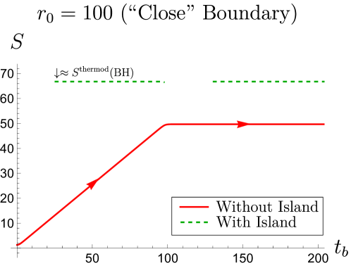
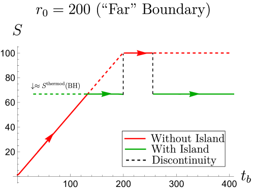
Figure 5: Time dependence of entanglement entropy taking into account nontrivial island configuration for a black hole with symmetric boundary for different boundary locations $r_{0}$.

The difference between the times $t^{2}_{b}$ and $t^{1}_{b}$ (see (51) and (46), respectively), that we call “blink time” $t_{\text{blink}}$, is equal to

$$t_{\text{blink}}\equiv t^{2}_{b}-t^{1}_{b}=3r_{*}(r_{b})-\frac{3}{2\kappa_{h}}\log\left(\frac{cG\kappa^{2}_{h}e}{3\pi}\right)$$ (52)

$$=6GM\left(\frac{r_{b}}{2GM}-\log\left[\frac{ce}{48\pi GM^{2}(r_{b}/2GM-1)}\right]\right).$$

As we mentioned earlier, calculations are carried out in the approximation $cG\kappa^{2}_{h}\ll 1$. From (52) this condition leads to the crucial relation

$$t^{2}_{b}>t^{1}_{b}.$$ (53)

It implies that during the time interval $t_{b}\in(t^{1}_{b},t^{2}_{b})$ island configuration near horizon does not exist. In the other words the general picture of island evolution is the following

• First the island appears and exists for some time and at $t_{b}=t^{1}_{b}$ disappears

• At time $t_{b}\in(t^{1}_{b},t^{2}_{b})$ island solution near horizon does not exist

• after the time $t^{2}_{b}$ it appears again and stays until the infinite time

Formally for a large number of fields $c$ it follows from (52) that $t^{2}_{b}<t^{1}_{b}$ for

$$c>\frac{3\pi}{G\kappa^{2}_{h}}e^{2\kappa_{h}r_{*}(r_{b})-1}.$$ (54)

So for such $c$ the island does not disappear for a finite period of time. However, we emphasize that (54) violates the approximation $cG\kappa^{2}_{h}\ll 1$ within which the calculations were carried out.

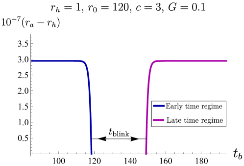
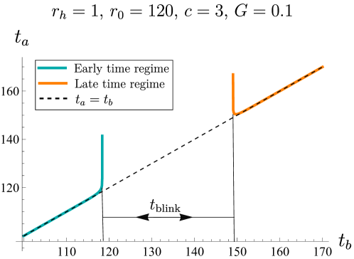
Figure 6: Dependence on the time $t_{b}$ of the island location $r_{a}$ (left)/time $t_{a}$ (right).

It also follows from the second line of (52) that for a fixed ratio $r_{b}/2GM=\text{fixed}$ and the fixed number of fields $c=\text{fixed}$, with an increase in the mass of the black hole $M$ the time difference $t_{\text{blink}}$ increases.

Thus the effect of the boundary in general is that it leads to the possibility of blink effect emergence – for a short time the island protecting us from the unitarity violation is switched off, thus leading to a short-time unitarity violation. Let us summarize in details the behaviour of entropy and the influence of this new effect of its dynamics

• As it was said in the previous subsection, for a boundary “close enough” to the event horizon, the entropy without an island reaches saturation before it exceeds the thermodynamic entropy of the black hole and the entropy with the island (see Fig.5 left). Thus, entanglement entropy without an island dominates throughout evolution, and non-unitary evolution does not take place, because condition (36) is satisfied for all times.

• For a “far enough” boundary, for which the entropy without an island at some point begins to exceed the thermodynamic entropy of a black hole, the situation is different. In this case, the island configuration, at least at some times, removes monotonous growth, which is consistent with unitary evolution. However, due to the disappearance of the island for a finite period of time $t_{\text{blink}}$ (52), the entanglement entropy jumps from a constant value of entropy with the island to a constant value of entropy without the island at saturation (34) (see Fig.5 right). Since the latter is greater than the thermodynamic entropy of a black hole, non-unitary evolution takes place, that is

  $$S(R_{2})(t_{b})>S^{\text{therm}}_{BH},\qquad t_{b}\in(t^{1}_{b},t^{2}_{b}).$$ (55)

• Thus, for a “close enough” boundary, an island is not needed for unitary evolution, and for a “far enough” boundary the fact of the island disappearing for a finite period of time $t_{\text{blink}}$ leads to non-unitary evolution.

• Now let us also discuss the behavior of extremization solutions, i.e. the radial and time coordinates $(r_{a},t_{a})$ of the island boundaries, depending on time $t_{b}$ (see Fig.6 demonstrating the numerical solution and (44), (45), (49), (50) for approximate analytical solutions). Most of the time during which the island exists, these solutions correspond to the “canonical” case without boundaries Hashimoto:2020cas . However, in the vicinity of the moments of time $t^{1}_{b}$ (time $t^{2}_{b}$) when the island disappears (appears), the radial coordinate $r_{a}$ decreases (increases) significantly, approaching the horizon $r_{h}$ (moving away from the horizon $r_{h}$), while the time coordinate $t_{a}$ increases (decreases) significantly.

3.3 Single-sided region

Let us finalize this section with consideration of the entanglement region $R_{r2}$ without entanglement dynamics in the double-boundary geometry. Let us choose this region  $R_{r2}$ being located only in the right wedge between spatial points $r_{b}$ and $r_{0}$ at some time $t_{b}$, see Fig.7 (left). The entanglement entropy of $R_{r2}$ in two-boundary geometry is just the constant and has no time dependence

$$S(R_{r2})=\frac{c}{6}\log\left(\frac{2\sqrt{f(r_{b})}\sinh\kappa_{h}(r_{*}(r_{0})-r_{*}(r_{b}))}{\kappa_{h}\varepsilon}\right).$$ (56)

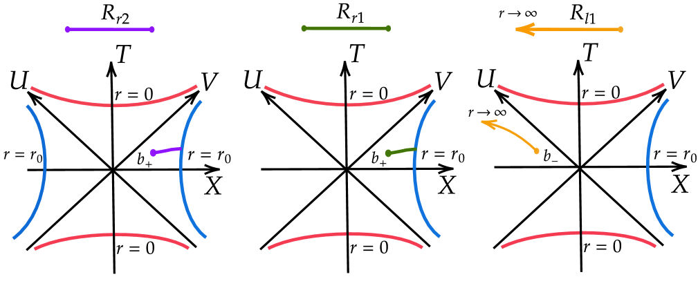
Figure 7: The schematic depicture of three types of one-wedge region. Left: region $R_{r2}$ (magenta) in double-boundary Lorentzian geometry. Center: region $R_{r1}$ (green) in single-boundary geometry similar to $R_{r2}$. Right: semi-infinite region $R_{l2}$ (orange) in left wedge of single-boundary geometry.

It is curious that a similar region $R_{r1}$ for a single-boundary geometry, see Fig.7 (center), which will be considered in the next section has the dynamics. Note that the entropy (56) infrared diverges when the boundary is removed, i.e. at $r_{0}\to\infty$.

4 Single-boundary geometry

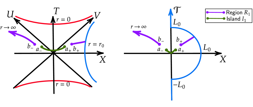
Figure 8: The schematic depicture of the region $R_{1}$ (magenta) in: two-boundary Lorentzian geometry (left) and its Euclidean version (right).

4.1 Without island

Let us start the study of entanglement entropy in single-boundary geometry introducing the analog of region $R_{2}$ (denote it $R_{1}$) and calculating the entanglement entropy $S(R_{1})$ for it. The region $R_{1}$ in the right wedge coincides with $R_{2}$ being restricted by the boundary location $r_{0}$ while in the left wedge which has no boundary it extends from point $\mathbf{b}_{-}$ to spatial infinity, see Fig. 8. As in the previous section we first calculate the entanglement entropy $S(R_{1})$ without inclusion of island mechanism

$$S(R_{1})=\frac{c}{6}\log\left(\frac{4f(r_{b})\cosh^{2}\kappa_{h}t_{b}}{\kappa^{2}_{h}\varepsilon^{2}}\right)+\frac{c}{6}\log\left(\frac{\cosh 2\kappa_{h}t_{b}+\cosh 2\kappa_{h}(r_{*}(r_{0})-r_{*}(r_{b}))}{\cosh^{2}\kappa_{h}t_{b}}\right)$$ (57)

$$+\frac{c}{6}\log\left(\frac{3}{8}\sin\left[\frac{2}{3}\arctan\frac{\cosh\kappa_{h}t_{b}}{\sinh\kappa_{h}(r_{*}(r_{0})-r_{*}(r_{b}))}\right]\sin\left[2\arctan\frac{\cosh\kappa_{h}t_{b}}{\sinh\kappa_{h}(r_{*}(r_{0})-r_{*}(r_{b}))}\right]\right).$$

Note that in the limit $r_{0}\to\infty$ the last two terms of (57) tend to zero, so the entropy without boundary (the first term) is restored.

The exclusion of one of the boundaries lead to the following picture of entanglement entropy dynamics (see Fig.9): first the system follows the linear growth regime $S(R_{1})\approx c\kappa_{h}t_{b}/3$ exactly as in the previous cases, then approximately at time $t^{1}_{b}=r_{*}(r_{0})-r_{*}(r_{b})$ the entropy (57) reduces to the twice weaker linear growth

$$S(R_{1})\simeq\frac{c\kappa_{h}t_{b}}{6}+\frac{c}{6}\log\left(\frac{3\sqrt{3}f(r_{b})}{2\kappa^{2}_{h}\varepsilon^{2}}\sinh\kappa_{h}(r_{*}(r_{0})-r_{*}(r_{b}))\right).$$ (58)

Note that for a similar region $R_{2}$, in the case of two symmetric boundaries, the entropy without an island (32) reaches a constant (34) at approximately the same time $t^{1}_{b}$. This difference can be interpreted so that in the case of one boundary, “equilibrium” occurs only in one wedge, while in the case of two boundaries – in both wedges.

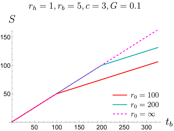
Figure 9: Time-dependence of entanglement entropy without the island term for the region $R_{1}$.

We also note one more important difference. For the case of two boundaries, the entropy without an island (32) at a sufficiently close location of the boundary $r_{0}$ relative to the horizon does not exceed the thermodynamic entropy of the black hole (35). While for the single-boundary case, the entropy without an island (57), due to the presence of monotonous growth at all times, exceeds the thermodynamic entropy (35) for any location of the boundary $r_{0}$. Thus, if there is no island configuration for such a region, then a non-unitary evolution takes place for all $r_{0}$.

4.2 Blinking island in single-boundary geometry

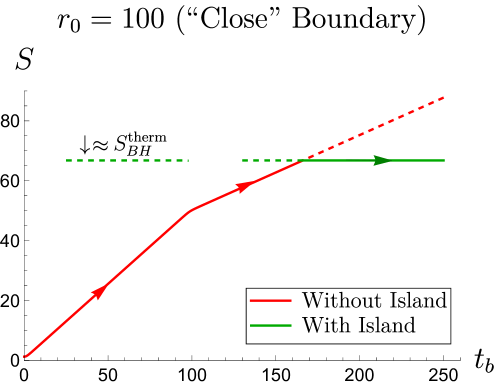
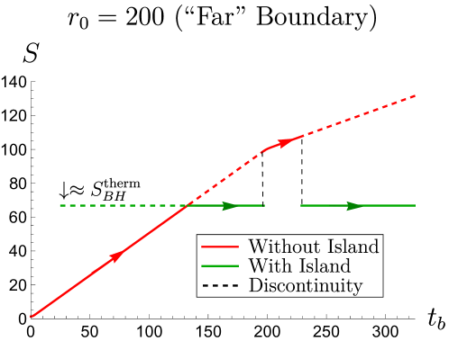
Figure 10: Time dependence of entanglement entropy taking into account nontrivial island configuration for a black hole with only one boundary for different boundary locations $r_{0}$.

So far in the previous section we observe that entanglement entropy in the geometry with asymmetric boundaries also lead us to the unbounded growth. In this subsection for region $R_{1}$ we consider the entanglement entropy with a non-trivial island $I_{1}$ and examine the possibility whether the island mechanism saves unitarity as well in the symmetry or one could observe “blinking island”. Again we assume that to avoid non-unitarity issues entanglement entropy should not exceed thermodynamic entropy of black hole for all times

$$S(R_{1})(t_{b})<S^{\text{therm}}_{BH}$$ (59)

where the thermodynamic entropy of a black hole is also given by the (35).

The presence of asymmetry between the right and left wedges indicates that the island configuration $I_{1}$ does not have to be symmetrical (with $\mathbf{b}_{\pm}$ given by (31)). Therefore, we select the island endpoints as

$$\mathbf{a}_{+}=\left(r_{a_{+}},t_{a_{+}}\right),\qquad\mathbf{a}_{-}=\left(r_{a_{-}},-t_{a_{-}}\right),$$ (60)

where the point $\mathbf{a}_{+}$ ($\mathbf{a}_{-}$) is located in the right (left) wedge. The generalized entropy (28) with the island $I_{1}$ is

$$S_{\text{gen}}[I_{1},R_{1}]=\frac{\pi r^{2}_{a_{+}}}{G}+\frac{\pi r^{2}_{a_{-}}}{G}+S_{\text{m}}(R_{1}\cup I_{1}),$$ (61)

where the matter entanglement entropy $S_{\text{m}}(R_{1}\cup I_{1})$ is calculated by applying the formulas (9)-(12) for region $R_{1}\cup I_{1}$. Unfortunately, in contrast to the case with two symmetrical boundaries, we could not find a readable analytical formula for $S_{\text{m}}(R_{1}\cup\leavevmode\nobreak\ I_{1})$ due to the difficult conformal transformation (25) for single-boundary geometry. All calculations for entanglement entropy with an island (i.e. numerical solution of extremization equation and use of island formula) in this section are performed numerically. As a result we find blinking island solution in single-boundary geometry (for region $R_{1}$). The time-dependence of entanglement entropy including the blinking island effect is presented in Fig.10 and it is qualitatively identical to the double-boundary geometry case (except the presence of linear growth with different coefficients at different time scales).

4.3 Single-sided regions

Exterior with boundary

Finally let us consider the dynamics of entanglement entropy for regions located in the single exterior. As we have shown in section 3.3, in double-boundary geometry region completely located in a single exterior is time-independent. In contrast to this we find that in the single-boundary geometry such type of region now has the dynamics. Again, to set up notation, we consider the geometry with the right exterior containing the boundary, and left is free of it. We denote the region in right exterior as $R_{r1}$ – this region is finite and bounded by some point $\mathbf{b}_{+}$ and the boundary, see Fig.7 (center).

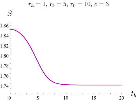
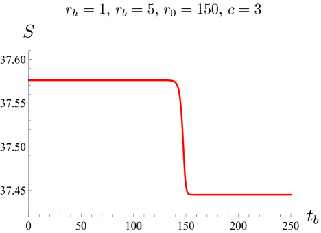
Figure 11: The time-dependence for entanglement entropy $S(R_{r1})$ for different reflecting boundaries values $r_{0}$.

Removing one of the boundaries leads to the dynamics of entanglement entropy. Explicitly, it is given by

$$S(R_{r1})= \,\frac{c}{12}\log\left(\frac{9f(r_{b})}{2\kappa^{2}_{h}\varepsilon^{2}}\left[\cosh 2\kappa_{h}t_{b}+\cosh 2\kappa_{h}(r_{*}(r_{0})-r_{*}(r_{b}))\right]\right)$$ (62)

$$+\frac{c}{6}\log\cos\left(\frac{\pi}{6}+\frac{2}{3}\arctan\frac{\cosh\kappa_{h}t_{b}}{\sinh\kappa_{h}(r_{*}(r_{0})-r_{*}(r_{b}))}\right),$$

and approximately at time $t^{1}_{b}=r_{*}(r_{0})-r_{*}(r_{b})$ it decrease to

$$S(R_{r1})\simeq\frac{c}{6}\log\left(\frac{2\sqrt{f(r_{b})}\sinh\kappa_{h}(r_{*}(r_{0})-r_{*}(r_{b}))}{\kappa_{h}\varepsilon}\right).$$ (63)

which coincides with (56). From Fig.11 one can see that the entanglement entropy is the constant until some time moment defined by boundary location just decreases to some constant value (for larger $r_{0}$ this transition is more sharp). If the boundary $r_{0}$ is relatively close to the horizon $r_{h}$ then the evolution already starts with the decrease.

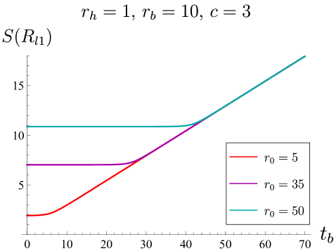
Figure 12: Time dependence of entanglement entropy (64) without an island for the region $R_{l1}$ located in the left wedge, for geometry with a boundary only in the right wedge at different values of $r_{0}$.

Exterior without boundary

By analogy let us consider the region $R_{l1}$ – region between spatial infinity and some points $\mathbf{b}_{-}$ in the left wedge, see Fig.7 (right). Again the entanglement entropy $S(R_{l1})$ is time-dependent and is given by

$$S(R_{l1})= \,\frac{c}{12}\log\left(\frac{9f(r_{b})}{2\kappa^{2}_{h}\varepsilon^{2}}\left[\cosh 2\kappa_{h}(r_{*}(r_{0})-r_{*}(r_{b}))+\cosh 2\kappa_{h}t_{b}\right]\right)$$ (64)

$$+\frac{c}{6}\log\sin\left(\frac{\pi}{3}\pm\frac{2}{3}\arctan\frac{\cosh\kappa_{h}t_{b}}{\sinh\kappa_{h}(r_{*}(r_{0})-r_{*}(r_{b}))}\right),$$

where the plus (minus) corresponds to $r_{0}>r_{b}$ ($r_{0}<r_{b}$). Remind that for double-boundary geometry or geometry without boundaries such a region has no dependence on time. Now if in the “entangled universe on the other side” one confined black hole in the box we will see the linear growth for $S(R_{l1})$ approximately at $t_{b}=|r_{*}(r_{0})-r_{*}(r_{b})|$

$$S(R_{l1})\simeq\frac{c\kappa_{h}t_{b}}{6}+\frac{c}{6}\log\left(\frac{3\sqrt{3}f(r_{b})}{4\kappa_{h}\varepsilon}\right).$$ (65)

Closer boundary “on the other side” is located to the horizon – faster the growth will start “on this side”. For this case one can find the asymmetric insland solution numerically (for simplicity we do not present them).

5 Discussion and main results

Let us briefly summarize our results. We deform the geometry of eternal black hole locating boundaries at some distance from the horizon. We consider two situations, double-boundary geometry, when we place boundaries symmetrical in each exterior, and single-boundary geometry, when only one exterior contains boundary. For these types of geometries we find that

• In contrast to geometry without any boundary which has the unlimited entanglement entropy growth (when entangling region is semi-infinite and located in both exteriors), in double-boundary geometry the growth stops after some time proportional to the boundary location. When location of the boundary tends to infinity, $r_{0}\rightarrow\infty$, this time also becomes infinite. In this way for some $r_{0}$ we do not have information paradox at all – the entropy never exceeds thermodynamical entropy. In some sense this resembles the situation with calculation of heat capacity – without boundaries the capacity of Schwarzschild solution is negative which indicates the instability. However, if we include the boundaries then the capacity becomes positive for some black hole masses York:1986it .

• Examining asymmetric geometry where the boundary is present in only one exterior (i.e. total state corresponds to two entangled states, one with the boundary and one without it), we observe that entanglement entropy becomes dynamical for entanglement regions that are completely contained within the single exterior. Remind that when left and right exteriors are symmetric in the same situation no dynamics in the entanglement entropy could be observed.

Appendix A Conformal map from single-boundary geometry to UHP

In this subsection, we prove that the conformal transformation from the Euclidean geometry of a two-sided black hole with a boundary in only one wedge (see Fig.13.A), associated with the complex coordinate $w=X+i{\cal T}$ (22), to the upper half-plane is given by (25).

As discussed in the setup, the domain under consideration in Euclidean single-boundary geometry in the plane $({\cal T},X)$ corresponds to the union of left half-plane $X<0$ (denote it $\Omega_{1}$) and the interior of a semi-disk in the right half-plane $X>0$ with the radius $L_{0}=e^{\kappa_{h}r_{*}(r_{0})}/\kappa_{h}$ (denote it $\Omega_{2}$). So, the domain in question of the complex plane $\omega$ is $\Omega=\Omega_{1}\cup\Omega_{2}$. Let us express the complex variable $w$ in exponential form

$$w=\rho e^{i\theta}.$$ (66)

We present the conformal map (25) from $\Omega$ to UHP as a composition of several simple conformal maps: $\Omega\to\Sigma\to H\to\text{UHP}$, see Fig.13.

• Transform $\Omega\to\Sigma$ by inversion with multiplication by constant

  $$\sigma=\frac{iL_{0}}{w},\quad\sigma=\varrho e^{i\varphi}\,\,\,\Rightarrow\,\,\,\varrho=\frac{L_{0}}{\rho},\,\,\varphi=\frac{\pi}{2}-\theta.$$ (67)

  The domain $\Omega_{1}=\{\rho\in[0,+\infty),\,\,\theta\in\left[\pi/2,3\pi/2\right]\}$ under conformal map (67) transforms to the lower half-plane $\Sigma_{1}=\{\varrho\in[0,+\infty)$, $\varphi\in\left[-\pi,0\right]\}$.

  The domain $\Omega_{2}=\{\rho\in[0,L_{0}],\,\,\theta\in\left[-\pi/2,\pi/2\right]\}$ under conformal map (67) transforms to the exterior of unit semi-disk in the upper half-plane
  $\Sigma_{2}=\{\varrho\in[1,+\infty)$, $\varphi\in\left[0,\pi\right]\}$.

  The resulting domain of the complex plane $\sigma$ is $\Sigma=\Sigma_{1}\cup\Sigma_{2}$ (see Fig.13.B).

• Transform $\Sigma\to H$ by fractional-linear transformation

  $$\eta=\frac{\sigma-1}{\sigma+1},\,\,\,\eta=\xi e^{i\lambda}\Rightarrow\xi=\sqrt{\frac{1+\varrho^{2}-2\varrho\cos\varphi}{1+\varrho^{2}+2\varrho\cos\varphi}},\,\,\,\lambda=\arctan\left(\frac{2\varrho\sin\varphi}{\varrho^{2}-1}\right)+k\pi.$$ (68)

  where $k=0$ ($k=1$) is for $\varrho>1$ ($\varrho<1$).

  The domain $\Sigma_{1}$ under conformal map (68) transforms to the lower half-plane $H_{1}=\{\xi\in[0,+\infty)$, $\lambda\in\left[-\pi,0\right]\}$.

  The domain $\Sigma_{2}$ under conformal map (68) transforms to the first quadrant $H_{2}=\{\xi\in[0,+\infty)$, $\lambda\in\left[0,\pi/2\right]\}$.

  The resulting domain of the complex plane $\eta$ is $H=H_{1}\cup H_{2}$ (see Fig.13.C).

  

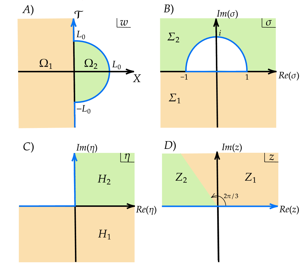
  Figure 13: A sequence of conformal transformations from the union of the left half-plane and the interior of the unit disk in the right half-plane (A) to the upper half-plane (D).

• Transform $H\to\text{UHP}$ by

  $$z=e^{2\pi i/3}\eta^{2/3},\,\,\,z=\chi e^{i\psi}\quad\Rightarrow\quad\chi=\xi^{2/3},\,\,\,\psi=\frac{2}{3}\left(\lambda+\pi\right),$$ (69)

  where we choose the root of the third degree of a complex number $\zeta=x\,e^{iy}$ that corresponds to the principal branch $\zeta^{1/3}=x^{1/3}e^{iy/3}$.

  The domain $H_{1}$ under conformal map (69) transforms to the sector in the upper half-plane $Z_{1}=\{\chi\in[0,+\infty)$, $\psi\in\left[0,2\pi/3\right]\}$.

  The domain $H_{2}$ under conformal map (69) transforms to the sector in the upper half-plane $Z_{2}=\{\chi\in[0,+\infty)$, $\psi\in\left[2\pi/3,\pi\right]\}$.

  The resulting domain of the complex plane $z$ is $\text{UHP}=Z_{1}\cup Z_{2}$ (see Fig.13.D).

Combining the above conformal maps (67)–(69), one can obtain the conformal transformation $\Omega\to\text{UHP}$ given by (25).

Appendix B The absence of island in the intermediate time regime

To obtain the entanglement entropy, it is necessary to carry out the extremization of the generalized entropy with respect to coordinates $(r_{a},t_{a})$ of the island configuration endpoints $\mathbf{a}_{\pm}$, see formula (41) and discussions about it.

In this appendix, we explicitly show that for the case with symmetrical boundaries in both exteriors, considered in Section 3, an island near horizon, i.e. with $r_{a}=r_{h}+X$, $X/r_{h}\ll 1$, does not exist in the intermediate time regime (47) for $cG\kappa^{2}_{h}\ll 1$.

For the convenience of analytical calculations, instead of extremization by $(r_{a},t_{a})$, we consider extremization by $\left(r_{*}(r_{a}),t_{a}\right)$. More precisely, we show that under the above conditions, the following system of equations

$$\begin{cases}\displaystyle\frac{\partial S_{\text{gen}}[I_{2},R_{2}]}{\partial t_{a}}=0,\\ \displaystyle\frac{\partial S_{\text{gen}}[I_{2},R_{2}]}{\partial r_{*}(r_{a})}-\displaystyle\frac{\partial S_{\text{gen}}[I_{2},R_{2}]}{\partial t_{a}}=0.\end{cases}$$ (70)

where $S_{\text{gen}}[I_{2},R_{2}]$ is given by (37), does not have the required solution near horizon.

We perform calculations under the following natural assumptions

$$r_{*}(r_{a})<0,\qquad e^{2\kappa_{h}r_{*}(r_{a})}\ll 1,\qquad\kappa_{h}(r_{*}(r_{0})-r_{*}(r_{a}))\gg 1,$$ (71)

$$\kappa_{h}t_{a,b}\gg 1,\qquad 2r_{*}(r_{0})-r_{*}(r_{a})-r_{*}(r_{b})\gg|t_{a}-t_{b}|.$$

Let us denote $S_{\text{gen}}[I_{2},R_{2}]={\cal S}$. Under the conditions (71) the explicit expression for the time derivative is

$$\frac{\partial{\cal S}}{\partial t_{a}}\simeq\frac{c\kappa_{h}}{3}\Big{(}\frac{2\sinh\kappa_{h}(t_{a}-t_{b})}{e^{\kappa_{h}(2r_{*}(r_{0})-r_{*}(r_{a})-r_{*}(r_{b}))}}-\frac{e^{\kappa_{h}(t_{a}+t_{b})}}{e^{\kappa_{h}(r_{*}(r_{b})-r_{*}(r_{a}))}+e^{\kappa_{h}(t_{a}+t_{b})}}-\frac{e^{2\kappa_{h}t_{a}}}{e^{2\kappa_{h}(r_{*}(r_{0})-r_{*}(r_{a}))}+e^{2\kappa_{h}t_{a}}}$$ (72)

$$-\frac{2\sinh\kappa_{h}(t_{a}-t_{b})}{e^{\kappa_{h}(r_{*}(r_{b})-r_{*}(r_{a}))}-2\cosh\kappa_{h}(t_{a}-t_{b})}+\frac{e^{\kappa_{h}(t_{a}+t_{b})}}{e^{\kappa_{h}(2r_{*}(r_{0})-r_{*}(r_{b})-r_{*}(r_{a}))}+e^{\kappa_{h}(t_{a}+t_{b})}}+1\Big{)},$$

and an explicit expression for the difference of the derivatives is given by

$$\frac{\partial{\cal S}}{\partial r_{*}(r_{a})}-\frac{\partial{\cal S}}{\partial t_{a}}\simeq \frac{2\pi e^{2\kappa_{h}r_{*}(r_{a})-1}}{G\kappa_{h}}+\frac{c\kappa_{h}}{3}\Big{(}1-\frac{e^{\kappa_{h}(r_{*}(r_{b})-r_{*}(r_{a}))}-2\sinh\kappa_{h}(t_{a}-t_{b})}{e^{\kappa_{h}(r_{*}(r_{b})-r_{*}(r_{a}))}-2\cosh\kappa_{h}(t_{a}-t_{b})}$$ (73)

$$-2e^{2\kappa_{h}r_{*}(r_{a})-1}+2e^{-\kappa_{h}(2r_{*}(r_{0})-r_{*}(r_{a})-r_{*}(r_{b})+t_{a}-t_{b})}\Big{)}.$$

Let us simplify the time derivative (72) in accordance with the intermediate time regime (47), considering that condition (43) is satisfied. Then

$$\frac{\partial{\cal S}}{\partial t_{a}}\simeq\frac{c\kappa_{h}}{3}\Big{(}1+\gamma-\frac{2\sinh\kappa_{h}(t_{a}-t_{b})}{e^{\kappa_{h}(r_{*}(r_{b})-r_{*}(r_{a}))}-2\cosh\kappa_{h}(t_{a}-t_{b})}\Big{)},$$ (74)

where

$$\gamma= -\frac{e^{\kappa_{h}(2r_{*}(r_{0})-r_{*}(r_{a})-r_{*}(r_{b}))}}{e^{\kappa_{h}(t_{a}+t_{b})}}-\frac{e^{2\kappa_{h}t_{a}}}{e^{2\kappa_{h}(r_{*}(r_{0})-r_{*}(r_{a}))}}$$ (75)

$$+\frac{e^{\kappa_{h}(r_{*}(r_{b})-r_{*}(r_{a}))}}{e^{\kappa_{h}(t_{a}+t_{b})}}+\frac{2\sinh\kappa_{h}(t_{a}-t_{b})}{e^{\kappa_{h}(2r_{*}(r_{0})-r_{*}(r_{a})-r_{*}(r_{b}))}}\ll 1.$$

Equating the expression on the right-hand side of (74) to zero, we obtain

$$e^{\kappa_{h}(t_{a}-t_{b})}=\frac{e^{\kappa_{h}(r_{*}(r_{b})-r_{*}(r_{a}))}(1+\gamma)\pm\sqrt{e^{2\kappa_{h}(r_{*}(r_{b})-r_{*}(r_{a}))}(1+\gamma)^{2}-4\gamma(2+\gamma)}}{2(2+\gamma)}.$$ (76)

We expand these expressions with respect to small $\gamma\ll 1$

$$e^{\kappa_{h}(t_{a}-t_{b})}\simeq\left\{\begin{array}[]{cc}\left(1+\gamma/2\right)e^{\kappa_{h}(r_{*}(r_{b})-r_{*}(r_{a}))}/2,\\ \gamma\,e^{-\kappa_{h}(r_{*}(r_{b})-r_{*}(r_{a}))},\end{array}\right.$$ (77)

where the top (bottom) row corresponds to the plus (minus) in (76).

Substituting the top row from (77) to the difference (73), we get

$$\frac{\partial{\cal S}}{\partial r_{*}(r_{a})}-\frac{\partial{\cal S}}{\partial t_{a}}\Big{|}_{\text{top row}}\simeq 2c\kappa_{h}e^{2\kappa_{h}r_{*}(r_{a})-1}\left[\frac{\pi}{cG\kappa^{2}_{h}}-\frac{1}{3}\left(1+4e^{1-2\kappa_{h}r_{*}(r_{b})}+\ldots\right)\right],$$ (78)

where the ellipsis denotes terms are even smaller than those indicated in parentheses. Note that $4e^{1-2\kappa_{h}r_{*}(r_{b})}\ll 1$ due to $r_{h}\ll r_{b}$. So, since the calculations are carried out in the approximation $cG\kappa^{2}_{h}\ll 1$, it turns out that the first term in (78), which is positive, is much larger than the negative second term. Therefore, the difference (78) is positive and does not equal to zero.

Substituting the bottom row from (77) to the difference (73), we get

$$\frac{\partial{\cal S}}{\partial r_{*}(r_{a})}-\frac{\partial{\cal S}}{\partial t_{a}}\Big{|}_{\text{b. row}}\simeq 2c\kappa_{h}e^{2\kappa_{h}r_{*}(r_{a})-1}\left[\frac{\pi}{cG\kappa^{2}_{h}}+\frac{1}{3}\left(e^{1-2\kappa_{h}r_{*}(r_{a})}-1+\ldots\right)\right].$$ (79)

Note that $e^{1-2\kappa_{h}r_{*}(r_{a})}>1$ due to $r_{*}(r_{a})<0$. So, it is clear that the expression (79) is positive and essentially different from zero.

Thus, it is shown that in the intermediate time regime under natural conditions there is no nontrivial island configuration such that its endpoints are near the horizon.

References

- (1) S. W. Hawking, “Particle Creation by Black Holes,” Commun. Math. Phys. 43, 199-220 (1975)
- (2) S. W. Hawking, “Breakdown of Predictability in Gravitational Collapse,” Phys. Rev. D 14 (1976), 2460-2473
- (3) D. N. Page, “Information in black hole radiation,” Phys. Rev. Lett. 71 (1993), 3743-3746 [arXiv:hep-th/9306083 [hep-th]].
- (4) D. N. Page, “Time Dependence of Hawking Radiation Entropy,” JCAP 09 (2013), 028 [arXiv:1301.4995 [hep-th]].
- (5) G. Penington, “Entanglement Wedge Reconstruction and the Information Paradox,” JHEP 09 (2020), 002 [arXiv:1905.08255 [hep-th]].
- (6) A. Almheiri, N. Engelhardt, D. Marolf and H. Maxfield, “The entropy of bulk quantum fields and the entanglement wedge of an evaporating black hole,” JHEP 12 (2019), 063 [arXiv:1905.08762 [hep-th]].
- (7) A. Almheiri, R. Mahajan, J. Maldacena and Y. Zhao, “The Page curve of Hawking radiation from semiclassical geometry,” JHEP 03 (2020), 149 [arXiv:1908.10996 [hep-th]].
- (8) G. Penington, S. H. Shenker, D. Stanford and Z. Yang, “Replica wormholes and the black hole interior,” JHEP 03 (2022), 205 [arXiv:1911.11977 [hep-th]].
- (9) A. Almheiri, T. Hartman, J. Maldacena, E. Shaghoulian and A. Tajdini, “Replica Wormholes and the Entropy of Hawking Radiation,” JHEP 05 (2020), 013 [arXiv:1911.12333 [hep-th]].
- (10) A. Almheiri, R. Mahajan and J. Maldacena, “Islands outside the horizon,” [arXiv:1910.11077 [hep-th]].
- (11) H. Z. Chen, R. C. Myers, D. Neuenfeld, I. A. Reyes and J. Sandor, “Quantum Extremal Islands Made Easy, Part I: Entanglement on the Brane,” JHEP 10 (2020), 166 [arXiv:2006.04851 [hep-th]].
- (12) A. Almheiri, T. Hartman, J. Maldacena, E. Shaghoulian and A. Tajdini, “The entropy of Hawking radiation,” Rev. Mod. Phys. 93 (2021) no.3, 035002 [arXiv:2006.06872 [hep-th]].
- (13) H. Z. Chen, R. C. Myers, D. Neuenfeld, I. A. Reyes and J. Sandor, “Quantum Extremal Islands Made Easy, Part II: Black Holes on the Brane,” JHEP 12 (2020), 025 [arXiv:2010.00018 [hep-th]].
- (14) M. Rozali, J. Sully, M. Van Raamsdonk, C. Waddell and D. Wakeham, “Information radiation in BCFT models of black holes,” JHEP 05 (2020), 004 [arXiv:1910.12836 [hep-th]].
- (15) J. Sully, M. Van Raamsdonk and D. Wakeham, “BCFT entanglement entropy at large central charge and the black hole interior,” JHEP 03 (2021), 167 [arXiv:2004.13088 [hep-th]].
- (16) H. Geng, S. Lüst, R. K. Mishra and D. Wakeham, “Holographic BCFTs and Communicating Black Holes,” jhep 08 (2021), 003 [arXiv:2104.07039 [hep-th]].
- (17) D. S. Ageev, “Shaping contours of entanglement islands in BCFT,” JHEP 03 (2022), 033 [arXiv:2107.09083 [hep-th]].
- (18) H. Geng, A. Karch, C. Perez-Pardavila, S. Raju, L. Randall, M. Riojas and S. Shashi, “Entanglement phase structure of a holographic BCFT in a black hole background,” JHEP 05 (2022), 153 [arXiv:2112.09132 [hep-th]].
- (19) K. Suzuki and T. Takayanagi, “BCFT and Islands in two dimensions,” JHEP 06 (2022), 095 [arXiv:2202.08462 [hep-th]].
- (20) Q. L. Hu, D. Li, R. X. Miao and Y. Q. Zeng, “AdS/BCFT and Island for curvature-squared gravity,” JHEP 09 (2022), 037 [arXiv:2202.03304 [hep-th]].
- (21) P. J. Hu, D. Li and R. X. Miao, “Island on codimension-two branes in AdS/dCFT,” JHEP 11 (2022), 008 [arXiv:2208.11982 [hep-th]].
- (22) J. Basak Kumar, D. Basu, V. Malvimat, H. Parihar and G. Sengupta, “Reflected entropy and entanglement negativity for holographic moving mirrors,” JHEP 09 (2022), 089 [arXiv:2204.06015 [hep-th]].
- (23) M. Afrasiar, J. Kumar Basak, A. Chandra and G. Sengupta, “Islands for entanglement negativity in communicating black holes,” Phys. Rev. D 108 (2023) no.6, 066013 [arXiv:2205.07903 [hep-th]].
- (24) H. Geng, L. Randall and E. Swanson, “BCFT in a black hole background: an analytical holographic model,” JHEP 12 (2022), 056 [arXiv:2209.02074 [hep-th]].
- (25) P. C. W. Davies and S. A. Fulling, “Radiation from a moving mirror in two-dimensional space-time conformal anomaly,” Proc. Roy. Soc. Lond. A 348 (1976), 393-414
- (26) M. R. R. Good, K. Yelshibekov and Y. C. Ong, “On Horizonless Temperature with an Accelerating Mirror,” JHEP 03 (2017), 013 [arXiv:1611.00809 [gr-qc]].
- (27) P. Chen and D. h. Yeom, “Entropy evolution of moving mirrors and the information loss problem,” Phys. Rev. D 96 (2017) no.2, 025016 [arXiv:1704.08613 [hep-th]].
- (28) M. R. R. Good, E. V. Linder and F. Wilczek, “Moving mirror model for quasithermal radiation fields,” Phys. Rev. D 101 (2020) no.2, 025012 [arXiv:1909.01129 [gr-qc]].
- (29) I. Akal, Y. Kusuki, N. Shiba, T. Takayanagi and Z. Wei, “Entanglement Entropy in a Holographic Moving Mirror and the Page Curve,” Phys. Rev. Lett. 126 (2021) no.6, 061604 [arXiv:2011.12005 [hep-th]].
- (30) K. Kawabata, T. Nishioka, Y. Okuyama and K. Watanabe, “Probing Hawking radiation through capacity of entanglement,” JHEP 05, 062 (2021) [arXiv:2102.02425 [hep-th]].
- (31) I. A. Reyes, “Moving Mirrors, Page Curves, and Bulk Entropies in AdS2,” Phys. Rev. Lett. 127, no.5, 051602 (2021) [arXiv:2103.01230 [hep-th]].
- (32) I. Akal, Y. Kusuki, N. Shiba, T. Takayanagi and Z. Wei, “Holographic moving mirrors,” Class. Quant. Grav. 38, no.22, 224001 (2021) [arXiv:2106.11179 [hep-th]].
- (33) D. Fernández-Silvestre, J. Foo and M. R. R. Good, “On the duality of Schwarzschild–de Sitter spacetime and moving mirror,” Class. Quant. Grav. 39, no.5, 055006 (2022) [arXiv:2109.04147 [gr-qc]].
- (34) I. Akal, T. Kawamoto, S. M. Ruan, T. Takayanagi and Z. Wei, “Zoo of holographic moving mirrors,” JHEP 08, 296 (2022) [arXiv:2205.02663 [hep-th]].
- (35) K. Hashimoto, N. Iizuka and Y. Matsuo, “Islands in Schwarzschild black holes,” JHEP 06 (2020), 085 [arXiv:2004.05863 [hep-th]].
- (36) M. Alishahiha, A. Faraji Astaneh and A. Naseh, “Island in the presence of higher derivative terms,” JHEP 02, 035 (2021) [arXiv:2005.08715 [hep-th]].
- (37) Y. Ling, Y. Liu and Z. Y. Xian, “Island in Charged Black Holes,” JHEP 03, 251 (2021) [arXiv:2010.00037 [hep-th]].
- (38) Y. Matsuo, “Islands and stretched horizon,” JHEP 07, 051 (2021) [arXiv:2011.08814 [hep-th]].
- (39) G. K. Karananas, A. Kehagias and J. Taskas, “Islands in linear dilaton black holes,” JHEP 03, 253 (2021) [arXiv:2101.00024 [hep-th]].
- (40) X. Wang, R. Li and J. Wang, “Islands and Page curves of Reissner-Nordström black holes,” JHEP 04, 103 (2021) [arXiv:2101.06867 [hep-th]].
- (41) W. Kim and M. Nam, “Entanglement entropy of asymptotically flat non-extremal and extremal black holes with an island,” Eur. Phys. J. C 81, no.10, 869 (2021) [arXiv:2103.16163 [hep-th]].
- (42) Y. Lu and J. Lin, “Islands in Kaluza–Klein black holes,” Eur. Phys. J. C 82, no.2, 132 (2022) [arXiv:2106.07845 [hep-th]].
- (43) M. H. Yu and X. H. Ge, “Islands and Page curves in charged dilaton black holes,” Eur. Phys. J. C 82, no.1, 14 (2022) [arXiv:2107.03031 [hep-th]].
- (44) B. Ahn, S. E. Bak, H. S. Jeong, K. Y. Kim and Y. W. Sun, “Islands in charged linear dilaton black holes,” Phys. Rev. D 105, no.4, 046012 (2022) [arXiv:2107.07444 [hep-th]].
- (45) N. H. Cao, “Entanglement entropy and Page curve of black holes with island in massive gravity,” Eur. Phys. J. C 82, no.4, 381 (2022) [arXiv:2108.10144 [hep-th]].
- (46) S. Azarnia, R. Fareghbal, A. Naseh and H. Zolfi, “Islands in flat-space cosmology,” Phys. Rev. D 104, no.12, 126017 (2021) [arXiv:2109.04795 [hep-th]].
- (47) I. Aref’eva and I. Volovich, “A note on islands in Schwarzschild black holes,” Teor. Mat. Fiz. 214, no.3, 500-516 (2023) [arXiv:2110.04233 [hep-th]].
- (48) S. He, Y. Sun, L. Zhao and Y. X. Zhang, “The universality of islands outside the horizon,” JHEP 05, 047 (2022) [arXiv:2110.07598 [hep-th]].
- (49) M. H. Yu, C. Y. Lu, X. H. Ge and S. J. Sin, “Island, Page curve, and superradiance of rotating BTZ black holes,” Phys. Rev. D 105, no.6, 066009 (2022) [arXiv:2112.14361 [hep-th]].
- (50) I. Y. Aref’eva, T. A. Rusalev and I. V. Volovich, “Entanglement entropy of a near-extremal black hole,” Teor. Mat. Fiz. 212, no.3, 457-477 (2022) [arXiv:2202.10259 [hep-th]].
- (51) W. C. Gan, D. H. Du and F. W. Shu, “Island and Page curve for one-sided asymptotically flat black hole,” JHEP 07, 020 (2022) [arXiv:2203.06310 [hep-th]].
- (52) S. Azarnia and R. Fareghbal, “Islands in Kerr–de Sitter spacetime and their flat limit,” Phys. Rev. D 106, no.2, 026012 (2022) [arXiv:2204.08488 [hep-th]].
- (53) A. Anand, “Page curve and island in EGB gravity,” Nucl. Phys. B 993, 116284 (2023) [arXiv:2205.13785 [hep-th]].
- (54) D. S. Ageev and I. Y. Aref’eva, “Thermal density matrix breaks down the Page curve,” Eur. Phys. J. Plus 137, no.10, 1188 (2022) [arXiv:2206.04094 [hep-th]].
- (55) D. S. Ageev, I. Y. Aref’eva, A. I. Belokon, A. V. Ermakov, V. V. Pushkarev and T. A. Rusalev, “Infrared regularization and finite size dynamics of entanglement entropy in Schwarzschild black hole,” Phys. Rev. D 108, no.4, 046005 (2023) [arXiv:2209.00036 [hep-th]].
- (56) J. W. York, Jr., “Black hole thermodynamics and the Euclidean Einstein action,” Phys. Rev. D 33 (1986), 2092-2099
- (57) D. J. Gross, M. J. Perry and L. G. Yaffe, “Instability of Flat Space at Finite Temperature,” Phys. Rev. D 25, 330-355 (1982)
- (58) Y. K. Yazdi, “Zero Modes and Entanglement Entropy,” JHEP 04, 140 (2017) [arXiv:1608.04744 [hep-th]].
- (59) G. W. Gibbons and S. W. Hawking, “Cosmological Event Horizons, Thermodynamics, and Particle Creation,” Phys. Rev. D 15, 2738-2751 (1977)
- (60) H. Saida, “To what extent is the entropy-area law universal?: Multi-horizon and multi-temperature spacetime may break the entropy-area law,” Prog. Theor. Phys. 122, 1515-1552 (2010) [arXiv:0910.2510 [gr-qc]].
- (61) M. S. Ma, R. Zhao and Y. Q. Ma, “Thermodynamic stability of black holes surrounded by quintessence,” Gen. Rel. Grav. 49, no.6, 79 (2017) [arXiv:1606.06070 [gr-qc]].
- (62) J. Maldacena and L. Susskind, “Cool horizons for entangled black holes,” Fortsch. Phys. 61 (2013), 781-811 [arXiv:1306.0533 [hep-th]].
- (63) P. Calabrese and J. L. Cardy, “Entanglement entropy and quantum field theory,” J. Stat. Mech. 0406 (2004), P06002 [arXiv:hep-th/0405152 [hep-th]].
- (64) P. Calabrese and J. Cardy, “Entanglement entropy and conformal field theory,” J. Phys. A 42 (2009), 504005 [arXiv:0905.4013 [cond-mat.stat-mech]].
- (65) J. L. Cardy, “Conformal Invariance and Surface Critical Behavior,” Nucl. Phys. B 240 (1984), 514-532
- (66) J. L. Cardy, “Effect of Boundary Conditions on the Operator Content of Two-Dimensional Conformally Invariant Theories,” Nucl. Phys. B 275 (1986), 200-218
- (67) J. L. Cardy, “Boundary Conditions, Fusion Rules and the Verlinde Formula,” Nucl. Phys. B 324 (1989), 581-596
- (68) M. Mintchev and E. Tonni, “Modular Hamiltonians for the massless Dirac field in the presence of a boundary,” JHEP 03 (2021), 204 [arXiv:2012.00703 [hep-th]].
- (69) F. Rottoli, S. Murciano, E. Tonni and P. Calabrese, “Entanglement and negativity Hamiltonians for the massless Dirac field on the half line,” J. Stat. Mech. 2301 (2023), 013103 [arXiv:2210.12109 [cond-mat.stat-mech]].
- (70) J. Kruthoff, R. Mahajan and C. Murdia, “Free fermion entanglement with a semitransparent interface: the effect of graybody factors on entanglement islands,” SciPost Phys. 11 (2021), 063 [arXiv:2106.10287 [hep-th]].