Learning Reionization History from Quasars with Simulation-Based Inference

Abstract

Understanding the entire history of the ionization state of the intergalactic medium (IGM) is at the frontier of astrophysics and cosmology. A promising method to achieve this is by extracting the damping wing signal from the neutral IGM. As hundreds of redshift $z>6$ quasars are observed, we anticipate determining the detailed time evolution of the ionization fraction with unprecedented fidelity. However, traditional approaches to parameter inference are not sufficiently accurate.

We assess the performance of a simulation-based inference (SBI) method to infer the neutral fraction of the universe from quasar spectra. The SBI method adeptly exploits the shape information of the damping wing, enabling precise estimations of the neutral fraction ${\left<x_{\rm HI}\right>_{\rm v}}$ and the wing position $w_{p}$. Importantly, the SBI framework successfully breaks the degeneracy between these two parameters, offering unbiased estimates of both. This makes the SBI superior to the traditional method using a pseudo-likelihood function. We anticipate that SBI will be essential to determine robustly the ionization history of the Universe through joint inference from the hundreds of high-$z$ spectra we will observe.

1 Introduction

Understanding the evolution of the neutral fraction of the universe is a central topic in the study of cosmic reionization. Up to now, the most successful and well-known constraint has been from analyzing the Thompson scattering signal in the Cosmic Microwave Background (CMB)[1, 2, 9, 27]. However, due to its integrated effect in the CMB, constraining the detailed time evolution of the cosmic neutral fraction is challenging. Another approach is to analyze the effect of the neutral intergalactic medium (IGM) on spectra from quasars directly living in the epoch of reionization (Fig. 1). With hundreds of high-redshift quasars discovered and followed-up spectroscopically [11, 3, 25], this method could potentially surpass the CMB method in the near future, if the information can be extracted reliably.

Neutral gas in the IGM forms a damping wing on quasar spectra. Collectively, many neutral patches in a quasar sightline create a characteristic damping wing for a given ${\left<x_{\rm HI}\right>_{\rm v}}$ with a small scatter arising from cosmic variance [5, 16]. If we could unambiguously measure the entire ${\rm Ly}\alpha$ damping wing, constraining the neutral fraction would be straightforward. However, the residual neutral hydrogen inside the quasar proximity zone (i.e. the region where the gas is ionized by the quasar) could cause significant absorption, rendering the damping wing profile hard to recover.

Nevertheless, such structure (i.e. the ${\rm Ly}\alpha$ forest) inside the proximity zone is dictated by the cosmic large-scale structure, which is straight forward to model [20]. In Fig. 1, we illustrate the two main components of a proximity zone spectrum. The left panel shows a snapshot of a radiative transfer cosmological simulation with a quasar in the center [4]. The quasar generates a large number of photons ionizing the gas (blue region) in its surroundings. The gas outside the quasar ionization front is not impacted, thus remaining neutral (yellow region). If the universe is already ionized, there will be no neutral patches. In this scenario, the quasar spectrum has only one component: the ${\rm Ly}\alpha$ forest in the proximity zone (grey line in the right panel of Fig. 1). However, when reionization is not complete, there will be a damping wing component (orange envelope) that arises outside the quasar proximity zone and suppresses all the flux at smaller wavelengths. The position of the damping wing is determined by the quasar’s past activities, but the shape of the damping wing is determined by the global neutral fraction [5, 16]. Measuring this envelope accurately is therefore key to measuring the neutral fraction.

Due to the complexity of the ${\rm Ly}\alpha$ forest, it is challenging to explicitly write down the likelihood function of the flux at each wavelength (i.e. pixel). Previous studies [7, 26] thus used a “pseudo-likelihood” function to compress all of this information into one number, leading to degraded and/or biased parameter constraints. Simulation-based inference (SBI) has emerged as a rapidly advancing technique specifically aiming to solve inference problems with intractable likelihoods. We thus set out to assess whether SBI using conditional normalizing flows can improve the inference compared to the traditional pseudo-likelihood method.

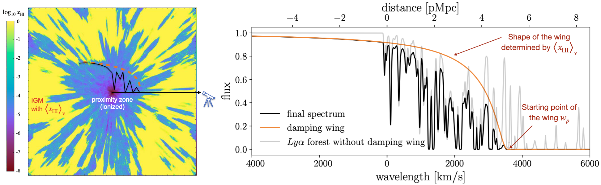
Figure 1: Left: A slice of a quasar proximity zone simulation [4]. Blue represents ionized gas while yellow indicates neutral gas. It also contains a cartoon illustrating the quasar spectrum: the blue region towards the observer corresponds to a ${\rm Ly}\alpha$ forest, enveloped by a damping wing (orange) arising from the neutral gas. Right: A spectrum simulated with the method described in Sec. 2. The final spectrum (black) is a multiplication of the ${\rm Ly}\alpha$ forest (grey) and the damping wing (orange).

2 Data

To accurately model the details in the proximity zone, we need hydrodynamical cosmological simulations and radiative transfer. However, simulating spectra with radiative transfer on-the-fly can be expensive. To reduce the simulating time, we develop a simulator that makes composite spectra using two pre-calculated datasets: proximity zone ${\rm Ly}\alpha$ forests and damping wings.

We create a set of proximity zone ${\rm Ly}\alpha$ forests by post-processing the Cosmic Reionization On Computers (CROC) simulations [13]. In each of the six $40~{}h^{-1}{\rm~{}cMpc}$ simulation boxes, we first select the 20 most massive halos. We then draw 50 sightlines with random orientations centered on each halo to sample the cosmological environments around quasars, and use 1D radiative transfer modelling [6] to create a large set of ${\rm Ly}\alpha$ spectra ranging from -4000 km/s to 8000 km/s.

To model damping wing components, we use the simulated damping wing database created by [5]. This database samples 10,000 sightlines traveling through different neutral patches in a universe with a given ${\left<x_{\rm HI}\right>_{\rm v}}$, capturing realistic scatter in the damping wing profile. The database is evenly spaced across 21 global neutral fractions ranging from ${\left<x_{\rm HI}\right>_{\rm v}}=0.995$ to ${\left<x_{\rm HI}\right>_{\rm v}}=0.008$. For each ${\left<x_{\rm HI}\right>_{\rm v}}$ and the starting point of the damping wing $w_{p}$, we then randomly draw one ${\rm Ly}\alpha$ forest and one damping wing with the closest ${\left<x_{\rm HI}\right>_{\rm v}}$. We then move the wing to $w_{p}$ and multiply the flux with the transmitted proportion of the wing on the red side and with zero on the blue side. We show an example of a simulated composite spectrum in the left panel of Fig. 2.

Real spectra usually have noise of varying levels. As a result, previous studies often have binned the data as a function of wavelength to reduce the effective noise per binned pixel [7]. In order to make realistic comparison between SBI and traditional pseudo-likelihood approach described in [7], we also bin our simulated quasar spectra to a similar resolution (500 km/s) over the entire spectral range in our subsequent tests (see the blue line in the left panel of Fig. 2 as an example). In the Supplementary Material, we show how the result changes with different noise levels and number of spectra used.

3 Methods

3.1 Simulation-Based Inference

We use the default Neural Posterior Estimation (NPE) [18, 14] framework as implemented by the sbipackage without any additional embedding network. The NPE aims to find the neural network (a density estimator) $\phi$ which maximizes $\Sigma_{i=0}^{i=N}\ln P(\theta_{i}|x_{i},\phi)$, where $(\theta_{i},x_{i})$ are independent (parameter, simulation) pairs generated from the prior. For the density estimator, we adopt Masked Autoregressive Flow (MAF) [19] trained on 100,000 simulated spectra. We run a small grid search for two hyper-parameters: the number of hidden features $n_{\rm hf}$ = ($5,10,20$) and number of transformations $n_{\rm t}=(5,10,20)$. We found that all the combinations return sensible results with clearly decoupled parameter constraints. We therefore opt to use MAF with the simplest hyper-parameter combination $(n_{\rm hf},n_{\rm t})=(5,5)$, which converged after 277 epochs.

3.2 Pseudo-likelihood Approach

In [7], a pseudo-likelihood $\tilde{L}(x|\theta)$ function is proposed to enable a Bayesian inference of ${\left<x_{\rm HI}\right>_{\rm v}}$ from quasar spectra. The pseudo-likelihood function is calculated by simply multiplying the likelihood for each wavelength bin assuming they are all independent:

$$\tilde{L}(x|\theta)=\prod_{i=1}^{n_{\rm bins}}\tilde{L}_{i}(x_{i}|\theta)$$ (1)

Similar to [7], we create a uniform grid of parameters with 21 bins in ${\left<x_{\rm HI}\right>_{\rm v}}$ and 16 bins in $w_{p}$ from 0 to 8000 km/s. We use the simulator described in Sec. 2 to generate 1000 spectra for each parameter pair (${\left<x_{\rm HI}\right>_{\rm v}}$, $w_{p}$). Then we use the distribution of flux values to estimate the flux probability distribution function (PDF) at each bin in order to evaluate the likelihood $\tilde{L}_{i}(x_{i}|\theta)$.

4 Results

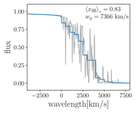
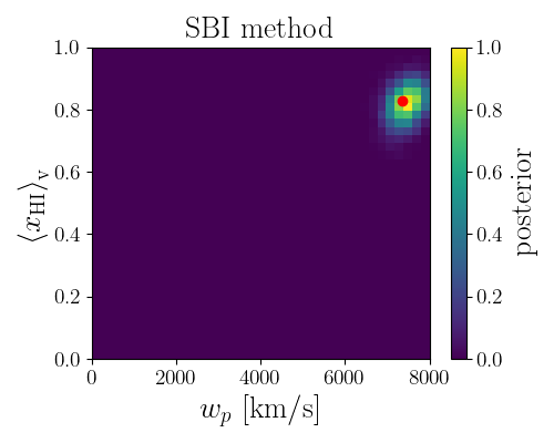
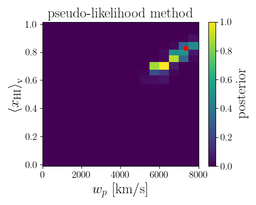
Figure 2: Left: An example of simulated spectra. The grey curve represents the high-resolution spectrum and the blue curve is the binned spectrum (bin size = 500 km/s) used as the summary statistics. Middle: Unnormalized posterior of the parameters infered by the SBI. Right: Unnormalized posterior using the traditional method with the “pseudo-likelihood" function. The right panel is at a lower resolution because the pseudo-likelihood is calculated on a uniform grid. The red point indicates the true parameters.

We use a uniform prior for both ${\left<x_{\rm HI}\right>_{\rm v}}$ and $w_{p}$. In the middle and right panels of Fig. 2, we show SBI and the pseudo-likelihood distributions for the example spectrum on the left panel. Compared with the SBI result in the middle panel, the pseudo-likelihood method shows stronger, more extended degeneracies between the two parameters and lower resolution due to the coarser input parameter grid, reliance on a single summary statistic $\tilde{L}$, and ignorance of potential intrapixel covariances. This degeneracy in the pseudo-likelihood method can be especially severe when $w_{p,\rm true}$ is large: for $w_{p}>w_{p,\rm true}$, many bins in Eq.1 have non-zero $\tilde{L}_{i}(x_{i}|\theta)$, which can be compensated with a stronger damping wing (smaller ${\left<x_{\rm HI}\right>_{\rm v}}$). On the other hand, SBI could extract the shape information of the damping wing from correlated pixels to break the degeneracy between the two parameters.

We also performed a probability calibration check [24] using the ranks of the estimated quantiles for 1000 test spectra to check whether there are biases across both sets of constraints (Fig. 3). We find that the rank distribution is consistent with a uniform distribution for both parameters ${\left<x_{\rm HI}\right>_{\rm v}}$ and $w_{p}$: comparing the rank distribution with the uniform distribution using the Kolmogorov–Smirnov (K-S) test, we obtain a $p$-value of 0.16 and 0.56 for ${\left<x_{\rm HI}\right>_{\rm v}}$ and $w_{p}$, respectively. This implies that there is no strong reason to believe that the collection of SBI PDFs do not accurately capture the scatter in true values given our estimated uncertainties.

From left to right, the blue histograms in Fig. 3 show the rank distribution, bias distribution and (two-sided) 68% interval of the ${\left<x_{\rm HI}\right>_{\rm v}}$ constraint from the SBI method, respectively. For a single spectrum, we find the root mean square (RMS) of bias in ${\left<x_{\rm HI}\right>_{\rm v}}$ to be $0.06$, which is smaller than the RMS of 68% scatter (0.12). Moreover, the typical scatter is approximately equal to the typical cosmic variance of the damping wing [5]. This demonstrates that SBI not only produces an unbiased inference of ${\left<x_{\rm HI}\right>_{\rm v}}$, but that these constraints are close to optimal.

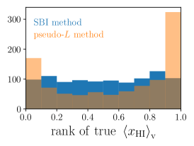
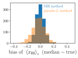
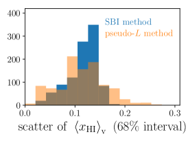
Figure 3: Rank distribution (left), bias (middle) and scatter (right) of the SBI method (blue) and the traditional method (orange). The number of test data points for both methods are 1000.

On the other hand, the traditional pseudo-likelihood method introduces significant bias. We show the rank distribution, bias and scatter of the inference on ${\left<x_{\rm HI}\right>_{\rm v}}$ in the faint orange histogram in Fig. 3. The “U” shape clearly demonstrates that the traditional method under-predicts the uncertainties in the inference. The RMS of the bias is $0.11$, larger than the SBI method. The RMS of the scatter of the pseudo-likelihood method (0.124) is similar to SBI (0.120), but the distribution is noticeably skewed towards both smaller and large values compared to SBI.

5 Discussion

We demonstrated that using SBI, we can more accurately constrain the neutral fraction of the universe using individual quasar spectra. SBI performs systematically better than traditional pseudo-likelihood methods, returning PDFs that are more accurate, and with more realistic uncertainties over our parameters of interest.

For an individual spectrum, the traditional method shows larger bias than the SBI method. Such bias could compromise our results when inferring from multiple spectra. Up to now, there are hundreds of quasars detected at $z>6$ with high-quality spectra, and one key step forward is to build an unbiased methodology to jointly constrain the global neutral fraction ${\left<x_{\rm HI}\right>_{\rm v}}$. From this perspective, the SBI method is clearly more desirable. The SBI can also be straight-forwardly implemented in such a multiple-spectra case by simply concatenating multiple spectra as input data.

6 Broader Impact

This is a pioneering study on using SBI with state-of-the-art radiative transfer cosmological simulations. The results show the promising potential of using quasar spectra to measure the detailed time evolution of the IGM ionization state, which is crucial for both cosmology and astrophysics. In the future, we will incorporate various realistic factors, especially continuum uncertainties [15, 8, 10, 17, 23] into the SBI framework and develop end-to-end machinery to uncover the reionization history. The methodology presented in this study can also be extended to detect and characterize different absorption systems such as Lyman Limit Systems or Damped ${\rm Ly}\alpha$ Absorbers in the ${\rm Ly}\alpha$ forest in quasar spectra [12, 22, 21], which is crucial for understanding structure formation.

7 Supplementary Material

7.1 Spectra with Noise

Real spectra always have some level of noise. Currently, the sample with the highest quality has an average signal-to-noise (SNR) $\sim 20$ per $10$ km/s [11]. We thus test how adding such noise impacts the results. In each spectrum, we first add an uncorrelated Gaussian noise with zero mean and a standard deviation of $5\%$ of the continuum level, and then bin it to $500$ km/s per bin. We again train a MAF with 5 hidden features and 5 transformations and test the results on a separate set of 1000 spectra with the same noise level. The simulation-based calibration shows the rank distributions are consistent with a uniform distribution for both ${\left<x_{\rm HI}\right>_{\rm v}}$ (K-S test $p$-value $=0.13$) and $w_{p}$ ($p$-value $=0.41$), indicating the uncertainties inferred from the SBI accurately capture the scatter in true values. The bias of each individual spectrum is increased slightly compared with the noiseless case: the RMS increases from $0.06$ to $0.09$ for ${\left<x_{\rm HI}\right>_{\rm v}}$, and from $505$ km/s to $775$ km/s for $w_{p}$, while the RMS scatter is increased from $0.12$ km/s to $0.18$ km/s for ${\left<x_{\rm HI}\right>_{\rm v}}$, and from $720$ km/s to $1120$ km/s for $w_{p}$ (see also Fig. 4).

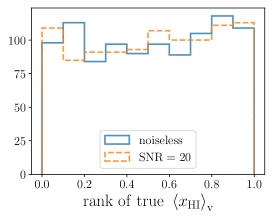
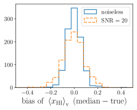
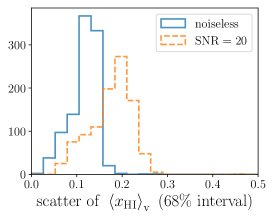
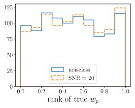
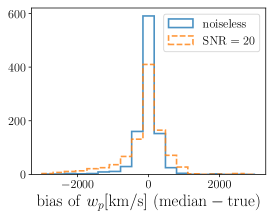
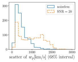
Figure 4: Comparison of rank distribution (left), bias (middle) and scatter (right) of the noiseless case (blue solid) and the SNR=20 case (orange dashed), both using SBI method. The number of test data points for both methods are 1000.

7.2 Scaling with Number of Spectra

Using multiple spectra at the same redshift could increase the constraint on ${\left<x_{\rm HI}\right>_{\rm v}}$. This is especially promising as we will have more reionization epoch quasars observed in the near future [3, 25]. Here we test how the inference scales with the number of spectra with different noise levels. Because we are primarily interested in ${\left<x_{\rm HI}\right>_{\rm v}}$, here we only train it to infer the single parameter ${\left<x_{\rm HI}\right>_{\rm v}}$. The input data for multiple spectra inference is constructed by simply concatenating the spectra together into a single 1D array.

We test a few realistic cases: SNR=5 for 1, 5 and 25 spectra and SNR=20 for 1 and 5 spectra. We use the same hyper-parameters ($n_{\rm hf}=5$, $n_{\rm t}=5$) and find that except for the single spectrum with SNR=5 case, all the others return an unbiased inference based on the K-S test on rank distribution with uniform distribution: the single SNR=5 spectrum case has $p$-value=0.008 while others all have $p$-value>0.05. For the single SNR=5 spectrum case, we further test other hyper-parameter combinations with $n_{\rm hf}$ varying between (3,5,10,20) and $n_{\rm t}$ varying between (2,3,5,10,20), but the highest $p$-value returned is still only $0.03$ (from combination $n_{\rm hf}=3$, $n_{\rm t}=2$). This indicates that using a single spectrum with only SNR=5, it is very challenging to obtain an accurate ${\left<x_{\rm HI}\right>_{\rm v}}$ constraint. In Fig. 5 we show the test results for each case, all trained with $n_{\rm hf}=5,n_{\rm t}=5$. For SNR=5 spectra, the RMS bias improves from 0.13, 0.069, to 0.044, and the RMS scatter improves from 0.25, 0.14 and 0.081 as we increase the number of spectra from 1, 5, to 25, respectively. On the other hand, for SNR=20 spectra, the RMS bias improves from 0.089 to 0.045 while the RMS scatter from 0.18 to 0.088 as we increase the number of spectra from 1 to 5.

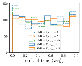
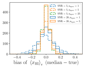
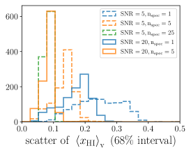
Figure 5: Rank distribution (left), bias (middle) and scatter (right) of cases of different number of spectra with different SNRs.

References

- [1] R Adam, N Aghanim, Mark Ashdown, J Aumont, C Baccigalupi, M Ballardini, AJ Banday, RB Barreiro, N Bartolo, Suman Basak, et al. Planck intermediate results-xlvii. planck constraints on reionization history. Astronomy & Astrophysics, 596:A108, 2016.
- [2] Nabila Aghanim, Yashar Akrami, Mark Ashdown, J Aumont, C Baccigalupi, M Ballardini, AJ Banday, RB Barreiro, N Bartolo, S Basak, et al. Planck 2018 results-vi. cosmological parameters. Astronomy & Astrophysics, 641:A6, 2020.
- [3] Rhys Barnett, SJ Warren, Daniel John Mortlock, J-G Cuby, C Conselice, PC Hewett, CJ Willott, NATALIA Auricchio, A Balaguera-Antolínez, Marco Baldi, et al. Euclid preparation-v. predicted yield of redshift 7< z< 9 quasars from the wide survey. Astronomy & Astrophysics, 631:A85, 2019.
- [4] Huanqing Chen. The role of quasar radiative feedback on galaxy formation during cosmic reionization. The Astrophysical Journal, 893(2):165, 2020.
- [5] Huanqing Chen. The characteristic shape of damping wings during reionization. Monthly Notices of the Royal Astronomical Society: Letters, page slad171, 2023.
- [6] Huanqing Chen and Nickolay Y Gnedin. The distribution and evolution of quasar proximity zone sizes. The Astrophysical Journal, 911(1):60, 2021.
- [7] Frederick B Davies, Joseph F Hennawi, Eduardo Bañados, Zarija Lukić, Roberto Decarli, Xiaohui Fan, Emanuele P Farina, Chiara Mazzucchelli, Hans-Walter Rix, Bram P Venemans, et al. Quantitative constraints on the reionization history from the igm damping wing signature in two quasars at z> 7. The Astrophysical Journal, 864(2):142, 2018.
- [8] Frederick B Davies, Joseph F Hennawi, Eduardo Banados, Robert A Simcoe, Roberto Decarli, Xiaohui Fan, Emanuele P Farina, Chiara Mazzucchelli, Hans-Walter Rix, Bram P Venemans, et al. Predicting quasar continua near ly with principal component analysis. The Astrophysical Journal, 864(2):143, 2018.
- [9] J Dunkley, R Hlozek, J Sievers, V Acquaviva, Peter AR Ade, P Aguirre, M Amiri, JW Appel, LF Barrientos, ES Battistelli, et al. The atacama cosmology telescope: cosmological parameters from the 2008 power spectrum. The Astrophysical Journal, 739(1):52, 2011.
- [10] Dominika Ďurovčíková, Harley Katz, Sarah EI Bosman, Frederick B Davies, Julien Devriendt, and Adrianne Slyz. Reionization history constraints from neural network based predictions of high-redshift quasar continua. Monthly Notices of the Royal Astronomical Society, 493(3):4256–4275, 2020.
- [11] Valentina D’Odorico, E Bañados, GD Becker, M Bischetti, SEI Bosman, G Cupani, R Davies, EP Farina, Andrea Ferrara, C Feruglio, et al. Xqr-30: The ultimate xshooter quasar sample at the reionization epoch. Monthly Notices of the Royal Astronomical Society, 523(1):1399–1420, 2023.
- [12] Roman Garnett, Shirley Ho, Simeon Bird, and Jeff Schneider. Detecting damped Ly absorbers with Gaussian processes. Mon. Not. Roy. Astron. Soc., 472(2):1850–1865, 2017.
- [13] Nickolay Y Gnedin. Cosmic reionization on computers. i. design and calibration of simulations. The Astrophysical Journal, 793(1):29, 2014.
- [14] David Greenberg, Marcel Nonnenmacher, and Jakob Macke. Automatic posterior transformation for likelihood-free inference. In International Conference on Machine Learning, pages 2404–2414. PMLR, 2019.
- [15] Bradley Greig, Andrei Mesinger, Zoltan Haiman, and Robert A Simcoe. Are we witnessing the epoch of reionization at z= 7.1 from the spectrum of j1120+ 0641? Monthly Notices of the Royal Astronomical Society, 466(4):4239–4249, 2017.
- [16] Laura C. Keating, Ewald Puchwein, James S. Bolton, Martin G. Haehnelt, and Girish Kulkarni. Investigating the characteristic shape and scatter of intergalactic damping wings during reionization, 2023.
- [17] Bin Liu and Rongmon Bordoloi. A deep learning approach to quasar continuum prediction. Monthly Notices of the Royal Astronomical Society, 502(3):3510–3532, 2021.
- [18] George Papamakarios and Iain Murray. Fast -free inference of simulation models with bayesian conditional density estimation. Advances in neural information processing systems, 29, 2016.
- [19] George Papamakarios, Theo Pavlakou, and Iain Murray. Masked autoregressive flow for density estimation. Advances in neural information processing systems, 30, 2017.
- [20] Michael Rauch. The lyman alpha forest in the spectra of qsos. Annual Review of Astronomy and Astrophysics, 36:267–316, 1998.
- [21] Keir K. Rogers, Simeon Bird, Hiranya V. Peiris, Andrew Pontzen, Andreu Font-Ribera, and Boris Leistedt. Correlations in the three-dimensional Lyman-alpha forest contaminated by high column density absorbers. Mon. Not. Roy. Astron. Soc., 476(3):3716–3728, 2018.
- [22] Keir K. Rogers, Simeon Bird, Hiranya V. Peiris, Andrew Pontzen, Andreu Font-Ribera, and Boris Leistedt. Simulating the effect of high column density absorbers on the one-dimensional Lyman forest flux power spectrum. Mon. Not. Roy. Astron. Soc., 474(3):3032–3042, 2018.
- [23] Zechang Sun, Yuan-Sen Ting, and Zheng Cai. Quasar factor analysis—an unsupervised and probabilistic quasar continuum prediction algorithm with latent factor analysis. The Astrophysical Journal Supplement Series, 269(1):4, 2023.
- [24] Sean Talts, Michael Betancourt, Daniel Simpson, Aki Vehtari, and Andrew Gelman. Validating bayesian inference algorithms with simulation-based calibration. arXiv preprint arXiv:1804.06788, 2018.
- [25] Wei Leong Tee, Xiaohui Fan, Feige Wang, Jinyi Yang, Sangeeta Malhotra, and James E Rhoads. Predicting the yields of > 6.5 quasar surveys in the era of roman and rubin. arXiv preprint arXiv:2308.12278, 2023.
- [26] Jinyi Yang, Feige Wang, Xiaohui Fan, Joseph F Hennawi, Frederick B Davies, Minghao Yue, Eduardo Banados, Xue-Bing Wu, Bram Venemans, Aaron J Barth, et al. Pōniuā ‘ena: A luminous z= 7.5 quasar hosting a 1.5 billion solar mass black hole. The Astrophysical Journal Letters, 897(1):L14, 2020.
- [27] O Zahn, CL Reichardt, L Shaw, A Lidz, KA Aird, BA Benson, LE Bleem, JE Carlstrom, CL Chang, HM Cho, et al. Cosmic microwave background constraints on the duration and timing of reionization from the south pole telescope. The Astrophysical Journal, 756(1):65, 2012.