1 Introduction

Models of inflation have been obtained under the assumption that the kinetic term of an inflaton scalar $\phi$ contains a non-integrable pole at some field value $\phi=\phi_{\rm pole}$

$$\mathscr{L}=K(\phi)\frac{(\partial_{\mu}\phi)^{2}}{2}-V(\phi),\qquad K(\phi)\sim\left|\frac{\phi_{*}}{\phi-\phi_{\rm pole}}\right|^{p},\qquad p\geq 2.$$ (1)

Indeed, after canonicalisation of $\phi$ into $\phi_{\rm can}$, the Lagrangian simplifies to

$$\mathscr{L}=\frac{(\partial_{\mu}\phi_{\rm can})^{2}}{2}-V_{\rm can}(\phi_{\rm can})$$ (2)

where the scalar potential $V_{\rm can}$ undergoes an infinite stretch, acquiring the flatness needed to support inflation. Pole inflation models have been motivated invoking string theory, supergravity [1, 2, 3, 4] or a non-minimal scalar coupling $f(\phi)R$ to gravity [5].

We here consider a milder integrable pole with $0<p<2$, equivalent to a finite stretch of the inflaton potential, and thereby to an exact inflection point in the canonical potential. This can give interesting signals if $\phi$ is the inflaton. Indeed it is known that an approximate inflection point in an inflationary potential, characterized by a small $V^{\prime}$, leads to a phase with an amplified power spectrum of primordial inhomogeneities $P_{\zeta}\propto 1/V^{\prime 2}$ which subsequently gives rise to scalar-induced gravitational waves and to primordial black holes [6, 7, 8, 9, 10, 11, 12, 13, 14, 15, 16, 17, 18, 19, 20, 21, 22, 23, 24, 25]. We will discuss that an exact inflection point, as obtained from a traversable integrable pole, also gives these signals.

In section 2 we present the correspondence between the kinetic function $K(\phi)$, the potential $V(\phi)$ and the canonical potential $V_{\rm can}(\phi_{\rm can})$. In section 3 we set up the formalism to conveniently compute keeping $K\neq 1$, avoiding the canonicalisation that trades a pole $K(\phi_{\rm pole})=\infty$ for an inflection point in $V_{\rm can}$. In section 4 we compute the predicted power spectrum $P_{\zeta}(k)$. In section 5 we compute the resulting frequency spectrum $\Omega_{\rm GW}(f)$ of gravitational waves generated at second order in $P_{\zeta}$. In section 6 we determine the resulting mass spectrum of primordial black holes. Section 4.2 will show that $p<1$ allows to obtain such signals without a large tuning of model parameters.

In section 7 we introduce a potential theoretical explanation for the existence of an integrable pole. Some particles with Planck-scale mass (such as string states) might become massless at a point $\phi=\phi_{\rm pole}$ in field space, during the inflaton’s Planckian journey in field space. Light particles induce quantum corrections to the kinetic function of $\phi$ that can lead to a pole-like structure, with a value of $p$ related to the anomalous dimension of $\phi$. Some particle interactions contribute as $p<0$, leading to a vanishing $K$ rather than to a pole: after canonicalisation this is equivalent to a jump-like feature in the inflaton potential: we also mention the consequent signals [28, 29].

Conclusions are given in section 8.

2 Potential for the canonical inflaton

We work in the Einstein frame, where scalars have minimal coupling to gravity (so that the graviton kinetic term is canonical), and can have a non-canonical kinetic function $K(\phi)$ in the action:

$$S=\int d^{4}x\sqrt{|\det g|}\bigg{[}-\frac{\bar{M}_{\rm Pl}^{2}}{2}R+\frac{K(\phi)}{2}{(D_{\mu}\phi)(D^{\mu}\phi)}-V(\phi)+\cdots\bigg{]}.$$ (3)

We assume one scalar $\phi$ with one pole at $\phi=\phi_{\rm pole}$. With one scalar only, the non-canonical kinetic term $K$ can be reabsorbed by defining a canonically normalised scalar $\phi_{\rm can}(\phi)$ as $d\phi_{\rm can}/{d\phi}=\sqrt{K}$. In this section we discuss how the pole is equivalent to a feature in the canonical potential

$$V_{\rm can}(\phi_{\rm can})=V(\phi(\phi_{\rm can})).$$ (4)

We assume a kinetic function with a pole ($p>0$) or a dip ($p<0$):

$$K(\phi)=\left\{\begin{array}[]{ll}\displaystyle 1+\left|\frac{\phi_{*}}{\phi-\phi_{\rm pole}}\right|^{p}&\hbox{for }p>0\\ \displaystyle\left[1+\left|\frac{\phi_{*}}{\phi-\phi_{\rm pole}}\right|^{-p}\right]^{-1}&\hbox{for }p<0\end{array}\right.\stackrel{{\scriptstyle\phi\to\phi_{\rm pole}}}{{\simeq}}\left|\frac{\phi_{*}}{\phi-\phi_{\rm pole}}\right|^{p}.$$ (5)

The term $1$ makes the kinetic term canonical, away from the special point $\phi_{\rm pole}$. The full $\phi_{\rm can}(\phi)$ resulting from the $K(\phi)$ in eq. (5) can be written in terms of hypergeometric functions. We will later more simply compute inflation without performing the canonicalisation, and we here discuss the effect of canonicalisation around the special point $\phi_{\rm pole}$, where one can neglect this constant term in $K$, obtaining for any $p$

$$\frac{\phi_{\rm can}-\phi_{\rm pole}}{\phi_{*}}\simeq d\left|\frac{\phi-\phi_{\rm pole}}{\phi_{*}}\right|^{1/d},\qquad d\equiv\frac{2}{2-p}=\left\{\begin{array}[]{ll}1&\hbox{for }p=0\\ 2&\hbox{for }p=1\\ 3&\hbox{for }p=4/3\end{array}\right.~{}.$$ (6)

Eq. (6) means that the parameter $d$ is the dimension of the field $\phi$ around the pole. In section 7 we will interpret $d\neq 1$ as a quantum anomalous dimension.

2.1 Kinetic function with a pole, $p>0$

Let us first consider the pole case, corresponding to $p>0$. In line with the literature on pole inflation, we make the assumption that the pole in the kinetic term is not accompanied by a non-trivial feature in the potential. As a result, the potential can be approximated through a first-order Taylor expansion. Therefore, we proceed with the assumption that, around the pole,

$$V(\phi)\simeq V_{0}+V^{\prime}_{0}(\phi-\phi_{\rm pole}).$$ (7)

Significant changes occur at two critical values: $p=1$ and $p=2$.

A pole with $p\geq 2$ is non-integrable: the $\phi$ region near the pole becomes an infinite range of the canonical $\phi_{\rm can}$ field, so the potential gets infinitely stretched acquiring a nearly-flat inflationary form [1, 2, 3, 4, 5].

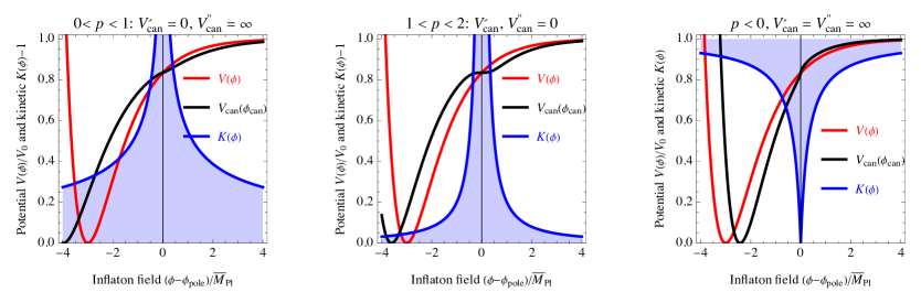
Figure 1: How a kinetic function $K(\phi)$ as in eq. (5) (in blue) modifies an inflaton potential $V(\phi)$ as in eq. (21) (in red), rewriting the system as a potential $V_{\rm can}(\phi_{\rm can})$ (in black) for the canonical field $\phi_{\rm can}$. Left: traversable pole with low $p<1$, such that $V_{\rm can}^{\prime}=0$ and $V_{\rm can}^{\prime\prime}=\infty$ at the pole. Middle: traversable pole with $p=4/3$ such that $V_{\rm can}$ is cubic around the inflection point. Right: dip with $p<0$ such that $V_{\rm can}$ develops a jump. The position $\phi_{\rm pole}$ of the pole and its thickness $\phi_{*}$ are free parameters.

This paper focuses instead on an integrable pole with $0<p<2$, that gives a finite stretching of the potential around the pole, where the potential acquires the form of an exact inflection point

$$V_{\rm can}(\phi_{\rm can})\simeq V_{\rm pole}(\phi_{\rm can})\equiv V_{0}\left[1+\left(\frac{\phi_{\rm can}-\phi_{\rm pole}}{\phi_{0}}\right)^{d}\right]\qquad\hbox{where}\qquad\phi_{0}=\phi_{*}d\left(\frac{V_{0}}{V^{\prime}_{0}\phi_{*}}\right)^{1/d}.$$ (8)

We introduced the parameter $\phi_{0}$ and left understood how to deal with non-integer $d$ at $\phi_{\rm can}<\phi_{\rm can}^{\rm pole}$. The first derivative vanishes at the pole, $V^{\prime}_{\rm can}(\phi_{\rm pole})=0$, so the associated slow-roll parameter $\epsilon_{V}\propto V^{\prime 2}_{\rm can}$ vanishes. In the slow-roll approximation the power spectrum $P_{\zeta}=H^{2}/8\pi^{2}\bar{M}_{\rm Pl}^{2}\epsilon_{V}$ diverges, hinting that the slow-roll approximation breaks down and $P_{\zeta}$ is enhanced. Two sub-cases need to be considered:

• If $1<d<2$ (corresponding to $0<p<1$) the number of $e$-folds computed in slow-roll approximation (eq. (12) later) remains finite, and the second derivative $\eta_{V}\propto V^{\prime\prime}_{\rm can}$ diverges at $\phi_{\rm pole}$ breaking the slow-roll approximation. The modified kinetic term stretches the field space also away from $\phi_{\rm pole}$. The left panel of fig. 1 shows an example.

• If $d>2$ (corresponding to $p>1$) the pole has a local effect, producing an exact inflection point where $V^{\prime}_{\rm can}=V^{\prime\prime}_{\rm can}=0$ and thereby both slow-roll parameters vanish. The middle panel of fig. 1 shows an example with $d=3$. The pole is only traversed beyond the slow-roll approximation, that breaks down. The $V_{\rm can}\simeq V_{\rm pole}$ approximation only holds in a field region with size $\Delta\phi\sim\phi_{*}$ around the pole. Outside this region $K\simeq 1$ so that $V_{\rm can}(\phi_{\rm can})\simeq V(\phi+\Delta)$ where $\Delta$ is some finite shift due to the stretching occurred around the pole.

Assuming that $V(\phi)$ globally has inflationary form, we can now discuss the inflationary consequences of a traversable pole. If the $V_{\rm pole}$ approximation of eq. (8) were applicable away from the pole, the slow-roll parameters would get large at $|\phi_{\rm can}-\phi_{\rm pole}|\gtrsim\phi_{0}$. However it’s important to note that eq. (8) only holds in a narrow field range with size $\Delta\phi$ around the pole. We will be interested in $\Delta\phi\ll\phi_{0}$, such that the slow-roll parameters can be always small.

2.2 Kinetic function with a dip, $p<0$

The kinetic function $K$ vanishes at the special point $\phi_{\rm pole}$ if $p<0$. Infinitesimally near to $\phi_{\rm pole}$ the canonical potential is approximated by eq. (8) where now $0<d<1$. This means that the canonical potential develops a jump, where $V^{\prime}_{\rm can}=V^{\prime\prime}_{\rm can}=\infty$. An example of such a scenario is displayed in the right panel of fig. 1.

We anticipate that a jump tends to produce a mild oscillatory feature in the power spectrum $P_{\zeta}(k)$. However, in certain cases, a more significant amplification of $P_{\zeta}$ can occurr: a) from a series of sharp jumps [28, 29], which would correspond to a series of poles with $p\ll-1$. b) from a very small value of the slow-roll parameter $\epsilon$ away from the pole, as possible in small-field inflation [29]. This would give distinctive features in $P_{\zeta}(k)$, that get imprinted in the gravitational wave spectrum. For the remainder of this paper, we will focus on cases where $p>0$ and avoid pursuing these dip possibilities.

3 The formalism for computing inflation

In this section we recall the standard formulæ that will be later used to compute inflation in the theory of eq. (3), with a generic inflaton potential $V$ and a generic kinetic function $K$. The $\Lambda$CDM best-fit values of the scalar tilt $n_{s}$, of the power spectrum of scalar perturbations $P_{\zeta}(k)$, and of the tensor-to-scalar ratio $r=P_{h}/P_{\zeta}$ from Planck-BICEP at the CMB pivot scale $k\approx 0.056/{\rm Mpc}$ are [30]

$$n_{s}=0.9649\pm 0.0042,\qquad P_{\zeta}\approx(2.1\pm 0.06)\times 10^{-9},\qquad r\lessapprox 0.035$$ (9)

around cosmological scales corresponding to $N\approx 50-60$ $e$-folds before the end of inflation. Larger ranges are found in $\Lambda$CDM extensions. The classical inflaton equation of motion is

$$\ddot{\phi}+\frac{K^{\prime}}{K}\frac{\dot{\phi}^{2}}{2}+3H\dot{\phi}+\frac{V^{\prime}}{K}=0.$$ (10)

3.1 The slow-roll approximation

The slow-roll approximation neglects the first two terms in eq. (10). In the slow-roll limit, the slow-roll parameters are given by [31, 32]

$$\epsilon_{V}\equiv-\frac{\dot{H}}{H^{2}}\simeq\frac{1}{2}\frac{\bar{M}_{\rm Pl}^{2}}{K}\frac{V^{\prime 2}}{V^{2}},\qquad\eta_{V}\equiv\frac{\dot{\epsilon}_{V}}{H\epsilon_{V}}\simeq\frac{\bar{M}_{\rm Pl}^{2}}{K}\frac{V^{\prime}}{V}\frac{d\ln\epsilon_{V}}{d\phi}.$$ (11)

Inflation ends when $\epsilon_{V}(\phi_{\rm end})\approx 1$ and the number of $e$-foldings is given by

$$N(\phi)=\int_{\phi_{\rm end}}^{\phi}d\phi^{\prime}\ \frac{K(\phi^{\prime})}{\bar{M}_{\rm Pl}^{2}}\frac{V(\phi^{\prime})}{V^{\prime}(\phi^{\prime})}.$$ (12)

The predictions for $n_{s}$, $P_{\zeta}$ and $r$ are well known,

$$n_{s}=1-2\epsilon_{V}+\eta_{V},\qquad P_{\zeta}=\frac{1}{24\pi^{2}}\frac{V}{\bar{M}_{\rm Pl}^{4}\epsilon_{V}},\qquad r=16\epsilon_{V}$$ (13)

evaluated around horizon crossing. The power spectrum of eq. (13) diverges at $\phi_{\rm pole}$ as the kinetic function diverges, $K\to\infty$, leading to $\epsilon_{V}\to 0$. Furthermore, this point is non-traversable in slow-roll approximation if $p>1$, as eq. (12) diverges. In any case the slow-roll approximation breaks down around the pole when $\eta_{V}\sim 1$ corresponding to $(V^{\prime}/\sqrt{K})^{\prime}/\sqrt{K}\sim H^{2}$.

3.2 Classical motion beyond the slow-roll limit

We thereby solve the full classical equation of motion, using the number of $e$-folds $dN=H\,dt$ rather than time $t$ as variable:

$$\frac{1}{3-\epsilon_{H}}\left(K\frac{d^{2}\phi}{dN^{2}}+\epsilon_{H}\frac{\bar{M}_{\rm Pl}^{2}K^{\prime}}{K}\right)+K\frac{d\phi}{dN}+\bar{M}_{\rm Pl}^{2}\frac{V^{\prime}}{V}=0$$ (14)

where

$$H^{2}=\frac{V}{\bar{M}_{\rm Pl}^{2}(3-\epsilon_{H})},\qquad\epsilon_{H}=\frac{d\ln H}{dN}=\frac{K}{2\bar{M}_{\rm Pl}^{2}}\left(\frac{d\phi}{dN}\right)^{2}\qquad\hbox{and}\qquad\eta_{H}=\epsilon_{H}-\frac{1}{2\epsilon_{H}}\frac{d\epsilon_{H}}{dN}$$ (15)

will be used later. Eq. (14) will be numerically solved starting from the slow-roll initial condition $d\phi/dN=-\bar{M}_{\rm Pl}^{2}V^{\prime}/KV$. This provides the approximation for $n_{s}$, $P_{\zeta}$ and $r$ known as ‘exact slow-roll’. Following the notations of [19]:

$$n_{s}=1-4\epsilon_{H}+2\eta_{H},\qquad P_{\zeta}=\frac{1}{24\pi^{2}}\frac{V}{\bar{M}_{\rm Pl}^{4}\epsilon_{H}},\qquad r=16\epsilon_{H}.$$ (16)

This power spectrum qualitatively differs from the slow-roll approximation in eq. (13) at the pole point where $\epsilon_{V}=0$ while $\epsilon_{H}\neq 0$.

3.3 Mukhanov-Sasaki equations

To precisely compute the power spectrum $P_{\zeta}(k)$ one needs to expand the field $\phi$ into fluctuating modes $\phi_{k}$ with co-moving momentum $k$ and solve the equations for their inflationary evolution. As usual it is convenient to consider the gauge-invariant combination $\zeta=-\psi+H\delta\phi/\dot{\phi}$ of the inflaton $\phi$ and the gravity potential $\psi$. The power spectrum is obtained as $P_{\zeta}=k^{3}|\zeta_{k}|^{2}/2\pi^{2}$ from the values of the complex modes $\zeta_{k}$ at inflation end. Defining $v_{k}=-z\zeta_{k}$ where $z^{2}=2a^{2}\epsilon_{H}$ and $a=e^{N}$ is the scale factor, the Mukhanov-Sasaki (MS) equation for $v_{k}$ is

$$\frac{d^{2}v_{k}}{dN^{2}}+(1-\epsilon_{H})\frac{dv_{k}}{dN}+\left[\frac{k^{2}}{a^{2}H^{2}}+(1+\epsilon_{H}-\eta_{H})(\eta_{H}-2)-\frac{d(\epsilon_{H}-\eta_{H})}{dN}\right]v_{k}=0.$$ (18)

Eq. (18) can be numerically solved starting from the Bunch-Davies initial condition

$$v_{k}=\frac{1}{\sqrt{2k}},\qquad\frac{dv_{k}}{dN}=\frac{kv_{k}}{iaH}.$$ (19)

In numerical computations it is more convenient to solve the equation for $\zeta_{k}$

$$\frac{d^{2}\zeta_{k}}{dN^{2}}+f\frac{d\zeta_{k}}{dN}+\frac{k^{2}}{a^{2}H^{2}}\zeta_{k}=0,\qquad f=3+\epsilon_{H}-2\eta_{H}$$ (20)

because no $\phi^{\prime\prime\prime}$ is involved. A negative $f<0$ signals amplification of $\zeta_{k}$. The number of $e$-folds $N=\ln k/k_{\rm end}$ is converted into the wave-number $k$ by computing $k_{\rm end}$, the scale corresponding to inflation end, assuming instantaneous reheating with temperature $T_{\rm RH}=(30V(\phi_{\rm end})/\pi^{2}g)^{1/4}$ where $g=106.75$ is the number of Standard Model degrees of freedom. Standard big-bang cosmology then gives the scale factor at inflation end, $a_{\rm end}=a_{\rm eq}(g_{s\rm eq}T_{\rm eq}/gT_{\rm RH})^{1/3}$ in terms of $g_{s\rm eq}=43/11$, $T_{\rm eq}\approx 0.74\,{\rm eV}$, $a_{\rm eq}\approx 1/3100$.

3.4 The inflationary potential

As a concrete example, we assume the inflationary potential

$$V=V_{0}\left[1-e^{-\sqrt{2/3}\phi/\bar{M}_{\rm Pl}}\right]^{2}$$ (21)

independently motivated by $R^{2}$ gravity [34], by $\alpha$-attractor models [1, 2, 3, 4], and by Higgs-like scalar inflation with large non-minimal scalar coupling to gravity $\xi\gg 1$ [35]. Without a kinetic pole, the inflaton potential assumed in eq. (21) leads to $n_{s}=1-2/N$ and $r=12/N^{2}$, in agreement with $\Lambda$CDM best fits for $N\sim(50-60)$.

4 The power spectrum

We now use the formalism of section 3 to compute inflation in the theory of eq. (3). Following the classification of section 2 a pole with $1<p<2$ is considered in section 4.1, while $0<1<p$ is considered in section 4.2.

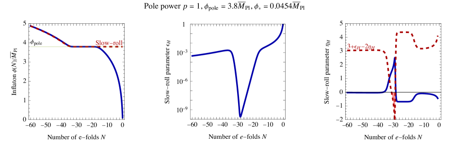
Figure 2: Sample of inflationary evolution as function of the number of $e$-folds $N$ for pole power $p=1$. Left: the inflaton field $\phi$ compared to the slow-roll approximation. Middle: the $\epsilon_{H}$ parameter. Right: the $\eta_{H}$ parameter and $f=3+\epsilon_{H}-2\eta_{H}$. Amplification of $P_{\zeta}$ occurs for $f<0$, in the shaded region.

4.1 Pole exponent $1\leq p<2$

The number of $e$-folds in slow-roll approximation $N\propto\int d\phi~{}K$ diverges around a pole with $p\geq 1$, corresponding to an inflection point, as exemplified by the dashed curve in the left panel of fig. 2. So a pole with $1\leq p<2$ is not traversed in slow-roll approximation, and we need to solve the full eq. (14).

We first present a simple analytic argument showing that the pole is traversed as long as the pole width is sub-Planckian, $\phi_{*}\lesssim 0.1\bar{M}_{\rm Pl}$. Making the field canonical the pole is transformed into an inflection point that can be roughly approximated as a field range

$$\Delta\phi_{\rm can}=\int_{-\phi_{\rm max}}^{+\phi_{\rm max}}d\phi\,(\sqrt{K}-1)\sim\phi_{*}\left[\frac{4}{2-p}+\frac{1-(\phi_{*}/\phi_{\rm max})^{p-1}}{p-1}\right]\qquad\hbox{for $0<p<2$}$$ (22)

within which the potential is constant, $V^{\prime}_{\rm can}=0$ and $K_{\rm can}=1$. The slow-roll approximation breaks down when the inflaton enters the flat region with initial speed $\dot{\phi}_{\cancel{\rm SR}}\simeq\sqrt{2\epsilon_{\cancel{\rm SR}}}H\bar{M}_{\rm Pl}$ where $\epsilon_{\cancel{\rm SR}}\ll 1$ is the $\epsilon_{V}$ slow-roll parameter of the inflationary potential $V$ just away from the pole. Inside the nearly-flat pole region, the inflaton proceeds inertially according to $\ddot{\phi}_{\rm can}+3H\dot{\phi}_{\rm can}=0$, evolving by an amount $\phi_{\rm walk}=\dot{\phi}_{\cancel{\rm SR}}/3H$ before being stopped by Hubble friction. Thereby the flat interval is traversed if

$$\Delta\phi_{\rm can}\lesssim\phi_{\rm walk}\approx\sqrt{2\epsilon_{\cancel{\rm SR}}}\bar{M}_{\rm Pl}/3.$$ (23)

This means that a sub-Planckian pole $\phi_{*}\ll\bar{M}_{\rm Pl}$ is traversed. After entering the flat region at $N=N_{\cancel{\rm SR}}$ $e$-folds, the inflaton slows down increasing the power spectrum as $P_{\zeta}\sim P_{\zeta\cancel{\rm SR}}\,\exp(6(N-N_{\cancel{\rm SR}}))$. A large enhancement of $P_{\zeta}$ arises if the inflaton significantly slows down, corresponding to eq. (23) being nearly saturated. Above this value the classical approximation breaks down as $P_{\zeta}\sim 1$. We are interested in $P_{\zeta}$ enhanced up to $10^{-2}$ as needed to form an allowed amount of primordial black holes and/or generating a detectable allowed amount of gravitational waves. We thereby select the value of $\phi_{*}$ in eq. (5) such that $P_{\zeta}(k)\lesssim 10^{-2}$. Table 1 shows that such a large enhancement in $P_{\zeta}(k)$ needs a tuning of $\phi_{*}$ of order $(P_{\zeta}/10^{-9})^{1/2}\sim 10^{3}$ [36].

The shaded regions are excluded by the current constraint on CMB $\mu$-distortion, $|\mu|<0.9~{}10^{-4}$ [37] and by the effect on the neutron/proton abundance during big-bang nucleosynthesis [38]. The dashed curve represents the future PIXIE sensitivity on $\mu$-distortion [39], down to $|\mu|\sim 10^{-7}$.

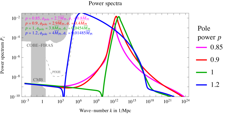
Figure 3: Sample of power spectra for different pole powers $p$. For $p\geq 1$ the value of $\phi_{*}$ is tuned such that $P_{\zeta}$ reaches $\sim 10^{-2}$. The gray regions are excluded by CMB, LSS, COBE-$\mu$, COBE-$y$, AR [40]; the dashed curve is the sensitivity of PIXIE [39].

$$\begin{array}[]{c|ccc}\lx@intercol\hfil\hbox{Fine tuning $\Delta_{x}=\partial\ln P_{\zeta}^{\rm peak}/\partial\ln x$}\hfil\lx@intercol\cr\hline\cr\hbox{Sample}&\lx@intercol\hfil\hbox{Theory parameters}\hfil\lx@intercol\cr\hbox{spectrum}&x=\phi_{*}&x=\phi_{\rm pole}&x=p\cr\hline\cr\color[rgb]{1,0,0}p=0.9&\Delta=4&\Delta=15&\Delta=35\cr\color[rgb]{0,0.6,0.01}p=1&\Delta=25&\Delta=80&\Delta=165\cr\color[rgb]{0,0,1}p=1.2&\Delta=130&\Delta=400&\Delta=400\cr\end{array}$$

Table 1: Fine-tuning sensitivities $\Delta_{x}$ of $P_{\zeta}^{\rm peak}=\max_{k}P_{\zeta}(k)$ to theory parameters $x$ for the sample spectra that achieve $P_{\zeta}^{\rm peak}\approx 0.01$ with different values of the pole power $p$.

Fig. 3 shows examples of the power spectra for a pole with the critical power $p=1$ (corresponding to $d=2$, a quadratic canonical potential around the pole) and for other values of $p$ around 1. Fig. 2 shows additional details of the inflationary evolution in the $p=1$ example. The power spectrum, obtained solving the MS equation, is well approximation by eq. (16) which, in turn, differs from the approximation of eq. (13) only for the narrow spike at the pole. This $p=1$ example gives $n_{s}\approx 0.952$ and $r\approx 0.003$ at the CMB pivot scale, as can be understood by noticing that the inflaton pausing around the pole reduces its field value corresponding to the CMB scale. These values are compatible with simple $\Lambda$CDM extensions (e.g. [41]), and the best-fit $\Lambda$CMD value of $n_{s}$ could be obtained by assuming a different potential above the integrable kinetic pole. A suitable choice is a generic potential made inflationary by an extra non-integrable pole with $p^{\prime}>2$, see eq. (10) of [5]. Table 1 shows that the $p=1$ critical case is less strongly tuned than $p>1$.

The behaviour of $P_{\zeta}(k)$ is understood as follows:

1. While $\phi$ approaches $\phi_{\rm pole}$, $P_{\zeta}(k)$ quickly grows roughly proportionally to $e^{6N}\propto k^{6}$.

2. Around the pole $P_{\zeta}(k)$ reaches a maximal value well approximated by eq. (16), $\max P_{\zeta}\approx V_{0}/24\pi^{2}\bar{M}_{\rm Pl}^{2}\epsilon_{H}^{\rm min}$. The minimal value of $\epsilon_{H}$ depends on the $\phi_{*}$ parameter. Furthermore, the scale $k$ at which $P_{\zeta}$ is maximal depends on the value of $\phi_{\rm pole}$.

3. After crossing the pole, $P_{\zeta}$ slowly decreases as the inflaton reaccelerates. A new slow-roll approximation shows that this phase lasts $\Delta N\sim(\phi_{0}/\bar{M}_{\rm Pl})^{2/p}(\epsilon_{H}^{\rm min})^{(1-p)/p}$ $e$-folds. An enhancement of $P_{\zeta}$ up to $10^{-2}$ needs a small $\epsilon_{H}^{\rm min}$. So a too long $\Delta N\gtrsim 50$ is avoided if $p$ is mildly close to 1: $p\lesssim 4/3$ corresponding to a cubic $d=3$ inflection point in $V_{\rm can}$. The numerical result in fig. 3 confirms that, for $p=1.2$ and for the inflationary potential of eq. (21), $P_{\zeta}$ can peak at small enough $k\lesssim 1/{\rm kpc}$, while satisfying COBE-FIRAS bounds [40] and giving signals in PIXIE [39].

For the values of $1<p<2$ considered here the kinetic function $K$ deviates from 1 only in a narrow region around the pole, so that inflationary predictions away from the pole are not affected by the pole.

4.2 Pole exponent $0<1<p$

If $p<1$ the kinetic function $K$ deviates from 1 also away from the pole, as clear from the fact that the field range of eq. (22) receives a contribution from $\phi_{\rm max}$. As a result $P_{\zeta}$ and $n_{s}$ at CMB scales are affected by the pole, and the traversability approximation of eq. (23) no longer applies. Rather, the pole is always traversed, even in slow-roll approximation. Increasing the parameter $\phi_{*}$ no longer allows to arbitrarily increase $P_{\zeta}$ at the price of a tuning.

Numerical solutions show that a significant enhancement of $P_{\zeta}$ still arises for $p$ mildly below 1, $0.85\lesssim p<1$. Fig. 3 shows examples for $p=0.9$ and for $p=0.85$. The value $p=0.85$ only leads to a mild enhancement in $P_{\zeta}$, while a large enhancement up to $0.01$ still arises for $p=0.9$. Table 1 shows an interesting feature of the $p=0.9$ example: the logarithmic sensitivities with respect to all parameters of the theory are mild, indicating the large enhancement of $P_{\zeta}$ is achieved without a strong tuning. This is interesting, given that several single-field inflation models lead to a strong enhancement of the primordial power spectrum at small scales at the price of a strong fine-tuning [36], related to the fact that the enhancement typically requires an ultra-flat region of the scalar field potential over a small field range. The tuning issue also affects other models, like those with transient inflationary features in the primordial power spectrum or new phase transitions (see [43] for a review).

We also see that $p<1$ gives peaks in $P_{\zeta}(k)$ with a different shape than $p>1$: a slower growth before the peak, a shaper peak, a faster decrease after the peak. The critical case $p=1$ results in a shape that is intermediate between the characteristic shapes associated with $p>1$ and $p<1$. This shape will have an impact on the spectrum of gravitational waves, which will be the subject of discussion in the next section.

5 Scalar-induced gravitational waves

The primordial spectrum of scalar inhomogeneities $P_{\zeta}(k)$ induces a spectrum of gravitational waves with density $\Omega_{\rm GW}(f)\sim 10^{-5}P_{\zeta}^{2}(2\pi f)$ [44, 45, 46, 47, 48, 49]. We start by summarising in section 5.1 how $\Omega_{\rm GW}$ is precisely computed, and present results in section 5.2.

5.1 The formalism for computing gravitational waves

First-order inflaton cosmological perturbations, described by the power spectrum $P_{\zeta}$ of curvature scalar perturbations, induce gravitational waves, often referred to as Scalar Induced Gravitational Waves (SIGW), at second order in cosmological perturbation theory [50, 45]. These gravitational waves are described by transverse-traceless tensor perturbations $h_{ij}$ in the metric. This gravitational effect is conveniently computed using the Newtonian gauge where the inflaton is homogeneous and the first-order scalar perturbations are described by one potential $\psi$, while neglecting anisotropic stress. The metric is

$$\mathrm{d}s^{2}=-(1+2\psi)\mathrm{d}t^{2}+a(t)^{2}\left[(1-2\psi)\delta_{ij}+h_{ij}\right]\mathrm{d}x^{i}\mathrm{d}x^{j}~{},$$ (24)

The $h_{ij}$ of eq. (24) are inevitably induced via non-linear coupling between different modes of the first-order scalar modes of $\psi$. At second perturbative order, the tensor modes with helicity $\lambda$ evolve in conformal time $\tau$ as

$$h_{\bm{k}}^{\lambda\prime\prime}(\tau)+2aHh_{\bm{k}}^{\lambda\prime}(\tau)+k^{2}h_{\bm{k}}^{\lambda}(\tau)=S^{\lambda}_{\bm{k}}(\tau)~{},$$ (25)

where the source term $S^{\lambda}_{\bm{k}}$ during radiation domination is

$$S^{\lambda}_{\bm{k}}=2\int{\mathrm{d}^{3}\bm{p}\over(2\pi)^{3/2}}\bm{e}^{\lambda}(\bm{k},\bm{p})\Big{[}3\psi_{\bm{p}}\psi_{\bm{k}-\bm{p}}+\frac{\psi_{\bm{p}}^{\prime}\psi^{\prime}_{\bm{k}-\bm{p}}}{a^{2}{H}^{2}}+\frac{\psi_{\bm{p}}^{\prime}\psi_{\bm{k}-\bm{p}}+\psi_{\bm{p}}\psi^{\prime}_{\bm{k}-\bm{p}}}{a{H}}\Big{]}~{},$$ (26)

$\bm{e}^{\lambda}(\bm{k},\bm{p})\equiv e^{\lambda}_{lm}(\bm{k})p_{l}p_{m}$ and all $\psi$ are evaluated at $\tau$. Substituting $\psi_{k}=2\zeta_{k}/3$ [51], solving eq. (25) via the Green function method and summing over polarizations gives the SIGW power spectrum [46, 52]

$$\mathcal{P}_{h}(\tau,k)=\int^{\infty}_{0}\mathrm{d}v\int^{|1+v|}_{|1-v|}\mathrm{d}u\left[{4v^{2}-(1+v^{2}-u^{2})^{2}\over 4uv}\right]^{2}I^{2}(v,u,k\tau)\mathcal{P}_{\zeta}(ku)\mathcal{P}_{\zeta}(kv)$$ (27)

where $u\equiv|\bm{k}-\bm{p}|/k$, $v\equiv p/k$. The kernel function $I^{2}$ evaluated at late time $\tau$ and averaged over time (denoted with an overline) is [46, 52]

$$\overline{I^{2}(v,u,k\tau\rightarrow\infty)}= \left(\frac{3(u^{2}+v^{2}-3)}{u^{3}v^{3}k\tau}\right)^{2}\bigg{[}\bigg{(}-4uv+(u^{2}+v^{2}-3)\ln\left|\frac{3-(u+v)^{2}}{3-(u-v)^{2}}\right|\bigg{)}^{2}$$ (28)

$$+\pi^{2}(u^{2}+v^{2}-3)^{2}\Theta(v+u-\sqrt{3})\bigg{]}.$$

The dominant contribution to SIGWs is produced at $\tau_{k}$ just after the re-entry of modes inside the Hubble horizon, as scalar perturbations damp away quickly when sub-horizon during radiation domination [52]. The GW energy density $\rho_{\text{GW}}(\tau,\bm{x})=\bar{M}_{\rm Pl}^{2}\langle h^{\prime}_{ij}(\tau,\bm{x})h^{ij}{}^{\prime}(\tau,\bm{x})\rangle/4a^{2}(\tau)$ [53, 54, 55, 56, 57] is usually presented as

$$\Omega_{\rm GW}(\tau,k)\equiv\frac{1}{\rho_{\rm tot}}\frac{d\rho_{\rm GW}}{d\ln k}=\frac{1}{12}\left({k\over aH}\right)^{2}\overline{\mathcal{P}_{h}(\tau,k)}~{}.$$ (29)

Eq. (29) applies while radiation dominates, $\Omega_{\rm rad}(\tau_{k})\simeq 1$, and the thermal bath consists of $g(\tau_{k})$ degrees of freedom. As the universe cools, some degrees of freedom may decouple, and after the matter-radiation equality epoch, radiation experiences a more significant redshift compared to matter. This ultimately leads to the present-day density of SIGW,

$$\frac{\Omega_{\rm GW}(\tau_{0})}{\Omega_{\rm rad}(\tau_{0})}=\frac{a^{4}(\tau_{k})\rho_{\rm rad}(\tau_{k})}{a^{4}(\tau_{0})\rho_{\rm rad}(\tau_{0})}\frac{\Omega_{\rm GW}(\tau_{k})}{\Omega_{\rm rad}(\tau_{k})}=\left(\frac{g_{s}(\tau_{0})}{g_{s}(\tau_{k})}\right)^{4/3}\frac{g(\tau_{k})}{g(\tau)}\Omega_{\rm GW}(\tau_{k})\,.$$ (30)

Inserting $\Omega_{\rm rad}(\tau_{0})h^{2}=4.1~{}10^{-5}$ and assuming $g(\tau_{k})=g_{s}(\tau_{k})$ gives

$$\Omega_{\rm GW}(\tau_{0},f)h^{2}\approx 1.6~{}10^{-5}\left({106.75\over g(\tau_{k})}\right)^{1/3}\Omega_{\rm GW}(\tau_{k},k),$$ (31)

in terms of the present-time frequency $f=k/2\pi$ as $a(\tau_{0})=1$.

Figure 4: Frequency spectra of scalar-induced gravitational waves corresponding to the $P_{\zeta}(k)$ of fig. 3 for the indicated pole powers $p$. The regions shaded in gray are excluded. The hatched regions are below the expected astrophysical foregrounds, that could be partially subtracted. The dashed (dotted) curves show the sensitivities of planned (futuristic) experiments. The green curves are the detections from LIGO/VIRGO and Pulsar Timing Arrays.

5.2 Gravitational waves: results

Fig. 4 displays sample gravitational wave spectra $\Omega_{\rm GW}(\tau_{0},f)$ corresponding to the sample curvature power spectra shown in fig. 3. The increase of $P_{\zeta}$ with $k$ (proportional to $k^{6}$ for $p>1$) is fast enough that SIGW can reproduce the nHz gravitational wave signal claimed by Pulsar Timing Arrays [58]. This is illustrated by the $p=1.2$ curve in fig. 4. For lower $p$ we choose values of $\phi_{\rm pole}$ such that the SIGW spectrum peaks at higher frequencies, possibly in the range to be explored by LISA or ET.

Fig. 4 also includes shaded gray regions denoting the current SIGW exclusion bounds:

• The CMB constraint on $r$ of eq. (9) implies the strong bound on $\Omega_{\rm GW}$ at low $f\sim 10^{-16}\,{\rm Hz}$;

• The BBN and CMB bound on the energy density $\rho_{\rm GW}$ of extra radiation applies at any $f$ and is usually presented in terms of an effective number of extra neutrinos [59]

  $$\Delta N_{\rm eff}=4.4\left.\frac{\rho_{\rm GW}}{\rho_{\gamma}}\right|_{0}=1.8~{}10^{5}\int_{f_{\text{min}}}^{\infty}\frac{\text{d}f}{f}\Omega_{\text{GW}}(f)h^{2}\approx 10^{5}\Omega_{\text{GW}}^{\text{peak}}h^{2}.$$ (32)

  The current bound $\Delta N_{\rm eff}\lesssim 0.28$ [60] could be improved by 1 or 2 orders of magnitude with future data [61]. The lower integration limit is $f_{\text{min}}\approx 10^{-10}\,\text{Hz}$ for BBN and $f_{\text{min}}\approx 10^{-18}\,\text{Hz}$ for CMB. Ignoring the precise frequency dependence on the spectrum, this sets the bound $\Omega_{\rm GW}^{\rm peak}\lesssim 10^{-5}$ plotted in fig. 4 on the peak value of $\Omega_{\rm GW}(f)$.

• LIGO-VIRGO-KaGra interferometer observations at $f\sim{\rm kHz}$ [62];

• Pulsar Timing Array (PTA) observations at $f\sim{\rm nHz}$ [58].

The green curves in fig. 4 show the gravitational wave signals claimed by LIGO-VIRGO-KaGra and by PTA. These signals are likely attributed, for the most part, to the mergers of astrophysical black holes. The PTA signal could also be due to a stochastic background of gravitational waves, as PTA do not (yet) observe individual sources or events.

Fig. 4 also shows the expected sensitivities of some planned future experiments: advanced LIGO and VIRGO [63, 64] and the Einstein Telescope (ET) [65] at $f\gtrsim{\rm Hz}$; the space-based interferometer LISA [66] at $f\sim{\rm mHz}$. Additionally, the figure includes some futuristic experiments: DECIGO [67], $\mu$-ARES [68] at $f\sim{\rm mHz-Hz}$, and the SKA PTA [69] and the THEIA star survey [70] at $f\sim{\rm nHz}$. Even ignoring more futuristic experiments, improvements by many orders of magnitude in the sensitivity to gravitational waves seem possible.

However, astrophysical gravitational wave foregrounds act as backgrounds that might limit the sensitivity to primordial gravitational waves. Fig. 4 also shows the sum of the diffuse astrophysical backgrounds. These estimates come with an uncertainty of about an order of magnitude and, in the range observed by LIGO-VIRGO-KaGra, can primarily be categorised as either binary black hole (BH-BH) [71] or binary neutron star (NS-NS) [62, 72] events. Around Hz frequencies it might be possible to subtract such foregrounds, reaching sensitivities $\Omega_{\rm GW}\sim 10^{-13-15}$ [73, 74]. At lower frequencies in the LISA range, the dominant binary white dwarf (WD-WD) foreground [75, 76, 77] could be subtracted reaching $\Omega_{\rm GW}\sim 10^{-13}$ [78, 79].

In the optimistic scenario where foregrounds can be effectively subtracted to reach the anticipated sensitivities, SIGW can be distinguished from the astrophysical foreground, that exhibits an expected spectral shape ($f^{2/3}$ in some range  [80]) which is distinct from the spectral characteristics of SIGW.

6 Primordial Black Holes

In the preceding sections we showed how a traversable kinetic pole can enhance the small-scale curvature perturbations, resulting in regions with over-dense $\delta\equiv\delta\rho/\rho$. When a mode $k$ re-enters the horizon during the post-inflationary radiation-dominated epoch, these over-dense regions may gravitationally collapse into Primordial Black Holes (PBHs) if the density perturbation $\delta$ exceeds the threshold $\delta_{\rm th}$ of the collapse, estimated as $\delta_{\rm th}\approx 0.5$ in Press-Schechter approximation [81, 82, 83]. In such a case a PBH forms with mass given by $\gamma$ times the mass inside the horizon [47]. The order unity factor $\gamma\approx 0.2$ accounts for the estimated efficiency of the gravitational collapse in spherical approximation [84]. So the PBH mass $M_{\rm PBH}$ is [85]

$$M_{\rm PBH}\approx M_{\odot}\frac{\gamma}{0.2}\left(\frac{2}{k\,{\rm pc}}\right)^{2}\approx\gamma\frac{M_{\rm Pl}^{2}}{H_{\rm infl}}e^{2|N|}$$ (33)

in terms of $k$ or in terms of the number $N$ of $e$-folds before the end of inflation when the mode $k$ leaves the horizon during inflation.

6.1 The formalism for computing Primordial Black Holes

The fraction of the universe volume collapsing into PBHs can be computed in terms of the variance of the density perturbation $\delta$, smoothed over a radius $R$ to control small-scale divergences [47]:

$$\sigma^{2}(R)\equiv\langle\delta^{2}\rangle=\int\mathrm{d}\ln k\,P_{\delta}(k)\,{W}^{2}(kR)=\frac{16}{81}\int\mathrm{d}\ln k\,(kR)^{4}P_{\zeta}(k){W}^{2}(kR).$$ (34)

We choose a Gaussian smoothing $W(kR)=e^{-(kR)^{2}/2}$, so that a given $R$ corresponds to $k\sim 1/R$, and thereby the size $R$ is related to the PBH mass $M_{\rm PBH}$ as $R\approx 2GM_{\rm PBH}/\gamma a\sim 1/aH$. The fraction of the Universe ending up in PBHs is given by the $\delta>\delta_{\rm th}$ tail of the distribution for $\delta$, approximated as Gaussian:

$$\beta(M_{\rm PBH})=\gamma\int^{\infty}_{\delta_{\rm th}}\mathrm{d}\delta\,P(\delta)\stackrel{{\scriptstyle\sigma\ll\delta_{\rm th}}}{{\simeq}}\frac{\gamma\sigma}{\sqrt{2\pi}\delta_{\rm th}}\exp\left(-\frac{\delta_{\rm th}^{2}}{2\sigma^{2}}\right),\qquad P(\delta)=\frac{\exp\left(-\delta^{2}/2\sigma^{2}\right)}{\sqrt{2\pi\sigma^{2}}}.$$ (35)

The total PBH density at formation is $\rho_{\text{PBH}}=\rho_{\rm tot}\int\beta(M)\mathrm{d}\ln M$. The fraction $f_{\rm PBH}$ of PBH relative to the DM abundance at given $M_{\rm PBH}$ mass at current time is [47]

$$f_{\rm PBH}\approx 2.7~{}10^{8}\bigg{(}\frac{10.75}{g_{*,\rm form}}\bigg{)}^{1/4}\bigg{(}\frac{\gamma}{0.2}\frac{M_{\odot}}{M_{\rm PBH}}\bigg{)}^{1/2}\beta$$ (36)

assuming adiabatic expansion of the cosmological background after PBH formation and ignoring accretion. The PBH abundance roughly scales as $e^{-1/P_{\zeta}}$ and is peaked at the value of $k$ that maximises $P_{\zeta}(k)$. A PBH abundance comparable to the DM abundance arises for $\max P_{\zeta}\sim 10^{-2}$, and is exponentially sensitive to deviations from this value.

Since PBHs only form in regions with large over-density, their formation rate could be significantly affected by possible non-Gaussian tails in the distribution function of the density perturbations [86, 87, 88]. As uncertainties in the PBH forming rate remain, in our current analysis we do not attempt including effects due to non-Gaussianity, viewing them as uncertainties. According to [86], around an inflection point the cubic momentum of the $P(\delta)$ distribution reduces its variance $\sigma^{2}$ by 1.6; however higher order terms could be similarly important. According to [22] the fact that $n_{s}(k)$ crosses 1 near the peak of $P_{\zeta}(k)$ might suppress non-Gaussianities.

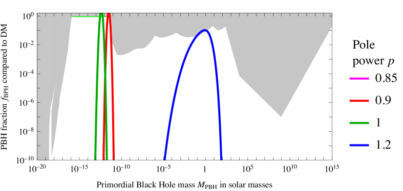
Figure 5: Mass spectra of primordial black holes corresponding to the $P_{\zeta}(k)$ of fig 3 for the indicated pole powers $p$. The normalization is significantly uncertain. The areas shaded in gray are excluded, from [89].

6.2 Primordial Black Holes: results

Fig. 5 shows the PBH mass distributions produced by the sample power spectra of fig 3. The case with $p=0.85$ gives a negligible PBH abundance that does not appear in the plot. For larger $p$ we could choose parameter values such that $P_{\zeta}$ reaches $0.01$, saturating the current bounds on the PBH abundance, as indicated by the gray areas in fig. 5.

For $p=0.9$ and $p=1$ we fixed the position of $\phi_{\rm pole}$ in such a way that the generated PBHs fall in the mass range around $10^{-16-12}$ solar masses where PBHs can be all Dark Matter, $f_{\rm PBH}\approx 1$, and the related SIGW are in the range to be explored by LISA.

On the other hand, larger $p$ only allows to generate heavier PBHs. This is because the inflaton remains a larger number $\Delta N$ of $e$-folds around $\phi_{\rm pole}$ after having produced a peak $P_{\zeta}\approx 0.01$. The sample power spectrum for $p=1.2$ generates SIGW around the PTA claim and solar-mass PBH with density around current bounds. PBH with masses below a solar mass could be detected by LIGO/VIRGO, as they would not have astrophysical backgrounds, but these PBHs cannot account for all of the Dark Matter.

Non-Gaussianities are expected to affect both the PBH abundance and the Scalar-Induced Gravitational Waves [90]. A precise inclusion of non-Gaussianities would be interesting because: i) reproducing the PTA observation as SIGW is expected to imply a significant amount of PBH [91]; ii) DM as PBH is expected to imply detectable SIGW. We leave a detailed investigation of the impact on non-Gaussianities for future work.

7 Light particles during inflation

To conclude, we present a possible theory motivation for a kinetic function $K(\phi)$ with a traversable pole or with a dip, as in eq. (5).

A noteworthy aspect of large-field inflation is that the inflaton $\phi$ undergoes a super-Planckian excursion in field space. Thereby, it’s reasonable to consider the possibility that some extra particle(s) with inflaton-dependent masses become light during inflation at some specific value(s) $\phi_{\rm pole}$ of the inflaton field. A simplified model to capture this phenomenon is obtained adding a fermion $\Psi$ with a Yukawa coupling $y$ to the inflaton $\phi$,

$$\mathscr{L}=\frac{(\partial_{\mu}\phi)^{2}}{2}-V(\phi)+\bar{\Psi}(i\not{\partial}-M_{\Psi}-y\phi)\Psi$$ (37)

so that the fermion mass is $\bar{M}_{\Psi}=M_{\Psi}+y\phi$. In string models, extra gauge vectors $V$ with gauge coupling $g$ can similarly become light at special points in moduli field space, $\bar{M}_{V}^{2}=(M_{V}+g\phi)^{2}$ [92]. Extra scalars $S$ tend to behave in a different way, becoming tachionic after crossing $\bar{M}_{S}^{2}=0$, giving rise to ‘water-fall’ inflation. The masses $M_{S,\Psi,V}$ could be of Planck size.

How does the possibility that some extra particle gets massless at $\phi=\phi_{\rm pole}$ affect the inflaton action? Quantum effects due to the light particle can be computed in QFT by expanding the inflaton field as $\phi=\phi_{\rm pole}+\delta\phi$ around the special value $\phi_{\rm pole}$, obtaining

$$\mathscr{L}_{\rm eff}=\frac{K}{2}(\partial_{\mu}\delta\phi)^{2}-\left[V_{0}+T_{0}\,\delta\phi+\frac{m_{0}^{2}}{2}\delta\phi^{2}+A_{0}\,\delta\phi^{3}+\lambda_{0}\,\delta\phi^{4}+\cdots\right]+\cdots.$$ (38)

If the full theory were renormalizable, the expansion in $\delta\phi$ would stop here and be exact. The dominant quantum corrections are log-enhanced and can be computed by solving the usual RG $\beta$ functions for the effective couplings $K,V_{0},T_{0},m_{0}^{2},\ldots$, and promoting them into field-dependent couplings by setting the RG scale $\mu$ to a value comparable to the light particle mass, $\mu\sim y\,\delta\phi=y(\phi-\phi_{\rm pole})$, implying a significant dependence of couplings on $\phi$ around $\phi_{\rm pole}$. The only relevant parameters around $\delta\phi=0$ are $K$ and $V_{0}$, as the higher order terms in $\delta\phi$ (linear, quadratic, cubic, quartic,…) vanish at $\delta\phi=0$.

For the moment we focus on the correction to $K$, ignoring the correction to $V_{0}$. This could be justified in supersymmetric models, where the super-potential does not receive quantum corrections. The fermionic one-loop correction in $4-2\epsilon$ dimensions and dimensional scale $\mu$ multiplies the kinetic term of a $\delta\phi$ scalar with momentum $p$ by

$$K\simeq 1+\gamma\left[\frac{1}{\epsilon}+\ln\frac{\mu^{2}}{\max(\bar{M}_{\Psi}^{2},p^{2})}\right]$$ (39)

where the coefficient $\gamma$ is known as anomalous dimension of $\delta\phi$. The anomalous dimension contributes to the gauge-invariant $\beta$ functions of the couplings, such as $\beta_{\lambda}=4\lambda\gamma+\cdots$ for the scalar quartic. Acceptable large-field inflaton potentials seem to have non-renormalizable form, making convenient to keep $\phi$ non-canonical, $K\neq 1$. The scalar one-loop anomalous dimension is $\gamma=(2y^{2}-Cg^{2})/(4\pi)^{2}$ in a theory with a Yukawa coupling $y$ and a gauge coupling $g$. The coefficient $C$ is gauge-dependent and morally positive, as the corresponding gauge-independent multiplicative terms in the full $\beta$ functions for the renormalizable couplings are positive.

The renormalisation-group resummation of log-enhanced effects promotes the one-loop result of eq. (39) as

$$K_{\rm ren}\simeq 1+\gamma\ln\frac{\mu^{2}}{\delta\phi^{2}}\to\exp\left(\int\gamma\,d\ln\mu^{2}\right)\propto\frac{1}{\delta\phi^{2\gamma}}$$ (40)

for small constant $\gamma$ and small $\delta\phi$. So:

• A Yukawa coupling induces $K>1$ roughly corresponding to eq. (5) with a pole with power $p\simeq 2\gamma>0$ i.e. dimension $d\simeq 1+\gamma$. The extra constant $1$ in eq. (5) accounts for the normal kinetic term, away from the special point $\phi_{\rm pole}$ where extra fermions become light. The parameter $\phi_{*}$ is the field range within which the extra particle is lighter than the inflaton, for order unity couplings $y$.

• A gauge coupling tends to induce $K<1$ roughly corresponding to eq. (5) with a dip, $p<0$. Making the inflaton kinetic term canonical, this is equivalent to add a sudden drop in the inflaton potential. Samples are plotted in fig. 1.

RG equations can be computed in any given particle physics model, possibly motivated by other considerations: the fermions $\Psi$ could be right-handed neutrinos; the vectors $V$ could be U(1)_B-L or SU(5). The large $\gamma\sim 1$ needed to get significant pole effects during inflation needs large couplings $g,y\lesssim\sqrt{4\pi}$. A roughly constant $\gamma$ and thereby a pole-like structure arises if the RG running towards low energies enters an asymptotic safety regime. Banks-Zaks have shown that this can happen in a controllable perturbative regime [93].

7.1 Extra effects

Particles that become temporarily light during inflation generate extra effects, in addition to a quantum correction to the inflaton kinetic function $K(\phi)$.

First, quantum corrections to $V(\phi)$ away from $\phi_{\rm pole}$ can damage the flatness of the inflaton potential.

Second, the vacuum energy $V_{0}$ in eq. (38) is large during inflation and, in a theory with Yukawa couplings $y$ and gauge couplings $g$, $V_{0}$ runs at two loops as

$$\frac{dV_{0}}{d\ln\mu}\sim\frac{g^{4}-y^{4}}{(4\pi)^{4}}V_{0}$$ (42)

This induces an extra feature in the inflaton potential.

Third, in addition to virtual loop effects, particles can be produced during inflation while their mass $\bar{M}(\phi)$ becomes temporarily small as the inflaton evolves in conformal time as $\phi(\tau)$. Fermion production was studied in [95]: simple analytic estimates are obtained assuming that $\bar{M}\ll m_{0}$ is crossed suddenly, in a small proper time $\tau\sim k/\bar{M}^{\prime}$ where $\bar{M}^{\prime}=d\bar{M}/d\tau$. In such a case, the fermion wave-functions $u_{k}(\tau)$ with momentum $k$ are significantly distorted from the free-particle solutions $e^{i\omega_{k}\tau}$ with $\omega_{k}^{2}=k^{2}+a^{2}M^{2}$ up to a maximal momentum $k_{\rm cr}\lesssim\sqrt{\bar{M}^{\prime}}$ that can be larger than $H$. Fermions are next inflated away, giving the number density

$$n(t)\approx\langle\bar{\Psi}\Psi\rangle=n_{*}\,\theta(t-t_{*})e^{-3H(t-t_{*})}\qquad\hbox{where}\qquad\qquad n_{*}\sim k_{\rm cr}^{3}\sim y^{3/2}\dot{\phi}^{3/2}_{*}.$$ (43)

This fermion density back-reacts inducing an extra term in the inflaton equation of motion $\ddot{\phi}+3H\dot{\phi}=-V^{\prime}+y\langle\bar{\Psi}\Psi\rangle$ that reduces $\dot{\phi}$ [95]. Unless fermions decays fast, this real effect should be added to the virtual effects.

8 Discussion and conclusions

In conclusion, we have investigated an inflaton kinetic function $K(\phi)$ featuring a traversable pole. This is equivalent to a finite stretching of the inflaton potential, after transforming the inflaton field into its canonical form. Section 3 presents the formalism for directly computing inflation in the non-canonical basis. Assuming a kinetic function of the form of eq. (5), a pole with power $p<2$ is traversable during inflaton, and can lead to a significantly enhanced power spectrum $P_{\zeta}(k)$ of primordial inhomogeneities at sub-cosmological scales $k$. Consequently, this can lead to observable scalar-induced gravitational waves and to the formation of primordial black holes. Two sub-cases need to be distinguished:

• If $1\leq p<2$ the canonical potential develops an exact inflection point, with vanishing first and second derivatives. This pole is not traversable in slow-roll approximation. Neverthless, a calculation beyond the slow-roll approximation reveals that the pole is classically traversed, provided that its width coefficient is below a critical threshold. A big enhancement of the power spectrum arises if the pole width is tuned to be just below this critical value. The power spectrum grows as $k^{6}$, reaches a peak and next decreases. If $p\gtrsim 1.3$ (depending on the inflaton potential) the decrease is too slow to allow for a significant enhancement of $P_{\zeta}$ up to 0.01.

• If $0<p<1$ the second derivative of the canonical potential diverges at the pole, that remains traversable even within the slow-roll approximation: increasing the coefficient of the pole no longer yields an arbitrarily large enhancement of the power spectrum. Nevertheless, the slow-roll approximation breaks down, a significant enhancement of $P_{\zeta}$ still happens for $p\gtrsim 0.8$ (depending on the inflation potential), with a characteristic different shape of $P_{\zeta}(k)$, and without significantly tuning the model parameters.

Fig. 3 shows example of power spectra.

In section 5 we computed the consequent frequency spectrum $\Omega_{\rm GW}(f)$ of scalar-induced gravitational waves. As depicted in fig. 4 these second-order gravitational waves could reproduce the nHz signal claimed by Pulsar Timing Arrays, or produce signals at higher frequencies. Fig. 4 also illustrates the expected astrophysical foreground, that could act as background.

In section 6 we computed the consequent mass spectrum $f_{\rm PBH}(M)$ of Primordial Black Holes. As illustrated in fig. 5, these PBH can fall in the asteroid-like mass range where PBH can constitute all of Dark Matter. Since the mass of PBH has one-to-one correspondence with the peak of the GW signals, these PBH as DM can be tested via observation of GW peaking in the mHz region, to be explored by LISA. Alternatively, the sample $P_{\zeta}(k)$ that reproduces the Pulsar Timing Arrays anomaly would give heavier PBH, in the testable sub-solar mass range. We neglected non-Gaussian corrections, that should be included in more precise computations of the gravitational-wave spectrum and of the PBH abundance.

Finally, in section 7, we explored a possible theory that gives a pole-like structure in the inflaton kinetic function: quantum corrections originating from Planckian particles with inflaton-dependent mass (such as fermions with a Yukawa coupling to the inflaton) that become light at some specific inflaton vacuum expectation value. In such a case the pole power $p$ is related to the quantum anomalous dimension of the inflaton. This might give single-field inflation theories with enhanced $P_{\zeta}$ and mild tuning. However, as discussed, this theoretical approach tends to introduce additional effects beyond the mere presence of the pole: dedicated future computations are needed to clarify. Multiple poles might arise at different values of the inflaton vacuum expectation values, corresponding to different particles becoming light. In such a case the power spectrum and the consequent gravitational wave spectrum could exhibit multiple peaks. If future experiments will advance gravitational wave astronomy, the detection of such signals could provide insights into Planckian physics.

Acknowledgements

We thank Michele Redi and Sotirios Karamitsos for useful discussions.

References

- [1] R. Kallosh, A. Linde, D. Roest, JHEP 08 (2014) 052 [\IfSubStr1405.3646:InSpire:1405.3646arXiv:1405.3646].
- [2] J.J.M. Carrasco, R. Kallosh, A. Linde, Phys.Rev.D 92 (2015) 063519 [\IfSubStr1506.00936:InSpire:1506.00936arXiv:1506.00936].
- [3] M. Rinaldi, L. Vanzo, S. Zerbini, G. Venturi, Phys.Rev.D 93 (2016) 024040 [\IfSubStr1505.03386:InSpire:1505.03386arXiv:1505.03386].
- [4] K. Dimopoulos, C. Owen, JCAP 06 (2017) 027 [\IfSubStr1703.00305:InSpire:1703.00305arXiv:1703.00305].
- [5] S. Karamitsos, A. Strumia, JHEP 05 (2022) 016 [\IfSubStr2109.10367:InSpire:2109.10367arXiv:2109.10367].
- [6] P. Ivanov, P. Naselsky, I. Novikov, Phys.Rev.D 50 (1994) 7173.
- [7] W.H. Kinney, Phys.Rev.D 72 (2005) 023515 [\IfSubStrgr-qc/0503017:InSpire:gr-qc/0503017arXiv:gr-qc/0503017].
- [8] G. Ballesteros, C. Tamarit, JHEP 02 (2016) 153 [\IfSubStr1510.05669:InSpire:1510.05669arXiv:1510.05669].
- [9] N. Okada, D. Raut, Phys.Rev.D 95 (2017) 035035 [\IfSubStr1610.09362:InSpire:1610.09362arXiv:1610.09362].
- [10] K. Kannike, L. Marzola, M. Raidal, H. Veermäe, JCAP 09 (2017) 020 [\IfSubStr1705.06225:InSpire:1705.06225arXiv:1705.06225].
- [11] C. Germani, T. Prokopec, Phys.Dark Univ. 18 (2017) 6 [\IfSubStr1706.04226:InSpire:1706.04226arXiv:1706.04226].
- [12] F. Bezrukov, M. Pauly, J. Rubio, JCAP 02 (2018) 040 [\IfSubStr1706.05007:InSpire:1706.05007arXiv:1706.05007].
- [13] G. Ballesteros, M. Taoso, Phys.Rev.D 97 (2018) 023501 [\IfSubStr1709.05565:InSpire:1709.05565arXiv:1709.05565].
- [14] M.P. Hertzberg, M. Yamada, Phys.Rev.D 97 (2018) 083509 [\IfSubStr1712.09750:InSpire:1712.09750arXiv:1712.09750].
- [15] J.M. Ezquiaga, J. García-Bellido, JCAP 08 (2018) 018 [\IfSubStr1805.06731:InSpire:1805.06731arXiv:1805.06731].
- [16] I. Dalianis, A. Kehagias, G. Tringas, JCAP 01 (2019) 037 [\IfSubStr1805.09483:InSpire:1805.09483arXiv:1805.09483].
- [17] S. Rasanen, E. Tomberg, JCAP 01 (2019) 038 [\IfSubStr1810.12608:InSpire:1810.12608arXiv:1810.12608].
- [18] S.-L. Cheng, W. Lee, K.-W. Ng, Phys.Rev.D 99 (2019) 063524 [\IfSubStr1811.10108:InSpire:1811.10108arXiv:1811.10108].
- [19] M. Drees, Y. Xu, Eur.Phys.J.C 81 (2021) 182 [\IfSubStr1905.13581:InSpire:1905.13581arXiv:1905.13581].
- [20] R. Mahbub, Phys.Rev.D 101 (2020) 023533 [\IfSubStr1910.10602:InSpire:1910.10602arXiv:1910.10602].
- [21] J. Lin, Q. Gao, Y. Gong, Y. Lu, C. Zhang, F. Zhang, Phys.Rev.D 101 (2020) 103515 [\IfSubStr2001.05909:InSpire:2001.05909arXiv:2001.05909].
- [22] J. Lin, S. Gao, Y. Gong, Y. Lu, Z. Wang, F. Zhang, Phys.Rev.D 107 (2023) 043517 [\IfSubStr2111.01362:InSpire:2111.01362arXiv:2111.01362].
- [23] D. Frolovsky, S.V. Ketov, S. Saburov, Frontiers in Phys. 10 (2022) 1005333 [\IfSubStr2207.11878:InSpire:2207.11878arXiv:2207.11878].
- [24] A. Ghoshal, A. Moursy, Q. Shafi, Phys.Rev.D 108 (2023) 055039 [\IfSubStr2306.04002:InSpire:2306.04002arXiv:2306.04002].
- [25] C. Chen, A. Ghoshal, Z. Lalak, Y. Luo, A. Naskar, JCAP 08 (2023) 041 [\IfSubStr2305.12325:InSpire:2305.12325arXiv:2305.12325].
- [26] S.-M. Choi, H.M. Lee, Eur.Phys.J.C 76 (2016) 303 [\IfSubStr1601.05979:InSpire:1601.05979arXiv:1601.05979].
- [27] M. Drees, Y. Xu, JCAP 09 (2021) 012 [\IfSubStr2104.03977:InSpire:2104.03977arXiv:2104.03977].
- [28] A.A. Starobinsky, JETP Lett. 55 (1992) 489. J.A. Adams, B. Cresswell, R. Easther, Phys.Rev.D 64 (2001) 123514 [\IfSubStrastro-ph/0102236:InSpire:astro-ph/0102236arXiv:astro-ph/0102236]. K. Kefala, G.P. Kodaxis, I.D. Stamou, N. Tetradis, Phys.Rev.D 104 (2021) 023506 [\IfSubStr2010.12483:InSpire:2010.12483arXiv:2010.12483]. K. Inomata, E. McDonough, W. Hu, JCAP 02 (2022) 031 [\IfSubStr2110.14641:InSpire:2110.14641arXiv:2110.14641].
- [29] K. Inomata, E. McDonough, W. Hu, Phys.Rev.D 104 (2021) 123553 [\IfSubStr2104.03972:InSpire:2104.03972arXiv:2104.03972].
- [30] Planck Collaboration, Astron.Astrophys. 641 (2020) A10 [\IfSubStr1807.06211:InSpire:1807.06211arXiv:1807.06211]. BICEP, Keck Collaborations, Phys.Rev.Lett. 127 (2021) 151301 [\IfSubStr2110.00483:InSpire:2110.00483arXiv:2110.00483].
- [31] D. Burns, S. Karamitsos, A. Pilaftsis, Nucl.Phys.B 907 (2016) 785 [\IfSubStr1603.03730:InSpire:1603.03730arXiv:1603.03730].
- [32] S. Karamitsos, A. Pilaftsis, Nucl.Phys.B 927 (2018) 219 [\IfSubStr1706.07011:InSpire:1706.07011arXiv:1706.07011].
- [33] X. Chen, M.-. Huang, S. Kachru, G. Shiu, JCAP 01 (2007) 002 [\IfSubStrhep-th/0605045:InSpire:hep-th/0605045arXiv:hep-th/0605045].
- [34] A.A. Starobinsky, Phys.Lett.B 91 (1980) 99.
- [35] F.L. Bezrukov, M. Shaposhnikov, Phys.Lett.B 659 (2008) 703 [\IfSubStr0710.3755:InSpire:0710.3755arXiv:0710.3755].
- [36] P.S. Cole, A.D. Gow, C.T. Byrnes, S.P. Patil, JCAP 08 (2023) 031 [\IfSubStr2304.01997:InSpire:2304.01997arXiv:2304.01997].
- [37] D.J. Fixsen, E.S. Cheng, J.M. Gales, J.C. Mather, R.A. Shafer, E.L. Wright, Astrophys.J. 473 (1996) 576 [\IfSubStrastro-ph/9605054:InSpire:astro-ph/9605054arXiv:astro-ph/9605054].
- [38] K. Inomata, M. Kawasaki, Y. Tada, Phys.Rev.D 94 (2016) 043527 [\IfSubStr1605.04646:InSpire:1605.04646arXiv:1605.04646].
- [39] PIXIE Collaboration, JCAP 07 (2011) 025 [\IfSubStr1105.2044:InSpire:1105.2044arXiv:1105.2044].
- [40] J. Chluba, A.L. Erickcek, I. Ben-Dayan, Astrophys.J. 758 (2012) 76 [\IfSubStr1203.2681:InSpire:1203.2681arXiv:1203.2681].
- [41] A. Ghoshal, Z. Lalak, S. Porey, Phys.Rev.D 108 (2023) 063030 [\IfSubStr2302.03268:InSpire:2302.03268arXiv:2302.03268].
- [42] I. Stamou, S. Clesse [\IfSubStr2310.04174:InSpire:2310.04174arXiv:2310.04174].
- [43] O. Özsoy, G. Tasinato, Universe 9 (2023) 203 [\IfSubStr2301.03600:InSpire:2301.03600arXiv:2301.03600].
- [44] K.N. Ananda, C. Clarkson, D. Wands, Phys.Rev.D 75 (2007) 123518 [\IfSubStrgr-qc/0612013:InSpire:gr-qc/0612013arXiv:gr-qc/0612013].
- [45] D. Baumann, P.J. Steinhardt, K. Takahashi, K. Ichiki, Phys.Rev.D 76 (2007) 084019 [\IfSubStrhep-th/0703290:InSpire:hep-th/0703290arXiv:hep-th/0703290].
- [46] K. Kohri, T. Terada, Phys.Rev.D 97 (2018) 123532 [\IfSubStr1804.08577:InSpire:1804.08577arXiv:1804.08577].
- [47] M. Sasaki, T. Suyama, T. Tanaka, S. Yokoyama, Class.Quant.Grav. 35 (2018) 063001 [\IfSubStr1801.05235:InSpire:1801.05235arXiv:1801.05235].
- [48] G. Domènech, Universe 7 (2021) 398 [\IfSubStr2109.01398:InSpire:2109.01398arXiv:2109.01398].
- [49] A. Escrivà, F. Kuhnel, Y. Tada [\IfSubStr2211.05767:InSpire:2211.05767arXiv:2211.05767].
- [50] K.N. Ananda, C. Clarkson, D. Wands, Phys.Rev.D 75 (2007) 123518 [\IfSubStrgr-qc/0612013:InSpire:gr-qc/0612013arXiv:gr-qc/0612013].
- [51] D.H. Lyth, A. Riotto, Phys.Rept. 314 (1999) 1 [\IfSubStrhep-ph/9807278:InSpire:hep-ph/9807278arXiv:hep-ph/9807278].
- [52] J.R. Espinosa, D. Racco, A. Riotto, JCAP 09 (2018) 012 [\IfSubStr1804.07732:InSpire:1804.07732arXiv:1804.07732].
- [53] D.R. Brill, J.B. Hartle, Phys.Rev. 135 (1964) B271.
- [54] R.A. Isaacson, Phys.Rev. 166 (1968) 1263.
- [55] R.A. Isaacson, Phys.Rev. 166 (1968) 1272.
- [56] L.H. Ford, L. Parker, Phys.Rev.D 16 (1977) 1601.
- [57] A. Ota, H.J. Macpherson, W.R. Coulton, Phys.Rev.D 106 (2022) 063521 [\IfSubStr2111.09163:InSpire:2111.09163arXiv:2111.09163].
- [58] NanoGrav Collaboration [\IfSubStr2306.16213:InSpire:2306.16213arXiv:2306.16213]. PPTA Collaboration [\IfSubStr2306.16215:InSpire:2306.16215arXiv:2306.16215]. EPTA Collaboration [\IfSubStr2306.16214:InSpire:2306.16214arXiv:2306.16214]. CPTA Collaboration [\IfSubStr2306.16216:InSpire:2306.16216arXiv:2306.16216].
- [59] M. Maggiore, Phys.Rept. 331 (2000) 283 [\IfSubStrgr-qc/9909001:InSpire:gr-qc/9909001arXiv:gr-qc/9909001].
- [60] Planck Collaboration, Astron.Astrophys. 641 (2020) A6 [\IfSubStr1807.06209:InSpire:1807.06209arXiv:1807.06209].
- [61] CMB-HD Collaboration [\IfSubStr2203.05728:InSpire:2203.05728arXiv:2203.05728].
- [62] LIGO, Virgo Collaborations, Phys.Rev.Lett. 116 (2016) 061102 [\IfSubStr1602.03837:InSpire:1602.03837arXiv:1602.03837]. LIGO, Virgo Collaborations, Astrophys.J.Lett. 851 (2017) L35 [\IfSubStr1711.05578:InSpire:1711.05578arXiv:1711.05578]. LIGO, Virgo Collaborations, Phys.Rev.Lett. 119 (2017) 161101 [\IfSubStr1710.05832:InSpire:1710.05832arXiv:1710.05832].
- [63] VIRGO Collaboration, Class.Quant.Grav. 32 (2015) 024001 [\IfSubStr1408.3978:InSpire:1408.3978arXiv:1408.3978].
- [64] LIGO, Virgo Collaborations, SoftwareX 13 (2021) 100658 [\IfSubStr1912.11716:InSpire:1912.11716arXiv:1912.11716].
- [65] S. Hild et al., Class.Quant.Grav. 28 (2011) 094013 [\IfSubStr1012.0908:InSpire:1012.0908arXiv:1012.0908].
- [66] LISA Collaboration [\IfSubStr1907.06482:InSpire:1907.06482arXiv:1907.06482].
- [67] DECIGO Collaboration, Class.Quant.Grav. 28 (2011) 094011.
- [68] A. Sesana et al., Exper.Astron. 51 (2021) 1333 [\IfSubStr1908.11391:InSpire:1908.11391arXiv:1908.11391].
- [69] SKA Collaboration, Publ.Astron.Soc.Austral. 37 (2020) e002 [\IfSubStr1810.02680:InSpire:1810.02680arXiv:1810.02680].
- [70] J. Garcia-Bellido, H. Murayama, G. White, JCAP 12 (2021) 023 [\IfSubStr2104.04778:InSpire:2104.04778arXiv:2104.04778].
- [71] LIGO, Virgo Collaborations, Phys.Rev.D 93 (2016) 122003 [\IfSubStr1602.03839:InSpire:1602.03839arXiv:1602.03839]. LIGO, Virgo Collaborations, Phys.Rev.X 6 (2016) 041015 [\IfSubStr1606.04856:InSpire:1606.04856arXiv:1606.04856]. LIGO, Virgo Collaborations, Phys.Rev.X 9 (2019) 031040 [\IfSubStr1811.12907:InSpire:1811.12907arXiv:1811.12907].
- [72] LIGO, Virgo Collaborations, Phys.Rev.Lett. 120 (2018) 091101 [\IfSubStr1710.05837:InSpire:1710.05837arXiv:1710.05837].
- [73] C. Cutler, J. Harms, Phys.Rev.D 73 (2006) 042001 [\IfSubStrgr-qc/0511092:InSpire:gr-qc/0511092arXiv:gr-qc/0511092].
- [74] T. Regimbau, M. Evans, N. Christensen, E. Katsavounidis, B. Sathyaprakash, S. Vitale, Phys.Rev.Lett. 118 (2017) 151105 [\IfSubStr1611.08943:InSpire:1611.08943arXiv:1611.08943].
- [75] A.J. Farmer, E.S. Phinney, Mon. Not. Roy. Astron. Soc. 346 (2003) 1197 [\IfSubStrastro-ph/0304393:InSpire:astro-ph/0304393arXiv:astro-ph/0304393].
- [76] P.A. Rosado, Phys.Rev.D 84 (2011) 084004 [\IfSubStr1106.5795:InSpire:1106.5795arXiv:1106.5795].
- [77] C.J. Moore, R.H. Cole, C.P.L. Berry, Class.Quant.Grav. 32 (2015) 015014 [\IfSubStr1408.0740:InSpire:1408.0740arXiv:1408.0740].
- [78] M.R. Adams, N.J. Cornish, Phys.Rev.D 82 (2010) 022002 [\IfSubStr1002.1291:InSpire:1002.1291arXiv:1002.1291].
- [79] M.R. Adams, N.J. Cornish, Phys.Rev.D 89 (2014) 022001 [\IfSubStr1307.4116:InSpire:1307.4116arXiv:1307.4116].
- [80] X.-J. Zhu, E.J. Howell, D.G. Blair, Z.-H. Zhu, Mon.Not.Roy.Astron.Soc. 431 (2013) 882 [\IfSubStr1209.0595:InSpire:1209.0595arXiv:1209.0595].
- [81] W.H. Press, P. Schechter, Astrophys.J. 187 (1974) 425.
- [82] I. Musco, J.C. Miller, L. Rezzolla, Class.Quant.Grav. 22 (2005) 1405 [\IfSubStrgr-qc/0412063:InSpire:gr-qc/0412063arXiv:gr-qc/0412063].
- [83] I. Musco, V. De Luca, G. Franciolini, A. Riotto, Phys.Rev.D 103 (2021) 063538 [\IfSubStr2011.03014:InSpire:2011.03014arXiv:2011.03014].
- [84] B.J. Carr, Astrophys.J. 201 (1975) 1.
- [85] K. Jedamzik, J.C. Niemeyer, Phys.Rev.D 59 (1999) 124014 [\IfSubStrastro-ph/9901293:InSpire:astro-ph/9901293arXiv:astro-ph/9901293].
- [86] G. Franciolini, A. Kehagias, S. Matarrese, A. Riotto, JCAP 03 (2018) 016 [\IfSubStr1801.09415:InSpire:1801.09415arXiv:1801.09415].
- [87] V. Atal, C. Germani, Phys.Dark Univ. 24 (2019) 100275 [\IfSubStr1811.07857:InSpire:1811.07857arXiv:1811.07857].
- [88] G. Ferrante, G. Franciolini, G. Franciolini, A. Urbano, Phys.Rev.D 107 (2023) 043520 [\IfSubStr2211.01728:InSpire:2211.01728arXiv:2211.01728].
- [89] M. Cirelli, A. Strumia, J. Zupan, “Dark Matter”, to appear.
- [90] R. Cai, S. Pi, M. Sasaki, Phys.Rev.Lett. 122 (2019) 201101 [\IfSubStr1810.11000:InSpire:1810.11000arXiv:1810.11000]. C. Unal, Phys.Rev.D 99 (2019) 041301 [\IfSubStr1811.09151:InSpire:1811.09151arXiv:1811.09151]. P. Adshead, K.D. Lozanov, Z.J. Weiner, JCAP 10 (2021) 080 [\IfSubStr2105.01659:InSpire:2105.01659arXiv:2105.01659].
- [91] G. Franciolini, G. Franciolini, V. Vaskonen, H. Veermae [\IfSubStr2306.17149:InSpire:2306.17149arXiv:2306.17149].
- [92] L.E. Ibanez, W. Lerche, D. Lust, S. Theisen, Nucl.Phys.B 352 (1991) 435.
- [93] T. Banks, A. Zaks, Nucl.Phys.B 196 (1982) 189.
- [94] S.P. Martin, Phys.Rev.D 96 (2017) 096005 [\IfSubStr1709.02397:InSpire:1709.02397arXiv:1709.02397].
- [95] D.J.H. Chung, E.W. Kolb, A. Riotto, I.I. Tkachev, Phys.Rev.D 62 (2000) 043508 [\IfSubStrhep-ph/9910437:InSpire:hep-ph/9910437arXiv:hep-ph/9910437].
- [96] H. Di, Y. Gong, JCAP 07 (2018) 007 [\IfSubStr1707.09578:InSpire:1707.09578arXiv:1707.09578].
- [97] R.L. Arnowitt, S. Deser, C.W. Misner, Gen.Rel.Grav. 40 (2008) 1997 [\IfSubStrgr-qc/0405109:InSpire:gr-qc/0405109arXiv:gr-qc/0405109].
- [98] J.M. Maldacena, JHEP 05 (2003) 013 [\IfSubStrastro-ph/0210603:InSpire:astro-ph/0210603arXiv:astro-ph/0210603].
- [99] D. Seery, J.E. Lidsey, JCAP 06 (2005) 003 [\IfSubStrastro-ph/0503692:InSpire:astro-ph/0503692arXiv:astro-ph/0503692].