Entanglement of Gauge Theories: from the Toric Code to the $\mathbb{Z}_{2}$ Lattice Gauge Higgs Model

Abstract

The toric code (TC) model subjected to a magnetic field can be mapped to the $\mathbb{Z}_{2}$ lattice gauge Higgs ($\mathbb{Z}_{2}$ GH) model. Although this isometric mapping preserves the bulk energy spectrum, here, we show that it has a non-trivial effect on the entanglement structure. We derive a quantum channel that allows us to obtain the reduced density matrix of the $\mathbb{Z}_{2}$ GH model from the one of the TC model. We then contrast the ground state entanglement spectra (ES) of the two models. Analyzing the role of the electric-magnetic duality, we show that while the ES of the TC model is enriched by the duality, the ES of the $\mathbb{Z}_{2}$ GH model is in fact not. This thus represents an example where the bulk-boundary correspondence fails. Moreover, the quantum channel allows us to investigate the entanglement distillation of the $\mathbb{Z}_{2}$ GH model from the TC model.

Introduction. Entanglement plays an essential role in understanding and characterizing quantum many-body systems [1]. Notably, intrinsic topological order [2] is characterized by its long-range entanglement and the resulting topological entanglement entropy [3, 4]. The entanglement spectrum (ES) [5], i.e., the (negative logarithmic) spectrum of the reduced density matrix, has been proposed to provide additional information about the structure of entanglement in topological phases of matter.

One of the most celebrated models with an intrinsic topologically ordered ground state is the toric code (TC) model [6, 7]. The TC model in presence of a magnetic field can be mapped by an isometry to another fundamental model, the $\mathbb{Z}_{2}$ lattice gauge Higgs ($\mathbb{Z}_{2}$ GH) model [8, 9, 10, 11]—a simple lattice gauge theory realizing Higgs and confinement transitions. Therefore, the TC model and the $\mathbb{Z}_{2}$ GH model have an identical bulk energy spectrum. However, in this work, we show that the isometric mapping between the two models changes the entanglement structure in a non-trivial way, giving rise to several questions: First, while Ref. [12] showed that the electric-magnetic duality symmetry can enrich the ES of a $\mathbb{Z}_{2}$ topological state, it is not clear how the duality symmetry affects the ES of the $\mathbb{Z}_{2}$ GH model. Second, Ref. [13] points out an interesting boundary transition of the $\mathbb{Z}_{2}$ GH model and it is not clear whether the ES reflects the boundary physics according to a bulk-boundary correspondence. Third, a main difference between the TC model and the $\mathbb{Z}_{2}$ GH model is that the Hilbert space of the latter has a gauge constraint. Several works study the entanglement entropy by taking the gauge constraint into consideration [14, 15, 16, 17, 18, 19, 20], and some conjectures have been proposed which deserve further investigation [15].

In this work, we derive a quantum channel that allows us to directly obtain the reduced density matrices of the $\mathbb{Z}_{2}$ GH model from the reduced density matrix of the TC model and to explain the differences and similarities of their ES. Using the quantum channel, we can then understand how symmetry applies to the reduced density matrix of the $\mathbb{Z}_{2}$ GH model and explain their consequences on the ES. By combining the quantum channel and tensor network methods, we derive an efficient approach to extract the ES and entanglement entropy of the $\mathbb{Z}_{2}$ GH model from the solution of the TC model.

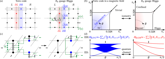
Figure 1: Entanglement structure of the TC and $\mathbb{Z}_{2}$ GH model. (a) The TC and $\mathbb{Z}_{2}$ GH model are defined on a square lattice. The TC model consists of qubits on the edges (dots). In the $\mathbb{Z}_{2}$ GH model, the qubits on edges (vertices) are the $\mathbb{Z}_{2}$ gauge (matter) fields with local gauge constraints $X_{v}A_{v}=1$. The entanglement bipartitions cut the systems into left (right) part $L$ ($R$), where $\partial L\subset L$ ($\partial R\subset R$) are the boundaries of $L$ ($R$). (b) Schematic phase diagrams of the TC and the $\mathbb{Z}_{2}$ GH model. (c) For a small subsystem [dotted box in (a)] we illustrate the transformation of the reduced TC density matrix $\rho_{\text{TC}}$ to the reduced $\mathbb{Z}_{2}$ GH density matrix $\rho_{\text{GH}}$ by the CX gates in the isometry $V$ (only horizontal gates are shown). By tracing the $L$ part, the CX gates that are entirely in the $L$ part cancel each other. Those that cross the entanglement cut and those that are in the $R$ part form the quantum channel $\mathscr{N}[\cdot]$. (d) The entanglement Hamiltonian (EH) for the TC ($\mathbb{Z}_{2}$ GH) model along the black dotted lines in (b) is approximated by a quantum (classical) Ising chain projected to the even $\mathbb{Z}_{2}$ parity sector, where $P_{+}=(1+\prod_{i}Z_{i})/2$.

Definition of the TC and $\mathbb{Z}_{2}$ GH model. The TC model is defined on a square lattice with qubits on the edges as shown in Fig. 1a. We label the edges, vertices, and plaquettes of the lattice as $e$, $v$, and $p$, respectively. The Hamiltonian of the TC model in a magnetic field is given by

$$H_{\text{TC}}=-\sum_{v}A_{v}-\sum_{p}B_{p}-h_{x}\sum_{e}X_{e}-h_{z}\sum_{e}Z_{e},$$ (1)

where $A_{v}=\prod_{e\in v}X_{e}$ and $B_{p}=\prod_{e\in p}Z_{e}$ are vertex and plaquette operators and $X_{e}$ and $Z_{e}$ are Pauli matrices. In the following, we will use a parameterization in polar coordinates $(h,\theta)=\left(\sqrt{h_{x}^{2}+h_{z}^{2}},\text{arctan}(h_{x}/h_{z})\right)$, where $h$ ($\theta$) is the strength (direction) of the magnetic field. The phase diagram of the model [21, 22], exhibiting a toric code phase with the $\mathbb{Z}_{2}$ topological order and a trivial phase, is shown in Fig. 1b. The phase diagram is symmetric about $\theta=\pi/4$ due to the electric-magnetic duality symmetry, $U_{\text{TC}}H_{\text{TC}}(h_{x},h_{z})U^{\dagger}_{\text{TC}}=H_{\text{TC}}(h_{z},h_{x})$, where $U_{\text{TC}}$ is the duality transformation exchanging the primal lattice and the dual lattice as well as $X$ and $Z$.

It is established that the TC model can be exactly transformed to the $\mathbb{Z}_{2}$ GH model  [8]. The Hilbert space of the $\mathbb{Z}_{2}$ GH model consists of $\mathbb{Z}_{2}$ gauge (matter) field on edges (vertices) of the lattice. The mapping between the two models is given by the isometry

$$V=\prod_{\langle e,v\rangle}\text{CX}_{v,e}\prod_{v}\ket{+}_{v},$$ (2)

where $\text{CX}_{v,e}=X_{e}^{(1-Z_{v})/2}$ is the controlled-X gate acting on a controlling qubit $v$ and a nearest-neighbor controlled qubit $e$. Applying $V$ on $H_{\text{TC}}$ yields the Hamiltonian of the $\mathbb{Z}_{2}$ GH model: $H_{\text{GH}}=VH_{\text{TC}}V^{\dagger}$, which can be explicitly expressed as

$$H_{\text{GH}}=-\sum_{v}X_{v}-\sum_{p}B_{p}-h_{x}\sum_{e}X_{e}-h_{z}\sum_{e}Z_{v(e)}Z_{e}Z_{v^{\prime}(e)},$$ (3)

where $v(e)$ and $v^{\prime}(e)$ are two vertices which are closest to the edge $e$ (see Fig. 1a) and $h_{z}$ ($h_{x}$) can be regarded as the strength of the gauge-matter coupling (gauge fluctuations). Since $V^{\dagger}V=\mathbbm{1}$ and $VV^{\dagger}=\prod_{v}[(1+X_{v}A_{v})/2]$, the Hilbert space of the $\mathbb{Z}_{2}$ GH model has to satisfy the gauge constraint $X_{v}A_{v}=1,\forall v$, representing Gauss law. The ground states $\ket{\Psi_{\text{GH}}}$ of the $\mathbb{Z}_{2}$ GH model can thus be obtained from the ground states $\ket{\Psi_{\text{TC}}}$ of the TC model as $\ket{\Psi_{\text{GH}}}=V\ket{\Psi_{\text{TC}}}$. For $h_{z}=0$, the model reduces to a pure $\mathbb{Z}_{2}$ gauge model in which the gauge and matter fields are not entangled, i.e., $\ket{\Psi_{\text{GH}}}=\ket{\Psi_{\text{TC}}}\otimes\prod_{v}\ket{+}_{v}$.

Since the isometry $V$ preserves the bulk energy spectrum, the phase diagrams of the two models are the same; Fig. 1b. The deconfined phase of the $\mathbb{Z}_{2}$ GH model corresponds to the toric code phase. At sufficiently large fields, a phase transition to the Higgs (confining) phase occurs in which $\mathbb{Z}_{2}$ charges condense (are confined). The Higgs and the confined phase are adiabatically connected and thus they are the same phase [11]. Moreover, as the phase diagram is symmetric about $\theta=\pi/4$, there is a modified duality $U_{\text{GH}}=VU_{\text{TC}}V^{\dagger}$ of the $\mathbb{Z}_{2}$ GH model: $U_{\text{GH}}H_{\text{GH}}(h_{x},h_{z})U_{\text{GH}}^{\dagger}=H_{\text{GH}}(h_{z},h_{x})$.

Quantum channel. Starting from a quantum state $\ket{\Psi_{\text{TC}}}$ defined in the Hilbert space of the TC model, the reduced density matrix $\rho_{\text{TC}}=\Tr_{L}\ket{\Psi_{\text{TC}}}\bra{\Psi_{\text{TC}}}$ is obtained by tracing the degrees of freedom in the left part $L$ of the system on an infinitely long cylinder with a circumference $N$, see Fig 1a. The corresponding quantum state in the Hilbert space of the $\mathbb{Z}_{2}$ GH model is $\ket{\Psi_{\text{GH}}}=V\ket{\Psi_{\text{TC}}}$, from which the reduced density matrix $\rho_{\text{GH}}=\Tr_{L}\ket{\Psi_{\text{GH}}}\bra{\Psi_{\text{GH}}}$ is obtained.

As shown in Fig. 1c, we can derive the transformation $\mathscr{N}[\cdot]$ relating the reduced density matrices $\rho_{\text{TC}}$ and $\rho_{\text{GH}}$ from the isometric transformation $V$ in Eq. (2) such that

$$\rho_{\text{GH}}=\mathscr{N}[\rho_{\text{TC}}]=\sum_{\boldsymbol{z}}K_{\boldsymbol{z}}\rho_{\text{TC}}K^{\dagger}_{\boldsymbol{z}},$$ (4)

where $\ket{\boldsymbol{z}}=\prod_{v\in\partial L}\ket{z_{v}}_{v}$ and $z=0$ or $1$, and the Kraus operators

$$K_{\boldsymbol{z}}=\frac{1}{2^{N/2}}\prod_{\langle e\in R,v\in R\cup\partial L\rangle}\text{CX}_{v,e}\ket{\boldsymbol{z}}\otimes\prod_{v\in R}\ket{+}_{v}.$$ (5)

The map $\mathscr{N}[\cdot]$ satisfies the trace-preserving condition (i.e., $\sum_{\boldsymbol{z}}K_{\boldsymbol{z}}^{\dagger}K_{\boldsymbol{z}}=\mathbbm{1}$) and it maps the identity operator to a projector (i.e., $\sum_{\boldsymbol{z}}K_{\boldsymbol{z}}K_{\boldsymbol{z}}^{\dagger}=\prod_{v\in R}[(1+X_{v}A_{v})/2]$). Thus $\mathscr{N}[\cdot]$ is a quantum channel; see supplemental material [23]. In the subspace satisfying the gauge constraint, the projector is equivalent to an identity operator, so $\mathscr{N}[\cdot]$ satisfies the unital condition (map $\mathbbm{1}$ to $\mathbbm{1}$). Since the quantum channel does not necessarily preserve the spectrum of a density matrix, the ES of the $\mathbb{Z}_{2}$ GH model is generically different from that of the TC model. There are some additional properties of the quantum channel $\mathscr{N}[\cdot]$ [23], which are useful for contrasting the entanglement of the TC model and the $\mathbb{Z}_{2}$ GH model and for studying the entanglement structures of the $\mathbb{Z}_{2}$ GH model: (i) The quantum channel has a gauge symmetry $[\mathscr{N}[\cdot],X_{e}]=0,\forall e\in\partial R$, and satisfies the gauge constraint $X_{v}A_{v}\mathscr{N}[\cdot]=\mathscr{N}[\cdot]X_{v}A_{v}=\mathscr{N}[\cdot],\forall v\in R$. (ii) If $\exists e\in\partial R$, such that $\{O,X_{e}\}=0$, then $\mathscr{N}[O]=0$. (iii) For operators $O$ satisfying the gauge symmetry $[O,X_{e}]=0,\forall e\in\partial R$ and the gauge constraint $OX_{v}A_{v}=X_{v}A_{v}O=O,\forall v\in R$, there exists an map $\mathscr{N}^{-1}[\cdot]=\sum_{\boldsymbol{z}}K^{\dagger}_{\boldsymbol{z}}\cdot K_{\boldsymbol{z}}$ such that $\mathscr{N}[\mathscr{N}^{-1}[O]]=O$.

Entanglement Hamiltonian and ES of the TC model. In the toric code phase, the ground states has a fourfold topological degeneracy for the infinite cylinder geometry represented by so-called minimally entangled states (MES) [24]. For simplicity, we only consider the trivial MES corresponding to the vacuum sector . When the magnetic field strength $h$ is small, the ground state can be approximated by perturbation theory $\ket{\Psi_{\text{TC}}}=\left[1+\frac{h_{x}}{4}\sum_{e}X_{e}+\frac{h_{z}}{4}\sum_{e}Z_{e}+O(h^{2})\right]\ket{\text{TC}}$, where $\ket{\text{TC}}$ is the trivial MES at $h=0$. From $\ket{\Psi_{\text{TC}}}$, the entanglement Hamiltonian is obtained as $H_{E,\text{TC}}=-\log(\rho_{\text{TC}})$. Since we are interested in the low-energy degrees of freedom, we use an isometry $\mathcal{V}_{\text{TC}}$ to transform the $H_{E,\text{TC}}$ into the effective Hamiltonian $\tilde{H}_{E,\text{TC}}=\mathcal{V}_{\text{TC}}H_{E,\text{TC}}\mathcal{V}^{\dagger}_{\text{TC}}+O(h^{2})$ [26] by discarding the high-energy part. In fact, only the terms $\sum_{e\in\partial R}X_{e}$ and $\sum_{e\in\partial L}Z_{e}$ in $\ket{\Psi_{\text{TC}}}$ contribute to first order $O(h)$ of $\tilde{H}_{E,\text{TC}}$, where $\partial L$ ($\partial R$) is a set of edges at the boundary of region $L$ ($R$) and these terms become $\sum_{i}X_{i}X_{i+1}$ and $\sum_{i}Z_{i}$ in $\tilde{H}_{E,\text{TC}}$. Taking the projector $P_{+}=(1\pm\prod_{i}Z_{i})/2$ (defined in the Hilbert subspace of $\tilde{H}_{E,\text{TC}}$) to the trivial MES into consideration, we derive the effective entanglement Hamiltonian [23],

$$\tilde{H}_{E,\text{TC}}=P_{+}\left[\log 2^{N-1}-\sum_{i=1}^{N}\left(\frac{h_{z}}{2}Z_{i}+\frac{h_{x}}{2}X_{i}X_{i+1}\right)+O(h^{2})\right].$$ (6)

By contrast, in the limit $h\rightarrow\infty$, the ground state of the TC model becomes a product state, whose effective entanglement Hamiltonian is a $1\times 1$ dimensional matrix: $\tilde{H}_{E,\text{TC}}=0$.

Next we use tensor-network methods to calculate the ES, i.e., the energy spectrum $\{\epsilon_{i}\}$ of $H_{E}$. We first approximate the ground state of the TC model by variationally optimizing an infinite 2D tensor network ansatz, the infinite projected entangled pair states (iPEPS) [27, 28, 29]. There are two important parameters that systematically control the error of the approximation; the bond dimension $D$ of the iPEPS itself and the bond dimension $\chi$ of the boundary infinite matrix product operator (iMPO) used to contract the iPEPS [23]. We then calculate the ES on an infinitely long cylinder with a finite circumference from the iMPO [26]. The ES of the trivial MES in the topologically ordered phase at a small magnetic field $h=0.02$ is shown in Fig. 2a. From perturbation theory, the entanglement Hamiltonian has a transition at $\theta=\pi/4$ described by the Ising conformal field theory (CFT), which we find to be consistent with our numerical results; see inset of Fig. 2a. This confirms a previous study of another self-dual $\mathbb{Z}_{2}$ topological state [12]. We also performed simulations for larger fields and found that $h_{x}=h_{z}=0.16$ is still described by the same Ising CFT [23]. By contrast, the ES deep in the trivial phase along $h=1.3$ does not indicate a transition at $\theta=\pi/4$; Fig. 2b. The ES of the TC model is always symmetric about $\theta=\pi/4$ due to the duality transformation $U_{\text{TC}}\ket{\Psi_{\text{TC}}(h_{x},h_{z})}=\ket{\Psi_{\text{TC}}(h_{z},h_{x})}$, which induces a duality transformation $U_{E,\text{TC}}$ on the reduced density matrix.

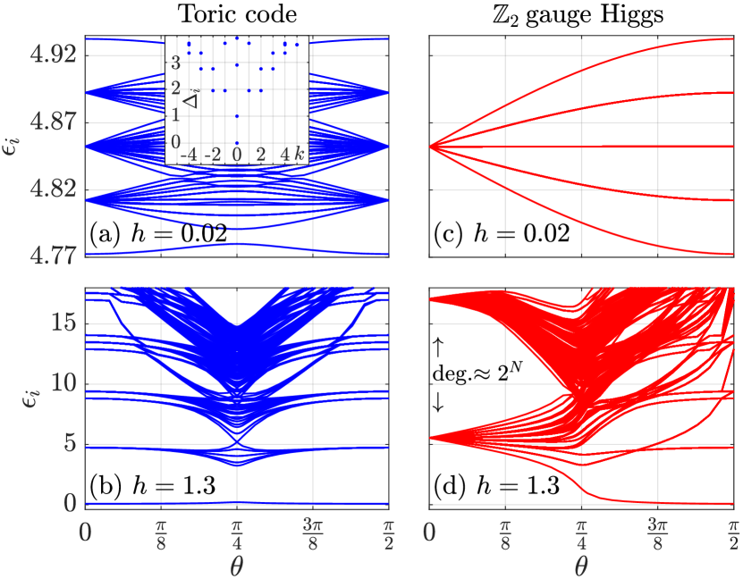
Figure 2: Entanglement spectra. Entanglement spectra $\{\epsilon_{i}\}$ ($\epsilon_{0}\geq\epsilon_{1}\geq\epsilon_{2}\geq\cdots$) for systems on an infinitely long cylinder with a finite circumference. Along $h=0.02$ [$1.3$], the boundary MPO has the physical and virtual bond dimensions $(D,\chi)=(2,10)$ [$(2,40)$]. (a) ES of the TC model along $h=0.02$ with $N=8$. Inset: Momentum resolved ES at $\theta=\pi/4$ with $N=10$, $k$ is the lattice momentum in units of $2\pi/N$ and $\Delta_{i}$ is shifted and rescaled ES $\{(\Delta_{i}=\epsilon_{i}-\epsilon_{0})/\epsilon_{1}\}$, which we compare with the scaling dimensions (0,1,2,$\cdots$) of the Ising CFT. (b) ES of the TC model along $h=1.3$ with $N=8$ in the trivial phase. (c) and (d) ES of the $\mathbb{Z}_{2}$ GH model ($N=8$) along $h=0.02$ in the deconfined and $h=1.3$ in the Higgs-confined phase.

Entanglement Hamiltonian and ES of the $\mathbb{Z}_{2}$ GH model. By applying the quantum channel $\mathscr{N}[\cdot]$ to the reduced density matrix of the TC model, we derive the effective entanglement Hamiltonian of the $\mathbb{Z}_{2}$ GH model $\tilde{H}_{E,\text{GH}}$, whose dominant part is a classical Ising chain, see supplement [23],

$$\tilde{H}_{E,\text{GH}}=\left[(N-1)\log 2-\frac{h_{x}}{2}\sum_{i=1}^{L}X_{i}X_{i+1}+O(h^{2})\right]P_{+}.$$ (7)

Comparing $\tilde{H}_{E,\text{TC}}$ and $\tilde{H}_{E,\text{GH}}$, the transverse field term $\sum_{i}Z_{i}$ is absent. This is because $Z_{i}$ in $\tilde{H}_{E,\text{TC}}$ corresponds to the term $\Tr_{L}\left(Z_{e\in\partial L}\ket{\text{TC}}\bra{\text{TC}}\right)$ in $\rho_{\text{TC}}$, which anti-commutes with $X_{e^{\prime}\in\partial R}$, where $e$ and $e^{\prime}$ are in the same plaquette. By mapping $\rho_{\text{TC}}$ to $\rho_{\text{GH}}$ using the quantum channel $\mathscr{N}[\cdot]$, we find that $\mathscr{N}[\Tr_{L}\left(Z_{e\in\partial L}\ket{\text{TC}}\bra{\text{TC}}\right)]=0$, according to the property (ii) of the quantum channel $\mathscr{N}[\cdot]$ and thus the term $\propto$$\sum_{i}Z_{i}$ disappears. Moreover, for $h\rightarrow\infty$ and $\theta\neq\pi/2$, we derive the effective entanglement Hamiltonian of the $\mathbb{Z}_{2}$ GH model [23],

$$\tilde{H}_{E,\text{GH}}=-\sum_{i=1}^{N}\text{arctanh}(\sin\theta)X_{i}+N\log[\cos(\theta)/2].$$ (8)

In contrast to the TC model, where $\tilde{H}_{E,\text{TC}}=0$ for all $\theta$, we find for the $\mathbb{Z}_{2}$ GH model that $\tilde{H}_{E,\text{GH}}=0$ only for $\theta=\pi/2$.

An efficient way to calculate the ES of the $\mathbb{Z}_{2}$ GH model is to apply the quantum channel $\mathscr{N}[\cdot]$ to extract the ES of the $\mathbb{Z}_{2}$ GH model directly from the boundary MPO of the TC model [23]; Figs. 2c and  2d. Comparing to Fig. 2a and b, we observe that the ES of the $\mathbb{Z}_{2}$ GH model are the same as those of the TC model only when $\theta=\pi/2$, where the matter field and gauge field are no longer entangled. Moreover, the ES of the $\mathbb{Z}_{2}$ GH model are no longer symmetric about $\pi/4$. This raises the question of why the modified duality transformation $U_{\text{GH}}$ of the $\mathbb{Z}_{2}$ GH model fails to enforce the ES to be symmetric about $\pi/4$. Considering the duality transformation $U_{E,\text{TC}}$ that is applied to $\rho_{\text{TC}}$, the duality transformation applied to $\rho_{\text{GH}}=\mathscr{N}[\rho_{\text{TC}}]$ is $\mathscr{U}_{E,\text{GH}}[\cdot]=\mathscr{N}[U_{E,\text{TC}}\mathscr{N}^{-1}[\cdot]U_{E,\text{TC}}^{\dagger}]$. As $\rho_{\text{GH}}$ satisfies property (iii) of the quantum channel $\mathscr{N}[\cdot]$, there exists $\mathscr{N}^{-1}[\cdot]$. For $\mathscr{U}_{E,\text{GH}}[\cdot]$ to still apply in the usual way, there should exist a unitary matrix $U_{E,\text{GH}}$, such that $\mathscr{U}_{E,\text{GH}}[\cdot]=U_{E,\text{GH}}\cdot U^{\dagger}_{E,\text{GH}}$. If such a $U_{E,\text{GH}}$ does not exist, $\mathscr{U}_{E,\text{GH}}$ applied to $\rho_{\text{GH}}$ will no longer be a unitary transformation and consequently the spectra of $\rho_{\text{GH}}(h_{x},h_{z})$ and $\rho_{\text{GH}}(h_{z},h_{x})$ will generically be different. So it is possible to have a non-symmetric ES even when the model has the duality symmetry.

Each level of the ES for the $\mathbb{Z}_{2}$ GH model has an extensive $2^{N-1}$-fold degeneracy in the deconfined phase along $h_{z}$ axis; Fig. 2c. By contrast, in the Higgs phase along $h_{z}$ axis, the degeneracy is enhanced to $2^{N}$ in the thermodynamic limit $(N\rightarrow\infty)$ due to charge condensation (for finite $N$ this degeneracy is weakly lifted to two branches and each has a degeneracy $2^{N-1}$); Fig. 2d. The extensive degeneracy on the $h_{z}$ axis arises from the interplay between the (open) Wilson loop and the gauge symmetry of $\rho_{\text{GH}}$, see proof in [23].

An interesting question is whether the bulk boundary correspondence holds, i.e., whether the findings made for the ES also apply to the energy spectrum of a system with open boundary conditions. In Ref. [13] a two-fold boundary degeneracy was found in the energy spectrum under specifically chosen boundary conditions, as well as a boundary phase transition separating the Higgs and confined phases. By contrast, both the entanglement Hamiltonian Eq. (8) and the ES in Fig. 2d do not exhibit such a phase transition. Since for quantum states of gauge theories, the entanglement Hamiltonian and the open boundary system can potentially have different symmetries, i.e., the open boundary systems do not necessarily have the local gauge symmetry $\{X_{e}|e\in\partial R\}$, they can exhibit different low-energy physics. Thus this is an example where the bulk-boundary correspondence fails.

Distillable entanglement entropy of the $\mathbb{Z}_{2}$ GH model.

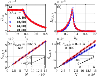
Figure 3: Rényi entanglement entropy of the $\mathbb{Z}_{2}$ GH model. (a) Total and (b) distillable $1/2$-Rényi entanglement entropy densities for a pure gauge theory ($h_{z}=0$) extrapolated to the thermodynamic limit. (c) Distillable Rényi entanglement entropy $S_{D,1/2}(\rho_{\text{GH}})$ at $(h,\theta)=(0.15,0.18\pi)$. Inset: Zoom in of the extrapolation yielding the topological correction $\gamma_{D}=\log(2)$. (d) $S_{D,1/2}(\rho_{\text{GH}})$ at $(h,\theta)=(0.26,\pi/2)$. Inset: No correction to the area law is detected.

The entanglement entropy $S$ in the toric code phase satisfies $S=\alpha N-\gamma$, where $\alpha$ is a non-universal constant and $\gamma=\log 2$ is the universal topological entanglement entropy (TEE) characterizing the $\mathbb{Z}_{2}$ topological order [3, 4, 30]. Since the isometry $V$ connecting the TC model and the $\mathbb{Z}_{2}$ GH model is a constant depth quantum circuit, which cannot change the $\mathbb{Z}_{2}$ topological order [31], the deconfined phase and the toric code phase have the same TEE.

Entanglement of gauge theories exhibits a richer structure because of the gauge constraints [14, 15]. Specifically, the reduced density matrix for the $\mathbb{Z}_{2}$ GH model is block diagonal [14] due to the gauge symmetry $[\rho_{\text{GH}},X_{e}]=0,\forall e\in R$,

$$\rho_{\text{GH}}=\bigoplus_{\boldsymbol{x}}p_{\boldsymbol{x}}\rho_{\text{GH},\boldsymbol{x}},\quad\rho_{\text{GH},\boldsymbol{x}}=\rho_{\text{GH}}P_{\boldsymbol{x}}/p_{\boldsymbol{x}},\quad p_{\boldsymbol{x}}=\Tr\left(P_{\boldsymbol{x}}\rho_{\text{GH}}\right),$$ (9)

where $P_{\boldsymbol{x}}=2^{-N}\prod_{e\in\partial R}(1+x_{e}X_{e})$ and $x_{e}=\pm 1$. Moreover, $\rho_{\text{GH},\boldsymbol{x}}$ is the reduced density matrix of a pure state $P_{\boldsymbol{x}}\ket{\Psi_{\text{GH}}}/\sqrt{p_{\boldsymbol{x}}}$, obtained by fixing gauge field in $\partial R$ by the measurement of $X$ operators; Fig. 1a. The probability of the measurement outcome $\ket{\boldsymbol{x}}$ is $p_{\boldsymbol{x}}$. In fact, the dominant classical parts (diagonal in the $X$ basis) of the entanglement Hamiltonians in Eqs. (7) and (8), as well as the ES in Figs. 2c and  2d, reflect the probability distributions $\{p_{\boldsymbol{x}}\}$. Hence the von Neumann entanglement entropy $S(\rho_{\text{GH}})=-\Tr(\rho_{\text{GH}}\log\rho_{\text{GH}})$ can be separated into two parts [32, 14]: $S(\rho_{\text{GH}})=-\sum_{\boldsymbol{x}}p_{\boldsymbol{x}}\log p_{\boldsymbol{x}}+\sum_{\boldsymbol{x}}p_{\boldsymbol{x}}S(\rho_{\text{GH},\boldsymbol{x}})$. The first part is the Shannon entropy of the probability distribution $\{p_{\boldsymbol{x}}\}$. The second part $\quad S_{D}(\rho_{\text{GH}})=\sum_{\boldsymbol{x}}p_{\boldsymbol{x}}S(\rho_{\text{GH},\boldsymbol{x}})$ is the distillable entanglement entropy , characterizing the entanglement that can be detected by gauge invariant local operator operations [14, 15, 32]. Such a decomposition of the entanglement can be applied to any quantum state with symmetry, e.g., symmetry protected topological states [34].

We now study how the distillable entanglement entropy $S_{D}$ depends on the subsystem size. In Ref. [15] it is conjectured that $S_{D}(\rho_{\text{GH}})=0$ when the $\mathbb{Z}_{2}$ GH model reduces to a pure gauge theory ($h_{z}=0$) and $S_{D}(\rho_{\text{GH}})=\alpha^{\prime}N-\log 2$, where $\alpha^{\prime}$ is a nonuniversal constant, in the deconfined phase with finite gauge-matter coupling ($h_{z}\neq 0$). We use tensor-network methods to check these conjectures. Since it is easier to compute the $n$-Rényi entanglement entropy $S_{n}(\rho)=(1-n)^{-1}\log\Tr\rho^{n}$ rather than the von Neumann entropy in tensor network methods, and Ref. [35] provides the Rényi generalization of the distillable entanglement entropy, we consider the distillable Rényi entanglement entropy with $n=1/2$: $S_{D,1/2}(\rho_{\text{GH}})=\log\sum_{\boldsymbol{x}}p_{\boldsymbol{x}}\left(\Tr\sqrt{\rho_{\text{GH},\boldsymbol{x}}}\right)^{2}$ [23]. Using the quantum channel, we find $\rho_{\text{GH},\boldsymbol{x}}=P_{\boldsymbol{x}}\mathscr{N}[\rho_{\text{TC}}]P_{\boldsymbol{x}}=\tilde{V}^{\dagger}_{\boldsymbol{x}}\rho_{\text{TC},\boldsymbol{x}}\tilde{V}^{\dagger}_{\boldsymbol{x}}$, where $\tilde{V}_{\boldsymbol{x}}$ is another isometric matrix and $\rho_{\text{TC},\boldsymbol{x}}=P_{\boldsymbol{x}}\rho_{\text{TC}}P_{\boldsymbol{x}}/p_{\boldsymbol{x}}$ (Notice that $[P_{\boldsymbol{x}},\rho_{\text{TC}}]\neq 0$ in general). Thus $S(\rho_{\text{GH},\boldsymbol{x}})=S(\rho_{\text{TC},\boldsymbol{x}})$ and $S_{D,1/2}$ of the $\mathbb{Z}_{2}$ GH model can be calculated from TC iPEPS efficiently for arbitrary circumference $N$ [23].

We compute the total and distillable Rényi entanglement entropy densities of the $\mathbb{Z}_{2}$ GH along $h_{x}$ axis; Fig. 3a and b. In contrast to the conjecture in Ref. [15], our numerical results indicate that the distillable entanglement entropy can be non-zero for the pure gauge theory with finite $h_{x}$. In addition to the area law, the distillable Rényi entanglement entropy in the deconfined phase with gauge-matter coupling ($h_{z}\neq 0$) has a correction $\gamma_{D}=\log 2$; Fig. 3c. This correction vanishes $\gamma_{D}=0$ for the pure gauge theory ($h_{z}=0$); Fig. 3d. For the pure gauge theory, $X$ measurements at $\partial R$ shown in Fig. 1a destroy the underlying long-range entanglement completely along the entanglement cut, because $P_{\boldsymbol{x}}$ commutes with the gauge fluctuations in Eq. (3), and only short-range entanglement can be retained. However, when $h_{z}\neq 0$, the gauge-matter coupling in Eq. (3), which does not commute with $P_{\boldsymbol{x}}$, prevents the $X$ measurements at $\partial R$ from destroying the long-range entanglement along the entanglement cut, giving rise to the distillable TEE $\gamma_{D}=\log 2$ (see [23] for additional details).

Discussion and outlook. The TC model and $\mathbb{Z}_{2}$ GH model are related by an isometric transformation. We show that the isometry acting on a subsystem acts as a quantum channel. As a consequence, we find that although the reduced density matrix of the TC is entailed with the electric-magnetic duality symmetry, this is not the case for the $\mathbb{Z}_{2}$ GH model. Our results demonstrate that combining quantum channels with tensor networks is useful for extracting entanglement properties of systems related by an isometric transformation. Similar considerations as discussed here, also hold for the deformed wavefunctions of the TC model and $\mathbb{Z}_{2}$ GH model [36, 37].

Our approach can be used to study the entanglement of any two wavefunctions transformed by a constant depth circuit, for example, to extract the entanglement of a non-trivial symmetry-protected (enriched) topological state from the trivial one [38, 39]. Our results can also be generalized to other Abelian lattice gauge theories of finite groups with matter fields. Moreover, it would be interesting to investigate the entanglement of non-Abelian gauge theories and topological phases with self-duality [40, 41], as well as gauge theories with continuous groups [42].

Acknowledgements. We especially thank Ari Turner for many useful discussions on this work and prior collaborations on entanglement transitions. We also thank R.-Z. Huang and Ruben Verresen for helpful comments. We acknowledge support from the Deutsche Forschungsgemeinschaft (DFG, German Research Foundation) under Germany’s Excellence Strategy–EXC–2111–390814868, TRR 360 – 492547816 and DFG grants No. KN1254/1-2, KN1254/2-1, the European Research Council (ERC) under the European Union’s Horizon 2020 research and innovation programme (grant agreement No. 851161 and No. 771537), as well as the Munich Quantum Valley, which is supported by the Bavarian state government with funds from the Hightech Agenda Bayern Plus.

Data availability – Data, data analysis, and simulation codes are available upon reasonable request on Zenodo [43].

Appendix A Quantum channel and its properties

In this section, we show how to derive the Kraus operators, prove $\mathscr{N}[\cdot]$ is a quantum channel, and show some useful properties of the quantum channel. At first, we derive the Kraus operators, which transform the density operator $\rho_{\text{TC}}$ to $\rho_{\text{GH}}$:

$$\rho_{\text{GH}} =\Tr_{L}\left(\ket{\Psi_{\text{GH}}}\bra{\Psi_{\text{GH}}}\right)=\Tr_{L}\left(V\ket{\Psi_{\text{TC}}}\bra{\Psi_{\text{TC}}}V^{\dagger}\right)$$

$$=\Tr_{L}\left[\left(\prod_{\langle e,v\rangle}\text{CX}_{v,e}\prod_{v}\ket{+}_{v}\right)\ket{\Psi_{\text{TC}}}\bra{\Psi_{\text{TC}}}\left(\prod_{v}\bra{+}_{v}\prod_{\langle v,e\rangle}\text{CX}_{v,e}\right)\right]$$

$$=\Tr_{L}\left[\left(\prod_{\langle v\in(\partial L\cup R),e\in R\rangle}\text{CX}_{v,e}\prod_{v\in\partial L\cup R}\ket{+}_{v}\right)\ket{\Psi_{\text{TC}}}\bra{\Psi_{\text{TC}}}\left(\prod_{v\in\partial L\cup R}\bra{+}_{v}\prod_{\langle v\in(\partial L\cup R),e\in R\rangle}\text{CX}_{v,e}\right)\right]$$

$$=\frac{1}{2^{N}}\sum_{\{z_{v}=\pm 1|v\in\partial L\}}\left(\prod_{\langle v\in\partial L,e\in\partial R\rangle}X_{e}^{\frac{1-z_{v}}{2}}\prod_{\langle v\in R,e\in R\rangle}\text{CX}_{v,e}\prod_{v\in R}\ket{+}_{v}\right)\rho_{\text{TC}}\left(\prod_{v\in R}\bra{+}_{v}\prod_{\langle v\in R,e\in(R)\rangle}\text{CX}_{v,e}\prod_{\langle v\in\partial L,e\in\partial R\rangle}X_{e}^{\frac{1-z_{v}}{2}}\right)$$

$$=\sum_{\boldsymbol{z}}K_{\boldsymbol{z}}\rho_{\text{TC}}K_{\boldsymbol{z}}^{\dagger}=\mathscr{N}[\rho_{\text{TC}}].$$ (10)

Therefore, we have the Kraus operators as shown in Eq. (5). Notice that the mapping $\mathscr{N}[\cdot]$ defined by the Kraus operators is completely positive. In order to prove that it is a quantum channel, we need to prove that trace-preserving condition: $\sum_{\boldsymbol{z}}K_{\boldsymbol{z}}^{\dagger}K_{\boldsymbol{z}}=\mathbbm{1}$. Because

$$\sum_{\boldsymbol{z}}{K_{\boldsymbol{z}}^{\dagger}K_{\boldsymbol{z}}}=\frac{1}{2^{N}}\prod_{v}\bra{+}_{v}\sum_{\{z_{v}=\pm 1|v\in\partial L\}}\left(\prod_{\langle v\in\partial L,e\in\partial R\rangle}X_{e}^{\frac{1-z_{v}}{2}}\prod_{\langle v\in R,e\in R\rangle}\text{CX}_{v,e}\prod_{\langle v\in R,e\in(R)\rangle}\text{CX}_{v,e}\prod_{\langle v\in\partial L,e\in\partial R\rangle}X_{e}^{\frac{1-z_{v}}{2}}\right)\ket{+}_{v}=\mathbbm{1},$$ (11)

the mapping $\mathscr{N}[\cdot]$ is indeed trace-preserving and is a quantum channel, as we expected since $V$ is an isometric matrix.

It is interesting to check if the quantum channel satisfies the unital condition: $\sum_{\boldsymbol{z}}K_{\boldsymbol{z}}K^{\dagger}_{\boldsymbol{z}}=\mathbbm{1}$. Because

$$\sum_{\boldsymbol{z}}K_{\boldsymbol{z}}K^{\dagger}_{\boldsymbol{z}}=\frac{1}{2^{N}}\sum_{\{z_{v}=\pm 1|v\in\partial L\}}\left(\prod_{\langle v\in\partial L,e\in\partial R\rangle}X_{e}^{\frac{1-z_{v}}{2}}\prod_{\langle v\in R,e\in R\rangle}\text{CX}_{v,e}\prod_{v\in R}\frac{1+X_{v}}{2}\prod_{\langle v\in R,e\in(R)\rangle}\text{CX}_{v,e}\prod_{\langle v\in\partial L,e\in\partial R\rangle}X_{e}^{\frac{1-z_{v}}{2}}\right)=\prod_{v\in R}\frac{1+X_{v}A_{v}}{2},$$ (12)

where we use the relation

$$\left(\prod_{\langle v,e\rangle}\text{CX}_{v,e}\right)\frac{1+X_{v}}{2}\left(\prod_{\langle v,e\rangle}\text{CX}_{v,e}\right)=\frac{1+X_{v}A_{v}}{2},\\$$ (13)

the quantum channel is not unital in general because it maps the identity matrix to a projector. However, we can restrict to the subspace of the total Hilbert space satisfying the gauge constraint, where the projector $(1+X_{v}A_{v})/2$ becomes an identity operator, such that the quantum channel $\mathscr{N}[\cdot]$ is unital in this subspace.

Moreover, we can also prove that the quantum channel $\mathscr{N}[\cdot]$ has a right inverse under some extra conditions, which means that $\exists\mathscr{N}^{-1}[\cdot]$ such that $\mathscr{N}[\mathscr{N}^{-1}[\rho_{\text{GH}}]]=\rho_{\text{GH}}$ for certain $\rho_{\text{GH}}$. Consider $\sum_{{\boldsymbol{z}}^{\prime},\boldsymbol{z}}K_{{\boldsymbol{z}}^{\prime}}K_{\boldsymbol{z}}^{\dagger}\rho_{\text{GH}}K_{\boldsymbol{z}}K_{\boldsymbol{z}^{\prime}}^{\dagger}$, because

$$K_{{\boldsymbol{z}}^{\prime}}K^{\dagger}_{\boldsymbol{z}}=\frac{1}{2^{N}}\left(\prod_{\langle v\in\partial L,e\in\partial R\rangle}X_{e}^{\frac{1-z^{\prime}_{v}}{2}}\prod_{\langle v\in R,e\in R\rangle}\text{CX}_{v,e}\prod_{v\in R}\frac{1+X_{v}}{2}\prod_{\langle v\in R,e\in(R)\rangle}\text{CX}_{v,e}\prod_{\langle v\in\partial L,e\in\partial R\rangle}X_{e}^{\frac{1-z_{v}}{2}}\right)=\frac{1}{2^{N}}\prod_{v\in R}\frac{1+X_{v}A_{v}}{2}\prod_{\langle v\in\partial L,e\in\partial R\rangle}X_{e}^{\frac{1-z^{\prime}_{v}z_{v}}{2}},$$ (14)

we have

$$\sum_{{\boldsymbol{z}}^{\prime},\boldsymbol{z}}K_{{\boldsymbol{z}}^{\prime}}K_{\boldsymbol{z}}^{\dagger}\rho_{\text{GH}}K_{\boldsymbol{z}}K_{{\boldsymbol{z}}^{\prime}}^{\dagger}=\frac{1}{4^{N}}\prod_{v\in R}\frac{1+X_{v}A_{v}}{2}\sum_{\boldsymbol{z},\boldsymbol{z}^{\prime}}\prod_{\langle v\in\partial L,e\in\partial R\rangle}X_{e}^{\frac{1-z^{\prime}_{v}z_{v}}{2}}\rho_{\text{GH}}\prod_{\langle v\in\partial L,e\in\partial R\rangle}X_{e}^{\frac{1-z^{\prime}_{v}z_{v}}{2}}\prod_{v\in R}\frac{1+X_{v}A_{v}}{2}=\rho_{\text{GH}}.$$ (15)

where the last identity is valid if

$$X_{e}\rho_{\text{GH}}X_{e}=\rho_{\text{GH}},\forall e\in\partial R,\quad\rho_{\text{GH}}X_{v}A_{v}=X_{v}A_{v}\rho_{\text{GH}}=\rho_{\text{GH}},\forall v\in R.$$ (16)

Hence, the quantum channel $\mathscr{N}[\cdot]$ has a right inverse $\mathscr{N}^{-1}[\cdot]=\sum_{\boldsymbol{z}}K_{\boldsymbol{z}}\cdot K_{\boldsymbol{z}}^{\dagger}$ if the conditions in Eq. (16) are satisfied. And we know the reduced density matrix $\rho_{\text{GH}}$ of any gauge invariant state $\ket{\Psi_{\text{GH}}}$ ($X_{v}A_{v}\ket{\Psi_{\text{GH}}}=\ket{\Psi_{\text{GH}}},\forall v$) satisfies the conditions in Eq. (16), and $\mathscr{N}^{-1}[\cdot]$ is a quantum channel if we only consider the reduced density matrices of gauge invariant quantum states.

Let us also consider the relevant symmetry and the null space of the channel operator. It is not difficult to check that the quantum channel satisfies:

$$\mathscr{N}[\cdot]=X_{e}\mathscr{N}[\cdot]X_{e}=\mathscr{N}[X_{e}\cdot X_{e}],\quad\forall e\in\partial R.$$ (17)

Consider an operator $O$ living in the input Hilbert space of the quantum channel, if $\exists e\in\partial R$, such that $\{X_{e},O\}=0$, then $\mathscr{N}[O]=\mathscr{N}[X_{e}OX_{e}]=-\mathscr{N}[O]$, and $\mathscr{N}[O]=0$. It means that any operator that anti-commutes with the gauge symmetry is in the null space of the quantum channel.

Next, let’s talk about how to calculate the distillable entanglement entropy of a state in the Hilbert space of $\mathbb{Z}_{2}$ GH model from a corresponding state in the Hilbert space of the TC model. According to the definition of the distillable entanglement entropy, we consider a state $P_{\boldsymbol{x}}\ket{\Psi_{\text{GH}}}=\ket{\boldsymbol{x}}\bra{\boldsymbol{x}}\ket{\Psi_{\text{GH}}}$ obtained by fixing physical degrees of freedom in $\partial R$ to $\ket{\boldsymbol{x}}=\prod_{e\in\partial R}|x_{e}\rangle$:

$$\Tr_{L}P_{\boldsymbol{x}}\ket{\Psi_{\text{GH}}}\bra{\Psi_{\text{GH}}}=P_{\boldsymbol{x}}\rho_{\text{GH}}=P_{\boldsymbol{x}}\rho_{\text{GH}}P_{\boldsymbol{x}}=P_{\boldsymbol{x}}\mathscr{N}(\rho_{\text{TC}})P_{\boldsymbol{x}}$$

$$=\frac{1}{2^{N}}\left[\ket{\boldsymbol{x}}\sum_{\{z_{v}=\pm 1|v\in\partial L\}}\left(\prod_{\langle v\in\partial L,e\in\partial R\rangle}x_{e}^{\frac{1-z_{v}}{2}}\bra{\boldsymbol{x}}\prod_{\langle v\in R,e^{\prime}\in R\rangle}\text{CX}_{v,e^{\prime}}\prod_{v\in R}\ket{+}_{v}\right)\rho_{\text{TC}}\left(\prod_{v\in R}\bra{+}_{v}\prod_{\langle v\in R,e^{\prime}\in(R)\rangle}\text{CX}_{v,e^{\prime}}\ket{\boldsymbol{x}}\prod_{\langle v\in\partial L,e\in\partial R\rangle}x_{e}^{\frac{1-z_{v}}{2}}\right)\bra{\boldsymbol{x}}\right]$$

$$=\left[\ket{\boldsymbol{x}}\left(\prod_{\langle v\in R,e\in\partial R\rangle}x_{e}^{\frac{1-Z_{v}}{2}}\prod_{\langle v\in R,e^{\prime}\in(R-\partial R)\rangle}\text{CX}_{v,e^{\prime}}\prod_{v\in R}\ket{+}_{v}\right)\bra{\boldsymbol{x}}\rho_{\text{TC}}\ket{\boldsymbol{x}}\left(\prod_{v\in R}\bra{+}_{v}\prod_{\langle v\in R,e^{\prime}\in(R-\partial R)\rangle}\text{CX}_{v,e^{\prime}}\prod_{\langle v\in R,e\in\partial R\rangle}x_{e}^{\frac{1-Z_{v}}{2}}\right)\bra{\boldsymbol{x}}\right]$$

$$=\tilde{V}_{\boldsymbol{x}}P_{\boldsymbol{x}}\rho_{\text{TC}}P_{\boldsymbol{x}}\tilde{V}^{\dagger}_{\boldsymbol{x}}=\tilde{V}_{\boldsymbol{x}}\Tr_{L}\left(P_{\boldsymbol{x}}\ket{\Psi_{\text{TC}}}\bra{\Psi_{\text{TC}}}P_{\boldsymbol{x}}\right)\tilde{V}^{\dagger}_{\boldsymbol{x}},$$ (18)

where $\tilde{V}_{\boldsymbol{x}}=\prod_{\langle v\in R,e\in\partial R\rangle}x_{e}^{\frac{1-Z_{v}}{2}}\prod_{\langle v\in R,e^{\prime}\in(R-\partial R)\rangle}\text{CX}_{v,e^{\prime}}\prod_{v\in R}\ket{+}_{v}$ satisfying $\tilde{V}^{\dagger}_{\boldsymbol{x}}\tilde{V}_{\boldsymbol{x}}=\mathbbm{1}$ is an isometric operator which applies on physical degrees of freedom in $(R-\partial R)$. Eq. (A) tells us

$$\rho_{\text{GH},\boldsymbol{x}}=\tilde{V}_{\boldsymbol{x}}\rho_{\text{TC},\boldsymbol{x}}\tilde{V}^{\dagger}_{\boldsymbol{x}},\quad p_{\boldsymbol{x}}=\bra{\Psi_{\text{TC}}}P_{\boldsymbol{x}}\ket{\Psi_{\text{TC}}}=\bra{\Psi_{\text{GH}}}P_{\boldsymbol{x}}\ket{\Psi_{\text{GH}}},$$ (19)

where

$$\rho_{\text{TC},\boldsymbol{x}}=\Tr_{L}\left(P_{\boldsymbol{x}}\ket{\Psi_{\text{TC}}}\bra{\Psi_{\text{TC}}}P_{\boldsymbol{x}}\right)/p_{\boldsymbol{x}},\quad\quad\rho_{\text{GH},\boldsymbol{x}}=\Tr_{L}\left(P_{\boldsymbol{x}}\ket{\Psi_{\text{GH}}}\bra{\Psi_{\text{GH}}}P_{\boldsymbol{x}}\right)/p_{\boldsymbol{x}}.$$

So we have $S(\rho_{\text{GH},\boldsymbol{x}})=S(\rho_{\text{TC},\boldsymbol{x}})$ according to Eq. (19), and we can calculate the distillable entanglement entropy of a state living in the Hilbert space of the $\mathbb{Z}_{2}$ GH model by fixing degrees of freedom of a corresponding TC state in $\partial R$: $P_{\boldsymbol{x}}\ket{\Psi_{\text{TC}}}$.

Finally, let us prove $\rho_{\text{GH}}$ has an extensive $2^{N-1}$ fold degeneracy observed in Fig. 2 (c) and (d) at $\theta=0$, where $\ket{\Psi_{\text{GH}}}$ has the symmetry of Wilson loops: $W^{Z}_{C}\ket{\Psi_{\text{GH}}}=\ket{\Psi_{\text{GH}}},\forall C$, and $W^{Z}_{C}=\prod_{e\in C}Z_{e}$ is a Wilson loop operator and $C$ is a closed loop along the lattice. The reduced density matrix has the symmetry of open Wilson loops: $[W^{Z}_{C/2},\rho_{\text{GH}}]=0,\forall C/2$, where $C/2$ is an open loop whose two ends $e,e^{\prime}\in\partial R$. Because

$$W^{Z}_{C/2}P_{\boldsymbol{x}}\rho_{\text{GH}}W^{Z}_{C/2}=P_{\boldsymbol{x}^{\prime}}W^{Z}_{C/2}\rho_{\text{GH}}W^{Z}_{C/2}=P_{\boldsymbol{x}^{\prime}}\rho_{\text{GH}},$$ (20)

where $|\boldsymbol{x}^{\prime}\rangle=Z_{e\in\partial R}Z_{e^{\prime}\in\partial R}\ket{\boldsymbol{x}}$. From Eqs. (9) and  (20), it can be found that $p_{\boldsymbol{x}}=p_{\boldsymbol{x}^{\prime}}$ and $\rho_{\boldsymbol{x}}=W_{C/2}^{Z}\rho_{\boldsymbol{x}^{\prime}}W_{C/2}^{Z}$. Therefore $\rho_{\boldsymbol{x}}$ and $\rho_{\boldsymbol{x}^{\prime}}$ have the same spectrum. Since $[W_{C/2}^{Z}.\prod_{e\in\partial R}X_{e}]=0$, $\ket{\boldsymbol{x}}$ and $\ket{\boldsymbol{x}^{\prime}}$ have the same parity. Therefore the spectra of the blocks with the same parity are identical, and the ES of $\rho_{\text{GH}}$ has $2^{N-1}$-fold degenerate. Notice that the gauge symmetry $\{X_{e}|e\in\partial R\}$ is from the local gauge constraint crossing the entanglement cut and tracing the $L$ part, see Fig. 1a, the system with an open boundary does not necessary have this symmetry and the extensive degeneracy in low energy. Moreover, if we choose $\ket{\Psi_{\text{GH}}}$ as an eigenstate of $\prod_{e\in\partial R}X_{e}$, then $\rho_{\text{GH}}$ only contains blocks with even or odd parity, and we can say that $\rho_{\text{GH}}$ satisfies the so-called entanglement equaipartition [44].

Appendix B Effective entanglement Hamiltonians of the TC model from perturbation theory

In this section, we derive the entanglement Hamiltonians of all MES of the toric code by combining the tensor networks and perturbation theory. Before deriving the entanglement Hamiltonian, we define some conventions of the tensors:

$$\vbox{\hbox{ \includegraphics{delta_tensor.pdf}}}=\delta_{i_{1},i_{2}}\delta_{i_{2},i_{3}}\delta_{i_{3},i_{4}}\cdots\delta_{i_{n-1},i_{n}},\vbox{\hbox{ \includegraphics{Gauss_law_tensor.pdf}}}=\delta_{(i_{1}+i_{2}+\cdots i_{n})\text{mod}2,0},\vbox{\hbox{ \includegraphics{crossing.pdf}}}=\delta_{i_{1},i_{2}}\delta_{i_{3},i_{4}}.$$ (21)

The entries of the black dot tensor are 1 if all legs are equal. The entries of the black open circle tensor are $1$ if the total parity of all legs is even; otherwise, the entries are $0$. If two straight lines cross, it represents a tensor product of two identity matrices. With these definitions, we can define the single-line PEPS for four MES of the TC model at $h=0$ [45], as shown in Figs. 4a and  4b.

The reduced density $\rho$ matrix of an injective PEPS $\ket{\Psi}$ contains a large null space, an isometric transformation $\mathcal{V}$ can be found to transform $\rho$ to the low entanglement energy subspace (spanned by eigenvectors of $\rho$ with non-zero eigenvalues). The transformed reduced density matrix can be expressed in terms of left and right fixed points $\sigma_{L}$ and $\sigma_{R}$ of the PEPS transfer matrix [26]:

$$\mathcal{V}\rho\mathcal{V}^{\dagger}=\mathcal{V}\left(\Tr_{L}\ket{\Psi}\bra{\Psi}\right)\mathcal{V}^{\dagger}\propto\sqrt{\sigma_{R}^{\text{T}}}\sigma_{L}\sqrt{\sigma_{R}^{\text{T}}},$$ (22)

where the isometry $\mathcal{V}$ satisfies $\mathcal{V}\mathcal{V}^{\dagger}=\mathbbm{1}$ and $\mathcal{V}^{\dagger}\mathcal{V}$ is a projector onto the low entanglement energy subspace, and $[\mathcal{V}^{\dagger}\mathcal{V},\rho]=0$.

Following Ref. [46], we know that the transfer matrix of the toric code PEPS at $h=0$ can be expressed as $\mathbb{T}=(\mathbbm{1}_{2}^{\otimes N}\otimes\mathbbm{1}_{2}^{\otimes N}+Z^{\otimes N}\otimes Z^{\otimes N})$. Because the PEPS of the toric code model at $h=0$ is $\mathbb{Z}_{2}$ injective, the left and right fixed points of the transfer matrix are equal and two-fold degenerate: $\sigma_{L}=\sigma_{R}=\mathbbm{1}_{2}^{\otimes N}$ or $Z^{\otimes N}$. Because the ground states of the TC model are four-fold degenerate, there are four reduced density matrices $\rho_{\text{TC}}^{\boldsymbol{\alpha},(0)},\boldsymbol{\alpha}=\boldsymbol{1},\boldsymbol{e},\boldsymbol{m}$ or $\boldsymbol{f}$ at $h=0$, which can be constructed from the superposition of the degenerate transfer matrix fixed points [46]:

$$\mathcal{V}^{\boldsymbol{1}}_{\text{TC}}\rho^{\boldsymbol{1},(0)}_{\text{TC}}\mathcal{V}^{\boldsymbol{1}\dagger}_{\text{TC}}=\mathcal{V}^{\boldsymbol{e}}_{\text{TC}}\rho^{\boldsymbol{e},(0)}_{\text{TC}}\mathcal{V}^{\boldsymbol{e}\dagger}_{\text{TC}}=\frac{1}{2^{N}}(\mathbbm{1}_{2}^{\otimes N}+Z^{\otimes N})=\frac{1}{2^{N-1}}P_{+},\quad\mathcal{V}^{\boldsymbol{m}}_{\text{TC}}\rho^{\boldsymbol{m},(0)}_{\text{TC}}\mathcal{V}^{\boldsymbol{m}\dagger}_{\text{TC}}=\mathcal{V}^{\boldsymbol{f}}_{\text{TC}}\rho^{\boldsymbol{f},(0)}_{\text{TC}}\mathcal{V}^{\boldsymbol{f}\dagger}_{\text{TC}}=\frac{1}{2^{N}}(\mathbbm{1}_{2}^{\otimes N}-Z^{\otimes N})=\frac{1}{2^{N-1}}P_{-},$$ (23)

where $\mathcal{V}_{\text{TC}}^{\boldsymbol{\alpha}}$ defined in Figs. 4c and  4d are nothing but half of the PEPS. These operators satisfy $\mathcal{V}^{\boldsymbol{\alpha}}_{\text{TC}}\mathcal{V}^{\boldsymbol{\alpha}\dagger}_{\text{TC}}=P_{\pm}=(\mathbbm{1}^{\otimes N}\pm Z^{\otimes N})/2$, which is equivalent to an identity matrix in the even or odd virtual subspace. And $\mathcal{V}^{\boldsymbol{\alpha}\dagger}_{\text{TC}}\mathcal{V}^{\boldsymbol{\alpha}}_{\text{TC}}$ is a projector from the 2D physical space to the 1D even or odd virtual subspace. So, these operators can still be viewed as isometries when restricted to low entanglement energy subspace with even or odd parity.

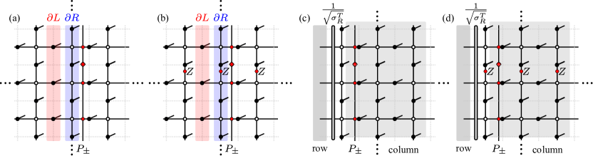
Figure 4: The iPEPS and isometries transforming the reduced density matrices to the low entanglement energy subspace. (a) The iPEPS representation of the MES $\ket{\text{TC}_{\boldsymbol{1}}}$ (when taking $P_{+}$) or $\ket{\text{TC}_{\boldsymbol{m}}}$ (when taking $P_{-}$) at $h=0$, the gray dotted lines are the lattice, the red diamond is $\mathbbm{1}_{2}$ for $P_{+}$ and $Z$ for $P_{-}$. The red cross tensor is defined as $\vbox{\hbox{ \includegraphics[width=14.22636pt]{zero_zero.pdf}}}=\mathbbm{1},\vbox{\hbox{ \includegraphics[width=14.22636pt]{one_one.pdf}}}=Z$. (b) The iPEPS of the MES $\ket{\text{TC}_{\boldsymbol{e}}}$ (when taking $P_{+}$) or $\ket{\text{TC}_{\boldsymbol{f}}}$ (when taking $P_{-}$). (c) The tensor network representation of the isometry $\mathcal{V}_{\boldsymbol{1}}$ (when taking $P_{+}$) or $\mathcal{V}_{\boldsymbol{m}}$ (when taking $P_{-}$), which is a tensor network whose up, right, and down parts are infinite, the dangling virtual legs on the left side consist of the row index of the isometry, and the physical legs on the right part of the system consist of the column index of the isometry. At $h=0$, we can simply take $\sigma_{R}=\mathbbm{1}$. (d) The isometry for $\mathcal{V}^{\boldsymbol{e}}_{\text{TC}}$ (when taking $P_{+}$) or $\mathcal{V}^{\boldsymbol{f}}_{\text{TC}}$ (when taking $P_{-}$).

Next, Let us consider the first-order perturbed wavefunction:

$$\ket{\Psi^{\boldsymbol{\alpha}}_{\text{TC}}}=\left[1+\frac{h_{x}}{4}\sum_{e}X_{e}+\frac{h_{z}}{4}\sum_{e}Z_{e}+O(h^{2})\right]\ket{\text{TC}_{\boldsymbol{\alpha}}},$$ (24)

where $\ket{\text{TC}_{\boldsymbol{\alpha}}}$ is a ground state at $h_{x}=h_{z}=0$ in terms of MES, see Figs. 4a and b. The reduced density matrix can be written as

$$\rho^{\boldsymbol{\alpha}}_{\text{TC}}=\Tr_{L}\ket{\Psi_{\text{TC}}^{\boldsymbol{\alpha}}}\bra{\Psi_{\text{TC}}^{\boldsymbol{\alpha}}}=\rho^{\boldsymbol{\alpha},(0)}_{\text{TC}}+\rho^{\boldsymbol{\alpha},(1)}_{\text{TC}}+O(h^{2}),$$ (25)

where

$$\rho^{\boldsymbol{\alpha},(0)}_{\text{TC}}=\Tr_{L}\ket{\text{TC}_{\boldsymbol{\alpha}}}\bra{\text{TC}_{\boldsymbol{\alpha}}},\quad\quad\rho^{\boldsymbol{\alpha},(1)}_{\text{TC}}=\frac{h_{x}}{4}\Tr_{L}\sum_{e\in E}\left(X_{e}\ket{\text{TC}_{\boldsymbol{\alpha}}}\bra{\text{TC}_{\boldsymbol{\alpha}}}+\text{h.c.}\right)+\frac{h_{z}}{4}\Tr_{L}\sum_{e\in E}\left(Z_{e}\ket{\text{TC}_{\boldsymbol{\alpha}}}\bra{\text{TC}_{\boldsymbol{\alpha}}}+\text{h.c.}\right).$$ (26)

Here, we also need an isometry to project onto the low-entanglement energy subspace. The previous isometry $\mathcal{V}^{\boldsymbol{\alpha}\dagger}_{\text{TC}}$ cannot do this exactly because $\mathcal{V}^{\boldsymbol{\alpha},\dagger}_{\text{TC}}\mathcal{V}^{\boldsymbol{\alpha}}_{\text{TC}}$ and $\rho^{\boldsymbol{\alpha}}_{\text{TC}}$ are only approximately commute. However, from the Schrieffer–Wolff transformation [47], we know that the error of using $\mathcal{V}^{\boldsymbol{\alpha}\dagger}_{\text{TC}}$ as an approximate isometry is $O(h^{2})$, so we have:

$$\mathcal{V}^{\boldsymbol{\alpha}}_{\text{TC}}\rho^{\boldsymbol{\alpha}}_{\text{TC}}\mathcal{V}^{\boldsymbol{\alpha}\dagger}_{\text{TC}}= \mathcal{V}^{\boldsymbol{\alpha}}_{\text{TC}}\left[\Tr_{L}\ket{\text{TC}_{\boldsymbol{\alpha}}}\bra{\text{TC}_{\boldsymbol{\alpha}}}+\frac{h_{x}}{4}\Tr_{L}\sum_{e\in\partial R}\left(X_{e}\ket{\text{TC}_{\boldsymbol{\alpha}}}\bra{\text{TC}_{\boldsymbol{\alpha}}}+\text{h.c.}\right)+\frac{h_{z}}{4}\sum_{e\in\partial L}\left(\Tr_{L}Z_{e}\ket{\text{TC}_{\boldsymbol{\alpha}}}\bra{\text{TC}_{\boldsymbol{\alpha}}}+\text{h.c.}\right)\right]\mathcal{V}^{\boldsymbol{\alpha}\dagger}_{\text{TC}}+O(h^{2}),$$ (27)

Notice that in the last two terms, we only sum over edges in $\partial L$ or $\partial R$ because other terms do not contribute to the zeroth and the first orders. For example, $\mathcal{V}^{\boldsymbol{\alpha}}_{\text{TC}}\Tr_{L}\left(X_{e}\ket{\text{TC}_{\boldsymbol{\alpha}}}\bra{\text{TC}_{\boldsymbol{\alpha}}}\right)\mathcal{V}^{\boldsymbol{\alpha}\dagger}_{\text{TC}}=0,\forall e\in(E-\partial R)$, because $\mathcal{V}^{\boldsymbol{\alpha}}_{\text{TC}}B_{p}=\mathcal{V}^{\boldsymbol{\alpha}}_{\text{TC}},B_{p}\ket{\text{TC}_{\boldsymbol{\alpha}}}=\ket{\text{TC}_{\boldsymbol{\alpha}}}$ and $\{B_{p},X_{e}\}=0,e\in p$, where $E$ is a set of all edges. For the same reason, $\mathcal{V}^{\boldsymbol{\alpha}}_{\text{TC}}\Tr_{L}\left(Z_{e}\ket{\text{TC}_{\boldsymbol{\alpha}}}\bra{\text{TC}_{\boldsymbol{\alpha}}}\right)\mathcal{V}^{\dagger}_{\boldsymbol{\alpha}}=0,\forall e\in(E-\partial L)$.

Let us consider the non-zero contributions. For a $Z_{e}\in\partial L$, it is convenient to transform it to the $R$ part using the relation $B_{p}\ket{\text{TC}_{\boldsymbol{\alpha}}}=\ket{\text{TC}_{\boldsymbol{\alpha}}}$:

$$\vbox{\hbox{ \includegraphics{Z_from_L2R.pdf}}}.$$ (28)

Then we can use the isometries shown on Figs. 4c and d to transform above three $Z$ operators as well as a $X_{e},e\in\partial R$ to the effective low entanglement energy space (virtual level of the single line tensor networks):

$$\vbox{\hbox{ \includegraphics{Z_physical_2_virtual.pdf}}}\quad,\quad\quad\vbox{\hbox{ \includegraphics{X_physical_2_virtual.pdf}}}\quad.$$ (29)

Then, the terms of the effective entanglement Hamiltonians can be derived from the above relations:

$$\mathcal{V}^{\boldsymbol{1}}_{\text{TC}}\Tr_{L}\left(X_{e}\ket{\text{TC}_{\boldsymbol{1}}}\bra{\text{TC}_{\boldsymbol{1}}}\right)\mathcal{V}^{\boldsymbol{1}\dagger}_{\text{TC}} =X_{i}X_{i+1}\mathcal{V}^{\boldsymbol{1}}_{\text{TC}}\Tr_{L}\left(\ket{\text{TC}_{\boldsymbol{1}}}\bra{\text{TC}_{\boldsymbol{1}}}\right)\mathcal{V}^{\boldsymbol{1}\dagger}_{\text{TC}}=X_{i}X_{i+1}P_{+}/2^{N-1},$$

$$\mathcal{V}^{\boldsymbol{m}}_{\text{TC}}\Tr_{L}\left(X_{e}\ket{\text{TC}_{\boldsymbol{m}}}\bra{\text{TC}_{\boldsymbol{m}}}\right)\mathcal{V}^{\boldsymbol{m}\dagger}_{\text{TC}} =X_{i}X_{i+1}\mathcal{V}^{\boldsymbol{m}}_{\text{TC}}\Tr_{L}\left(\ket{\text{TC}_{\boldsymbol{m}}}\bra{\text{TC}_{\boldsymbol{m}}}\right)\mathcal{V}^{\boldsymbol{m}\dagger}_{\text{TC}}=X_{i}X_{i+1}P_{-}/2^{N-1},$$

$$\mathcal{V}^{\boldsymbol{e}}_{\text{TC}}\Tr_{L}\left(X_{e}\ket{\text{TC}_{\boldsymbol{e}}}\bra{\text{TC}_{\boldsymbol{e}}}\right)\mathcal{V}^{\boldsymbol{e}\dagger}_{\text{TC}} =(-1)^{\delta_{N,i}}X_{i}X_{i+1}\mathcal{V}^{\boldsymbol{e}}_{\text{TC}}\Tr_{L}\left(\ket{\text{TC}_{\boldsymbol{e}}}\bra{\text{TC}_{\boldsymbol{1}}}\right)\mathcal{V}^{\boldsymbol{e}\dagger}_{\text{TC}}=(-1)^{\delta_{N,i}}X_{i}X_{i+1}P_{+}/2^{N-1},$$

$$\mathcal{V}^{\boldsymbol{f}}_{\text{TC}}\Tr_{L}\left(X_{e}\ket{\text{TC}_{\boldsymbol{f}}}\bra{\text{TC}_{\boldsymbol{f}}}\right)\mathcal{V}^{\boldsymbol{f}\dagger}_{\text{TC}} =(-1)^{\delta_{N,i}}X_{i}X_{i+1}\mathcal{V}^{\boldsymbol{f}}_{\text{TC}}\Tr_{L}\left(\ket{\text{TC}_{\boldsymbol{f}}}\bra{\text{TC}_{\boldsymbol{f}}}\right)\mathcal{V}^{\boldsymbol{f}\dagger}_{\text{TC}}=(-1)^{\delta_{N,i}}X_{i}X_{i+1}P_{-}/2^{N-1},$$

$$\mathcal{V}^{\boldsymbol{\alpha}}_{\text{TC}}\Tr_{L}\left(Z_{e}\ket{\text{TC}_{\boldsymbol{\alpha}}}\bra{\text{TC}_{\boldsymbol{\alpha}}}\right)\mathcal{V}^{\boldsymbol{\alpha}\dagger}_{\text{TC}} =Z_{i}\mathcal{V}^{\boldsymbol{\alpha}}_{\text{TC}}\Tr_{L}\left(\ket{\text{TC}_{\boldsymbol{\alpha}}}\bra{\text{TC}_{\boldsymbol{\alpha}}}\right)\mathcal{V}^{\boldsymbol{\alpha}\dagger}_{\text{TC}}=Z_{i}P_{\pm}/2^{N-1}.$$ (30)

Notice that the horizontal virtual $Z$ string shown in Fig. 4d introduces a minus sign when transforming a $X_{e},e\in\partial R$ to the effective low entanglement space. Therefore, the reduced density matrices in the low entanglement energy space can be expressed as

$$\mathcal{V}_{\text{TC}}^{\boldsymbol{1}}\rho^{\boldsymbol{1}}_{\text{TC}}\mathcal{V}_{\text{TC}}^{\boldsymbol{1}\dagger} =\frac{P_{+}}{2^{N-1}}\left(1+\frac{h_{x}}{2}\sum_{i=1}^{N}X_{i}X_{i+1}+\frac{h_{z}}{2}\sum_{i=1}^{N}Z_{i}+O(h^{2})\right),$$

$$\mathcal{V}_{\text{TC}}^{\boldsymbol{m}}\rho^{\boldsymbol{m}}_{\text{TC}}\mathcal{V}_{\text{TC}}^{\boldsymbol{m}\dagger} =\frac{P_{-}}{2^{N-1}}\left(1+\frac{h_{x}}{2}\sum_{i=1}^{N}X_{i}X_{i+1}+\frac{h_{z}}{2}\sum_{i=1}^{N}Z_{i}+O(h^{2})\right),$$

$$\mathcal{V}_{\text{TC}}^{\boldsymbol{e}}\rho^{\boldsymbol{e}}_{\text{TC}}\mathcal{V}_{\text{TC}}^{\boldsymbol{e}\dagger} =\frac{P_{+}}{2^{N-1}}\left(1+\frac{h_{x}}{2}\sum_{i=1}^{N}(-1)^{\delta_{N,i}}X_{i}X_{i+1}+\frac{h_{z}}{2}\sum_{i}Z_{i}+O(h^{2})\right),$$

$$\mathcal{V}_{\text{TC}}^{\boldsymbol{f}}\rho^{\boldsymbol{f}}_{\text{TC}}\mathcal{V}_{\text{TC}}^{\boldsymbol{f}\dagger} =\frac{P_{-}}{2^{N-1}}\left(1+\frac{h_{x}}{2}\sum_{i=1}^{N}(-1)^{\delta_{N,i}}X_{i}X_{i+1}+\frac{h_{z}}{2}\sum_{i=1}^{N}Z_{i}+O(h^{2})\right).$$ (31)

The effective entanglement Hamiltonian in each topological sector is $\tilde{H}^{\boldsymbol{\alpha}}_{E}=-\log(\mathcal{V}_{\text{TC}}^{\boldsymbol{\alpha}}\rho^{\boldsymbol{\alpha}}_{\text{TC}}\mathcal{V}_{\text{TC}}^{\boldsymbol{\alpha}\dagger})$. In the even or odd virtual subspace, the projectors $P_{\pm}$ becomes an identity matrix, and we can use the relation $\log(1+x)=x+O(x^{2})$ to derive the entanglement Hamiltonians:

$$\tilde{H}_{E,\text{TC}}^{\boldsymbol{1}}= \left[C-\sum_{i=1}^{N}\left(\frac{h_{z}}{2}Z_{i}+\frac{h_{x}}{2}X_{i}X_{i+1}\right)+O(h^{2})\right]P_{+},\quad\quad\tilde{H}_{E,\text{TC}}^{\boldsymbol{e}}=\left[C-\sum_{i=1}^{N}\left(\frac{h_{z}}{2}Z_{i}+(-1)^{\delta_{i,N}}\frac{h_{x}}{2}X_{i}X_{i+1}\right)+O(h^{2})\right]P_{+},$$

$$\tilde{H}_{E,\text{TC}}^{\boldsymbol{m}}= \left[C-\sum_{i=1}^{N}\left(\frac{h_{z}}{2}Z_{i}+\frac{h_{x}}{2}X_{i}X_{i+1}\right)+O(h^{2})\right]P_{-},\quad\quad\tilde{H}_{E,\text{TC}}^{\boldsymbol{f}}=\left[C-\sum_{i=1}^{N}\left(\frac{h_{z}}{2}Z_{i}+(-1)^{\delta_{i,N}}\frac{h_{x}}{2}X_{i}X_{i+1}\right)+O(h^{2})\right]P_{-},$$

where $C=(N-1)\text{log}2$. The method we use for deriving the entanglement Hamiltonian is similar to that shown in Ref. [48]. Moreover, we notice that the entanglement cut in Ref. [12] has a $\pi/4$ angle with the lattice of the TC model, and the resulting entanglement Hamiltonian is still approximately the Ising model. The difference is that the coefficients of the Ising model in Ref. [12] are proportional to $h^{2}_{x}$ and $h_{z}^{2}$, not $h_{x}$ and $h_{z}$. Furthermore, if we add the perturbations $\sum_{(e,e^{\prime})\in p}X_{e}X_{e^{\prime}}$ and $\sum_{(e,e^{\prime})\in v}Z_{e}Z_{e^{\prime}}$ to the Hamiltonian of the TC model, where $(e,e^{\prime})\in p$ [$(e,e^{\prime})\in v$] means a pair of edges in the same plaquette [vertex], they will results in the terms $\sum_{i}X_{i}X_{i+2}$ and $\sum_{i}Z_{i}Z_{i+1}$ in the low entanglement subspace, and the entanglement Hamiltonian will be described by the anisotropic next-nearest-neighboring Ising model.

Appendix C Effective entanglement Hamiltonians of the $\mathbb{Z}_{2}$ GH model from the quantum channel

In this section, we derive the entanglement Hamiltonians of the $\mathbb{Z}_{2}$ GH model via applying the quantum channel $\mathscr{N}[\cdot]$ onto the reduced density matrix $\rho^{\boldsymbol{\alpha}}_{\text{TC}}$ of the TC model. At first, consider the zeroth order, we have $\mathscr{N}[\rho^{\boldsymbol{\alpha},(0)}_{\text{TC}}]=\rho^{\boldsymbol{\alpha},(0)}_{\text{GH}}=\rho_{\text{TC}}^{\boldsymbol{\alpha},(0)}\otimes\prod_{v\in R}\ket{+}_{v}\bra{+}_{v}$. Then, Let us consider the $h_{x}$ term shown in Eq. (26) in the first order:

$$\mathscr{N}\left[\sum_{e\in\partial R}X_{e}\rho^{\boldsymbol{\alpha},(0)}_{\text{TC}}\right]=\sum_{e\in\partial R}X_{e}\mathscr{N}\left[\rho^{\boldsymbol{\alpha},(0)}_{\text{TC}}\right]=\sum_{e\in\partial R}X_{e}\rho^{\boldsymbol{\alpha},(0)}_{\text{TC}}\otimes\prod_{v\in R}\frac{1+X_{v}}{2}.$$ (32)

We have used that $\mathscr{N}[X_{e}\cdot]=X_{e}\mathscr{N}[\cdot],\forall e\in R$. Next, let us consider a term $\Tr_{L}Z_{e\in\partial L}\ket{\text{TC}_{\boldsymbol{\alpha}}}\bra{\text{TC}_{\boldsymbol{\alpha}}}$ from the first order in Eq. (26) and a plaquette $p$ crossing the entanglement cut, it can be found that

$$\left\{X_{e\in(\partial R\cap p)},\Tr_{L}Z_{e(\in\partial L\cap p)}\ket{\text{TC}_{\boldsymbol{\alpha}}}\bra{\text{TC}_{\boldsymbol{\alpha}}}\right\}=\left\{X_{e\in(\partial R\cap p)},\left(\prod_{e\in[p-(\partial L\cap p)]}Z_{e}\right)\Tr_{L}\ket{\text{TC}_{\boldsymbol{\alpha}}}\bra{\text{TC}_{\boldsymbol{\alpha}}}\right\}=0,$$ (33)

where we use the relation $\left[X_{e\in\partial R},\ket{\text{TC}_{\boldsymbol{\alpha}}}\bra{\text{TC}_{\boldsymbol{\alpha}}}\right]=0$. Using the property (ii) of the quantum channel $\mathscr{N}[\cdot]$ shown in Eq. (17), we have $\mathscr{N}[\Tr_{L}Z_{e\in\partial L}\ket{\text{TC}_{\boldsymbol{\alpha}}}\bra{\text{TC}_{\boldsymbol{\alpha}}}]=0$. For the same reason, $\mathscr{N}[Z_{e\in\partial R}\rho^{\boldsymbol{\alpha},(0)}_{\text{TC}}]=0$. For $e\in(R-\partial R)$, we have

$$\mathscr{N}[Z_{e}\rho^{\boldsymbol{\alpha},(0)}_{\text{TC}}]=Z_{v(e)}Z_{e}Z_{v^{\prime}(e)}\mathscr{N}[\rho^{\boldsymbol{\alpha},(0)}_{\text{TC}}]=Z_{v(e)}Z_{e}Z_{v^{\prime}(e)}\rho^{\boldsymbol{\alpha},(0)}_{\text{TC}}\otimes\prod_{v\in R}\frac{1+X_{v}}{2}.$$ (34)

So the reduced density matrix of $\mathbb{Z}_{2}$ GH model can be expressed as

$$\rho_{\text{GH}}^{\boldsymbol{\alpha}}=\left[\rho^{\boldsymbol{\alpha},(0)}_{\text{TC}}+\frac{h_{x}}{4}\sum_{e\in R}\left(X_{e}\rho^{\boldsymbol{\alpha},(0)}_{\text{TC}}+\text{h.c.}\right)+\frac{h_{z}}{4}\sum_{e\in(R-\partial R)}\left(Z_{v(e)}Z_{e}Z_{v^{\prime}(e)}\rho^{\boldsymbol{\alpha},(0)}_{\text{TC}}+\text{h.c.}\right)\right]\otimes\prod_{v\in R}\frac{1+X_{v}}{2}+O(h^{2}).$$ (35)

Similar to the toric code case, we can transform $\rho^{\boldsymbol{\alpha}}_{\text{GH}}$ to the low entanglement energy subspace using the isometries $\mathcal{V}_{\text{GH}}^{\boldsymbol{\alpha}}=\mathcal{V}_{\text{TC}}^{\boldsymbol{\alpha}}\otimes\prod_{v\in R}\bra{+}_{v}$ where $\mathcal{V}_{\text{TC}}^{\boldsymbol{\alpha}}$ is defined in Figs. 4c or  4d:

$$\mathcal{V}_{\text{GH}}^{\boldsymbol{1}}\rho^{\boldsymbol{1}}_{\text{GH}}\mathcal{V}_{\text{GH}}^{\boldsymbol{1}\dagger} =\frac{P_{+}}{2^{N-1}}\left(1+\frac{h_{x}}{2}\sum_{i=1}^{N}X_{i}X_{i+1}+O(h^{2})\right),\quad\quad\quad\quad\mathcal{V}_{\text{GH}}^{\boldsymbol{m}}\rho^{\boldsymbol{m}}_{\text{GH}}\mathcal{V}_{\text{GH}}^{\boldsymbol{m}\dagger}=\frac{P_{-}}{2^{N-1}}\left(1+\frac{h_{x}}{2}\sum_{i=1}^{N}X_{i}X_{i+1}+O(h^{2})\right),$$

$$\mathcal{V}_{\text{GH}}^{\boldsymbol{e}}\rho^{\boldsymbol{e}}_{\text{GH}}\mathcal{V}_{\text{GH}}^{\boldsymbol{e}\dagger} =\frac{P_{+}}{2^{N-1}}\left(1+\frac{h_{x}}{2}\sum_{i=1}^{N}(-1)^{\delta_{N,i}}X_{i}X_{i+1}+O(h^{2})\right),\quad\mathcal{V}_{\text{GH}}^{\boldsymbol{f}}\rho^{\boldsymbol{f}}_{\text{GH}}\mathcal{V}_{\text{GH}}^{\boldsymbol{f}\dagger}=\frac{P_{-}}{2^{N-1}}\left(1+\frac{h_{x}}{2}\sum_{i=1}^{N}(-1)^{\delta_{N,i}}X_{i}X_{i+1}+O(h^{2})\right).$$ (36)

We use Eq. (LABEL:promote_X) to obtain the above expressions. Taking minus logarithmic, we obtain the effective entanglement Hamiltonians:

$$\tilde{H}_{E,\text{GH}}^{\boldsymbol{1}}= \left[(N-1)\log(2)-\sum_{i=1}^{N}\frac{h_{x}}{2}X_{i}X_{i+1}+O(h^{2})\right]P_{+},\quad\tilde{H}_{E,\text{GH}}^{\boldsymbol{e}}=\left[(N-1)\log(2)-\sum_{i=1}^{N}(-1)^{\delta_{i,N}}\frac{h_{x}}{2}X_{i}X_{i+1}+O(h^{2})\right]P_{+},$$

$$\tilde{H}_{E,\text{GH}}^{\boldsymbol{m}}= \left[(N-1)\log(2)-\sum_{i=1}^{N}\frac{h_{x}}{2}X_{i}X_{i+1}+O(h^{2})\right]P_{-},\quad\tilde{H}_{E,\text{GH}}^{\boldsymbol{f}}=\left[(N-1)\log(2)-\sum_{i=1}^{N}(-1)^{\delta_{i,N}}\frac{h_{x}}{2}X_{i}X_{i+1}+O(h^{2})\right]P_{-}.$$

Compared to Eq. (27), the $h_{z}$ term disappears because the quantum channel does not allow it.

One may notice that the dominant parts of these entanglement Hamiltonians are classical. Actually, they are related to the probability distribution. Considering the trivial topological sector, because $\mathcal{V}^{\boldsymbol{1}}_{\text{GH}}X_{e\in\partial R}\mathcal{V}^{\boldsymbol{1}\dagger}_{\text{GH}}=X_{i}X_{i+1}$, it implies that the eigenstate of the $\tilde{H}_{E,\text{GH}}^{\boldsymbol{1}}$ can be labeled by $\boldsymbol{x}$, and the ES can be denoted as $\{\epsilon^{\boldsymbol{1}}_{\boldsymbol{x}}=(N-1)\log 2-h_{x}\sum_{e\in\partial R}x_{e}/2+O(h^{2})\}$. Compared with the probability distribution:

$$p^{\boldsymbol{1}}_{\boldsymbol{x}}=\Tr\left(P_{\boldsymbol{x}}\ket{\Psi^{\boldsymbol{1}}_{\text{GH}}}\bra{\Psi^{\boldsymbol{1}}_{\text{GH}}}\right)=\frac{1}{2^{N-1}}\left(1+\sum_{e}\frac{x_{e}h_{x}}{2}\right)+O(h^{2}),$$ (37)

we have $p^{\boldsymbol{1}}_{\boldsymbol{x}}=e^{-\epsilon^{\boldsymbol{1}}_{\boldsymbol{x}}}+O(h^{2})$.

We can also derive the entanglement Hamiltonian of the $\mathbb{Z}_{2}$ GH model at $h\rightarrow\infty$ using the quantum channel $\mathscr{N}[\cdot]$. The corresponding ground state of the TC model is $\ket{\Psi_{\text{TC}}}=\prod_{e}\ket{\theta}_{e}$, where $\ket{\theta}=\cos(\theta/2)\ket{\uparrow}+\sin(\theta/2)\ket{\downarrow}$. The reduced density matrix is $\rho_{\text{TC}}=\prod_{e\in R}\ket{\theta}_{e}\bra{\theta}_{e}$. So $\rho_{\text{GH}}=\mathscr{N}[\rho_{\text{TC}}]$, and we can find the isometry $\mathcal{V}_{\text{GH}}$ transforming $\rho_{\text{GH}}$ to the low entanglement energy subspace:

$$\mathcal{V}_{\text{GH}}=\left(\prod_{e\in\partial R}\mathbbm{1}_{2}\right)\otimes\left(\prod_{e\in R-\partial R}\bra{\theta}_{e}\prod_{v\in R}\bra{+}_{v}\prod_{\langle v\in R,e\in(R-\partial R)\rangle}\text{CX}_{v,e}\right).$$ (38)

Then the reduced density matrix of the $\mathbb{Z}_{2}$ GH model in the low entanglement energy space is:

$$\mathcal{V}_{\text{GH}}\rho_{\text{GH}}\mathcal{V}_{\text{GH}}^{\dagger}=\mathcal{V}_{\text{GH}}\mathscr{N}(\rho_{\text{TC}})\mathcal{V}_{\text{GH}}^{\dagger}=\frac{1}{2^{N}}\sum_{\{z_{v}=\pm 1|v\in\partial L\}}\left(\prod_{\langle v\in\partial L,e\in\partial R\rangle}X_{e}^{\frac{1-z_{v}}{2}}\prod_{e\in\partial R}\ket{\theta}_{e}\bra{\theta}_{e}\prod_{\langle v\in\partial L,e\in\partial R\rangle}X_{e}^{\frac{1-z_{v}}{2}}\right).$$ (39)

It commutes with $X_{e},e\in\partial R$, so it is diagonal in $X$ basis. Using the relation $\innerproduct{x}{\theta}=\left[\cos(\theta/2)+x\sin(\theta/2)\right]/\sqrt{2}$, where $\ket{x}$ is an eigenstate of $X$, we have

$$\mathcal{V}_{\text{GH}}\rho_{\text{GH}}\mathcal{V}_{\text{GH}}^{\dagger}=\sum_{\boldsymbol{x}}\ket{\boldsymbol{x}}\bra{\boldsymbol{x}}\mathcal{V}_{\text{GH}}\mathscr{N}(\rho_{\text{TC}})\mathcal{V}_{\text{GH}}^{\dagger}\ket{\boldsymbol{x}}\bra{\boldsymbol{x}}=\frac{1}{2^{N}}\sum_{\boldsymbol{x}}\prod_{i=1}^{N}\left(1+x_{i}\sin\theta\right)\ket{\boldsymbol{x}}\bra{\boldsymbol{x}}=\frac{1}{2^{N}}\prod_{i=1}^{N}\left[1+\sin(\theta)X_{i}\right].$$ (40)

Finally, the entanglement Hamiltonian is

$$\tilde{H}_{E,\text{GH}}= -\log\left[\mathcal{V}_{\text{GH}}\rho_{\text{GH}}\mathcal{V}_{\text{GH}}^{\dagger}\right]=-\sum_{i=1}^{N}\log\left[1+\sin(\theta)X_{i}\right]+N\log(2)=-\sum_{i=1}^{N}\log\{\cos\theta\exp[\text{arctanh}(\sin\theta)X_{i}]\}+N\log(2)$$

$$= -\sum_{i=1}^{N}\left[\text{arctanh}(\sin\theta)X_{i}+\log(\frac{\cos\theta}{2})\right].$$ (41)

When $\theta=0$, the lowest entanglement energy is $N\log(2)$, and it is $2^{N}$-fold degenerate. When $\theta=\pi/2$, we have $\lim_{\theta\rightarrow\pi/2}\left[\text{arctanh}(\sin\theta)+\log[(\cos\theta)/2]\right]=0$, so the lowest etanglement energy is $0$ and it is not degenerate.

Appendix D iPEPS ansatz for the TC model and calculating reduced density matrices

In this section, we show the technical details of calculating the ground states and reduced density matrices of the TC model using tensor network states. We approximate a ground state using the iPEPS ansatz proposed in Ref. [29]. The iPEPS has a $2\times 2$ unit cell, and it is parameterized by two rank-5 tensors with the virtual bond dimension $D$ and the physical dimension $d=2$, as shown in Figs. 5a and  5b. We impose the square lattice symmetry onto the tensors such that the $A$ and $B$ tensors are related by a $\pi/2$ rotation: $A_{ijkl}^{p}=B_{lijk}^{p}$, and they have the reflection symmetry $A^{p}_{ijkl}=A^{p}_{jilk}=A^{p}_{lkji},B^{p}_{ijkl}=B^{p}_{jilk}=B^{p}_{lkji}$. Moreover, we also use real tensors instead of complex tensors for simplicity. In the toric code phase, we impose the virtual $\mathbb{Z}_{2}$ symmetry onto the tensors:

(42)

where $Z_{D}=\text{diag}(1,1)$ for $D=2$ and $\text{diag}(1,-1,-1)$ for $D=3$. In the trivial phase, we do not impose the virtual $\mathbb{Z}_{2}$ symmetry.

Following Ref.[29], we contract (the squared norm of) the iPEPS using the CTMRG (corner transfer matrix renormalization group) algorithm, where the environment of iPEPS is approximated by corner and edge tensors with a bond dimension $\chi$. The energy expectation value can be calculated from the environment. Since $A$ and $B$ tensors are related by a $\pi/2$ rotation, the iPEPS is actually parameterized by the $A$ tensor, we also use the CTMRG algorithm to calculate the energy gradient with respect to the tensor $A$. We also impose all symmetries of the $A$ tensor to the energy gradient. Given the energy expectation value and its gradient, we use the BFGS (Broyden–Fletcher–Goldfarb–Shanno) algorithm to minimize the energy expectation values. When the optimization is converged, we have an iPEPS approximating the ground state of the TC model.

After the optimization, we can calculate the reduced density matrix. It is convenient to calculate the reduced density matrix (in low entanglement subspace) from the fixed points of the iPEPS transfer matrix. As shown in Fig. 5d, the transfer matrix is chosen to be consistent with that of the entanglement cut. The transfer matrix $\mathbb{T}$ can be decomposed as a product of $\mathbb{T}_{A}$ and $\mathbb{T}_{B}$. Considering the shape of the transfer matrix, we use the iTEBD (infinite time evolution block decimation) algorithm to approximate the left fixed point $\sigma_{L}$ and the right fixed point $\sigma_{R}$ in terms of iMPS, see Figs. 5e and 5f. The bond dimension $\chi$ we use in the iTEBD algorithm is the same as that in the CTMRG algorithm. Since $A$ and $B$ tensors have reflection symmetry, $\sigma_{L}$ and $\sigma_{R}$ have the relation shown in Fig. 5g. We can calculate the spectrum of $\rho_{\text{TC}}$ in the following way:

$$\rho_{\text{TC}}\simeq\sqrt{\sigma_{R}^{\text{T}}}\sigma_{L}\sqrt{\sigma_{R}^{\text{T}}}/\Tr\left(\sqrt{\sigma_{R}^{\text{T}}}\sigma_{L}\sqrt{\sigma_{R}^{\text{T}}}\right)\simeq\sigma_{L}\sigma_{R}^{\text{T}}/\Tr\left(\sigma_{L}\sigma_{R}^{\text{T}}\right),$$ (43)

where the $\simeq$ means that two matrices are related by an isometry or a similarity transformation such that they have the same spectrum. Notice that the boundary iMPS can be reshaped as an iMPO (infinite matrix product operator) with physical bond dimension $D$ and virtual bond dimension $\chi$. In order to calculate the ES, we have to consider $\sigma_{L}$ and $\sigma_{R}$ with a finite circumference $N$. So, we can construct a finite MPO using the unit cell tensors of the iMPO. This approximation is valid if the correlation length of the iPEPS $\xi\ll N$.

In the toric code phase, there are four degenerate ground states in terms of MES. They can be obtained from the virtual $\mathbb{Z}_{2}$ symmetry of iPEPS. The iMPO fixed points $\sigma_{L}$ and $\sigma_{R}$ inherit the virtual $\mathbb{Z}_{2}$ symmetry of the iPEPS, hence we have $[\sigma_{L},Z_{D}^{\otimes N}]=0$ and $[\sigma_{R},Z_{D}^{\otimes N}]=0$. Define the projector $P_{\pm}=(1\pm Z_{D}^{\otimes N})/2$, the ES of each topological sector can be obtained from the following operators:

$$\sigma_{\boldsymbol{1}}=\underset{\vdots}{\overset{\vdots}{\vbox{\hbox{ \includegraphics[width=56.9055pt]{sigma_1.pdf}}}}},\quad\quad\sigma_{\boldsymbol{m}}=\underset{\vdots}{\overset{\vdots}{\vbox{\hbox{ \includegraphics[width=61.74242pt]{sigma_m.pdf}}}}},\quad\quad\sigma_{\boldsymbol{e}}=\underset{\vdots}{\overset{\vdots}{\vbox{\hbox{ \includegraphics[width=56.9055pt]{sigma_e.pdf}}}}},\quad\quad\sigma_{\boldsymbol{f}}=\underset{\vdots}{\overset{\vdots}{\vbox{\hbox{ \includegraphics[width=61.74242pt]{sigma_f.pdf}}}}}.$$ (44)

where the definition of the red dot tensor is

$$\vbox{\hbox{ \includegraphics[width=19.91684pt]{zero_zero.pdf}}}=\mathbbm{1}_{D},\vbox{\hbox{ \includegraphics[width=19.91684pt]{one_one.pdf}}}=Z_{D};\quad\mbox{and }\vbox{\hbox{ \includegraphics[width=85.35826pt]{V_R_Z.pdf}}},\quad\vbox{\hbox{ \includegraphics[width=85.35826pt]{canonical_form.pdf}}}.$$ (45)

The last two equations show that $V_{R,Z}$ can be obtained from an eigenequation, and we should use the canonical gauge of the iMPS. $V_{L,Z}$ can be obtained similarly. Taking the normalization into consideration, the eigenvalues of $\sigma_{\boldsymbol{\alpha}}/\Tr(\sigma_{\boldsymbol{\alpha}})$ give rise to the ES.

Notice that the ES depends on the bond dimensions $(D,\chi)$ and the circumference $N$. So, we need to analyze the finite-bond dimension effect and finite circumference effect. In Fig. 6, we show the ES with fixed MPO circumference $2N=12$ at $h_{x}=h_{z}=0.16$ and different bond dimensions. In Fig. 7, we fix the bond dimensions to $(D,\chi)=(2,40)$ and $(D,\chi)=(3,40)$ and change $N$. With increasing $N$, the spectra do not converge to the CFT predictions. This is reasonable because we use a finite bond dimension variational iPEPS, the duality symmetry is only approximately ( because $\boldsymbol{e}$ and $\boldsymbol{m}$ sectors are not perfectly the same) and we are slightly away from the criticality. Overall, these spectra are still close to the Ising CFT prediction, and it implies that the ES for a considerably large field is still described by the Ising CFT.

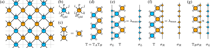
Figure 5: The iPEPS ansatz, the transfer matrix, and the fixed points. (a) The iPEPS ansatz for variational optimization. (b) The two tensors parameterizing the iPEPS. (c) The double tensor of $A$ and the double tensor of $B$ is similar. (d) The transfer matrix of the iPEPS. (e) The fixed point equation for the left fixed point $\sigma_{L}$. (f) The fixed point equation for the right fixed point $\sigma_{R}$. (g) The relation between left and right fixed points.

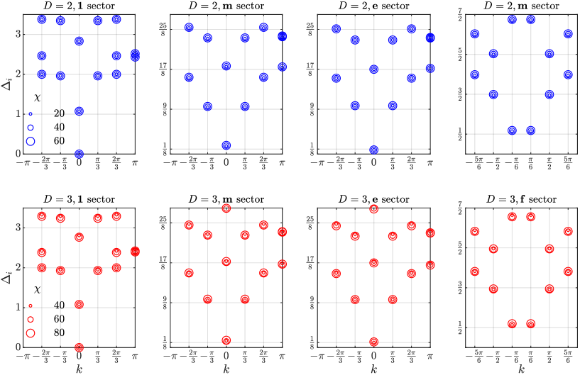
Figure 6: Finite bond dimension effect of the ES. The ES is obtained at $h_{x}=h_{z}=0.16$ from the MPO with the circumference $2N=12$ and the physical (virtual) bond dimension $D$ ($\chi$).

Figure 7: Finite circumference effect of the ES. The ES is obtained at $h_{x}=h_{z}=0.16$ from MPO with the circumference $2N$ and the physical (virtual) bond dimension $D$ ($\chi=40$).

Appendix E Tensor network method for calculating the subblock entanglement spectrum of the $\mathbb{Z}_{2}$ GH model

In this section, we show how to calculate the entanglement spectrum of the subblock reduced density matrix $\rho_{\text{GH},\boldsymbol{x}}$ of the $\mathbb{Z}_{2}$ GH model from the transfer matrix fixed points of the TC model. According to Eq. (19), $\rho_{\text{GH},\boldsymbol{x}}$ and $\rho_{\text{TC},\boldsymbol{x}}$ have the same spectrum, so we just consider $\rho_{\text{TC},\boldsymbol{x}}$, which is the reduced density matrix of $P_{\boldsymbol{x}}\ket{\Psi_{\text{TC}}}$. Because $\Tr_{L}P_{\boldsymbol{x}}\ket{\Psi_{\text{TC}}}\bra{\Psi_{\text{TC}}}P_{\boldsymbol{x}}=\left(\Tr_{L}\bra{\boldsymbol{x}}\ket{\Psi_{\text{TC}}}\bra{\Psi_{\text{TC}}}\ket{\boldsymbol{x}}\right)\otimes\ket{\boldsymbol{x}}\bra{\boldsymbol{x}}$, we can ignore $\ket{\boldsymbol{x}}\bra{\boldsymbol{x}}$ which doesn’t affect the entanglement space. Notice that $\bra{\boldsymbol{x}}\ket{\Psi_{\text{TC}}}$ can be decomposed into three parts:

$$\bra{\boldsymbol{x}}\ket{\Psi_{\text{TC}}}=\Psi_{L}T^{\boldsymbol{x}}_{A}\Psi_{L}^{\dagger}=\vbox{\hbox{ \includegraphics{three_parts.pdf}}},$$ (46)

where $\Psi_{L}$ is a matrix whose row index is the collection of all physical indices at $\partial L$ and column index is the collection of all virtual indices at the entanglement cut. Reshaping a column of $A$ tensors whose physical indices are fixed to eigenstates of $X$ operator to a matrix gives rise to $T^{\boldsymbol{x}}_{A}$. From the relation shown in Fig. 5e, we have $\Tr_{L}\bra{\boldsymbol{x}}\ket{\Psi_{\text{TC}}}\bra{\Psi_{\text{TC}}}\ket{\boldsymbol{x}}=\Psi^{*}_{L}T^{\boldsymbol{x}\dagger}_{A}\sigma_{L}T^{\boldsymbol{x}}_{A}\Psi_{L}^{\text{T}}$, because $\Psi_{L}^{\dagger}\Psi_{L}=(\mathbb{T}_{A}\mathbb{T}_{B})^{\infty}=\sigma_{L}$. Moreover, according to the method deriving effective reduced density matrix of PEPS [26], we can construct an isometric operator $\mathcal{V}=(\sigma_{L}^{-1/2})^{*}{\Psi}_{L}^{\text{T}}$ applying on physical edge degrees of freedom in $(R-\partial R)$ such that

$$\mathcal{V}\Psi^{*}_{L}T^{\boldsymbol{x}\dagger}_{A}\sigma_{L}T^{\boldsymbol{x}}_{A}\Psi_{L}^{\text{T}}\mathcal{V}^{\dagger}=(\sigma_{L}^{-1/2})^{*}{\Psi}_{L}^{\text{T}}\Psi_{L}^{*}T^{\boldsymbol{x}\dagger}_{A}\sigma_{L}T^{\boldsymbol{x}}_{A}\Psi_{L}^{\text{T}}{\Psi}_{L}^{*}(\sigma_{L}^{-1/2})^{\text{T}}=\sqrt{\sigma_{L}^{\text{T}}}T_{A}^{\boldsymbol{x}\dagger}\sigma_{L}T^{\boldsymbol{x}}_{A}\sqrt{\sigma^{\text{T}}_{L}}\sim T_{A}^{\boldsymbol{x}\dagger}\sigma_{L}T^{\boldsymbol{x}}_{A}\sigma^{\text{T}}_{L}=\sigma_{\boldsymbol{x}},$$ (47)

where we use the relation $\sigma_{L}=\sigma_{L}^{\dagger}$. So the spectrum of $\rho_{\text{GH},\boldsymbol{x}}$ and the spectrum of the operator $\sigma_{\boldsymbol{x}}$ are equal up to a normalization factor, and the subblock entanglement spectrum of the $\mathbb{Z}_{2}$ gauge Higgs model can be extracted from the PEPS of the toric code model. When considering the topological sectors of the entanglement spectrum of the $\mathbb{Z}_{2}$ GH model, we just add the defects and projects, similar to the toric code case shown in Eq. (44). In the next section, we use the operator $\sigma_{\boldsymbol{x}}$ to extract the total and distillable Rényi entanglement entropies of the $\mathbb{Z}_{2}$ GH model.

Appendix F Tensor network method for calculating the distillable Rényi entanglement entropy

This section shows how to calculate the distillable Rényi entanglement entropy using tensor networks. It is not straightforward to find the Rényi generalization of the distillable von Neumann entanglement entropy. Fortunately, Ref. [35] provides the definition of the distillable Rényi entanglement entropy:

$$S_{n}(\rho)=\frac{1}{1-1/n}\log\sum_{\boldsymbol{x}}p_{\boldsymbol{x},n}^{1/n}+S_{D,n},\quad\quad S_{D,n}=\frac{n}{1-n}\log\sum_{\boldsymbol{x}}p_{\boldsymbol{x}}\exp\left[\frac{1-n}{n}S_{n}(\rho_{\boldsymbol{x}})\right],$$ (48)

where $p_{\boldsymbol{x},n}=\Tr\bra{\boldsymbol{x}}\rho^{n}\ket{\boldsymbol{x}}/\Tr\rho^{n}$. For $n=1/2$, we have a simplified expression:

$$S_{D,1/2}=\log\sum_{\boldsymbol{x}}p_{\boldsymbol{x}}\exp[S_{1/2}(\rho_{R,\boldsymbol{x}})]=\log\sum_{\boldsymbol{x}}p_{\boldsymbol{x}}\exp[2\log\frac{\Tr(\sqrt{\sigma_{\boldsymbol{x}}})}{\sqrt{\Tr\sigma_{\boldsymbol{x}}}}]=\log\sum_{\boldsymbol{x}}\frac{\Tr\sigma_{\boldsymbol{x}}}{\sum_{\boldsymbol{x}^{\prime}}\Tr\sigma_{\boldsymbol{x}^{\prime}}}\frac{\left(\Tr\sqrt{\sigma_{\boldsymbol{x}}}\right)^{2}}{\Tr\sigma_{\boldsymbol{x}}}=\log\frac{\sum_{\boldsymbol{x}}\left(\Tr\sqrt{\sigma_{\boldsymbol{x}}}\right)^{2}}{\sum_{\boldsymbol{x}}\Tr\sigma_{\boldsymbol{x}}},$$ (49)

where $\sigma_{\boldsymbol{x}}$ is defined in Eq. (47).

Next, as a warm-up, we show the tensor network method we use to calculate the total Rényi entanglement entropy [39]. We consider the total Rényi entanglement entropy of $\boldsymbol{1}$ sector, and the Rényi entanglement entropy of other sectors can be calculated in the same way. The $1/2$-Rényi entanglement entropy is given by:

$$S_{1/2}=2\log\Tr\sigma^{1/2}_{\boldsymbol{1}}-\log\Tr\sigma_{\boldsymbol{1}}=2\log\sum_{\boldsymbol{x}}\Tr\left(P_{+}T_{A}^{\boldsymbol{x}\dagger}\sigma_{L}T^{\boldsymbol{x}}_{A}\sigma^{\text{T}}_{L}\right)^{1/2}-\log\sum_{\boldsymbol{x}}\Tr\left(P_{+}T_{A}^{\boldsymbol{x}\dagger}\sigma_{L}T^{\boldsymbol{x}}_{A}\sigma^{\text{T}}_{L}\right).$$ (50)

Because we impose the square lattice symmetry to real iPEPS tensors, we have $\sigma_{L}=\sigma_{L}^{\text{T}}$ and $T_{A}^{\boldsymbol{x}}=(T_{A}^{\boldsymbol{x}})^{\dagger}$. So, the above relation can be simplified as

$$S_{1/2}=2\log\sum_{\boldsymbol{x}}\Tr\left(P_{+}\sigma_{L}T^{\boldsymbol{x}}_{A}\right)-\log\sum_{\boldsymbol{x}}\Tr\left(P_{+}\sigma_{L}T^{\boldsymbol{x}}_{A}\sigma_{L}T^{\boldsymbol{x}}_{A}\right).$$ (51)

The terms in the above equation can be expressed as tensor networks:

$$\sum_{\boldsymbol{x}}\Tr(P_{+}\sigma_{L}T_{A}^{\boldsymbol{x}})=\frac{1}{2}\underset{\vdots}{\overset{\vdots}{\vbox{\hbox{ \includegraphics{Trace_rho_half.pdf}}}}}=\frac{1}{2}\Tr\mathcal{T}_{\text{half}}^{N},\quad\quad\sum_{\boldsymbol{x}}\Tr(P_{+}\sigma_{L}T_{A}^{\boldsymbol{x}}\sigma_{L}T_{A}^{\boldsymbol{x}})=\frac{1}{2}\underset{\vdots}{\overset{\vdots}{\vbox{\hbox{ \includegraphics{Trace_rho.pdf}}}}}=\frac{1}{2}\Tr\mathcal{T}^{N},$$ (52)

where $\mathcal{T}_{\text{half}}$ ($\mathcal{T}$) is a transfer matrix shown in the dotted blue line box in the first (second) equation. So the $1/2$-Rényi entanglement entropy can be expressed as

$$S_{1/2}=2\log\Tr\mathcal{T}_{\text{half}}^{N}-\log\Tr\mathcal{T}^{N}-\log 2.$$ (53)

When the circumference is infinite, we have $\lim_{N\rightarrow\infty}\mathcal{T}^{N}=\lambda\sum_{i=1}^{d}\ket{R_{i}}\bra{L_{i}}$, where $\lambda$, $L_{i}$($R_{i}$) and $d$ are the dominant eigenvalue, the $i$-th left (right) dominant eigenvectors and the degeneracy of dominant eigenvalue, respectively. Notice that the dominant eigenvectors satisfy the bi-orthonormal condition $\innerproduct{L_{i}}{R_{j}}=\delta_{i,j}$. Analogy we have $\lim_{N\rightarrow\infty}\mathcal{T}_{\text{half}}^{N}=\lambda_{\text{half}}\sum_{i=1}^{d_{\text{half}}}\ket{R_{\text{half},i}}\bra{L_{\text{half},i}}$. So if $N$ is very large, we have

$$S_{1/2}\approx N\log(\lambda_{\text{half}}^{2}/\lambda)+\log(d^{2}_{\text{half}}/d)-\log 2.$$ (54)

Usually, in the topological phase, $d_{\text{half}}=d=1$, so we know the TEE is $\log 2$.

Following the same logic, let us consider the distillable Rényi entanglement entropy in the trivial topological sector:

$$S_{D,1/2}=\log\sum_{\boldsymbol{x}}\left(\Tr P_{+}\sigma_{L}T_{A}^{\boldsymbol{x}}\right)^{2}-\log\sum_{\boldsymbol{x}}\Tr\left(P_{+}\sigma_{L}T_{A}^{\boldsymbol{x}}\sigma_{L}T_{A}^{\boldsymbol{x}}\right)$$ (55)

The first term is the following tensor network:

$$\sum_{\boldsymbol{x}}\left(\Tr P_{+}\sigma_{L}T_{A}^{\boldsymbol{x}}\right)^{2}=\frac{1}{4}\underset{\vdots}{\overset{\vdots}{\vbox{\hbox{ \includegraphics{Trace_rho_half_square.pdf}}}}}=\frac{1}{4}\Tr\mathcal{T}_{1}^{N},$$ (56)

where $\mathcal{T}_{1}$ is the transfer matrix in the $y$ direction shown in the blue box. So, the distillable entanglement can be expressed as

$$S_{D,1.2}=\log\Tr\mathcal{T}_{1}^{N}-\log\Tr\mathcal{T}^{N}-\log 2.$$ (57)

When the circumference is infinite, we have $\lim_{N\rightarrow\infty}\mathcal{T}_{1}^{N}=\lambda_{1}\sum_{i=1}^{d_{1}}\ket{R_{1,i}}\bra{L_{1,i}}$. So if $N$ is very large, we have

$$S_{D,1/2}\approx N\log(\lambda_{1}/\lambda)+\log(d_{1}/d)-\log 2,$$ (58)

and we can extract the topological correction $\log(d_{1}/d)-\log 2$ to the area law.

In the trivial phase of the TC model, the iMPO fixed point has the symmetry $Z_{D}^{\otimes N}\sigma_{L}=\sigma_{L}Z_{D}^{\otimes N}=\sigma_{L}$ [49]. When reshaping $\sigma_{L}$ in terms of iMPS, there exists a $W_{Z}$ according to the fundamental theorem of MPS [50], such that

$$\vbox{\hbox{ \includegraphics{W_z.pdf}}}.$$ (59)

Recall the definition of the red tensor in Eq. (45), the transfer matrix $\mathcal{T}$ can be expressed as a direct sum of two matrices (corresponding to the up and down bonds of the red tensors taking 0 and 1):

$$\vbox{\hbox{ \includegraphics{T.pdf}}}=\vbox{\hbox{ \includegraphics{T_Id.pdf}}}\oplus\vbox{\hbox{ \includegraphics{T_z.pdf}}},$$ (60)

which are related by a similarity transformation $W_{Z}$ and have the same spectrum. Therefore, each eigenvalue of $\mathcal{T}$ is at least $2$-fold degenerate, and $d=2$. For the same reason, it can be derived that the transfer matrix $\mathcal{T}_{1}$ can be expressed as a direct sum of four matrices

$$\vbox{\hbox{ \includegraphics{T_1.pdf}}}= \vbox{\hbox{ \includegraphics{T_1_00.pdf}}}\oplus\vbox{\hbox{ \includegraphics{T_1_01_2.pdf}}}\oplus\vbox{\hbox{ \includegraphics{T_1_10_2.pdf}}}\oplus\vbox{\hbox{ \includegraphics{T_1_11_2.pdf}}}$$ (61)

$$= \vbox{\hbox{ \includegraphics{T_1_00.pdf}}}\oplus\vbox{\hbox{ \includegraphics{T_1_01.pdf}}}\oplus\vbox{\hbox{ \includegraphics{T_1_10.pdf}}}\oplus\vbox{\hbox{ \includegraphics{T_1_11.pdf}}},$$ (62)

which have the same spectrum because they can be transformed into each other by similarity transformations. So each level of $\mathcal{T}_{1}$ is at least four-fold degenerate, and $d_{1}=4$. Substituting $d$ and $d_{1}$ into Eq. (58), it can be derived that distillable Rényi TEE is 0 in the trivial phase.

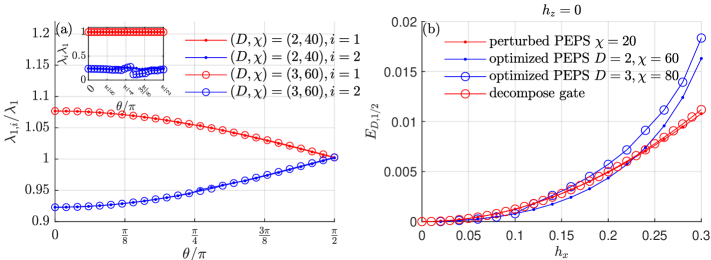
Figure 8: Detailed analysis of the distillable entanglement entropy. (a) The first two dominant eigenvalues $\lambda_{1,1}$ and $\lambda_{1,2}$ of $\mathcal{T}_{1}$ calculated for $h=0.15$. Inset: the first two dominant eigenvalues $\lambda_{1}$ and $\lambda_{2}$ of $\mathcal{T}$. (b) Comparing the density of the distillable 1/2-Rényi entanglement entropies of the exponentiated perturbed iPEPS in Eq. (68) and the variationally optimized iPEPS, as well as the rough estimation from gate decomposition in Eq. (71).

Let us consider the pure gauge theory without matter field ($h_{z}=0$) in the deconfined phase, which corresponds to the toric code phase. Different from the trivial phase, the iMPO fixed point has the symmetry $Z^{\otimes N}\sigma_{L}=\sigma_{L}Z^{\otimes N}\neq\sigma_{L}$ [49], by applying the fundamental theorem of MPS, it can be found that:

$$\vbox{\hbox{ \includegraphics{V_R_Z_2_1.pdf}}}=\vbox{\hbox{ \includegraphics{V_R_Z_2_2.pdf}}}.$$ (63)

Moreover, in the pure $\mathbb{Z}_{2}$ gauge theory, we have the $\mathbb{Z}_{2}$ 1-form symmetry $W^{X}_{\tilde{C}}=\prod_{e\in\tilde{C}}X_{e}$ on the physical level, which is equivalent to a closed loop of $Z_{D}$ operators in the virtual level of PEPS. Based on this observation, it is reasonable to assume that the PEPS tensor satisfies the following relation:

$$\vbox{\hbox{ \includegraphics{ZZ_X_relation.pdf}}}.$$ (64)

From Eqs. (63) and (64), it can be found that the terms in Eq. (61) are related by the similarity transformations

$$\vbox{\hbox{ \includegraphics{T_1_00.pdf}}}=\vbox{\hbox{ \includegraphics{T_1_11_3.pdf}}},\quad\vbox{\hbox{ \includegraphics{T_1_10_2.pdf}}}=\vbox{\hbox{ \includegraphics{T_1_01_3.pdf}}}.$$ (65)

So each level of $\mathcal{T}_{1}$ is two-fold degenerate, and $d_{1}=2$. Because in the deconfined phase $Z^{\otimes N}\sigma_{L}\neq\sigma_{L}$, the dominant eigenvalue of $\mathcal{T}$ is not necessarily degenerate, and $d=1$. From Eq. (58), we have distillable Rényi TEE is zero for pure $\mathbb{Z}_{2}$ gauge theory in the deconfined phase. In addition, if we turn on gauge-matter coupling $h_{z}$, the model does not have explicit 1-form symmetry, and the Eq. (64) is not valid anymore. So the spectrum of $\mathcal{T}_{1}$ is not necessarily degenerate and $d_{1}=1$. Substituting to Eq. (58), we know that the distillable Rényi TEE is $\log 2$ for the deconfined $\mathbb{Z}_{2}$ gauge theory coupled to the matter field.

We calculate the first and the second dominant eigenvalues of $\mathcal{T}_{1}$ and $\mathcal{T}$ along $h=0.15$, as shown in Fig. 8a. It can be found that when $\theta\neq\pi/2$ ($h_{z}\neq 0$), both the dominant eigenvalues of $\mathcal{T}$ and $\mathcal{T}_{1}$ are not degenerate, so $d_{1}=d=1$, and the distillable Rényi TEE is $\log 2$, according to Eq. (58). When $\theta=\pi/2$, the dominant eigenvalues of $\mathcal{T}_{1}$ becomes 2-fold degenerate, so $d_{1}=2$ and $d=1$, and distillable Rényi TEE is $0$, according to Eq. (58). Notice that dominant eigenvalues of $\mathcal{T}$ and $\mathcal{T}_{1}$ are very close, from Eq. (58), it implies that the density of the distillable Rényi entanglement entropy is very small. The numerical results are consistent with the theoretical analysis.

Appendix G Analysis the ground state distillable entanglement entropy of the $\mathbb{Z}_{2}$ GH model

In this section, we use tensor networks to provide the physical pictures explaining the reason that the distillable entanglement entropy can be non-zero for the pure $\mathbb{Z}_{2}$ gauge theory and also explaining the origin of the $\log 2$ topological correction to the distillable entanglement entropy in the deconfined phase with non-zero gauge-matter coupling. According to Eq. (19), the distillable entanglement entropy of a ground state of the $\mathbb{Z}_{2}$ GH model can be obtained from the corresponding ground state of the TC model via fixing physical degrees of freedom in $\partial R$. So, in order to analyze the distillable entanglement entropy of the $\mathbb{Z}_{2}$ GH model, we start from the so-called double-line PEPS representation of a TC ground state at $h_{x}=h_{z}=0$  [45]:

$$\ket{\text{TC}}=\vbox{\hbox{ \includegraphics{Pulling_through.pdf}}},$$ (66)

where the tensors are defined by Eq. (21) and a $\mathbb{Z}_{2}$ string operator of $X$ at the virtual level can pull through freely, which is a necessary condition for an iPEPS having the $\mathbb{Z}_{2}$ topological order [51, 52].

First, we consider the distillable entanglement entropy for the pure gauge theory, and Ref. [15] conjectures that it is always zero. However, in our calculation, we find that it can be non-zero, so we need to analyze it more carefully and understand why it can be non-zero. Since it is hard to analytically analyze the variationally optimized iPEPS, we can consider the wavefunction from the second-order perturbation theory:

$$|\Psi_{\text{TC}}(h_{x},0)\rangle=\left(1+\frac{h_{x}}{4}\sum_{e}X_{e}+\frac{h_{x}^{2}}{16}\sum_{(e,e^{\prime})\notin p}X_{e}X_{e^{\prime}}+\frac{h_{x}^{2}}{8}\sum_{(e,e^{\prime})\in p}X_{e}X_{e^{\prime}}+O(h_{x}^{3})\right)\ket{\text{TC}},$$ (67)

where $(e,e^{\prime})\in p$ [$(e,e^{\prime})\notin p$] means two edges $e$ and $e^{\prime}$ that do [not] belong to the same plaquette. However, the perturbed wavefunction cannot be directly transformed into an iPEPS, and it is not convenient. Using the relation $e^{x}=1+x+x^{2}/2+O(x^{3})$, we can exponentiate the terms in the perturbed wavefunction such that Eq. (67) can be expressed as [53]:

$$|\Psi_{\text{TC}}(h_{x},0)\rangle=\left[\prod_{e}\exp(\frac{h_{x}}{4}X_{e})\prod_{\langle ee^{\prime}\rangle\in p}\exp(\frac{h_{x}^{2}}{16}X_{e}X_{e^{\prime}})+O(h_{x}^{3})\right]\ket{\text{TC}}.$$ (68)

Ignoring the terms in $O(h_{x}^{3})$, $|\Psi_{\text{TC}}(h_{x},0)\rangle$ can be exactly expressed as an iPEPS.

Let us first ignore $O(h_{x}^{2})$ terms, i.e., considering $|\tilde{\Psi}_{\text{TC}}(h_{x},0)\rangle=\prod_{e}\exp(h_{x}X_{e}/4)\ket{\text{TC}}$. When fixing the physical degrees of freedom in $\partial R$, it can be found that the iPEPS is factorized into disconnected parts:

$$P_{\boldsymbol{x}}|\tilde{\Psi}_{\text{TC}}(h_{x},0)\rangle=P_{\boldsymbol{x}}\prod_{e}\exp(\frac{h_{x}}{4}X_{e})\ket{\text{TC}}=\vbox{\hbox{ \includegraphics{Measure_exp_X.pdf}}}=\vbox{\hbox{ \includegraphics{Measure_exp_X_2.pdf}}}.$$ (69)

So we have $S(\rho_{\text{GH},\boldsymbol{x}})=S(\rho_{\text{TC},\boldsymbol{x}})=0,\forall\boldsymbol{x}$, where $\rho_{\text{TC},\boldsymbol{x}}=\Tr_{L}\left[P_{\boldsymbol{x}}\ket{\tilde{\Psi}_{\text{TC}}}\bra{\tilde{\Psi}_{\text{TC}}}P_{\boldsymbol{x}}\right]/p_{\boldsymbol{x}}$ and $p_{\boldsymbol{x}}=\bra{\tilde{\Psi}_{\text{TC}}}P_{\boldsymbol{x}}\ket{\tilde{\Psi}_{\text{TC}}}$, and the distillable entanglement entropy $S_{D}=\sum_{\boldsymbol{x}}p_{\boldsymbol{x}}S(\rho_{\text{GH},\boldsymbol{x}})$ is zero.

Now let us consider terms with a coefficient the $h_{x}^{2}/16$ in Eq. (68), which are two-site non-unitary gates applying within the same plaquette. When fixing the physical degrees of freedom in $\partial R$, it can be found that the iPEPS is not factorized:

$$P_{\boldsymbol{x}}\prod_{\langle e,e^{\prime}\rangle\in p}\exp(\frac{h_{x}^{2}}{16}X_{e}X_{e^{\prime}})\ket{\text{TC}}=\vbox{\hbox{ \includegraphics{Measure_exp_XX.pdf}}}=\left(\prod_{e\in\partial R}x_{e}\right)\times\vbox{\hbox{ \includegraphics{Measure_exp_XX_2.pdf}}},$$ (70)

where there are other two-site gates within the same plaquette that we do not show for simplicity. Since the two-site gates shown in Eq. (70) connects left and right parts of the factorized iPEPS in the bottom layer, the entanglement entropy of a sector $S(\rho_{\text{GH},\boldsymbol{x}})=S(\rho_{\text{TC},\boldsymbol{x}})$ as well as the distillable entanglement $S_{D}=\sum_{\boldsymbol{x}}p_{\boldsymbol{x}}S(\rho_{\text{GH},\boldsymbol{x}})$ can be non-zero. We can roughly estimate the 1/2-Rényi distillable entanglement by simply decomposing the two-site gate:

$$E_{D,1/2}=\lim_{N\rightarrow\infty}S_{D,1/2}/N\approx 2\log(\sqrt{\frac{\cosh^{2}(h_{x}^{2}/16)}{\cosh(h_{x}^{2}/8)}}+\sqrt{\frac{\sinh^{2}(h_{x}^{2}/16)}{\cosh(h_{x}^{2}/8)}})$$ (71)

where the hyperbolic functions are from $\exp(h_{x}^{2}X_{1}X_{2}/16)=\cosh(h_{x}^{2}/16)+\sinh(h_{x}^{2}/16)X_{1}X_{2}$.

We also numerically calculate the distillable entanglement entropy of the perturbed iPEPS $\ket{\Psi_{\text{GH}}(h_{x},0)}=V\ket{\Psi_{\text{TC}}(h_{x},0)}$ using a boundary iMPS with a bond dimension $\chi=20$, where $V$ is given in Eq. (2) and $\ket{\Psi_{\text{TC}}(h_{x},0)}$ is shown in Eq. (68) [$O(h^{3})$ terms are ignored]. The result is shown in Fig. 8b, where we also compare with the results of the variationally optimized iPEPS and the rough estimation from in Eq. (71). It can be found that the dominant part of the distillable entanglement of the perturbed iPEPS in Eq. (68) is indeed from these two-site non-unitary gates, and for small $h_{x}$, the results of the variationally optimized iPEPS and the perturbed iPEPS are comparable. Because the non-zero distillable entanglement comes from the upper layer non-unitary gates, and the virtual $\mathbb{Z}_{2}$ string operator in the bottom layer disappears at the entanglement cut when pulling through from the left part to the right part, as shown in Eq. (70), $S(\rho_{\text{TC},\boldsymbol{x}})$ satisfies the area law without a topological correction: $S(\rho_{\text{TC},\boldsymbol{x}})=c_{\boldsymbol{x}}N,\forall\boldsymbol{x}$, where $c_{\boldsymbol{x}}$ is a non-universal coefficient. Hence the distillable entanglement entropy $S_{D}$ also satisfies area law without a topological correction: $S_{D}=\left(\sum_{\boldsymbol{x}}p_{\boldsymbol{x}}c_{\boldsymbol{x}}\right)N$. We conclude that the $X$ measures at $\partial R$ totally destroy the long-range entanglement along the entanglement cut. However, a portion of short-range entanglement can still be retained by the two-site non-unitary gates in the top layer.

Next, let us explain the origin of the $\log 2$ correction to the ground state distillable entanglement entropy of the $\mathbb{Z}_{2}$ GH model when the gauge-matter coupling $h_{z}$ is non-zero. It is enough to consider the case $h_{x}=0$ and $h_{z}\neq 0$, and we still analyze the ground state distillable entanglement entropy of the $\mathbb{Z}_{2}$ GH model from the corresponding ground state of the TC model. Similar to Eq. (68), we consider a first-order exponentiated perturbed iPEPS of the TC model: $\ket{\tilde{\Psi}_{\text{TC}}(0,h_{z})}=\prod_{e}\exp(h_{z}Z_{e}/4)\ket{\text{TC}}$, which is an approximate ground state of the Hamiltonian $H(0,h_{z})$ when $h_{z}$ is small. To derive the distillable entanglement entropy of $\ket{\tilde{\Psi}_{\text{GH}}(0,h_{z})}=V\ket{\tilde{\Psi}_{\text{TC}}(0,h_{z})}$, we fix the physical degrees of freedom of $\ket{\Psi_{\text{TC}}(0,h_{z})}$ at $\partial R$:

$$P_{\boldsymbol{x}}\prod_{e}\exp(\frac{h_{z}}{4}Z_{e})\ket{\text{TC}}=\vbox{\hbox{ \includegraphics{Measure_exp_Z.pdf}}}=\vbox{\hbox{ \includegraphics{Measure_exp_Z_2.pdf}}}=\vbox{\hbox{ \includegraphics{Measure_exp_Z_3.pdf}}},$$ (72)

where $M_{x_{e}}=\frac{1}{\sqrt{2}}\left(\begin{array}[]{cc}\exp(h_{z}/4)&x_{e}\exp(-h_{z}/4)\\ x_{e}\exp(-h_{z}/4)&\exp(h_{z}/4)\end{array}\right)$. When $h_{z}=0$, $M_{x_{e}}=\sqrt{2}\ket{x_{e}}\bra{x_{e}}$, so the iPEPS in Eq. (72) factorizes into two parts, and $S(\rho_{\text{GH},\boldsymbol{x}})=S(\rho_{\text{TC},\boldsymbol{x}})=0$. However, when $h_{z}\neq 0$, the iPEPS in Eq. (72) doesn’t factorize, so the virtual $\mathbb{Z}_{2}$ symmetry string operator does not disappear at the entanglement cut and can pull through from left to right, which are necessary conditions for the iPEPS in Eq. (72) possessing the long-range entanglement at the entanglement cut. From the calculation based the perturbation theory in Ref. [15], $S(\rho_{\text{GH},\boldsymbol{x}})=S(\rho_{\text{TC},\boldsymbol{x}})=c_{\boldsymbol{x}}N-\log 2$ when $h_{z}\neq 0$. So the distillable entanglement entropy of $\ket{\tilde{\Psi}_{\text{GH}}(0,h_{z})}$ is $S_{D}=\sum_{\boldsymbol{x}}p_{\boldsymbol{x}}S(\rho_{\text{GH},\boldsymbol{x}})=\sum_{\boldsymbol{x}}p_{\boldsymbol{x}}\left(c_{\boldsymbol{x}}N-\log 2\right)=\sum_{\boldsymbol{x}}\left(p_{\boldsymbol{x}}c_{\boldsymbol{x}}\right)N-\log 2$, where there is a $\log(2)$ topological correction. Therefore, we find that because the gauge-matter coupling terms in Eq. (1) do not commute with $P_{\boldsymbol{x}}$, which prevents the $X$ measurements at $\partial R$ from destroying the long-range entanglement along the entanglement cut. Like the $\log 2$ correction to the usual entanglement entropy, the $\log 2$ topological correction to the distillable entanglement entropy also originates from the underlying $\mathbb{Z}_{2}$ topological order.

References

Zeng et al. [2018]B. Zeng, X. Chen, D.-L. Zhou, and X.-G. Wen, Quantum information meets quantum matter – from quantum
entanglement to topological phase in many-body systems (2018), arXiv:1508.02595
[cond-mat.str-el] .
Chen et al. [2010a]X. Chen, Z.-C. Gu, and X.-G. Wen, Local unitary transformation, long-range quantum
entanglement, wave function renormalization, and topological order, Phys. Rev. B 82, 155138 (2010a).
Levin and Wen [2006]M. Levin and X.-G. Wen, Detecting topological order
in a ground state wave function, Phys. Rev. Lett. 96, 110405 (2006).
Li and Haldane [2008]H. Li and F. D. M. Haldane, Entanglement spectrum as
a generalization of entanglement entropy: Identification of topological order
in non-abelian fractional quantum hall effect states, Phys. Rev. Lett. 101, 010504 (2008).
Tupitsyn et al. [2010]I. S. Tupitsyn, A. Kitaev,
N. V. Prokof’ev, and P. C. E. Stamp, Topological multicritical point in the
phase diagram of the toric code model and three-dimensional lattice gauge
higgs model, Phys. Rev. B 82, 085114 (2010).
Kogut and Susskind [1975]J. Kogut and L. Susskind, Hamiltonian formulation
of wilson’s lattice gauge theories, Phys. Rev. D 11, 395 (1975).
Fradkin and Shenker [1979]E. Fradkin and S. H. Shenker, Phase diagrams of lattice
gauge theories with higgs fields, Phys. Rev. D 19, 3682 (1979).
Ho et al. [2015]W. W. Ho, L. Cincio, H. Moradi, D. Gaiotto, and G. Vidal, Edge-entanglement spectrum correspondence in a nonchiral topological
phase and kramers-wannier duality, Phys. Rev. B 91, 125119 (2015).
Verresen et al. [2022]R. Verresen, U. Borla,
A. Vishwanath, S. Moroz, and R. Thorngren, Higgs condensates are symmetry-protected topological phases: I.
discrete symmetries (2022), arXiv:2211.01376 [cond-mat.str-el]
.
Donnelly [2012]W. Donnelly, Decomposition of
entanglement entropy in lattice gauge theory, Phys. Rev. D 85, 085004 (2012).
Van Acoleyen et al. [2016]K. Van Acoleyen, N. Bultinck, J. Haegeman,
M. Marien, V. B. Scholz, and F. Verstraete, Entanglement of distillation for lattice gauge theories, Phys. Rev. Lett. 117, 131602 (2016).
Casini et al. [2014]H. Casini, M. Huerta, and J. A. Rosabal, Remarks on entanglement entropy for
gauge fields, Phys. Rev. D 89, 085012 (2014).
Buividovich and Polikarpov [2008]P. Buividovich and M. Polikarpov, Entanglement entropy
in gauge theories and the holographic principle for electric strings, Physics Letters B 670, 141 (2008).
Wu et al. [2012]F. Wu, Y. Deng, and N. Prokof’ev, Phase diagram of the toric code model in a
parallel magnetic field, Phys. Rev. B 85, 195104 (2012).
Vidal et al. [2009]J. Vidal, S. Dusuel, and K. P. Schmidt, Low-energy effective theory of the
toric code model in a parallel magnetic field, Phys. Rev. B 79, 033109 (2009).
[23]See Supplemental Material for a detailed
derivation for the properties of the quantum channel, the derivation of the
entanglement Hamiltonians, the tensor network methods for calculating the
entanglement spectra and results, and the detailed analysis of the
distillable entanglement entropy .
Zhang et al. [2012] Y. Zhang, T. Grover, A. Turner, M. Oshikawa, and A. Vishwanath, Quasiparticle statistics and braiding from ground-state entanglement, Phys. Rev. B 85, 235151 (2012).
Note [1]For non-contractible entanglement cuts the spectra depend on
the chosen MES and the trivial MES is equivalent to a contractible
entanglement cut.
Cirac et al. [2011]J. I. Cirac, D. Poilblanc,
N. Schuch, and F. Verstraete, Entanglement spectrum and boundary theories with projected
entangled-pair states, Phys. Rev. B 83, 245134 (2011).
Corboz [2016]P. Corboz, Variational optimization
with infinite projected entangled-pair states, Phys. Rev. B 94, 035133 (2016).
Vanderstraeten et al. [2016]L. Vanderstraeten, J. Haegeman, P. Corboz, and F. Verstraete, Gradient methods for variational
optimization of projected entangled-pair states, Phys. Rev. B 94, 155123 (2016).
Crone and Corboz [2020]S. P. G. Crone and P. Corboz, Detecting a topologically ordered phase from unbiased infinite
projected entangled-pair state simulations, Phys. Rev. B 101, 115143 (2020).
Flammia et al. [2009]S. T. Flammia, A. Hamma,
T. L. Hughes, and X.-G. Wen, Topological entanglement rényi entropy and
reduced density matrix structure, Phys. Rev. Lett. 103, 261601 (2009).
Chen et al. [2010b]X. Chen, Z.-C. Gu, and X.-G. Wen, Local unitary transformation, long-range quantum
entanglement, wave function renormalization, and topological order, Phys. Rev. B 82, 155138 (2010b).
Wiseman and Vaccaro [2003]H. M. Wiseman and J. A. Vaccaro, Entanglement of
indistinguishable particles shared between two parties, Phys. Rev. Lett. 91, 097902 (2003).
Note [2] is also called accessible
entanglement entropy and is the symmetry
resolved entanglement entropy.
Barghathi et al. [2018]H. Barghathi, C. M. Herdman, and A. Del Maestro, Rényi
generalization of the accessible entanglement entropy, Phys. Rev. Lett. 121, 150501 (2018).
Zhu and Zhang [2019]G.-Y. Zhu and G.-M. Zhang, Gapless coulomb state
emerging from a self-dual topological tensor-network state, Phys. Rev. Lett. 122, 176401 (2019).
Haegeman et al. [2015a]J. Haegeman, K. Van Acoleyen, N. Schuch, J. I. Cirac, and F. Verstraete, Gauging quantum states: From global to
local symmetries in many-body systems, Phys. Rev. X 5, 011024 (2015a).
Pollmann et al. [2010]F. Pollmann, A. M. Turner, E. Berg, and M. Oshikawa, Entanglement spectrum of a topological phase in
one dimension, Phys. Rev. B 81, 064439 (2010).
Haller et al. [2023]L. Haller, W.-T. Xu,
Y.-J. Liu, and F. Pollmann, Quantum phase transition between symmetry enriched
topological phases in tensor-network states (2023), arXiv:2305.02432
[cond-mat.str-el] .
Xu et al. [2020]W.-T. Xu, Q. Zhang, and G.-M. Zhang, Tensor network approach to phase transitions of a
non-abelian topological phase, Phys. Rev. Lett. 124, 130603 (2020).
Xu et al. [2022]W.-T. Xu, J. Garre-Rubio, and N. Schuch, Complete characterization of
non-abelian topological phase transitions and detection of anyon splitting
with projected entangled pair states, Phys. Rev. B 106, 205139 (2022).
Tagliacozzo et al. [2014]L. Tagliacozzo, A. Celi, and M. Lewenstein, Tensor networks for lattice gauge
theories with continuous groups, Phys. Rev. X 4, 041024 (2014).
Xu et al. [2023]W.-T. Xu, M. Knap, and F. Pollmann, Entanglement of gauge theories: from the toric
code to the lattice gauge higgs model 10.5281/zenodo.8411049 (2023).
Xavier et al. [2018]J. C. Xavier, F. C. Alcaraz, and G. Sierra, Equipartition of the
entanglement entropy, Phys. Rev. B 98, 041106 (2018).
Gu et al. [2008]Z.-C. Gu, M. Levin, and X.-G. Wen, Tensor-entanglement renormalization group approach
as a unified method for symmetry breaking and topological phase
transitions, Phys. Rev. B 78, 205116 (2008).
Schuch et al. [2013]N. Schuch, D. Poilblanc,
J. I. Cirac, and D. Pérez-García, Topological order in the projected
entangled-pair states formalism: Transfer operator and boundary
hamiltonians, Phys. Rev. Lett. 111, 090501 (2013).
Bravyi et al. [2011]S. Bravyi, D. P. DiVincenzo, and D. Loss, Schrieffer–wolff
transformation for quantum many-body systems, Annals of Physics 326, 2793 (2011).
Yang et al. [2014]S. Yang, L. Lehman,
D. Poilblanc, K. Van Acoleyen, F. Verstraete, J. I. Cirac, and N. Schuch, Edge theories in projected entangled pair state models, Phys. Rev. Lett. 112, 036402 (2014).
Haegeman et al. [2015b]J. Haegeman, V. Zauner,
N. Schuch, and F. Verstraete, Shadows of anyons and the entanglement structure of
topological phases, Nature communications 6, 8284 (2015b).
Cirac et al. [2021]J. I. Cirac, D. Pérez-García, N. Schuch, and F. Verstraete, Matrix product states
and projected entangled pair states: Concepts, symmetries, theorems, Rev. Mod. Phys. 93, 045003 (2021).
Chen et al. [2010c]X. Chen, B. Zeng, Z.-C. Gu, I. L. Chuang, and X.-G. Wen, Tensor product representation of a topological ordered phase:
Necessary symmetry conditions, Phys. Rev. B 82, 165119 (2010c).
Schuch et al. [2010]N. Schuch, I. Cirac, and D. Pérez-García, Peps as ground states: Degeneracy and
topology, Annals of Physics 325, 2153 (2010).
Vanderstraeten et al. [2017]L. Vanderstraeten, M. Mariën, J. Haegeman,
N. Schuch, J. Vidal, and F. Verstraete, Bridging perturbative expansions with tensor networks, Phys. Rev. Lett. 119, 070401 (2017).