Real-Time Neural Materials using Block-Compressed Features

Abstract

Neural materials typically consist of a collection of neural features along with a decoder network. The main challenge in integrating such models in real-time rendering pipelines lies in the large size required to store their features in GPU memory and the complexity of evaluating the network efficiently. We present a neural material model whose features and decoder are specifically designed to be used in real-time rendering pipelines. Our framework leverages hardware-based block compression (BC) texture formats to store the learned features and trains the model to output the material information continuously in space and scale. To achieve this, we organize the features in a block-based manner and emulate BC6 decompression during training, making it possible to export them as regular BC6 textures. This structure allows us to use high resolution features while maintaining a low memory footprint. Consequently, this enhances our model’s overall capability, enabling the use of a lightweight and simple decoder architecture that can be evaluated directly in a shader. Furthermore, since the learned features can be decoded continuously, it allows for random $uv$ sampling and smooth transition between scales without needing any subsequent filtering. As a result, our neural material has a small memory footprint, can be decoded extremely fast adding a minimal computational overhead to the rendering pipeline.

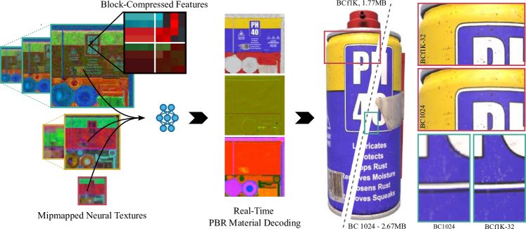
Figure 1: PBR material information is decoded in real-time from our Block Compressed neural features (BCf) resulting in an image that is visually sharper than standard BC textures of similar size.

1 Introduction

The continuous challenge of real-time rendering systems is to improve the graphics quality while reducing both the memory cost and the evaluation time. Recent progress in graphics hardware and rendering algorithms has gotten us closer to this goal. For instance, hardware accelerated raytracing [16] facilitates real-time dynamic global illumination and drastically improves the quality of shadows, reflections and refractions [42, 31, 13]. Besides that, micropolygon-based data structures [24, 20] allows the rendering of extremely detailed and dense scenes.

In terms of visual aesthetics, the Physically Based Rendering (PBR) framework has been the standard in real-time applications for well over a decade [25, 26, 17]. In this framework, a material is composed of multiple texture layers (such as albedo, normals, metalness, etc.) with each layer serving a distinct role in accurately representing various aspects of the material’s visual characteristics. Enhancing the visual quality of materials typically involves the process of either layering multiple elements [18] or increasing the texture resolution which affects their computational cost and memory footprint respectively. Consequently, rendering hyper-realistic materials in real-time applications, such as video games, remains somewhat restricted.

Recent work has shown the potential of neural networks to model and represent material properties [35, 46, 15, 44]. This neural approach aims at replacing traditional PBR textures with a collection of learned latent features, also known as neural textures [38], alongside a neural network, usually a Multi-Layer Perceptron (MLP). In this context, the network plays a crucial role in decoding the learned information and reconstructing the original material. While neural approaches have proven successful in accelerating the rendering of complex appearances [45] and compressing high-resolution PBR materials [39], its integration in real-time applications such as video games is rather complex.

There are two primary challenges that contribute to this complexity. First, the latent features have a relatively big memory footprint as they are often stored in GPU memory using an uncompressed format. Recently, Vaidyanathan et al. [39] proposed to overcome this issue by reducing the resolution and heavily quantize the values of these features. To compensate, the associated neural network tend to be large and thus computationally intensive, resulting in relatively slow evaluation time. As a result, achieving real-time performance remains challenging, and usually requires high-end hardware setups and vendor-specific extensions.

The method we present addresses these challenges. Our goal is to design a neural material model that can be integrated into a rendering pipeline without relying on any vendor-specific features and achieve real-time performance on consumer-grade hardware. To do so, we present a framework capable of (1) learning the material information at any point and scale and (2) leveraging hardware-based Block Compression (BC) format to store the learned neural features. Our features can thus be decoded continuously at any scale in $uv$ space, making it possible to reconstruct the material information with one sample per pixel and achieve smooth transition between various scales. This removes the need for any subsequent filtering step. Furthermore, encoding our neural features as regular block compressed textures reduces their memory footprint enabling us to increase their resolution. This, in turn, directly influences the complexity of the decoder network, making it considerably simpler and significantly reduces computational time.

The paper is organized as follows. Section 2 quickly details existing material representation and compression methods. We then present the technical aspects of our neural material learning framework and block based features in sections 3 and 4 respectively. In section 5 we describe how to practically use our framework to learn a standard PBR material and integrate it in a real-time rendering pipeline. Finally, we present our results in section 6 and conclude by discussing some limitations and future work in section 7.

2 Related Work

This section provides an overview of the various methods to represent and store materials that are relevant to our work. We first focus on the traditional texture based approaches (sec. 2.1) then highlight the more recent field of neural representation methods (sec. 2.2).

2.1 Texture Materials

The material properties of a three-dimensional object can be thought of as a multi-dimensional signal, which associates every point $(u,v)$ on its two-dimensional surface with the parameter space of its appearance model. In a real-time rendering context, this is primarily done via texture mapping [4] where the material properties are discretely stored in a collection of textures with dimensions $h\times w\times c$. Here, $h$ and $w$ denote the spatial resolution of the textures, and $c$ represents the total number of channels across all texture layers in the set. Increasing the visual fidelity of materials primarily relies on either adding more layers [17] or increasing their resolution which has led to a significant rise in memory requirements. To address this issue, textures are stored in GPU memory in a compressed format. Due to the object’s arbitrary position and orientation, material information are sampled from the textures at random locations. It is therefore necessary for the texture’s compression format to allow for random-access and filtering so that the information can be decompressed at any point in $uv$ space when needed in real-time. This makes standard image compression techniques, such as JPEG [40, 5] as well as newer neural based ones [6, 10] not suitable for this application as they require unpacking the entire image before being able to access pixel information.

For real-time rendering, block compression methods [7, 19] have long been the standard for compressing material textures. There are seven variants of the BC format (BC1-BC7) supported in DirectX [2], each designed for specific types of image data. All BC formats divide the image into block of 4x4 pixels and operate under the assumption that the colors in each block exhibits minimal variation and are evenly distributed along one or more line segments within the RGB color space. This means that each block can be represented by a very small color palette. In this context, the information in each block is encoded by storing the two endpoints of each segment and indexing each pixel according to its position in the RGB space (fig. 2).

Figure 2: Block Compression algorithms encode a block of $4\times 4$ pixels with a set of endpoints forming one or multiple line segments and index each pixel based on it’s projected position in the RGB space. In the case where two or more line segments are stored, the pixels are separated into groups according to a pre-defined partition $P$.

Reconstructing the pixel value is simply done by blending the two endpoints proportionally to the index value. The more recent BC6 and BC7 formats are the ones using more than one segment per block. These formats, designed for floating points and RGBA data respectively, improve the compression quality by separating the pixels inside a block into several groups, each having its own set of endpoints. The groups are chosen from a set of predefined partitions. In this case, each block stores more than one set of endpoints as well as the partition number. However, BC formats can only compress textures with up to four channels which is not suited for high dimensional materials. To overcome this, the material data is separated into several textures that are compressed independently. ASTC [30] is another popular block-based texture compression technique. It is more flexible than BC as it supports various block dimensions including non-square blocks and can even handle 3D textures.

2.2 Neural Materials

Over the last few years, advancement in neural rendering [37] have shown that it is possible to represent a digital signal, such as a material $M$, with a neural network $f_{\eta}$ by minimizing over its weights $\eta$ the following quantity:

$$\sum_{i,j}\|f_{\eta}(u_{i},v_{j})-M_{i,j}\|^{2},$$ (1)

where $M_{i,j}$ is the pixel value of the target material and $(u_{i},v_{j})$ are their corresponding local coordinates. This is an overfitting problem where the weights of the network are optimized such that the network’s output matches the target image at a given pixel. Thus, the capability of the network is key to perfectly recover the original image. For instance, simple coordinate based networks [27] are not capable of dealing with high frequency details. To improve the network’s reconstruction capacity, positional encoding [36, 11] where the input $(u,v)$ coordinates is encoded as a vector generated from a periodic function, is usually employed. However, this requires a large network to accurately reconstruct the original image which makes it not suitable for real-time evaluation. Using trainable spatial features [28, 8, 9, 34], i.e., neural textures, drastically reduces the size of the network and improves the reconstruction quality. In this setting, the input coordinates are used to sample in the neural textures using bilinear interpolation and the resulting feature vector is given as input to the neural network.

The idea of pairing a set of discrete spatial features and a neural network have proven to be popular for material representation. For instance, Rainer et al. [33] uses an encoder-decoder architecture to compress a large set of Bidirectional Texture Function layers. The encoder is trained to generate a latent code for each texel. This code is then used by the decoder, in conjunction with a light and view direction to output a single RGB value. Kuznetsov et al. [22] combined a pyramid of neural textures with a fully connected network to learn the material properties at different scales. Their model is capable of rendering materials with intricate parallax effects on an infinite plane but fails to generalize to curved surfaces. This was later done in [23]. By adding curvature and transparency as part of the network’s input and output respectively. More recently, Zeltner et al. [45] have used a set of hierarchical textures and two MLPs to bake complex film-quality appearance. Here, the first network learns the material’s reflectance and the seconds produces importance-sampled directions. This model is about three times faster than standard node-based multi-layers materials when integrated into a path-tracing pipeline.

Despite this progress, these methods often overlook the issue of storage size. In practice, learned neural features are stored in an uncompressed format which can be quite large to practically use in a real-time environment, especially when considering the memory capacity of mainstream hardware. Vaidyanathan et al [39] addressed this issue and demonstrated how neural material representations can be more efficient than standard texture compression techniques at storing PBR material information. To do so, they reduce the resolution of the neural features as much as possible and aggressively quantize their values. This made it possible to compress PBR textures at very low bit-rates, up to 0.2 bits per-pixel per-channel (bppc). However, integrating this neural material decompression in a rendering pipeline requires the use of vendor specific extensions and achieving real-time performance relies on high-end hardware. Moreover, since the model from [39] only learns the material information at fixed coordinates, it is essential to couple the neural decompression with a filtering operation [14] in order to minimize flickering and aliasing artefacts. This introduces additional computational overhead as it entails decompressing multiple samples per pixel.

In the following, we introduce a novel neural material representation using Block-compressed features (BCf) specifically designed to be integrated into a traditional real-time rendering pipeline at minimal computational overhead.

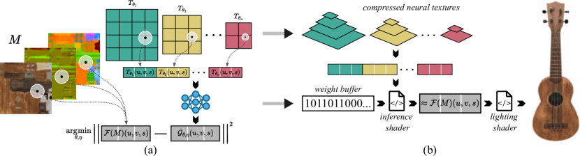
Figure 3: Overview of our neural material framework. (a) The neural features $T_{\theta_{i}}$ and the MLP $f_{\eta}$ are fitted through backpropagation to match the filtered material $\mathcal{F}(M)$. (b) After training, the neural features $T_{\theta_{i}}$ are exported as mipmapped texture sets that can be sampled by the engine and the weights $\eta$ of the MLP are exported as a binary buffer. A shader is used to perform the MLP inference after trilinearly sampling the neural texture, outputting the filtered material $\mathcal{G}_{\theta,\eta}(u,v,s)\approx\mathcal{F}(M)(u,v,s)$. Finally, The renderer can perform the shading step as usual.

3 Neural Material Framework

A PBR material $M$ is constituted of a set of properties. These properties are represented at a coordinate $(u,v)$ by a vector of dimension $c$. In a standard 3D application, this data is stored in a discrete fashion through a texture of size $w\times h\times c$ and mapped onto a 3D object. At render time, this information is sampled from the textures as follows:

$$\mathcal{F}(M)(u,v,s)\in\mathbf{R}^{c},$$ (2)

where $\mathcal{F}$ is a filtering operation and $s$ is a scale value. The filtering is essential here. It accounts for the misalignment and the difference in area between the screen pixel and its corresponding texels, caused by the 3D object’s arbitrary distance and orientation. Our neural material model aims at replacing the material textures with a set of neural features containing abstract information and a decoder network. The role of the decoder here is to reconstruct the material data at a given point and scale using the learned features. Figure 3 gives an overview of our neural material framework.

Let $\{\text{T}_{\theta_{0}},\ldots,\text{T}_{\theta_{n}}\}$ be a set of neural features of size $\left(w_{0},h_{0},d_{0}\right),\ldots,\left(w_{n},h_{n},d_{n}\right)$ with trainable parameters $\{\theta_{0},\ldots,\theta_{n}\}$. And let $f_{\eta}$ be a fully connected neural network of input size $\sum_{i=1}^{n}d_{i}$ and output size $c$ with trainable parameters $\eta$. To reconstruct the material information at a point $(u,v)$ with respect to a scale $s$, we sample each of the features, concatenate the resulting values and pass it to the neural network as follow:

$$\mathcal{G}_{\theta,\eta}(u,v,s)=f_{\eta}\left(T_{\theta_{0}}\left(u,v,s\right),\ldots,T_{\theta_{n}}\left(u,v,s\right)\right).$$ (3)

In this framework, learning the material $M$ boils down to optimizing $\theta$ and $\eta$ such that:

$$\hat{\theta},\hat{\eta}=\operatorname*{arg\,min}_{\theta,\eta}\left\|\mathcal{G}_{\theta,\eta}-\mathcal{F}(M)\right\|^{2}.$$ (4)

This allows us to train a model such that it simulates a given filtering operation. In practice, we use a batched stochastic gradient descent to perform this optimization where the gradient is computed on a batch of random values of $(u,v,s)$. This leads us to minimize the following loss:

$$\sum_{(u,v,s)\in B}\left\|\mathcal{G}_{\theta,\eta}(u,v,s)-\mathcal{F}(M)(u,v,s)\right\|^{2}.$$ (5)

Once trained, we export the learned features as textures and store the model’s weights in a binary buffer. At render time, the neural textures and the weights are used to reconstruct the material information. To make neural materials more appealing, it is important to reduce their memory footprint and to make their memory size match the traditional material texture. There are two possible strategies here. The first one consists in using a small number of low resolution neural features [39]. However, this approach leads to a more complex decoder network, making the material reconstruction more computationally expensive. The second aims at storing the neural features more efficiently by using a compression algorithm. We chose the latter and propose to store them in the BC6 format as it is designed to handle floating point data and allows for random-access. Additionally, these compressed features can be handled like any traditional texture, which considerably simplifies the neural material’s decoding at rendertime. However, naively compressing the learned features at the end of the training will lead to artifacts that severely impact the visual quality of the reconstructed material (fig. 4). In order to tackle this issue, we propose a specific block-compressed neural feature parameterization that is compatible with the BC6 format.

Figure 4: Neural material reconstructed from (a) raw unconstrained neural features and (b) compressed ones. The naive compression of the neural features will lead to artifacts severely affecting the visual quality.

4 Block Based Neural Features

In this section, we detail our block-based neural features. The goal here is to be able to store the trained neural features as BC6 textures without affecting the visual quality and use them in a real-time environment. To do so, we structure the features in blocks of $4\times 4$ and define the parameters on a per-block basis (sec. 4.1). Then, we design a forward pass that emulate the BC6 decompression (sec. 4.2) and takes advantages of hardware texture samplers (sec. 4.3). This makes it possible to directly export the neural features as BC6 textures without the need for a subsequent compression step and use them into real-time environment with a minimal computational overhead.

4.1 Block parameterization

In the BC6 setting, an image is stored by encoding the endpoints value for each $4\times 4$ block and indexing each pixel according to its distance to the corresponding line segment (fig. 2). The dual partition mode of BC6 divides the pixels inside each block into two regions allowing for two lines segments per block.

We design the neural features to mimic this behaviour. Given a feature layer $T_{\theta_{i}}$ of size $w\times h\times 3$, we force its values within a block of size $4\times 4$ to lie on two lines segments. This is done by design, we structure our block-based neural features by modeling the parameter set $\theta_{i}$ such that each block of size $4\times 4$ is modeled with

$$\begin{cases}l_{1}=\{e_{1},e_{2}\}\subset\mathbf{R}^{3}\\ l_{2}=\{e_{3},e_{4}\}\subset\mathbf{R}^{3}\\ \alpha=\{\alpha_{1},\ldots,\alpha_{16}\}\subset[0,1]\end{cases},$$ (6)

where $l_{1}$ and $l_{2}$ are two sets of endpoints for the first and second line segments respectively and $\alpha$ gives the the relative position of each one of the sixteen pixels of the block on the corresponding line segment. To determine which pixel belongs to which segment, we attach to each block an integer, $k\in\{0,\ldots,31\}$, linking to a binary mask of the corresponding partition. We refer the reader to the DirectX BC documentation [2] for all the technical details regarding the pre-defined partitions. Reconstructing the material information (eq. 3) requires sampling each neural feature $T_{\theta_{i}}$ at position $(u,v)$ and scale $s$. This consists of performing the BC6 decompression and then filtering the corresponding value according to a certain strategy (fig. 5). In order to train our block-based model, it is necessary to backpropagate through this decompression. Additionally, it is important to choose a filtering strategy that does not incur additional computation overhead. The later is crucial to be able to integrate our neural material model in rendering pipelines.

Figure 5: Evaluating $T_{\theta_{i}}$ at position $(u,v)$ and scale $s$ is done by performing a BC6 decompression then filtering the result with respect to the given scale. Our simulated BC6 decoding makes it possible to backpropagate through this operation and train the per-block neural features.

4.2 Trainable BC6 decompression

In the two partition mode, a BC6 block stores two sets of quantized endpoints, the pixel indices and a partition ID. The decompression operation uses this data to recover back the original information by mixing the endpoints proportionally with the index values. According to the BC6 standard specification [2], this operation is non-linear and is done in three steps. First, the endpoints of each block are unquantized as follow :

$$\overline{e}_{i}=\frac{a2^{16}e_{i}+2^{15}}{2^{b}},\quad i=1,\ldots,4.$$ (7)

Where $a=\nicefrac{{31}}{{64}}$ for the unsigned BC6 mode, $a=\nicefrac{{31}}{{32}}$ for the signed BC6 mode and $b$ is the number of bits used to quantize the endpoints. This essentially maps the endpoint values into a valid range. The second step consists in interpolating the endpoints linearly:

$$y=P_{k}\odot(e_{1}+2^{q}\alpha(\overline{e}_{2}-\overline{e}_{1}))+\neg P_{k}\odot(\overline{e}_{3}+2^{q}\alpha(\overline{e}_{4}-\overline{e}_{3})),$$ (8)

where $P_{k}$ is the binary mask associated with partition $k$ and $q$ is the number of bits used to quantize the relative position of a pixel on the line. This will give a value $y\in[-31743,31743]$ and whose bits are finally re-intrepreted as a half precision number [3]. This cast is a non-linear transformation that can be simulated with the following operation

$$w=2^{h(v)-14}\left(\frac{v}{1024}-h(v)\right),$$ (9)

where $h(v)=\max\left(\lfloor\nicefrac{{(v-1)}}{{1024}}\rfloor-1,0\right)$.

Therefore, to simulate the hardware BC6 decompression for each pixel within a block, we unquantize and mix the endpoints using eq. (7) and eq. (8), and finally simulate the bit re-interpretation operation with eq. (9) resulting in the final value $w$. All these operations being almost-everywhere differentiable, it allow us to backpropagate through the BC6 decompression, when the partitions are fixed.

4.3 Hardware compliant filtering

In a real-time rendering context, sampling a texture at a particular scale is often done via mipmapping. This technique consists in explicitly storing in memory a version of the texture at different scales, also known as mip, and performing trilinear filtering. This involves doing a texture lookup and bilinear filtering on the two closest mipmap levels (one higher and one lower), and then linearly interpolating the results. In general, this approach stabilizes sampling performance as it fixes the number of processed pixels for each query independently of the scale values.

Since our goal is to integrate the neural material model in a real-time environment, we propose to rely on trilinear interpolation to filter the neural features $T_{\theta_{i}}$. This makes it possible to exploit hardware accelerated texture filtering to sample the corresponding neural textures during rendering. To do so, we consider that each feature layer $T_{\theta_{i}}$ is composed of a pyramid with $S_{i}$ block-based mips, $T_{\theta_{i}}=\{T_{\theta_{i}}^{0},\ldots,T_{\theta_{i}}^{S_{i}}\}$, of decreasing sizes. Each block-based mip has independent parameters that will be adjusted during the training process. In this setting, the scale parameter $s\in[0,S_{i}]$ refers to the level at which the features $T_{\theta_{i}}$ are sampled. This is done as follows:

$$T_{\theta_{i}}(u,v,s)=\lambda T^{\lfloor s\rfloor+1}(u,v)+(1-\lambda)T^{\lfloor s\rfloor}(u,v),$$ (10)

where, $\lambda=s-\lfloor s\rfloor$ and $T_{\theta_{i}}^{k}(u,v)$ is the bilinear interpolation from the $k^{th}$ block based mip at coordinates $(u,v)$ (fig. 6).

Figure 6: When sampling a feature at a scale level $s$, the block compressed features are filtered using a trilinear interpolation. This requires sampling the two closest mip levels $\lfloor s\rfloor$ and $\lfloor s\rfloor+1$ using a bilinear interpolation than linearly mixing the results.

5 Implementation details

In this section, we present all the practical details related to the encoding and decoding of PBR material information with our block based neural features.

5.1 Material encoding

Model structure

In our implementation, we use 4 sets of neural block-based features $\{T_{\theta_{0}},T_{\theta_{1}},T_{\theta_{2}},T_{\theta_{3}}\}$ with size $w_{i}=h_{i}=2^{n_{i}}$. As described in section 4.3, each $T_{\theta_{0}}$ consists of a pyramid with several block-based mips of decreasing power of two sizes. We use a simple MLP of input size 12 and one hidden layer as our decoder network and adjust the size of the output according to the endcoded material. We have experimented with two MLP configurations with one hidden layer of size 16 and 32 respectively.

Partition selection strategy

As mentioned in section 4.2, we can backpropagate through the simulated BC6 decompression only if the partition IDs for each block are fixed. In order to maximise the reconstruction quality, it is necessary to select the most optimal partition for each block. However, choosing the one with the lowest error during training is not straightforward. Indeed, the optimal values of $l_{1}$, $l_{2}$ and $\alpha_{i}$ coefficients might vary significantly depending on which partition $k$ is considered. This means every-time the partition changes, these parameters need to re-adapt to the new set of pixels resulting in training instability. To overcome this issue, one approach would be to learn in parallel all the parameters for each possible partition for each block. This is unpractical and would increase both the memory and time needed to learn the material model. Instead of that, we propose to consider the partitions indices as hyper-parameters, and thus fix them before the training. Since randomly setting their values would possibly lead to non-optimal partition attribution, we therefore propose to learn the material model in two steps. First, we perform a quick training using a set of features with unconstrained parameters, i.e., move freely in 3D space and not constrained on a line segment. Then, we initialize the block-based features by compressing the unconstrained features with the BC6 algorithm. This provides us both a partition selection strategy and a relevant initialization of the parameters within each block. In our experiments, we train the model for 5k iterations with unconstrained parameters, then use the result to initialise the block based features. While this does not guarantee the selection of optimal partitions, we found that it improves the reconstruction quality and consistency of the results.

Reference material sampling

In our experiments, we consider reference materials with $S$ mipmaps and sample them at random during training by doing a bicubic filtering on the closest two mips than linearly interpolating the results. More precisely, we process batches of 512x512 uniformly sampled uv-grids, for each batch we also sample a continuous scale parameter $s$ uniformly in $[0,S]$ where $S$ is the number of mipmap. Both the reference material and the neural material (sec. 4.3) are then sampled at $(u,v,s)$ and the loss is computed as the mean squared error between them. For more details on the training parameters, we refer to the results in section 6.

5.2 Real-time Decoding

We export each trained feature layer as a mipmapped BC6 texture. The block-based structure of these features simplifies this operation as it only involves the quantization and encoding of the endpoints and alpha values with 6bits and 4bits respectively. The network’s weights are stored directly in a binary buffer as fp16 values since their size is negligible.

Multiple methods can be employed to integrate our model into a real-time renderer. Our implementation is rather straightforward and doesn’t require any vendor specific features. We simply load the neural textures and weights in GPU memory and proceed as follows (fig 3). First, we use the partial derivatives of the input pixel’s $uv$ coordinates to compute the sampling scale $s_{i}$ for each neural texture $T_{\theta_{i}}$

$$s_{i}=\log_{2}\left(\max\left(\left|\nicefrac{{\partial uv}}{{\partial u}}\right|,\left|\nicefrac{{\partial uv}}{{\partial v}}\right|\right)\right)+b_{i},$$ (11)

where $b_{i}=\log_{2}\left(\max(\nicefrac{{h_{i}}}{{h}},\nicefrac{{w_{i}}}{{w}})\right)$ is a bias value that depends on the neural texture’s and render resolutions, respectively $w_{i}\times h_{i}$ and $w\times h$. Then, we sample each of the neural textures using the GPU’s hardware filtering capabilities and pass the resulting values to the decoding shader. Within this shader, the sampled values processed through a sequence of functions that perform vector-matrix multiplications with the model’s weights and the return the material information. When rendering a scene with multiple neural materials, we store all the different network weights in a single buffer and use a material id value as an offset to access a specific model’s weights. Finally, the pixel is shaded.

6 Results

In this section, we demonstrate the efficiency and performance of our method on various examples. We describe our experimental setup in section 6.1, then we showcase the results in section 6.2 and the decoding time performance in section 6.3.

Figure 7: Our evaluation dataset comprise of twelve 3D objects. Our implementation can render a scene with 144 objects in real-time achieving a performance of about 200fps.

6.1 Experimental setup

Evaluation dataset

We gathered a dataset of twelve textured 3D models (fig. 7) from the public library PolyHaven [1]. The material information for each object is constituted of eight channels, and stored into three textures : albedo, normals and ARM. The resolution of each texture is $2048\times 2048$ (2K). The albedo layer has 3 channels and contains the diffuse color information. The normals layer has 2 channels and contains the x, y coordinates of the surface normals with respect to a local tangent frame. The ARM layer has 3 channels and contains the ambient occlusion, surface roughness and metalness parameters. Note that our model is not restricted to learn only this specific material representation but can handle materials with arbitrary number of layers.

Model configuration.

In our experiments, our models consisted of four mipmapped square shaped block compressed features. Table 1 details the resolution of each of the feature layers along with the corresponding number of mips. For the decoding network, we use an MLP of input size 12, output size 8 and one hidden layer of dimension 16. We use the ReLu activation function for the input and hidden layers, while the activation of the output layer is set to identity. For the rest of this paper, we will refer to our model by the name of its block compressed features configuration. For instance BCf-0.5K refers to the model with a resolution of $T_{\theta_{0}}$ equal to 512.

Table 1: Configuration of the neural block compressed features that we used for our tests

	$T_{\theta_{0}}$		$T_{\theta_{1}}$		$T_{\theta_{2}}$		$T_{\theta_{3}}$
	size	mips	size	mips	size	mips	size	mips
BCf-0.5k	512	8	256	7	128	6	64	5
BCf-1k	1024	9	512	8	256	7	128	6
BCf-2K	2048	10	1024	9	512	8	256	7

Training parameters.

We use the Adam stochastic gradient descent algorithm [21] with an exponential decay learning rate scheduler. We set a different learning rate for both the block compressed features and the MLP in order to balance the gradient backpropagation. We train the models for a total of 205k iterations in two phases. In the first phase we train our model with unconstrained features for 5k iterations using learning rates of $5\times 10^{-2}$ and $10^{-3}$ for the features and the MLP respectively, and a decay parameter $\gamma=0.9995$. The second phase starts by initializing the block compressed features from unconstrained ones. Then we train the model for 200k iterations using a learning rate of $10^{-2}$ for the features and $10^{-3}$ for the MLP with decay parameter $\gamma=0.99999$. For reference, our BCf-1K model requires about 140 minutes to be trained for the 205k iteration on an NVIDIA RTX2070 with our implementation using the PyTorch library [32]. Note that we observed that the model already outputs decent results after 10k steps, in approximately 15 minutes.

Compared methods.

We compare our method with standard BC compression, ASTC [43] and our implementation of Vaidyanathan et al.’s NTC [39]. Both BC and ASTC compressed textures were generated from NVIDIA’s texture tools exporter [29] with a compression quality set to the highest possible setting. For BC compression, we used the BC1 format to compress the albedo and ARM textures and BC5 format for the normals. This BC configuration is standard and used in most of real-time applications such as video games. For ASTC, we used a $12\times 12$ blocks as it matches the size of our BCf-1K configuration. In the context of our experiments, where the reference material resolution is $2048\times 2048$, the highest resolution of the features grid of NTC is set to 512 for NTC0.2, NTC0.5 and 1024 for NTC1.0.

Considered metrics.

Quantifying the visual quality of an image is still an open problem as no metric can effectively align with human perception. This is especially the case when the types of distortions introduced by the compression methods are different. For instance, traditional BC and ASTC methods tends to have more blocky artefacts while neural methods such as ours and NTC tend to exhibit color shift and feature bleeding. For this reason we mainly rely on the PSNR value as it is directly linked to the loss we are optimizing. In this sense, the PSNR can be seen more as a proxy for the method’s capacity to approximate the reference data and not as a measure of visual quality. We also include SSIM [41] as it tends to be more in line with human perception. We compute our metrics for each mip level and aggregate the values as described by Vaidyanathan et al. in [39].

Table 2: Evaluation of the reconstruction metrics (PSNR and SSIM) on the whole dataset. For PSNR, we averaged the mean-squared error over all the mips (as proposed in [39]) and all the models then computed the PSNR. We also put the size in megabytes (MB) for each method.

				NTC 0.2		NTC 0.5		NTC 1.0		BC		ASTC12
	BCf–0.5K	BCf–1K	BCf–2K	1spp	bilinear	1spp	bilinear	1spp	bilinear	1024	2048	1024	2048
PSNR $(\uparrow)$	28.99	31.96	35.73	20.04	32.86	30.99	34.83	26.98	37.72	30.83	37.70	28.40	32.32
SSIM $(\uparrow)$	0.84	0.90	0.95	0.90	0.90	0.92	0.93	0.95	0.96	0.88	0.97	0.83	0.91
size (MB)	0.44	1.77	7.08	0.93		2.26		4.53		2.67	10.67	0.47	1.89

6.2 Reconstruction quality

In this section, we showcase the capacity of our model to reconstruct the learned PBR material information. In a 3D setting, the material information is sampled at random $uv$ coordinates, due to the 3D object’s orientation and distance. We emulate this in our experiments by randomly sampling a point within each pixel and comparing our results with a filtered version of the reference data. In practice, this is done by adding a random noise to a regular grid of $uv$ points such that their coordinates remains within the pixel’s boundary.

Block-compressed feature.

Figure 8 shows that our training framework is capable of learning neural features that are compatible with the BC6 format. The material information reconstruction from the raw half-precision floating-point format (fp16) block features (fig. 8 (a)) and from the exported BC6 block features (fig. 8 (b)) are visually indistinguishable.

Figure 8: Effects of BC compression of the neural features on the decoded textures. The decoded textures before BC compression of the neural features (a) are not visually different from the decoded textures after BC compression (b). The render on the right shows that no artifacts are visible on the final shaded texture.

Figure 9: Reconstruction PSNR versus size in megabytes (MB) for all the methods presented in table 2.

Comparison results.

We trained all our different configurations against a reference 2K material and compared them to the methods mentioned in section 6.1. The results are gathered in table 3 and illustrated in figure 9. It is not surprising to see that the resolution of the neural features has a direct impact on the capacity of the model to reconstruct the material (see fig. 10). Compared to standard BC and ASTC textures our model yields sharper materials and does not exhibit blocky artifacts (see fig. 11). In general, our model reconstructs a slightly smoother material compared to NTC. However, NTC cannot directly handle random $uv$ samples. Its performance drops significantly when reconstructing the material with 1 sample per pixel (spp) (fig 9). Figure 12 shows that its performance is not consistent across mip level. To handle this, NTC requires to follow up the decoding step with a filtering operation which increases the number of network evaluation per pixel. For instance, it is required to decode the four neighbour pixel for bilinear filtering or the eight neighbour pixels for trilinear filtering. Our model does not suffer for this issue and is capable of reconstructing a filtered image directly form a random $uv$ value. This makes it more suitable for real-time rendering as only one network evaluation per pixel is necessary.

Figure 10: Effect of the resolution of the neural compressed features on the visual reconstruction. Note that this resolution parameter is directly linked to the compression ratio our method achieve.

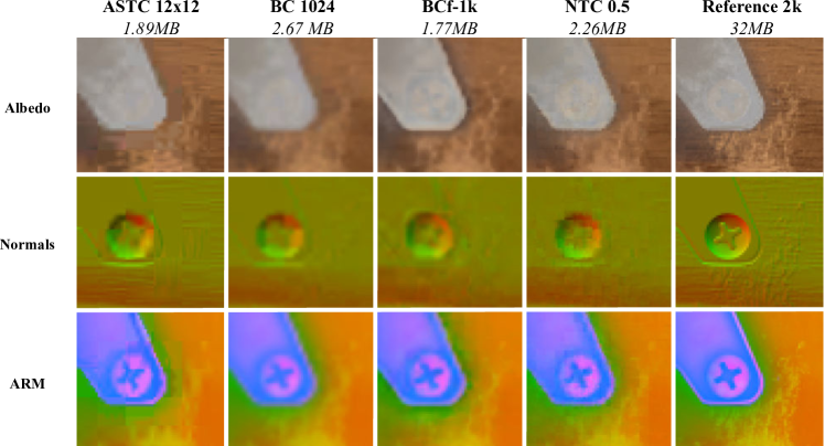
Figure 11: Close-up crop of the Ukulele model material textures. Comparison between ASTC, BC, our BCf-1K, NTC0.5 methods and the reference 2K material.

Figure 12: Evolution of the PSNR reconstruction metric over the scales on the Ukulele’s material. This demonstrates that the proposed BCf–1K method can be used at 1 sample per-pixel (spp) without the need of additional filtering.

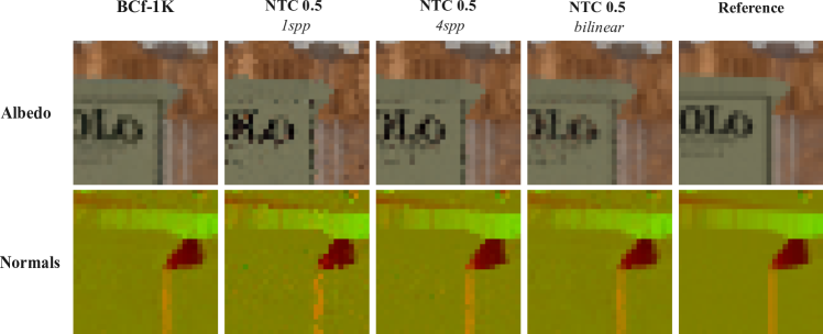
Figure 13: Visual comparison on the mip 3 between our BCf-1K method at 1 sample per-pixel (spp), the NTC method at 1 spp, 4 spp and with bilinear filter. This figure illustrates the observed behaviour in fig. 12.

6.3 Decoding performance

We created a scene consisting of 144 3D objects whose materials are encoded using our neural model. This scene can be rendered at more than 200 frames per second (fps) on a consumer-grade GPU (fig 7). In order to better illustrate the computational overhead of our neural material model, we rendered a textured full-screen quad at at $1080$p, $1440$p and $2160$p (4K) resolutions using a NVIDIA RTX2070. We then compared the total rendering time or our BCf–1K with rendering times obtained using the same setup but with standard BC textures. The results are presented in table 3. They clearly show that our method is well suited for real-time environments as the computational overhead on a 4K resolution is only 0.6ms for a full 4K screen. The small computational overhead is a direct consequence of our block compressed neural features. Exporting these features as BC6 textures makes their memory footprint small which makes it possible to increase their resolution. This allows us to rely on a very small and fast decoder network to reconstruct the material. More importantly, it enables the use of hardware texture filtering operations to sample the features at render-time which minimizes the overhead.

Table 3: Required time to render a textured full-screen quad using an NVIDIA RTX2070. For the neural material models we also show the computational overhead of evaluating the network. The time is averaged over 300 frames.

		BCf-1K
	BC Textures	total time	neural overhead
$1080$p	0.376 ms	0.555 ms	0.179 ms
$1440$p	0.614 ms	0.924 ms	0.310 ms
$2160$p	1.684 ms	2.324 ms	0.640 ms

7 Limitations and Future Work

In this section we discuss some of the limitations of our neural material model and offer avenues for future work.

Reconstruction artifacts

In some part of the reconstructed material, we experimented material’s layer bleeding and color shift. These artifacts generally affect the overall visual quality of the material. Since our model is exploiting correlation between the channels and projecting the data into a smaller dimensional space, we believe these artifacts occur when there is small correlation or their absolute values are too divergent. In addition, the use of a decoding network consisting of only one hidden layer makes our model struggle with reconstructing and separating the data from the material layer. Even increasing the network size is hardly an option considering the potential overhead, it should be possible to overcome these issues by designing a decoder network that separates the reconstruction of uncorrelated layers. In addition to that, we could learn a tone mapping operator to map each output to the corresponding values. The challenge here, is to keep the decoding network small in order to maintain real-time performance, so we leave this to future work.

Reconstructing High Frequencies

Our model may struggle to learn high-frequency details that impair the quality. This as a consequence of the features being of lower resolutions of the target reconstruction one. In this setting the decoder network must perform some super-resolution. However, we use a very shallow network, which prevent the effective use of positional encoding that could have helped bring out more high frequency information like shown in NTC. As future work, we want to investigate the usage of non square features (i.e., larger resolution in one dimension). This would allow to encode higher frequencies separately in horizontal and vertical directions while keeping the memory the same.

Faster material encoding

In the current version, our PyTorch implementation of the training pipeline requires between about 140 minutes for 200K iteration steps. For now, we mainly focused on designing a model with a fast decoder which is critical for a real-time applications such as video games. Reducing the training time is equally important as it is key to making such methods less computationally intensive and more practical in an dynamic environments where the assets keep changing. There are several avenues that we can employ to improve on this. For instance, it is possible to train a generic encoder to initialize the embedding from the reference material in order to have a better starting point and only train for a few iterations as in [45]. Additionally, we could improve the sampling strategy during training and sample only where it matters. This could also have an impact on the visual quality as the network will focus on minimizing the errors only where it matters.

Simulate more complex filtering

Our work shows that even with simple MLP decoders, our architecture is able to emulate simple texture filtering operations such as bilinear and bicubic filtering. We believe that this idea can be explored further by training models to emulate more complex filtering operators. One way to improve the filtering is to take into account anisotropy in the scale parameter. In a real-time rendering context, anisotropic filtering is done by generating non-square mipmap in each dimension. These directional mips are then sampled depending on the directional scale parameters $\nicefrac{{\partial uv}}{{\partial u}}$ and $\nicefrac{{\partial uv}}{{\partial v}}$. We plan to adapt our framework to simulate anisotropic filtering by adapting the architecture of our block-compressed feature layers. Another option we plan to explore, is the capability of learning more complex filters such that the magic kernel [12].

8 Conclusion

This work introduces a novel block-compressed feature layer along with a continuous neural material encoding framework. This allows us to design a encoding and a decoding method that fits well within the real-time rendering pipeline constraints. We demonstrate the ability of our method to compress PBR materials efficiently and decompress them in real-time in a shader on consumer-level hardware. By taking into account memory and time constraints, and by taking advantage of existing hardware operations, we make neural textures usable at large scale in a real-time rendering pipeline, such as a video game engine. We hope that our work could serve as a starting point for future work. And open the door for more complex use cases, such as learning directional materials or more complex filtering.

References

- [1] PolyHaven, https://polyhaven.com/.
- [2] Texture block compression in direct3d 11. https://learn.microsoft.com/fr-fr/windows/win32/direct3d11/texture-block-compression-in-direct3d-11. Accessed: 2023-09-28.
- [3] Ieee standard for floating-point arithmetic. IEEE Std 754-2019 (Revision of IEEE 754-2008), pages 1–84, 2019.
- [4] T. Akenine-Mller, E. Haines, and N. Hoffman. Real-Time Rendering, Fourth Edition. A. K. Peters, Ltd., 4th edition, 2018.
- [5] J. Alakuijala, R. Van Asseldonk, S. Boukortt, M. Bruse, I.-M. Com\textcommabelowsa, M. Firsching, T. Fischbacher, E. Kliuchnikov, S. Gomez, R. Obryk, et al. Jpeg xl next-generation image compression architecture and coding tools. In Applications of Digital Image Processing XLII, volume 11137, pages 112–124. SPIE, 2019.
- [6] J. Ballé, D. Minnen, S. Singh, S. J. Hwang, and N. Johnston. Variational image compression with a scale hyperprior. arXiv preprint arXiv:1802.01436, 2018.
- [7] G. Campbell, T. A. DeFanti, J. Frederiksen, S. A. Joyce, L. A. Leske, J. A. Lindberg, and D. J. Sandin. Two bit/pixel full color encoding. In ACM SIGGRAPH conference proceedings, volume 20, 1986.
- [8] A. Chen, Z. Xu, X. Wei, S. Tang, H. Su, and A. Geiger. Dictionary fields: Learning a neural basis decomposition. ACM Trans. Graph., 2023.
- [9] Z. Chen, Z. Li, L. Song, L. Chen, J. Yu, J. Yuan, and Y. Xu. Neurbf: A neural fields representation with adaptive radial basis functions. In Proceedings of the IEEE/CVF International Conference on Computer Vision, pages 4182–4194, 2023.
- [10] Z. Cheng, H. Sun, M. Takeuchi, and J. Katto. Learned image compression with discretized gaussian mixture likelihoods and attention modules. In Proceedings of the IEEE/CVF conference on computer vision and pattern recognition, pages 7939–7948, 2020.
- [11] S.-F. Chng, S. Ramasinghe, J. Sherrah, and S. Lucey. Gaussian activated neural radiance fields for high fidelity reconstruction and pose estimation. In European Conference on Computer Vision, pages 264–280. Springer, 2022.
- [12] Costella P., John. Solving the mystery of Magic Kernel Sharp. johncostella.com/magic/mks.pdf, 2021.
- [13] S. Datta, D. Nowrouzezahrai, C. Schied, and Z. Dong. Neural shadow mapping. In ACM SIGGRAPH 2022 Conference Proceedings, pages 1–9, 2022.
- [14] M. Fajardo, B. Wronski, M. Salvi, and M. Pharr. Stochastic texture filtering, 2023.
- [15] J. Fan, B. Wang, M. Hašan, J. Yang, and L.-Q. Yan. Neural layered brdfs. In Proceedings of SIGGRAPH 2022, 2022.
- [16] X. Feng. Real-time cluster path tracing for remote rendering. In ACM SIGGRAPH 2022 Courses, 2022.
- [17] S. Hill, S. McAuley, L. Belcour, W. Earl, N. Harrysson, S. Hillaire, N. Hoffman, L. Kerley, J. Patry, R. Pieké, et al. Physically based shading in theory and practice. In ACM SIGGRAPH 2020 Courses, pages 1–12. 2020.
- [18] S. Hillaire and C. de Rousier. Authoring materials that matters - substrate in unreal engine 5. In ACM SIGGRAPH 2023 Courses, 2023.
- [19] K. Iourcha, K. Nayak, and Z. Hong. System and method for fixed-rate block-based image compression with inferred pixel values, 1999.
- [20] B. Karis, R. Stubbe, and G. Wihlidal. A deep dive into nanite virtualized geometry. In ACM SIGGRAPH 2021 Courses, 2021.
- [21] D. P. Kingma and J. Ba. Adam: A method for stochastic optimization. arXiv preprint arXiv:1412.6980, 2014.
- [22] A. Kuznetsov, K. Mullia, Z. Xu, M. Hašan, and R. Ramamoorthi. Neumip: Multi-resolution neural materials. Transactions on Graphics (Proceedings of SIGGRAPH), 40(4), July 2021.
- [23] A. Kuznetsov, X. Wang, K. Mullia, F. Luan, Z. Xu, M. Hasan, and R. Ramamoorthi. Rendering neural materials on curved surfaces. In ACM SIGGRAPH 2022 conference proceedings, pages 1–9, 2022.
- [24] A. Maggiordomo, H. Moreton, and M. Tarini. Micro-mesh construction. ACM Transactions on Graphics (TOG), 42(4):1–18, 2023.
- [25] S. McAuley, S. Hill, N. Hoffman, Y. Gotanda, B. Smits, B. Burley, and A. Martinez. Practical physically-based shading in film and game production. In ACM SIGGRAPH 2012 Courses, 2012.
- [26] S. McAuley, S. Hill, A. Martinez, R. Villemin, M. Pettineo, D. Lazarov, D. Neubelt, B. Karis, C. Hery, N. Hoffman, and H. Zap Andersson. Physically based shading in theory and practice. In ACM SIGGRAPH 2013 Courses, 2013.
- [27] B. Mildenhall, P. P. Srinivasan, M. Tancik, J. T. Barron, R. Ramamoorthi, and R. Ng. Nerf: Representing scenes as neural radiance fields for view synthesis. 2020.
- [28] T. Müller, A. Evans, C. Schied, and A. Keller. Instant neural graphics primitives with a multiresolution hash encoding. ACM Trans. Graph., 41(4):102:1–102:15, July 2022.
- [29] NVIDIA. Nvidia texture tools exporter.
- [30] J. Nystad, A. Lassen, A. Pomianowski, S. Ellis, and T. Olson. Adaptive scalable texture compression. In Proceedings of the Fourth ACM SIGGRAPH/Eurographics Conference on High-Performance Graphics, pages 105–114, 2012.
- [31] Y. Ouyang, S. Liu, M. Kettunen, M. Pharr, and J. Pantaleoni. Restir gi: Path resampling for real-time path tracing. In Computer Graphics Forum, volume 40, pages 17–29. Wiley Online Library, 2021.
- [32] A. Paszke, S. Gross, F. Massa, A. Lerer, J. Bradbury, G. Chanan, T. Killeen, Z. Lin, N. Gimelshein, L. Antiga, A. Desmaison, A. Kopf, E. Yang, Z. DeVito, M. Raison, A. Tejani, S. Chilamkurthy, B. Steiner, L. Fang, J. Bai, and S. Chintala. Pytorch: An imperative style, high-performance deep learning library. In Advances in Neural Information Processing Systems 32, pages 8024–8035. Curran Associates, Inc., 2019.
- [33] G. Rainer, W. Jakob, A. Ghosh, and T. Weyrich. Neural btf compression and interpolation. In Computer Graphics Forum, volume 38, pages 235–244. Wiley Online Library, 2019.
- [34] S. Shin and J. Park. Binary radiance fields. arXiv preprint arXiv:2306.07581, 2023.
- [35] A. Sztrajman, G. Rainer, T. Ritschel, and T. Weyrich. Neural brdf representation and importance sampling. In Computer Graphics Forum, volume 40, pages 332–346. Wiley Online Library, 2021.
- [36] M. Tancik, P. Srinivasan, B. Mildenhall, S. Fridovich-Keil, N. Raghavan, U. Singhal, R. Ramamoorthi, J. Barron, and R. Ng. Fourier features let networks learn high frequency functions in low dimensional domains. Advances in Neural Information Processing Systems, 33:7537–7547, 2020.
- [37] A. Tewari, J. Thies, B. Mildenhall, P. Srinivasan, E. Tretschk, W. Yifan, C. Lassner, V. Sitzmann, R. Martin-Brualla, S. Lombardi, et al. Advances in neural rendering. In Computer Graphics Forum, volume 41, pages 703–735. Wiley Online Library, 2022.
- [38] J. Thies, M. Zollhöfer, and M. Nießner. Deferred neural rendering: Image synthesis using neural textures. Acm Transactions on Graphics (TOG), 38(4):1–12, 2019.
- [39] K. Vaidyanathan, M. Salvi, B. Wronski, T. Akenine-Möller, P. Ebelin, and A. Lefohn. Random-Access Neural Compression of Material Textures. In Proceedings of SIGGRAPH, 2023.
- [40] G. Wallace. The jpeg still picture compression standard. IEEE Transactions on Consumer Electronics, 38(1):xviii–xxxiv, 1992.
- [41] Z. Wang, A. Bovik, H. Sheikh, and E. Simoncelli. Image quality assessment: from error visibility to structural similarity. IEEE Transactions on Image Processing, 13(4):600–612, 2004.
- [42] D. Wright, K. Narkowicz, and P. Kelly. Lumen: Real-time global illumination in unreal engine 5. In ACM SIGGRAPH 2022 Courses, 2022.
- [43] J. Wu, Y. Mao, and X. Xu. Astc: An adaptive gradient compression scheme for communication-efficient edge computing. In 2021 IEEE 23rd Int Conf on High Performance Computing & Communications; 7th Int Conf on Data Science & Systems; 19th Int Conf on Smart City; 7th Int Conf on Dependability in Sensor, Cloud & Big Data Systems & Application (HPCC/DSS/SmartCity/DependSys), pages 889–894, 2021.
- [44] B. Xu, L. Wu, M. Hašan, F. Luan, I. Georgiev, Z. Xu, and R. Ramamoorthi. Neusample: Importance sampling for neural materials. In ACM SIGGRAPH 2023 Conference Proceedings, 2023.
- [45] T. Zeltner, F. Rousselle, A. Weidlich, P. Clarberg, J. Novák, B. Bitterli, A. Evans, T. Davidovič, S. Kallweit, and A. Lefohn. Real-time neural appearance models. In Proceedings of SIGGRAPH, 2023.
- [46] C. Zheng, R. Zheng, R. Wang, S. Zhao, and H. Bao. A compact representation of measured brdfs using neural processes. ACM Transactions on Graphics (TOG), 41(2):1–15, 2021.