Relightable 3D Gaussian: Real-time Point Cloud Relighting with BRDF Decomposition and Ray Tracing

Abstract

We present a novel differentiable point-based rendering framework for material and lighting decomposition from multi-view images, enabling editing, ray-tracing, and real-time relighting of the 3D point cloud. Specifically, a 3D scene is represented as a set of relightable 3D Gaussian points, where each point is additionally associated with a normal direction, BRDF parameters, and incident lights from different directions. To achieve robust lighting estimation, we further divide incident lights of each point into global and local components, as well as view-dependent visibilities. The 3D scene is optimized through the 3D Gaussian Splatting technique while BRDF and lighting are decomposed by physically-based differentiable rendering. Moreover, we introduce an innovative point-based ray-tracing approach based on the bounding volume hierarchy for efficient visibility baking, enabling real-time rendering and relighting of 3D Gaussian points with accurate shadow effects. Extensive experiments demonstrate improved BRDF estimation and novel view rendering results compared to state-of-the-art material estimation approaches. Our framework showcases the potential to revolutionize the mesh-based graphics pipeline with a relightable, traceable, and editable rendering pipeline solely based on point cloud. Project page:https://nju-3dv.github.io/projects/Relightable3DGaussian/.

1 Introduction

Figure 1: Multi-object composition and realistic relighting through our proposed relightable 3D Gaussian. From top to bottom: 1) optimized point cloud with BRDF attributes (colored with base color) 2) physically based relighting with shadow effects via point-based ray tracing, and 3) rendered normal map.

Reconstructing 3D scenes from multi-view images for photo-realistic rendering is a fundamental problem at the intersection of computer vision and graphics. With the recent development of Neural Radiance Field (NeRF) [27], differentiable rendering techniques have gained tremendous popularity and have demonstrated extraordinary ability in image-based novel view synthesis. However, despite the prevalence of NeRF, both training and rendering of the neural implicit representation require substantial time investments, posing an insurmountable challenge for real-time rendering. Researchers have collectively acknowledged that the efficiency bottleneck lies in the query of the neural field. To tackle the slow sampling problem, different acceleration algorithms have been proposed, including the utilization of grid-based structures [10, 28] and pre-computation [17] for advanced baking.

Recently, 3D Gaussian Splatting (3DGS) [22] has been proposed and has gained significant attention from the community. The method employs a set of 3D Gaussian points to represent a 3D scene and projects these points onto a designated view through a title-based rasterization. Attributes of each 3D Gaussian point are then optimized through the point-based differentiable rendering. Notably, 3DGS achieves real-time rendering with quality comparable to or surpassing previous state-of-the-art methods (e.g., Mip-NeRF [3]), with a training speed on par with the most efficient Instant-NGP [28]. However, the current 3DGS is unable to reconstruct a scene that can be relighted under different lighting conditions, making the method only applicable to the task of novel view synthesis. In addition, ray tracing, a crucial component in achieving realistic rendering, remains an unresolved challenge in point-based representation, limiting 3DGS to more dedicated rendering effects such as shadowing and light reflectance.

In this paper, we aim to develop a comprehensive rendering pipeline solely based on 3D Gaussian representation, supporting relighting, editing, and ray tracing of a reconstructed 3D point cloud. We additionally assign each 3D Gaussian point with normal, BRDF properties, and incident light information to model per-point light reflectance. In contrast to the plain volume rendering in the original 3DGS [22], we apply physically based rendering (PBR) to get a PBR color for each 3D Gaussian point, which is then alpha-composited to obtain a rendered color for the corresponding image pixel. For robust material and lighting estimation, we split the incident light into a global environment map and a local incident light field. To tackle the point-based ray-tracing problem, we propose a novel tracing method based on the bounding volume hierarchy (BVH), which enables efficient visibility baking of each 3D Gaussian point and realistic rendering of a scene with shadow effect. Moreover, proper regularizations are introduced to mitigate the material and lighting ambiguities during the optimization, including a novel base color regularization, BRDF smoothness, and lighting regularization.

Extensive experiments conducted across diverse datasets demonstrate the improved material and lighting estimation results and novel view rendering quality. Additionally, we illustrate the relightable and editable capabilities of our system through multi-object composition in a novel lighting environment. To summarize, major contributions of the paper include:

• We propose a material and lighting decomposition scheme for 3D Gaussian Splatting, where a normal vector, BRDF values, and incident lights are assigned and optimized for each 3D Gaussian point.

• We introduce a novel point-based ray-tracing approach based on bounding volume hierarchy, enabling efficient visibility baking of every 3D Gaussian point and rendering of a 3D scene with realistic shadow effect.

• We demonstrate a comprehensive graphics pipeline solely based on a discretized point representation, supporting relighting, editing, and ray tracing of a reconstructed 3D point cloud.

2 Related Works

Neural Radiance Field

Differentiable rendering techniques, exemplified by Neural Radiance Field (NeRF) [27], have garnered significant attention [3, 10, 28]. NeRF utilizes an implicit Multi-Layer Perceptron (MLP) that takes 3D positions and viewing directions as inputs to generate density and view-dependent colors for differentiable volume rendering. Despite its powerful neural implicit representation, both speed and quality can be improved. Efficiency improvements mainly focus on optimizing queries on neural fields and minimizing queries [35, 14, 17, 18, 10, 28, 13, 11]. Quality enhancements involve anti-aliasing [3, 4, 5] or utilizing exterior supervision [12, 45], etc.

Differentiable Point Based Rendering

The concept of using points as rendering primitives was first proposed in [25]. To address the issue of resulting holey images when rasterizing discrete points directly, solutions fall into two categories. One approach directly employs points as rendering primitives and encodes the geometric and photometric features near the point using SIFT descriptors [33] or neural descriptors [1, 34]. This leads to a feature image with gaps, which is then decoded to recover a hole-free RGB image. The other category models a point as a primitive occupying a specific space, like a surfel [32, 44] or a 3D Gaussian [22]. The rendered image is then generated using a splatting technique. This technique saw significant development in the 2000s [53, 54, 32], and in the era of differentiable rendering, PointRF [50], DSS [44] and 3DGS [22] serve as notable examples. We assert that the point serves as a promising rendering primitive owing to its inherent ease of editing, as also corroborated in  [52].

Material and Lighting Estimation

Decomposing materials and lighting of a scene from multi-view images is a challenging task due to its high-dimensional nature. Some methods simplified the problem under the assumption of a controllable light [2, 15, 31, 7, 8, 30, 36, 6]. Subsequent research explores more complex lighting models to cope with realistic scenarios. NeRV [39] and PhySG [49] employs an environment map to handle arbitrary illumination. NeRFactor [51] exploits light visibility for better decomposition. Subsequent works [50, 16] address the consideration of indirect lighting, leading to enhanced BRDF estimation quality. NeILF [42] expresses the incident lights as a neural incident light field. NeILF++ [47] integrates VolSDF [43] with NeILF through inter-reflection. However, existing schemes rarely delve into BRDF estimation for point clouds, and the estimation and rendering quality remains to be improved.

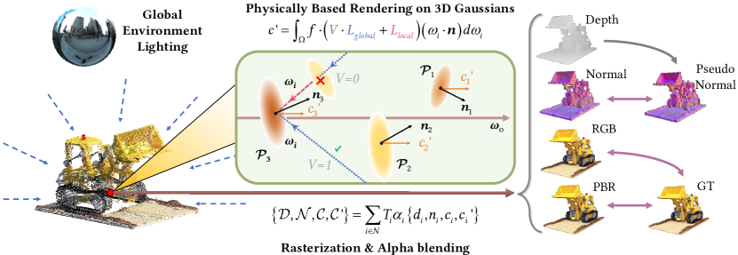
Figure 2: The proposed differentiable rendering pipeline. Starting with a collection of 3D Gaussians that embody geometry, material, and lighting attributes, we first execute the rendering equation at Gaussian level to determine the outgoing radiance of a designated viewpoint, denoted as $\boldsymbol{c^{\prime}}$. Following this, we proceed to render the corresponding features by employing rasterization coupled with alpha blending, thereby producing the vanilla color map $\mathcal{C}$, the physically based rendered color map $\mathcal{C^{\prime}}$, the depth map $\mathcal{D}$, the normal map $\mathcal{N}$, etc. To optimize relightable 3D Gaussians, we utilize the ground truth image $\mathcal{C}_{gt}$ and the pseudo normal map derived from $\mathcal{D}$ for supervision.

3 Relightable 3D Gaussians

In this section, we introduce a novel pipeline tailored for decomposing material and lighting from a collection of multi-view images based on 3DGS [22]. An overview of our pipeline is shown in Fig. 2.

3.1 Preliminaries

3D Gaussian Splatting

Distinct from the widely adopted Neural Radiance Field, 3DGS [22] employs explicit 3D Gaussian points as its primary rendering entities. A 3D Gaussian point is mathematically defined as:

$$G(\boldsymbol{x})=exp(-\frac{1}{2}(\boldsymbol{x}-\boldsymbol{\mu})^{\top}\Sigma^{-1}(\boldsymbol{x}-\boldsymbol{\mu})),$$ (1)

where $\boldsymbol{\mu}$ and $\Sigma$ denote spatial mean and covariance matrix respectively. Each Gaussian is also equipped with an opacity $o$ and a view-dependent color $\boldsymbol{c}$.

In the rendering process from a specific viewpoint, 3D Gaussians are projected onto the image plane, resulting in 2D Gaussians. The means of these 2D Gaussians are ascertained through the application of the projection matrix, the 2D covariance matrices are approximated as: $\Sigma^{\prime}=\boldsymbol{J}\boldsymbol{W}\Sigma\boldsymbol{W}^{\top}\boldsymbol{J}^{\top}$, where $\boldsymbol{W}$ and $\boldsymbol{J}$ denote the viewing transformation and the Jacobian of the affine approximation of perspective projection transformation [53]. Subsequent to this, the pixel color is derived by alpha-blending $N$ sequentially layered 2D Gaussians from front to back:

$$\mathcal{C}=\sum_{i\in{N}}T_{i}\alpha_{i}\boldsymbol{c}_{i}\text{ with }\hskip 5.0ptT_{i}=\prod_{j=1}^{i-1}(1-\alpha_{j}).$$ (2)

Here, $\alpha$ is obtained by multiplying the opacity $o$ with the 2D covariance’s contribution computed from $\Sigma^{\prime}$ and pixel coordinate in image space [22]. To maintain its meaningful interpretation throughout optimization, the covariance matrix $\Sigma$ is parameterized as a unit quaternion $\boldsymbol{q}$ and a 3D scaling vector $\boldsymbol{s}$. In summation, within the 3DGS framework, a 3D scene is represented by a set of 3D Gaussians, with the $i^{th}$ Gaussian $\mathcal{P}_{i}$ parameterized as $\{\boldsymbol{\mu}_{i},\boldsymbol{q}_{i},\boldsymbol{s}_{i},o_{i},\boldsymbol{c}_{i}\}$.

Neural Incident Light Field

NeILF [42] models the incoming lights through a neural incident light field, represented by an MLP $\mathbb{L}:\{\boldsymbol{x},\boldsymbol{\omega}_{i}\}\rightarrow L$. The MLP translates a spatial location $\boldsymbol{x}$ and an incident direction $\boldsymbol{\omega_{i}}$ into a corresponding incident light. Unlike traditional environment map, the incident light field representation exhibits spatial variability and, theoretically, possesses the capacity to proficiently model both direct and indirect lighting, as well as occlusions, within any static scene.

3.2 Geometry Enhancement

Scene geometry, specifically surface normal, is essential for realistic physically based rendering. Thus, we further regularize the scene geometry for robust BRDF estimation.

Normal Estimation

In this work, we incorporate a normal attribute $\boldsymbol{n}$ for each 3D Gaussian and devise a strategy to optimize it for PBR, which will be discussed in Sec. 3.3.

A potential methodology involves treating the spatial means of 3D Gaussians as a conventional point cloud and executing normal estimation based on the local planar assumption. However, this approach is hindered by the often sparse density of the points and, more critically, their soft nature, signifying a non-precise alignment with the object surface, which can lead to an inaccurate estimate.

To address these limitations, we propose an optimization of $\boldsymbol{n}$ from initial random vectors via back-propagation. This process entails rendering the depth and normal map for a specified viewpoint:

$$\{\mathcal{D},\mathcal{N}\}=\sum_{i\in{N}}T_{i}\alpha_{i}\{d_{i},\boldsymbol{n}_{i}\},$$ (3)

where, $d_{i}$ and $\boldsymbol{n}_{i}$ denote the depth and normal of the point. We then encourage the consistency between the rendered normal $N$ and the pseudo normal $\tilde{\mathcal{N}}$, computed from the rendered depth $\mathcal{D}$ under the local planarity assumption. The normal consistency is quantified as follows:

$$\mathcal{L}_{n}=\|\mathcal{N}-\tilde{\mathcal{N}}\|_{2}.$$ (4)

Multi-View Stereo as Geometry Clues

Real-world scenes frequently exhibit intricate geometries, posing a significant challenge for 3DGS to yield satisfactory geometry, primarily due to the prevalent geometry-appearance ambiguity [48]. To address this challenge , we propose to integrate Multi-View Stereo (MVS) geometry cues [41], which have exhibited robust performance and generalizability. We utilize Vis-MVSNet [46] to estimate per-view depth map, which is then filtered by photometric and geometric consistency checks. We strive to ensure consistency between the rendered depth $\mathcal{D}$ and the filtered MVS depth map $\mathcal{D}_{mvs}$.

$$\mathcal{L}_{d}=\|\mathcal{D}-\mathcal{D}_{mvs}\|_{1}.$$ (5)

Similar to Eq. 4 , a normal consistency $\mathcal{L}_{n,mvs}$ is also applied between the rendered normal $\mathcal{N}$ and the normal $\tilde{\mathcal{N}}_{mvs}$ calculated from the MVS depth $D_{mvs}$.

3.3 BRDF and Light Modeling

Recap on the Rendering Equation

The rendering equation [20] models light interaction with surfaces, accounting for their material properties and geometry. It is given by:

$$L_{o}(\boldsymbol{\omega_{o}},\boldsymbol{x})=\int_{\Omega}f(\boldsymbol{\omega_{o}},\boldsymbol{\omega_{i}},\boldsymbol{x})L_{i}(\boldsymbol{\omega_{i}},\boldsymbol{x})(\boldsymbol{\omega_{i}}\cdot\boldsymbol{n})d\boldsymbol{\omega_{i}},$$ (6)

where $\boldsymbol{x}$ and $\boldsymbol{n}$ are the surface point and its normal vector. $f$ models the BRDF properties, and $L_{i}$ and $L_{o}$ denote the incoming and outgoing light radiance in directions $\boldsymbol{\omega_{i}}$ and $\boldsymbol{\omega_{o}}$. $\Omega$ signifies the hemispherical domain above the surface.

Prior methods [49, 47] typically adopt a sequential pipeline that begins with the acquisition of intersection points between rays and surface through differentiable rendering and then the rendering equation is applied at these points to facilitate PBR. However, this approach presents significant challenges in the context of our framework. Although it is feasible to extract surface from the rendered depth map, querying coordinate-based global neural fields at these surface points imposes an excessive computational cost as the rendering equation needs to be applied to millions of surface points to render the whole image in each iteration. To address this problem, We propose to compute PBR color $\{c_{i}^{\prime}\}_{i=0}^{N}$ at Gaussian level first, followed by rendering the PBR image $C^{\prime}$ through alpha-blending (Fig. 2): $\mathcal{C^{\prime}}=\sum_{i\in{N}}T_{i}\alpha_{i}\boldsymbol{c}_{i}^{\prime}$. This method is more efficient for two main reasons. First, PBR is performed on fewer 3D Gaussians rather than every pixel, as each Gaussian affects multiple pixels based on its scale. Second, by allocating discrete attributes for each Gaussian, we avoid the need for global neural fields.

BRDF Parameterization

As stated above, We assign additional BRDF properties to each Gaussian: a base color $\boldsymbol{b}\in[0,1]^{3}$, a roughness $r\in[0,1]$ and a metallic $m\in[0,1]$. We adopt the simplified Disney BRDF model as in  [42]. The BRDF function $f$ in Eq. 6 is divided into a diffuse term $f_{d}=\frac{1-m}{\pi}\cdot\boldsymbol{b}$ and a specular term:

$$f_{s}(\boldsymbol{\omega}_{o},\boldsymbol{\omega}_{i})=\frac{D(\boldsymbol{h};r)\cdot F(\boldsymbol{\omega}_{o},\boldsymbol{h};\boldsymbol{b},m)\cdot G(\boldsymbol{\omega}_{i},\boldsymbol{\omega}_{o},h;r)}{(\boldsymbol{n}\cdot\boldsymbol{\omega}_{i})\cdot(\boldsymbol{n}\cdot\boldsymbol{\omega}_{o})},$$ (7)

where $\boldsymbol{h}$ is the half vector, D, F and G represent the normal distribution function, Fresnel term and geometry term.

Incident Light Modeling

Optimizing a NeILF for each Gaussian directly can be overly unconstrained, making it difficult to accurately decompose incident light from its appearance. We apply a prior by dividing the incident light into global and local components. The sampled incident light at a Gaussian from direction $\boldsymbol{\omega}_{i}$ is represented as:

$$L_{i}(\boldsymbol{\omega}_{i})=V(\boldsymbol{\omega}_{i})\cdot L_{global}(\boldsymbol{\omega}_{i})+L_{local}(\boldsymbol{\omega}_{i}),$$ (8)

where the visibility term $V(\boldsymbol{\omega}_{i})$ and the local light term $L_{local}(\boldsymbol{\omega}_{i})$ are parameterized as Spherical Harmonics (SH) for each Gaussian, denoted as $\boldsymbol{v}$ and $\boldsymbol{l}$ respectively. The global light term is parameterized as a globally shared SH, denoted as $\boldsymbol{l}^{env}$. For each 3D Gaussian, we sample $N_{s}$ incident directions over the hemisphere space through Fibonacci sampling [42] to provide numerical integration for Eq. 6. The PBR color of the Gaussian is then given by:

$$\boldsymbol{c^{\prime}(\boldsymbol{\omega}_{o})}=\sum_{i=0}^{N_{s}}(f_{d}+f_{s}(\boldsymbol{\omega}_{o},\boldsymbol{\omega}_{i}))L_{i}(\boldsymbol{\omega}_{i})(\boldsymbol{\omega}_{i}\cdot\boldsymbol{n})\Delta\boldsymbol{\omega}_{i},$$ (9)

To summarize, our method represents a 3D scene as a set of relightable 3D Gaussians and a global environment light $\boldsymbol{l}^{env}$, where the $i^{th}$ Gaussian $\mathcal{P}_{i}$ is parameterized as $\{\boldsymbol{\mu}_{i},\boldsymbol{q}_{i},\boldsymbol{s}_{i},o_{i},\boldsymbol{c}_{i},\boldsymbol{n}_{i},\boldsymbol{b}_{i},r_{i},m_{i},\boldsymbol{v}_{i},\boldsymbol{l}_{i}\}$.

3.4 Regularization

As pointed out in NeILF [42], an ambiguity exists between materials and lighting in the optimization process. To address this, regularizations are implemented to facilitate a plausible decomposition of material and lighting.

Base Color Regularization

We introduce a novel regularization for base color, according to the premise that an ideal base color should exhibit certain tonal similarities with the observed image $\mathcal{C}$ while remaining free from shadows and highlights. We generate an image $\mathcal{C}_{target}$ with reduced shadows and highlights, serving as a reference for the rendered base color $\mathcal{C}_{b}$, derived by $\mathcal{C}_{b}=\sum_{i\in{N}}T_{i}\alpha_{i}\boldsymbol{b}_{i}$:

$$\mathcal{L}_{b}=\|\mathcal{C}_{b}-\mathcal{C}_{target}\|_{1},$$ (10)

where $\mathcal{C}_{target}=w\cdot\mathcal{C}_{h}+(1-w)\cdot\mathcal{C}_{s}$. Here, $\mathcal{C}_{s}=1-(1-\mathcal{C})\cdot(1-\mathcal{C})$ and $\mathcal{C}_{h}=\mathcal{C}\cdot\mathcal{C}$ represent the shadow-reduction and highlight-reduction images, respectively and $w=1/(1+\exp(-\psi(\mathcal{C}_{v}-0.5)))$ is the weight, with $\psi$ experimentally set to 5 and $\mathcal{C}_{v}=max(R,G,B)$ is the value component of HSV color. The value component effectively distinguishes between highlights and shadows, independent of the hue of the light source, as the maximum operation closely approximates demodulation [16].

Light Regularization

We apply light regularization assuming a near-natural white incident light [26].

$$\mathcal{L}_{light}=\sum\nolimits_{c}(L_{c}-\frac{1}{3}\sum\nolimits_{c}L_{c}),c\in\{R,G,B\}.$$ (11)

Bilateral Smoothness

We expect that the BRDF properties will not change drastically in areas with smooth color [42]. We define a smooth constraint on metallic as:

$$\mathcal{L}_{s,m}=\|\nabla M\|\exp(-\|\nabla C_{gt}\|),$$ (12)

where $M$ is the rendered metallic map, given by $M=\sum_{i\in{N}}T_{i}\alpha_{i}m_{i}$. Similarly, we also define smoothness constraints $L_{s,r}$ and $L_{s,b}$ on roughness and base color.

4 Point-based Ray Tracing

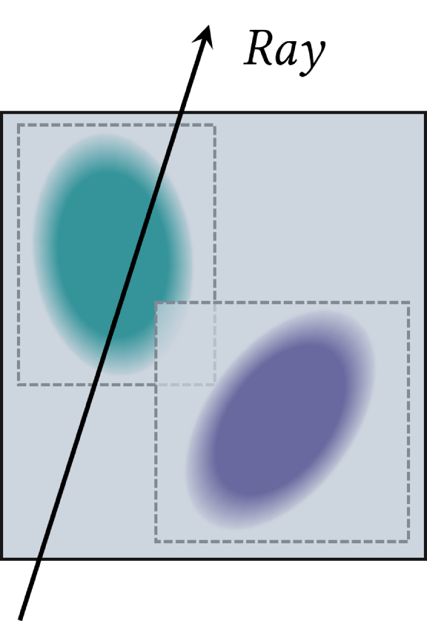
(a) Root node

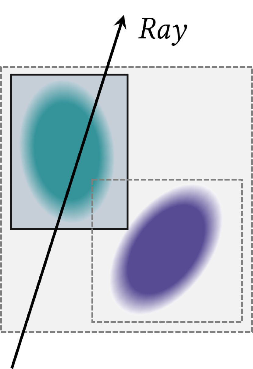
(b) Child nodes

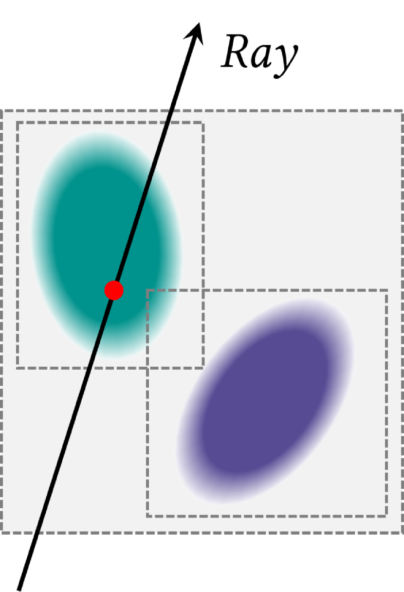
(c) Gaussian

Figure 3: Intersection point between ray and Gaussian is obtained by (a) intersects the BVH root node; (b) dive into the intersect child node recursively until the leaf node; (c) perform Eq. 13 to get the exact intersection position.

NeILF++ [48]
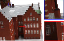
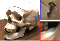
Nvdiffrec [29]
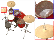
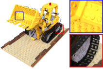
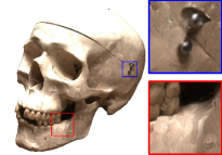
Ours
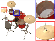
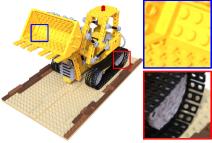
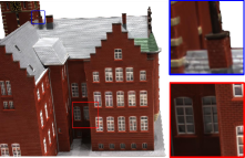
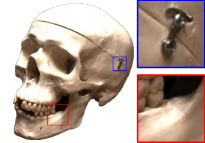
GT

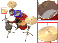
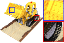
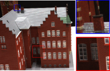
Figure 4: Qualitative results of novel view synthesis on NeRF synthetic dataset [27] and DTU dataset [19] compared with baselines.

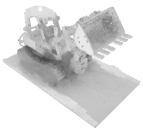
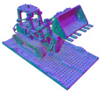
PBR	Base Color	Metallic	Roughness	Visibility	Normal

Figure 5: Qualitative results of BRDF estimation. Here we visualize the rendered average visibility (ambient occlusion) as well.

For real-time and realistic rendering with accurate shadow effects on relightable 3D Gaussians, we introduce a novel point-based ray-tracing approach in this section.

4.1 Ray Tracing on 3D Gaussians

Our proposed ray tracing technique on 3D Gaussians is built upon the Bounding Volume Hierarchy (BVH), enabling efficient querying of visibility along a ray. Our method adopts the idea from  [21], an in-place algorithm for constructing a binary radix tree that maximizes parallelism and facilitates real-time BVH construction. This capability is pivotal for integrating ray tracing within the training process. Specifically, in each iteration, we construct a binary radix tree from 3D Gaussians, where each leaf node represents the tight bounding box of a Gaussian, and each internal node denotes the bounding box of its two children.

Unlike ray tracing with opaque polygonal meshes, where only the closest intersection point is required, ray tracing with semi-transparent Gaussians necessitates accounting for all Gaussians potentially influencing the ray’s transmittance. In 3DGS, a Gaussian’s contribution to a pixel is calculated in 2D pixel space. As discussed in Sec. 3.1, transforming a 3D Gaussian to a 2D Gaussian involves an approximation, complicating the identification of an equivalent 3D point with the same influence as a 2D Gaussian in pixel space. Drawing inspiration from [23], we approximate the position of this influential 3D point along the ray where the 3D Gaussian’s contribution peaks:

$$t_{j}=\frac{(\boldsymbol{\mu}-\boldsymbol{r_{o}})^{T}\boldsymbol{\Sigma}\boldsymbol{r_{d}}}{\boldsymbol{r_{d}}^{T}\boldsymbol{\Sigma}\boldsymbol{r_{d}}},$$ (13)

where $\boldsymbol{r_{o}}$ and $\boldsymbol{r_{d}}$ denote the ray’s origin and direction vector, corresponding to the previously mentioned $\boldsymbol{\omega}_{i}$. Subsequently, we can determine $\alpha_{j}$, representing the contribution of a Gaussian to the ray, as: $\alpha_{j}=o_{i}G(\boldsymbol{r_{o}}+t_{j}\boldsymbol{r_{d}})$.

Considering the equation for transmittance along a ray: $T_{i}=\prod_{j=1}^{i-1}(1-\alpha_{j})$, it is evident that the order of $\alpha_{j}$ does not affect $T_{i}$, indicating that the order in which Gaussians are encountered along a ray does not impact the overall transmittance. As illustrated in Fig. 3, starting from the root node of the binary radix tree, intersection tests are recursively performed between the ray and the bounding volumes of each node’s children. Upon reaching a leaf node, the associated Gaussian is identified. Through this traversal, the transmittance $T$ is progressively attenuated:

$$T_{i}=(1-\alpha_{i-1})T_{i-1},\quad\text{for }i=1,\ldots,j-1\text{ with }T_{1}=1.$$ (14)

To speed up ray tracing, the process is terminated if a ray’s transmittance drops below a certain threshold $T_{min}$.

4.2 Visibility Estimation and Baking

In Sec. 3.3, we have identified a potential ambiguity in the decomposition of local and global light. The critical visibility term $V$ for reasonable decomposition can be derived by our proposed ray tracing. However, due to the computational complexity, directly querying the visibility term in Eq. 8 via ray tracing during the optimization is not preferred. Instead, based on the observation that the visibility of a single ray depends solely on the geometry of 3D Gaussians, we first bake the visibility of a ray into the 3D Gaussians by integrating the $\alpha_{i}$ from corresponding Gaussians along its path and then supervise the trainable visibility with the traced visibility $T$:

$$\mathcal{L}_{v}=\|V-T\|_{2}.$$ (15)

Due to the visibility baking, the supervision does not impose much of a burden as it requires a significantly reduced number of random rays to perform ray tracing. Moreover, the baked visibility greatly facilitates our real-time rendering with precise shading effects.

4.3 Realistic Relighting

We formulate an exhaustive graphics pipeline tailored for our relightable 3D Gaussians. This pipeline demonstrates adaptability across diverse scenes, enabling seamless relighting operations under varied environmental maps. When combining multiple objects, each represented by a set of relightable 3D Gaussians, into a new scene under a distinct environment map, our pipeline initiates by fine-tuning the baked visibility term $v$ for each Gaussian point through ray tracing (Sec. 4.1) to accurately update occlusion correlations between the objects. Subsequently, the rendering process unfolds according to our methodology (Sec. 3.3), beginning with the application of PBR at the Gaussian level and concluding with the utilization of alpha blending. Through the aforementioned approach, we can render an image efficiently with accurate shadow effects. Furthermore, in the context of offline rendering, relying solely on our ray tracing for 3D Gaussians, we can achieve a even superior image quality. A rendering from our point-based graphics pipeline, vividly showcasing highly realistic shadow effects, is prominently depicted in Fig. 1.

5 Experiments

5.1 Training Details

Table 1: Losses $\{\mathcal{L}_{i}\}$ and Weights $\{\lambda_{i}\}$. Those utilized in Stage 1 are carried over to Stage 2. ✘: Not used in synthetic data.

Stage 1	$\mathcal{L}_{i}$	$\mathcal{L}_{1}$	$\mathcal{L}_{\mathrm{ssim}}$	$\mathcal{L}_{n}$	$\mathcal{L}_{n,mvs}$	$\mathcal{L}_{d}$	$\mathcal{L}_{entropy}$
	$\lambda_{i}$	0.8	0.2	0.01	0.01✘	1✘	0.1
Stage 2	$\mathcal{L}_{i}$	$\mathcal{L}_{b}$	$\mathcal{L}_{light}$	$\mathcal{L}_{s,b}$	$\mathcal{L}_{s,r}$	$\mathcal{L}_{s,m}$	$\mathcal{L}_{v}$
	$\lambda_{i}$	0.01	0.01	6e-3	2e-3	2e-3	0.1

Table 2: Quantitative results for NVS on NeRF synthetic dataset.

	Geometry	Relighting	PSNR $\uparrow$	SSIM $\uparrow$	LPIPS $\downarrow$
NPBG [1]	point	✘	28.10	0.923	0.077
NPBG++ [34]	point	✘	28.12	0.928	0.076
FreqPCR [52]	point	✘	31.24	0.950	0.049
3DGS [22]	point	✘	33.88	0.970	0.031
PhySG [49]	neural	✔	18.91	0.847	0.182
Nvdiffrec [29]	mesh	✔	29.05	0.939	0.081
NeILF++ [47]	neural	✔	26.37	0.911	0.091
Ours	point	✔	31.63	0.960	0.043

Table 3: Quantitative results on real-world DTU dataset. Our method excels in NVS quality compared to prior inverse PBR methods.

DTU Scan	24	37	40	55	63	65	69	83	97	105	106	110	114	118	122	Mean
NerFactor [51]	23.24	21.91	23.33	26.86	22.70	24.71	27.59	22.56	20.45	25.08	26.30	25.14	21.35	26.44	26.53	24.28
PhySG [49]	17.38	15.11	20.65	18.71	18.89	18.47	18.08	21.98	17.31	20.67	18.75	17.55	21.20	18.78	23.16	19.11
Neual-PIL [9]	20.67	19.51	19.12	21.01	23.70	18.94	17.05	20.54	19.88	19.67	18.20	17.75	21.38	21.69	—	19.94
Nvdiffrec [29]	18.86	20.90	20.82	19.46	25.70	22.82	20.34	25.17	20.16	24.21	20.01	21.56	20.85	22.81	25.02	21.91
NeILF++ [47]	27.31	26.21	28.19	30.07	27.47	26.79	30.92	24.63	24.56	29.25	31.58	30.69	26.93	31.33	33.19	28.61
Ours	27.87	24.98	27.31	32.02	30.89	31.22	29.45	31.88	27.05	29.63	34.36	32.94	30.54	36.76	37.31	30.95

To ensure stable optimization, the training procedure is divided into two stages. Firstly, we optimize an 3DGS [22] model, augmented with an additional normal vector $\boldsymbol{n}$ (Sec. 3.2). We also add normal gradient condition for adaptive density control. Subsequently, with the already stable geometry from the first stage, we begin with the ray tracing method (Sec. 4.1) to bake the visibility term $\boldsymbol{v}$, and then optimize the entire parameter set using the comprehensive pipeline described in Sec. 3.3. During the second stage, we sample $N_{s}=24$ rays per Gaussian for PBR. Tab. 1 provides a complete list of the used losses and their weights. We train our model for 30,000 iterations in the initial stage and 10,000 iterations in the latter. And all experiments are conducted on a single NVIDIA GeForce RTX 3090 GPU. Please see the supplementary material for more details.

Speed and Memory

To train a NeRF synthetic scene, our model typically requires approximately 16 minutes and 10 GB of memory. Notably, the visibility baking in the second stage is remarkably brief, lasting only a few seconds. Following this optimization, our model attains real-time rendering across different lighting conditions, achieving 120 frames per second.

5.2 Performance on Synthetic Data

We present the quantitative assessments for novel view synthesis (NVS) using the NeRF synthetic dataset [27]. We report three performance metrics (PSNR, SSIM, and LPIPS), averaged across all scenes, as detailed in Tab. 2. As it shows, our method demonstrates superiority over various point-based rendering techniques [1, 34, 52]. Though our performance slightly lags behind the vanilla 3DGS [22], it is noteworthy that our approach excels in the accurate estimation of object materials, presenting a notable advantage. Furthermore, in contrast to inverse rendering methods [49, 16, 47], our method showcases enhanced NVS quality, as shown in Fig. 4.

5.3 Performance on Real-World Data

Our evaluation extends to the real-world DTU dataset [19], where we emphasize again the geometric intricacies inherent in real data. Although the 3D Gaussian Splatting technique exhibits commendable rendering accuracy in real-world scenarios, it falls short in generating satisfactory geometry, thus impeding our ability to perform inverse Physically Based Rendering effectively. To circumvent this, we integrate an off-the-shelf MVS method [46] to augment the geometric fidelity of 3DGS. This enhancement, requiring merely a few minutes per scene, imposes minimal overhead. Consistent with NeILF++ [47], we selected five viewpoints per scene for evaluation. The quantitative outcomes are detailed in Tab. 3, and the qualitative results are also vividly illustrated in Fig. 4. Our method achieves superior performance in NVS and simultaneously yields credible material property estimations, as demonstrated in Fig. 5.

(a) base color wo/w light division

(b) base color wo/w $\mathcal{L}_{b}$

(c) Metallic wo/w smoothness

(d) Roughness wo/w smoothness

Figure 6: Ablation Studies on main components of our method.

5.4 Ablation Study

Ray Sample Number

First, we investigate the impact of ray sample number on the NVS quality. We sample varying numbers of incident light rays and report the average scores on NeRF synthetic dataset, as outlined in Tab. 4. Our analysis reveals that incrementing the sample number marginally enhances NVS quality, yet simultaneously escalates the computational load. Hence, to balance the dichotomy between quality and computational efficiency, a sample size of 24 was chosen.

Lighting Division

Next, we explore the influence of dividing the incident light into global and local components. In Fig. 6, we illustrate the difference between our method and optimizing the entire incident light field directly. The results indicate that light splitting facilitates a more precise estimation of incident light and yields a finer decomposition of the light components.

Regularizations

Lastly, we focus on the effectiveness of the applied regularizations. It is observed that both light regularization and the newly proposed base color regularization significantly enhance the decomposition of base color and lighting in real-world data (Fig. 6). Moreover, the application of smooth regularization proves beneficial in achieving a higher quality material estimation (Fig. 6).

Table 4: Ablation on sample number. Average scores are reported.

	PSNR $\uparrow$	SSIM $\uparrow$	LPIPS $\downarrow$	Time (min)	FPS
$N_{s}$=12	31.42	0.959	0.043	13.77	150
$N_{s}$=24	31.63	0.960	0.043	15.68	120
$N_{s}$=48	31.78	0.961	0.042	19.52	87

6 Conclusion

We have presented Relightable 3D Gaussian, a novel differentiable point-based rendering pipeline designed for scene relighting and editing. In terms of implementation, we associate each 3D Gaussian with a normal, BRDF, and incident light, optimizing them through 3DGS and inverse PBR. Our method exhibits commendable performance in Novel View Synthesis (NVS) and achieves reasonable material and light decomposition. Additionally, we introduce a ray tracing scheme tailored for scenes represented by 3D Gaussians, providing supervision for visibility and enabling realistic scene rendering. The flexibility of points and our BRDF optimization empower our pipeline to accomplish both scene relighting and editing. Notably, the rendering speed exceeds 120 FPS, attaining real-time rendering capabilities.

Limitations and Future work

Our method comes with limitations. It does not handle well for unbordered scenes and requires the presence of object masks during the optimization process. We have noticed an adverse impact from the background on our optimization process, likely due to the unique characteristics of the point clouds generated by 3D Gaussian Splatting. These point clouds resemble particles with color and some transparency, diverging from conventional surface points. Although we’ve integrated off-the-shelf Multi-View Stereo (MVS) cues for geometry enhancement, the resulting geometry still falls short of our expectations. Considering the potential benefits, exploring the integration of MVS into our optimization process for more accurate geometry stands as a promising avenue for future research.

Supplementary Material

In this supplementary document, we dive into particular aspects not comprehensively addressed in the principal manuscript due to space limitations. For the results of object compositing and relighting accomplished via our exclusive point-based rendering pipeline, we strongly recommend that readers refer to the accompanying video material provided for an enhanced understanding.

Appendix A More Implement details

A.1 Adaptive Density Control

Adaptive density control emerges as an indispensable component for the success of 3D Gaussian Splatting (3DGS) [22]. This mechanism serves a dual purpose: firstly, to eliminate points with minimal contribution, thereby reducing point redundancy; and secondly, to augment regions with suboptimal geometric reconstruction.

In the vanilla implementation of 3DGS [22], adaptive density control is executed at every $I_{d}$ iteration within the specified range from iteration $I_{start}$ to $I_{end}$. 3D Gaussians with average view-space position gradients $\Delta_{pos}$ above a threshold $\tau_{pos}$ undergo either cloning or splitting operations based on their size. However, following the native adaptive density control scheme, we find some areas where the normals fall short of satisfaction, even though the rendered image exhibits commendable quality. To address this, we introduce an additional criterion based on the normal gradient. If the accumulated average gradient of a Gaussian’s normal, denoted as $\Delta_{n}$, exceeds the threshold $\tau_{n}$, then the Gaussian is subjected to either cloning or splitting, depending on its size. The effectiveness of our added normal gradient criterion is shown in Fig. 7. Accordingly, if the normal gradient of a Gaussian, represented as $\Delta_{n}$, exceeds the threshold $\tau_{n}$, the Gaussian is then subjected to either cloning or splitting, depending on its size. The efficacy of our novel normal gradient criterion is shown in Fig 7.

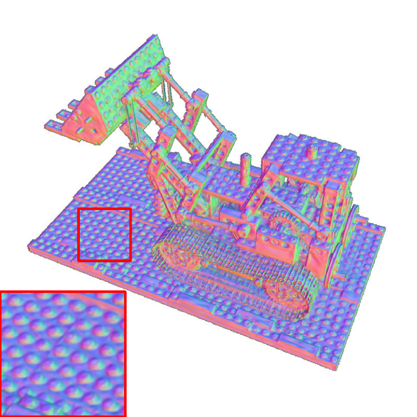
(a) with normal gradient criterion

(b) without normal gradient criterion

Figure 7: Rendered normal map with/without the normal gradient criterion on Lego from NeRF synthetic dataset [27]. The proposed normal gradient criterion for adaptive density control greatly enhance the performance of normal estimation.

Overall control over the total number of 3D Gaussian points holds paramount importance due to its direct association with both training and rendering time. We find that the total number of points can be effectively controlled without compromising the quality of Novel View Synthesis (NVS) by decreasing the frequency of densification. As the interval $I_{d}$ grows, the trends of the NVS quality (described in PSNR), number of 3D Gaussians and training time are illustrated in Fig. 8. The hyperparameters and their corresponding settings in the adaptive density control process are detailed in Tab. 5.

Table 5: Hyperparameters in Adaptive Density Control.

Hyperparameter	$I_{d}$	$I_{start}$	$I_{end}$	$\tau_{pos}$	$\tau_{n}$
Values	500	500	10,000	2e-4	4e-6

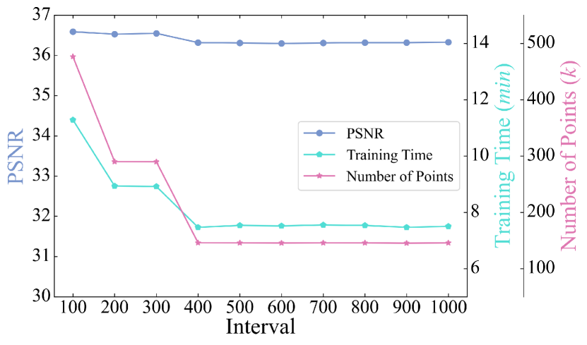
Figure 8: Trends in the quality of the novel view synthesis (described in PSNR), the overall number of Gaussian points, and the time required for optimization as the interval $I_{d}$ increases.By increasing the $I_{d}$ appropriately, the number of points can be effectively controlled, thus reducing time consumption without significant loss of accuracy.

A.2 MVS cues

For each individual view involved in the training process, we initiate by selecting the most suitable source images based on the Structure from Motion (SfM) [37, 38] results. Subsequently, we perform per-view depth estimation using Vis-MVSNet [46]. After that, photometric and multi-view geometric consistency are executed to identify and filter out inaccuracies in depth estimation. For a more comprehensive understanding of the MVS inference process, readers are referred to the detailed methodology outlined in Vis-MVSNet [46].

We observe marginal improvement from Multi-View Stereo (MVS) cues in the NeRF synthetic dataset. However, for the DTU dataset, MVS cues significantly contribute to enhanced performance. We infer that this is due to the increased complexity of geometries and lighting conditions in real-world DTU scenes, posing challenges for achieving satisfactory geometric results with the vanilla 3DGS. On the DTU data [19], the filtered MVS depth map is depicted in Fig. 9(a), while the normal map derived from it according to Eq. 16 is illustrated in Fig. 9(b). Fig. 9(c) showcases the depth map rendered, demonstrating a higher level of completeness compared to the filtered MVS depth map. Fig. 9(d), 9(e), 9(f) present the rendered normal maps when the training is regularized with $\mathcal{L}_{n}$, $\{\mathcal{L}_{n},\mathcal{L}_{n,mvs}\}$, and $\{\mathcal{L}_{n},{\mathcal{L}_{n,mvs}},\mathcal{L}_{d}\}$, respectively.

$$\tilde{\mathcal{N}}_{u,v}=\frac{\nabla_{u}{\boldsymbol{P}}\times\nabla_{v}{\boldsymbol{P}}}{\|\nabla_{u}{\boldsymbol{P}}\times\nabla_{v}{\boldsymbol{P}}\|},$$ (16)

where $(u,v)$ denotes the pixel coordinates in the image space, and $\nabla{\boldsymbol{P}}$ signifies the spatial gradient of the unprojected points derived from the rendered depth $\mathcal{D}$.

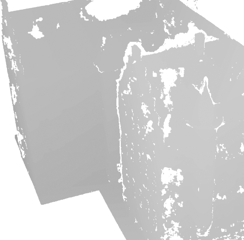
(a) MVS depth

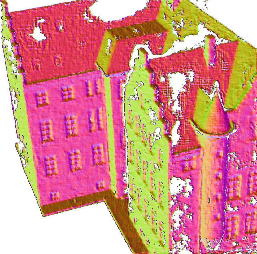
(b) MVS normal

(c) rendered depth

(d) with $\mathcal{L}_{n}$

(e) with $\{\mathcal{L}_{n},\mathcal{L}_{n,mvs}\}$

(f) with $\{\mathcal{L}_{n},\mathcal{L}_{n,mvs},\mathcal{L}_{d}\}$

Figure 9: Using MVS cues to enhance the geometric performance of 3DGS on DTU data. (a) The filtered MVS depth map, (b) the normal map derived from MVS depth, (c) the rendered depth map, (d) the rendered normal map with $\mathcal{L}_{n}$, (e) the rendered normal map with $\{\mathcal{L}_{n},\mathcal{L}_{n,mvs}\}$, (f) the rendered normal map with $\{\mathcal{L}_{n},{\mathcal{L}_{n,mvs}},\mathcal{L}_{d}\}$.

A.3 Details for Simplified BRDF

In this section, we describe the detailed implementations of the specular term in our applied BRDF model, incorporating the normal distribution term $D$, the Fresnel term $F$, and the geometry term $G$. To evaluate the normal distribution function $D$, a Spherical Gaussian function is used as follows:

$$\begin{split}D(\boldsymbol{h};r)&=S(\boldsymbol{h},\frac{1}{{\pi}r^{2}},\boldsymbol{n},\frac{2}{r^{2}})\\ &=\frac{1}{{\pi}r^{2}}\exp{\frac{2}{r^{2}}(\boldsymbol{h}\cdot\boldsymbol{n}-1)}\end{split}$$ (17)

The Fresnel term is defined as:

$$F(\boldsymbol{\omega}_{o}2,\boldsymbol{h};\boldsymbol{b},m)=F_{0}+(1-F_{0})(1-(\boldsymbol{\omega}_{o}\cdot\boldsymbol{h})^{5})$$ (18)

where, $F_{0}=0.04(1-m)+m\boldsymbol{b}$. The geometry term $G$ is approximated using two GGX function [40]:

$$G(\boldsymbol{\omega}_{i},\boldsymbol{\omega}_{o},\boldsymbol{n};r)=G_{GGX}(\boldsymbol{\omega}_{i}\cdot\boldsymbol{n})G_{GGX}(\boldsymbol{\omega}_{o}\cdot\boldsymbol{n})$$ (19)

where the GGX function is defined as

$$G_{GGX}(z)=\frac{2z}{z+\sqrt{r^{2}+(1-r^{2})z^{2}}}$$ (20)

.

A.4 Losses and Regularizations

We now provide a more detailed explanation of certain losses mentioned in the principal manuscript.

L1 Loss and SSIM loss

In the initial stage, we establish both L1 loss $\mathcal{L}_{1}$ and Structural Similarity Index (SSIM) loss $\mathcal{L}_{\mathrm{ssim}}$ metrics by comparing the rendered image $\mathcal{C}$ with the observed image $\mathcal{C}_{gt}$. Subsequently, in the second stage, L1 and SSIM are also applied to the physically based rendered image $\mathcal{C}^{\prime}$ and the observed image $\mathcal{C}_{gt}$.

Mask Entropy

We apply mask cross-entropy to mitigate the presence of unwarranted 3D Gaussians in the background region, which is defined as:

$$\begin{split}\mathcal{L}_{entropy}=-O^{m}\log{O}-(1-O^{m})\log{(1-O)},\end{split}$$ (21)

where $O^{m}$ denotes the object mask and $O$ denotes the accumulated transmittance $O=\sum_{i\in{N}}T_{i}\alpha_{i}$.

Base Color Regularization

The base color regularization is built on the observation that the base color should exhibit some tone similarity to the observed image while remaining devoid of shadows and highlights. To seek guidance, We conduct shadow and highlight reduction on the observed image $\mathcal{C}_{gt}$ and subsequently apply weighted fusion to generate an image $\mathcal{C}_{target}$ with minimal shadows and highlights. The fused image then serves as the optimization target of the base color image $\mathcal{C}_{b}$. We claim that the target image should only serve as an additional guide for the base color. Therefore, it is imperative to ensure that the weight assigned to the base color regularization is not excessively large. The base color regularization is defined as:

$$\mathcal{L}_{b}=\|C_{b}-C_{target}\|_{1}.$$ (22)

The target image is calculated by:

$$\mathcal{C}_{target}=w\cdot\mathcal{C}_{h}+(1-w)\cdot\mathcal{C}_{s}.$$ (23)

The shadow-reduction image $\mathcal{C}_{s}$ and the highlight-reduction image $\mathcal{C}_{h}$ are defined as

$$\mathcal{C}_{s}=1-(1-\mathcal{C}_{gt})\cdot(1-\mathcal{C}_{gt}),$$ (24)

and

$$\mathcal{C}_{h}={\mathcal{C}_{gt}}\cdot{\mathcal{C}_{gt}},$$ (25)

respectively. Note that the images are normalized to [0, 1].

In the shadow areas of the observed image, $\mathcal{C}_{b}$ should approximate $\mathcal{C}_{s}$, while in the highlighted areas, it should be similar to $\mathcal{C}_{h}$. The weight is defined as:

$$w=1/(1+\exp(-\psi*(V-0.5)))$$ (26)

where, the value component $V=max(R,G,B)$ of the HSV color approximates the distinction between highlights and shadows, regardless of the hue of the light source, since the maximum operation approximates the demodulation, as noted in [16]. Here, $\psi$ is experimentally set to 5 and the curve of $w$ is shown in Fig. 10.

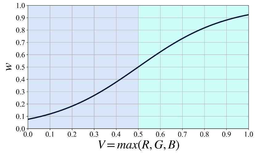
Figure 10: The curve of weight $w$ when generating the target image $\mathcal{C}_{target}$. When $V=max(R,G,B)$ is small, suggesting a higher likelihood of representing the shadow area in the observed image, and the weight $w$ is small, indicating that the target image $C_{target}$ should be more similar to the shadow-reduction image $\mathcal{C}_{s}$.

Appendix B Time for Training and Rendering

In this section, we present the training and rendering speed of various methods designed for relighting, as detailed in Tab. 6. Our method notably excels in terms of both training and rendering efficiency. Specifically, training a scene from the NeRF synthetic dataset required less than 20% of the time compared to the Mesh-based Nvdiffrec method, while maintaining comparable rendering efficiency. In comparison to the neural implicit representation based NeILF++, our method is approximately 15 and 700 times faster in training and rendering, respectively.

Table 6: Training time (time for optimization) and Rendering time (time per rendered image).

	Training Time	Rendering Time
PhySG [49]	9h	5s
Nvdiffrec []	1.5h	5ms
NeILF++ [47]	4h	14s
NerFactor [51]	days	-
Neual-PIL [9]	days	-
Ours	16min	8ms

Appendix C More Visualizations

Additional qualitative results on NeRF synthetic and DTU datasets are shown in Fig. 12.

Appendix D Composition and Relighting

We formulate an exhaustive graphics pipeline tailored for our relightable 3D Gaussians. This pipeline demonstrates adaptability across diverse scenes, enabling seamless relighting operations under varied environmental maps. After optimizing the scenes as relightable 3D Gaussians, we can effortlessly apply transformations to the scenes and composite them to generate a new scene. This capability is facilitated by the explicit discrete representation property inherent in points. Additionally, owing to our decomposition of material properties and lighting for each 3D Gaussian, our pipeline supports relighting the new scene under a distinct environment map.

Our pipeline supports both online real-time and offline high-quality rendering. In online rendering, the multi-object composition and transformations induce changes in the occlusion relationships among objects within the new scene. Consequently, the visibility ingrained in the Spherical Harmonics (SHs) of the optimized 3D Gaussians necessitates further updating to ensure accuracy in rendering. We achieve this by fine-tuning the baked visibility term $v$ for each Gaussian through ray tracing (Sec. 4.1) to accurately update occlusion correlations between the objects. Due to the efficient look-up through baked visibility $v$ and a relatively small number of sample rays (compared to offline rendering), this approach facilitates real-time rendering. In offline rendering, instead of utilizing the baked visibility, we conduct a full ray-tracing procedure on the new scene for querying more accurate visibility, which means we use the traced visibility to represent the $V(\boldsymbol{\omega}_{i})$ in Eq. 8. In Fig. 13, we demonstrate both our real-time online rendering ($N_{s}=24$) and offline high-quality rendering ($N_{s}=384$).

Apart from multi-object composition illustrated in Fig. 13, we also perform scene composition and relighting on Tanks and Temples dataset [24], which is shown in Fig. 14.

PBR
Base Color
Metallic
Roughness
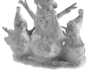
Normal

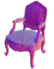
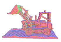
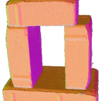
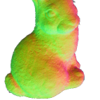
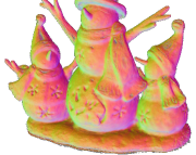
Figure 11: More qualitative results of BRDF estimation.

Visibility
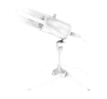
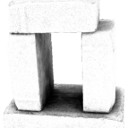
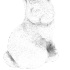
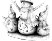
Global Lights
Local Lights
Lights

Figure 12: Qualitative results of Visibility and Lights. As in Eq. 8, Visibility denotes the average ambient occlusion $V(\boldsymbol{\omega}_{i})$, Global Light denotes the average environment light $V(\boldsymbol{\omega}_{i})L_{global}(\boldsymbol{\omega}_{i})$, Local Light denotes the average reflected light $L_{local}$, and Light denotes the average incident light $L_{i}(\boldsymbol{\omega}_{i})$.

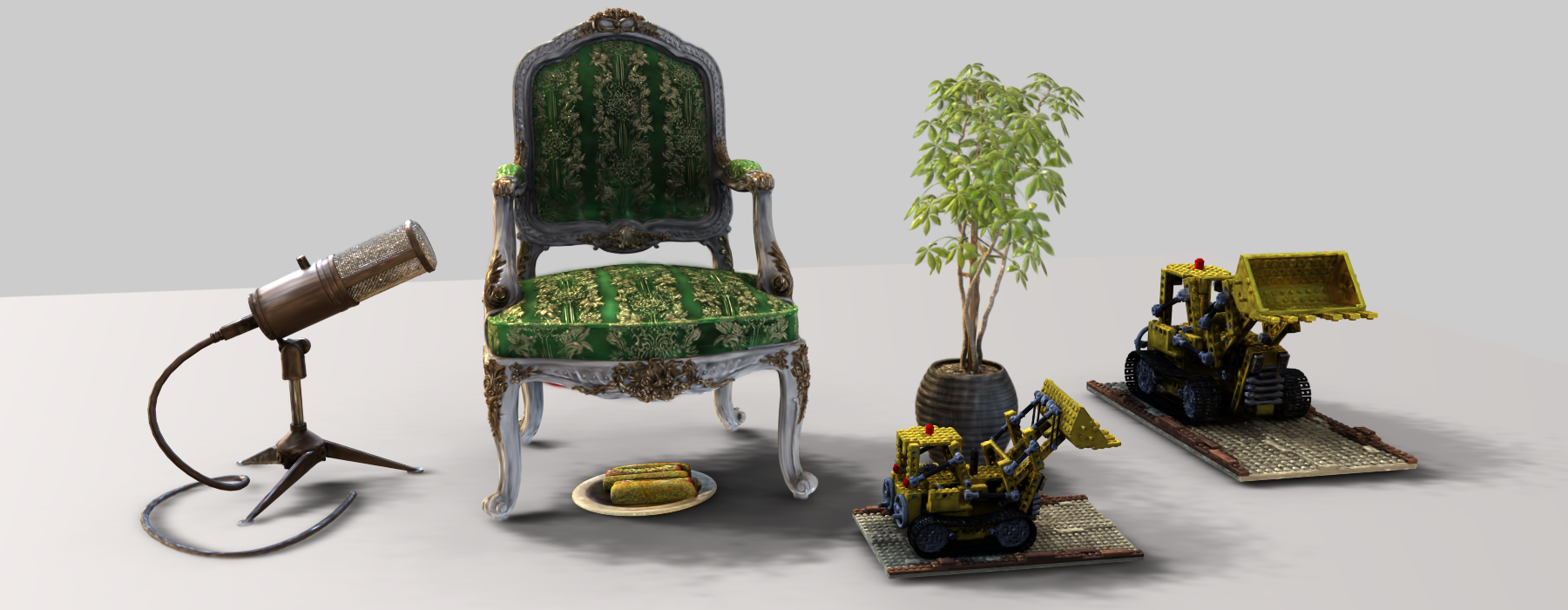
(a) Online real-time rendering (0.03 seconds).

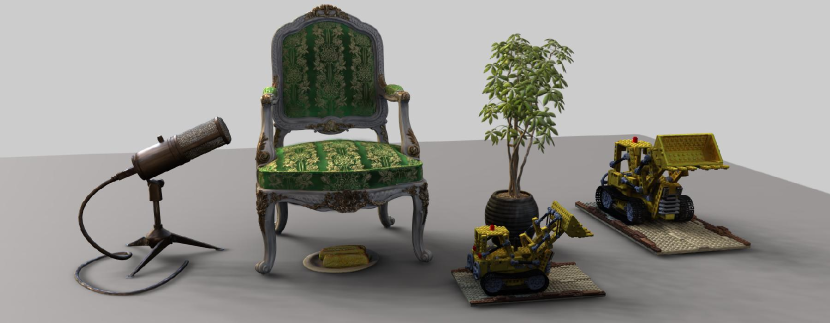
(b) Offline high-quality rendering (55 seconds).

Figure 13: Online real-time and offline high-quality rendering.

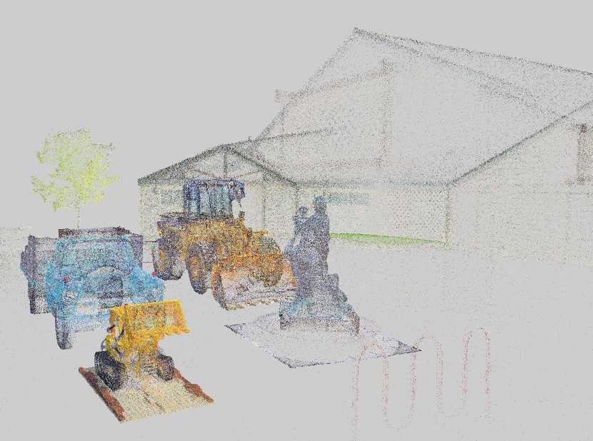
(a) Points after scene composition (colored with base color).

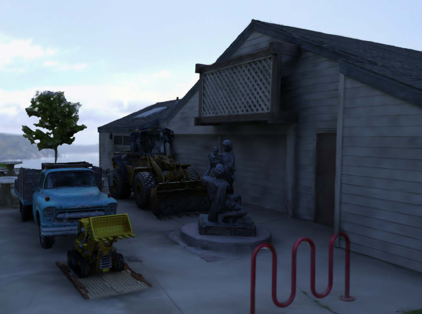
(b) Scene composition and relighting.

Figure 14: Scene composition and relighting on Tanks and Temples dataset [24].

References

- Aliev et al. [2020] Kara-Ali Aliev, Artem Sevastopolsky, Maria Kolos, Dmitry Ulyanov, and Victor Lempitsky. Neural point-based graphics. In ECCV, 2020.
- Azinovic et al. [2019] Dejan Azinovic, Tzu-Mao Li, Anton Kaplanyan, and Matthias Nießner. Inverse path tracing for joint material and lighting estimation. In CVPR, 2019.
- Barron et al. [2021] Jonathan T Barron, Ben Mildenhall, Matthew Tancik, Peter Hedman, Ricardo Martin-Brualla, and Pratul P Srinivasan. Mip-nerf: A multiscale representation for anti-aliasing neural radiance fields. In ICCV, 2021.
- Barron et al. [2022] Jonathan T Barron, Ben Mildenhall, Dor Verbin, Pratul P Srinivasan, and Peter Hedman. Mip-nerf 360: Unbounded anti-aliased neural radiance fields. In CVPR, 2022.
- Barron et al. [2023] Jonathan T Barron, Ben Mildenhall, Dor Verbin, Pratul P Srinivasan, and Peter Hedman. Zip-nerf: Anti-aliased grid-based neural radiance fields. arXiv preprint, 2023.
- Bi et al. [2020a] Sai Bi, Zexiang Xu, Pratul Srinivasan, Ben Mildenhall, Kalyan Sunkavalli, Miloš Hašan, Yannick Hold-Geoffroy, David Kriegman, and Ravi Ramamoorthi. Neural reflectance fields for appearance acquisition. arXiv preprint, 2020a.
- Bi et al. [2020b] Sai Bi, Zexiang Xu, Kalyan Sunkavalli, Miloš Hašan, Yannick Hold-Geoffroy, David Kriegman, and Ravi Ramamoorthi. Deep reflectance volumes: Relightable reconstructions from multi-view photometric images. In ECCV, 2020b.
- Bi et al. [2020c] Sai Bi, Zexiang Xu, Kalyan Sunkavalli, David Kriegman, and Ravi Ramamoorthi. Deep 3d capture: Geometry and reflectance from sparse multi-view images. In CVPR, 2020c.
- Boss et al. [2021] Mark Boss, Varun Jampani, Raphael Braun, Ce Liu, Jonathan Barron, and Hendrik Lensch. Neural-pil: Neural pre-integrated lighting for reflectance decomposition. NeurIPS, 2021.
- Chen et al. [2022] Anpei Chen, Zexiang Xu, Andreas Geiger, Jingyi Yu, and Hao Su. Tensorf: Tensorial radiance fields. In ECCV, 2022.
- Chen et al. [2023] Zhiqin Chen, Thomas Funkhouser, Peter Hedman, and Andrea Tagliasacchi. Mobilenerf: Exploiting the polygon rasterization pipeline for efficient neural field rendering on mobile architectures. In CVPR, 2023.
- Deng et al. [2022] Kangle Deng, Andrew Liu, Jun-Yan Zhu, and Deva Ramanan. Depth-supervised nerf: Fewer views and faster training for free. In CVPR, 2022.
- Fridovich-Keil et al. [2022] Sara Fridovich-Keil, Alex Yu, Matthew Tancik, Qinhong Chen, Benjamin Recht, and Angjoo Kanazawa. Plenoxels: Radiance fields without neural networks. In CVPR, 2022.
- Garbin et al. [2021] Stephan J Garbin, Marek Kowalski, Matthew Johnson, Jamie Shotton, and Julien Valentin. Fastnerf: High-fidelity neural rendering at 200fps. In ICCV, 2021.
- Guo et al. [2019] Kaiwen Guo, Peter Lincoln, Philip Davidson, Jay Busch, Xueming Yu, Matt Whalen, Geoff Harvey, Sergio Orts-Escolano, Rohit Pandey, Jason Dourgarian, et al. The relightables: Volumetric performance capture of humans with realistic relighting. ACM TOG, 2019.
- Hasselgren et al. [2022] Jon Hasselgren, Nikolai Hofmann, and Jacob Munkberg. Shape, light, and material decomposition from images using monte carlo rendering and denoising. NeurIPS, 2022.
- Hedman et al. [2021] Peter Hedman, Pratul P Srinivasan, Ben Mildenhall, Jonathan T Barron, and Paul Debevec. Baking neural radiance fields for real-time view synthesis. In ICCV, 2021.
- Hu et al. [2022] Tao Hu, Shu Liu, Yilun Chen, Tiancheng Shen, and Jiaya Jia. Efficientnerf efficient neural radiance fields. In CVPR, 2022.
- Jensen et al. [2014] Rasmus Jensen, Anders Dahl, George Vogiatzis, Engin Tola, and Henrik Aanæs. Large scale multi-view stereopsis evaluation. In CVPR, 2014.
- Kajiya [1986] James T Kajiya. The rendering equation. In Proceedings of the 13th annual conference on Computer graphics and interactive techniques, 1986.
- Karras [2012] Tero Karras. Maximizing parallelnism in the construction of bvhs, octrees, and k-d trees. In Proceedings of the Fourth ACM SIGGRAPH/Eurographics conference on High-Performance Graphics, 2012.
- Kerbl et al. [2023] Bernhard Kerbl, Georgios Kopanas, Thomas Leimkühler, and George Drettakis. 3d gaussian splatting for real-time radiance field rendering. ACM TOG, 2023.
- Keselman and Hebert [2023] Leonid Keselman and Martial Hebert. Flexible techniques for differentiable rendering with 3d gaussians. arXiv preprint, 2023.
- Knapitsch et al. [2017] Arno Knapitsch, Jaesik Park, Qian-Yi Zhou, and Vladlen Koltun. Tanks and temples: Benchmarking large-scale scene reconstruction. ACM Transactions on Graphics, 36(4), 2017.
- Levoy and Whitted [1985] Marc Levoy and Turner Whitted. The use of points as a display primitive. 1985.
- Liu et al. [2023] Yuan Liu, Peng Wang, Cheng Lin, Xiaoxiao Long, Jiepeng Wang, Lingjie Liu, Taku Komura, and Wenping Wang. Nero: Neural geometry and brdf reconstruction of reflective objects from multiview images. 2023.
- Mildenhall et al. [2020] Ben Mildenhall, Pratul P. Srinivasan, Matthew Tancik, Jonathan T. Barron, Ravi Ramamoorthi, and Ren Ng. Nerf: Representing scenes as neural radiance fields for view synthesis. In ECCV, 2020.
- Müller et al. [2022] Thomas Müller, Alex Evans, Christoph Schied, and Alexander Keller. Instant neural graphics primitives with a multiresolution hash encoding. ACM TOG, 2022.
- Munkberg et al. [2022] Jacob Munkberg, Jon Hasselgren, Tianchang Shen, Jun Gao, Wenzheng Chen, Alex Evans, Thomas Müller, and Sanja Fidler. Extracting triangular 3d models, materials, and lighting from images. In Proceedings of the IEEE/CVF Conference on Computer Vision and Pattern Recognition, pages 8280–8290, 2022.
- Nam et al. [2018] Giljoo Nam, Joo Ho Lee, Diego Gutierrez, and Min H Kim. Practical svbrdf acquisition of 3d objects with unstructured flash photography. ACM TOG, 2018.
- Park et al. [2020] Jeong Joon Park, Aleksander Holynski, and Steven M Seitz. Seeing the world in a bag of chips. In CVPR, 2020.
- Pfister et al. [2000] Hanspeter Pfister, Matthias Zwicker, Jeroen Van Baar, and Markus Gross. Surfels: Surface elements as rendering primitives. In Proceedings of the 27th annual conference on Computer graphics and interactive techniques, 2000.
- Pittaluga et al. [2019] Francesco Pittaluga, Sanjeev J Koppal, Sing Bing Kang, and Sudipta N Sinha. Revealing scenes by inverting structure from motion reconstructions. In CVPR, 2019.
- Rakhimov et al. [2022] Ruslan Rakhimov, Andrei-Timotei Ardelean, Victor Lempitsky, and Evgeny Burnaev. Npbg++: Accelerating neural point-based graphics. In CVPR, 2022.
- Reiser et al. [2021] Christian Reiser, Songyou Peng, Yiyi Liao, and Andreas Geiger. Kilonerf: Speeding up neural radiance fields with thousands of tiny mlps. In ICCV, 2021.
- Schmitt et al. [2020] Carolin Schmitt, Simon Donne, Gernot Riegler, Vladlen Koltun, and Andreas Geiger. On joint estimation of pose, geometry and svbrdf from a handheld scanner. In CVPR, 2020.
- Schönberger and Frahm [2016] Johannes Lutz Schönberger and Jan-Michael Frahm. Structure-from-motion revisited. In CVPR, 2016.
- Schönberger et al. [2016] Johannes Lutz Schönberger, Enliang Zheng, Marc Pollefeys, and Jan-Michael Frahm. Pixelwise view selection for unstructured multi-view stereo. In ECCV, 2016.
- Srinivasan et al. [2021] Pratul P Srinivasan, Boyang Deng, Xiuming Zhang, Matthew Tancik, Ben Mildenhall, and Jonathan T Barron. Nerv: Neural reflectance and visibility fields for relighting and view synthesis. In CVPR, 2021.
- Walter et al. [2007] Bruce Walter, Stephen R Marschner, Hongsong Li, and Kenneth E Torrance. Microfacet models for refraction through rough surfaces. In Proceedings of the 18th Eurographics conference on Rendering Techniques, pages 195–206, 2007.
- Yao et al. [2018] Yao Yao, Zixin Luo, Shiwei Li, Tian Fang, and Long Quan. Mvsnet: Depth inference for unstructured multi-view stereo. In ECCV, 2018.
- Yao et al. [2022] Yao Yao, Jingyang Zhang, Jingbo Liu, Yihang Qu, Tian Fang, David McKinnon, Yanghai Tsin, and Long Quan. Neilf: Neural incident light field for physically-based material estimation. In ECCV, 2022.
- Yariv et al. [2021] Lior Yariv, Jiatao Gu, Yoni Kasten, and Yaron Lipman. Volume rendering of neural implicit surfaces. NeurIPS, 2021.
- Yifan et al. [2019] Wang Yifan, Felice Serena, Shihao Wu, Cengiz Öztireli, and Olga Sorkine-Hornung. Differentiable surface splatting for point-based geometry processing. ACM TOG, 2019.
- Yu et al. [2022] Zehao Yu, Songyou Peng, Michael Niemeyer, Torsten Sattler, and Andreas Geiger. Monosdf: Exploring monocular geometric cues for neural implicit surface reconstruction. NeurIPS, 2022.
- Zhang et al. [2023a] Jingyang Zhang, Shiwei Li, Zixin Luo, Tian Fang, and Yao Yao. Vis-mvsnet: Visibility-aware multi-view stereo network. IJCV, 2023a.
- Zhang et al. [2023b] Jingyang Zhang, Yao Yao, Shiwei Li, Jingbo Liu, Tian Fang, David McKinnon, Yanghai Tsin, and Long Quan. Neilf++: Inter-reflectable light fields for geometry and material estimation. In ICCV, 2023b.
- Zhang et al. [2020] Kai Zhang, Gernot Riegler, Noah Snavely, and Vladlen Koltun. Nerf++: Analyzing and improving neural radiance fields. arXiv preprint, 2020.
- Zhang et al. [2021a] Kai Zhang, Fujun Luan, Qianqian Wang, Kavita Bala, and Noah Snavely. Physg: Inverse rendering with spherical gaussians for physics-based material editing and relighting. In CVPR, 2021a.
- Zhang et al. [2022] Qiang Zhang, Seung-Hwan Baek, Szymon Rusinkiewicz, and Felix Heide. Differentiable point-based radiance fields for efficient view synthesis. In SIGGRAPH Asia 2022 Conference Papers, 2022.
- Zhang et al. [2021b] Xiuming Zhang, Pratul P Srinivasan, Boyang Deng, Paul Debevec, William T Freeman, and Jonathan T Barron. Nerfactor: Neural factorization of shape and reflectance under an unknown illumination. ACM TOG, 2021b.
- Zhang et al. [2023c] Yi Zhang, Xiaoyang Huang, Bingbing Ni, Teng Li, and Wenjun Zhang. Frequency-modulated point cloud rendering with easy editing. In CVPR, 2023c.
- Zwicker et al. [2001] Matthias Zwicker, Hanspeter Pfister, Jeroen Van Baar, and Markus Gross. Surface splatting. In Proceedings of the 28th annual conference on Computer graphics and interactive techniques, 2001.
- Zwicker et al. [2002] Matthias Zwicker, Hanspeter Pfister, Jeroen Van Baar, and Markus Gross. Ewa splatting. IEEE Transactions on Visualization and Computer Graphics, 2002.