Supplementary Material: Weakly-Supervised 3D Reconstruction of Clothed Humans via Normal Maps

Appendix A Ray-Tracing the Implicit Surface Directly

As an alternative to Marching Tetrahedra, consider casting a ray to find an intersection point with the implicit surface and subsequently using the normal vector defined (directly) by the implicit surface at that intersection point. A number of existing works consider such approaches in various ways, see e.g. [niemeyer2020differentiable, yariv2020multiview, bangaru2022differentiable, chen2022gdna, vicini2022differentiable]. Perturbations of the intersection point depend on perturbations of the $\phi$ values on the vertices of the tetrahedron that the intersection point lies within. If a change in $\phi$ values causes the intersection point to no longer be contained inside the tetrahedron, one would need to discontinuously jump to some other tetrahedron (which could be quite far away, if it even exists). A potential remedy for this would be to define a virtual implicit surface that extends out of the tetrahedron in a way that provides some sort of continuity (especially along silhouette boundaries).

Comparatively, our Marching Tetrahedra approach allows us to presume (for example) that the point of intersection remains fixed on the face of the triangle even as the triangle moves. Since the implicit surface has no explicit parameterization, one is unable to similarly hold the intersection point fixed. The implicit surface utilizes an Eulerian point of view where the rays (which represent the discretization) are held fixed while the implicit surface moves (as $\phi$ values change), in contrast to our Lagrangian discretization where the rays are allowed to move/bend in order to follow fixed intersection points during differentiation. A similar approach for an implicit surface would hold the intersection point inside the tetrahedron fixed even as $\phi$ changes. Although such an approach holds potential due to the fact that implicit surfaces are amenable to computing derivatives off of the surface itself, the merging/pinching of isocontours created by convexity/concavity would likely lead to various difficulties. Furthermore, other issues would need to be addressed as well, e.g. the gradients (and thus normals) are only piecewise constant (and thus discontinuous) in the piecewise linear tetrahedral mesh basis.

Appendix B Skinning

There are two options for the algorithm ordering between skinning and Marching Tetrahedra (the latter of which reverses the order in Figure LABEL:fig:pipeline). For skinning the triangle mesh, the skinned position of each triangle mesh vertex is $v_{i}(\theta,\phi)=\sum_{j}w_{ij}(\phi)T_{j}(\theta)v_{i}^{j}(\phi)$ where $v_{i}^{j}$ is the location of $v_{i}$ in the untransformed reference space of joint $j$. Unlike in Section LABEL:sec:skinning where $w_{kj}$ and $u_{k}^{j}$ were fixed, $w_{ij}$ and $v_{i}^{j}$ both vary yielding three terms in the product rule. $\partial v_{i}^{j}/\partial\phi$ is computed according to Equation LABEL:eq:mt_grad, noting that $u_{k_{1}}$ and $u_{k_{2}}$ are fixed. $w_{ij}(\phi)$ is defined similarly to Equation LABEL:eq:zero_crossing,

$$w_{ij}=\frac{-\phi_{k_{2}}}{\phi_{k_{1}}-\phi_{k_{2}}}w_{k_{1}j}+\frac{\phi_{k_{1}}}{\phi_{k_{1}}-\phi_{k_{2}}}w_{k_{2}j}$$ (1)

where $w_{k_{1}j}$ and $w_{k_{2}j}$ are fixed; similar to Equation LABEL:eq:mt_grad, $\partial w_{ij}/\partial\phi$ will contain $\mathcal{O}(1/\epsilon)$ coefficients. For skinning the tetrahedral mesh, Equations LABEL:eq:zero_crossing and LABEL:eq:mt_grad directly define $v_{i}$ and $\partial v_{i}/\partial\phi$ since the skinning is moved to the tetrahedral mesh vertices $u_{k}$. Then, $\partial v_{i}/\partial u_{k}$ is computed according to Equation LABEL:eq:zero_crossing in order to chain rule to skinning (i.e. to $\partial u_{k}/\partial\theta$, which is computed according to the equations in Section LABEL:sec:skinning).

Appendix C Image Rasterization Implementation

C.1 Normals

Recall (from Section LABEL:sec:mt) that triangle vertices are reordered (if necessary) in order to obtain outward-pointing face normals. The area-weighted outward face normal is

$$n_{f}(v_{1},v_{2},v_{3})=\frac{1}{2}(v_{2}-v_{1})\times(v_{3}-v_{1})$$ (2)

where

$$Area(v_{1},v_{2},v_{3})=\frac{1}{2}||(v_{2}-v_{1})\times(v_{3}-v_{1})||_{2}$$ (3)

is the area weighting. Area-averaged vertex unit normals $\hat{n}_{v}$ are computed via

$$\begin{split}n_{v}=\sum_{f}n_{f}\quad\quad\quad\quad\hat{n}_{v}&=\frac{n_{v}}{||n_{v}||_{2}}\end{split}$$ (4)

where $f$ ranges over all the triangle faces that include vertex $v$. Note that one can drop the 1/2 in Equation 2, since it cancels out when computing $\hat{n}_{v}$ in Equation 4.

C.2 Camera Model

The camera rotation and translation are used to transform each vertex $v_{g}$ of the geometry to the camera view coordinate system (where the origin is located at the camera aperture), i.e. $v_{c}=Rv_{g}+T$. The normalized device coordinate system normalizes geometry in the viewing frustum (with $z\in[n,f]$) so that all $x,y\in[-1,1]$ and all $z\in[0,1]$. See Figure 1, left. Vertices are transformed into this coordinate system via

$$\begin{split}\begin{bmatrix}[v_{NDC}]\hskip 2.84526ptz_{c}\\ z_{c}\end{bmatrix}&=\begin{bmatrix}\frac{2n}{W}&0&0&0\\ 0&\frac{2n}{H}&0&0\\ 0&0&\frac{f}{f-n}&\frac{-fn}{f-n}\\ 0&0&1&0\end{bmatrix}\begin{bmatrix}[v_{c}]\\ 1\end{bmatrix}\end{split}$$ (5)

where $H=2n\tan(\theta_{\text{fov}}/2)$ is the height of the image, $\theta_{\text{fov}}$ is the field of view, $W=Ha$ is the width of the image, and $a$ is the aspect ratio. The screen coordinate system is obtained by transforming the origin to the top left corner of the image, with $+x$ pointing right and $+y$ pointing down. See Figure 1, right. Vertices are transformed into this coordinate system via

$$\begin{bmatrix}[v^{\prime}]\\ 1\end{bmatrix}=\begin{bmatrix}-W/2&0&0&W/2\\ 0&-H/2&0&H/2\\ 0&0&1&0\\ 0&0&0&1\\ \end{bmatrix}\begin{bmatrix}[v_{NDC}]\\ 1\end{bmatrix}$$ (6)

or via

$$\begin{split}\begin{bmatrix}[v^{\prime}]\hskip 2.84526ptz_{c}\\ z_{c}\end{bmatrix}&=\begin{bmatrix}-n&0&W/2&0\\ 0&-n&H/2&0\\ 0&0&\frac{f}{f-n}&\frac{-fn}{f-n}\\ 0&0&1&0\\ \end{bmatrix}\begin{bmatrix}[v_{c}]\\ 1\end{bmatrix}\\ \end{split}$$ (7)

which is obtained by multiplying both sides of Equation 6 by $z_{c}$ and substituting in Equation 5.

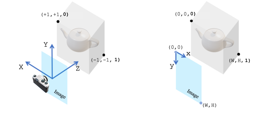
Figure 1: The normalized device (left) and screen (right) coordinate systems used during rasterization (based on Pytorch3D conventions).

C.3 Normal Map

For each pixel, a ray is cast from the camera aperture through the pixel center to find its first intersection with the triangulated surface at a point $p$ in world space. Denoting $v_{1},v_{2},v_{3}$ as the vertices of the intersected triangle, barycentric weights for the intersection point

$$\begin{split}\hat{\alpha}_{1}&=\frac{Area(p,v_{2},v_{3})}{Area(v_{1},v_{2},v_{3})}\\ \hat{\alpha}_{2}&=\frac{Area(v_{1},p,v_{3})}{Area(v_{1},v_{2},v_{3})}\\ \hat{\alpha}_{3}&=\frac{Area(v_{1},v_{2},p)}{Area(v_{1},v_{2},v_{3})}\end{split}$$ (8)

are used to compute a rotated (into screen space) unit normal from the unrotated vertex unit normals (see Equation 4) via

$$\hat{n}=R\frac{\hat{\alpha}_{1}\hat{n}_{v_{1}}+\hat{\alpha}_{2}\hat{n}_{v_{2}}+\hat{\alpha}_{3}\hat{n}_{v_{3}}}{||\hat{\alpha}_{1}\hat{n}_{v_{1}}+\hat{\alpha}_{2}\hat{n}_{v_{2}}+\hat{\alpha}_{3}\hat{n}_{v_{3}}||}$$ (9)

for the normal map. Note that dropping the denominators in Equation 8 does not change $\hat{n}$.

C.4 Scanline Rendering

After projecting a visible triangle into the screen coordinate system (via Equation 7), its projected area can be computed as

$$\begin{split}Area2D(v_{1}^{\prime},v_{2}^{\prime},v_{3}^{\prime})&=-\frac{1}{2}det\begin{pmatrix}x_{2}^{\prime}-x_{1}^{\prime}&y_{2}^{\prime}-y_{1}^{\prime}\\ x_{3}^{\prime}-x_{1}^{\prime}&y_{3}^{\prime}-y_{1}^{\prime}\\ \end{pmatrix}\end{split}$$ (10)

similar to Equation 3 (where the negative sign accounts for the fact that visible triangles have normals pointing towards the camera). When a projected triangle overlaps a pixel center $p^{\prime}$, barycentric weights for $p^{\prime}$ are computed by using $Area2D$ instead of $Area$ in Equation 8. Notably, un-normalized world space barycentric weights can be computed from un-normalized screen space barycentric weights via $\alpha_{1}=z_{2}^{\prime}z_{3}^{\prime}\alpha_{1}^{\prime}$, $\alpha_{2}=z_{1}^{\prime}z_{3}^{\prime}\alpha_{2}^{\prime}$, $\alpha_{3}=z_{1}^{\prime}z_{2}^{\prime}\alpha_{3}^{\prime}$ or

$$\begin{split}\alpha_{1}&=z_{2}^{\prime}z_{3}^{\prime}Area2D(p^{\prime},v_{2}^{\prime},v_{3}^{\prime})\\ \alpha_{2}&=z_{1}^{\prime}z_{3}^{\prime}Area2D(v_{1}^{\prime},p^{\prime},v_{3}^{\prime})\\ \alpha_{3}&=z_{1}^{\prime}z_{2}^{\prime}Area2D(v_{1}^{\prime},v_{2}^{\prime},p^{\prime})\end{split}$$ (11)

giving

$$\hat{n}=R\frac{\alpha_{1}\hat{n}_{v_{1}}+\alpha_{2}\hat{n}_{v_{2}}+\alpha_{3}\hat{n}_{v_{3}}}{||\alpha_{1}\hat{n}_{v_{1}}+\alpha_{2}\hat{n}_{v_{2}}+\alpha_{3}\hat{n}_{v_{3}}||}$$ (12)

as an (efficient) alternative to Equation 9. If more than one triangle overlaps $p^{\prime}$, the closest one (i.e. the one with the smallest value of $z^{\prime}=\hat{\alpha}_{1}^{\prime}z_{1}^{\prime}+\hat{\alpha}_{2}^{\prime}z_{2}^{\prime}+\hat{\alpha}_{3}^{\prime}z_{3}^{\prime}$ at $p^{\prime}$) is chosen.

C.5 Computing Gradients

For each pixel overlapped by the triangle mesh, the derivative of the normal (in Equation 12) with respect to the vertices of the triangle mesh is required, i.e. $\partial\alpha_{i}/\partial v_{g}$ and $\partial\hat{n}_{v_{i}}/\partial v_{g}$ are required. $\partial\alpha_{i}/\partial v^{\prime}$ can be computed from Equations 11 and 10, $\partial v^{\prime}/\partial v_{c}$ can be computed from Equation 7, and $\partial v_{c}/\partial v_{g}$ can be computed from $v_{c}=Rv_{g}+T$. $\partial\hat{n}_{v_{i}}/\partial v_{g}$ can be computed from Equations 4 and 2.

Appendix D Motion Sequence

We first evaluate how well our method generalizes to different poses of the same person using motion sequence data from RenderPeople [renderpeople]. In each experiment, shown in Figure 2, we use every $k$th frame of the motion sequence as the training dataset, where $k\in\{2,4,6,8\}$. To generate training data for each frame in the motion sequence, the person is rendered from a fixed camera view and the body pose is estimated by fitting the SMPL skeleton to OpenPose keypoints [cao2019openpose] predicted from multiple views of the scan (as in [zheng2021pamir]). The trained models are then evaluated on unseen intermediate frames in the test dataset. We observe that the more frames our method is trained on, the lower the test set generalization error (although using more examples may lead to greater instability during training).

(a) $k=8$

(b) $k=6$

(c) $k=4$

(d) $k=2$

(e) GT

Figure 2: Models trained on a decreasing interval of motion sequence frames (inference from novel poses/frames is shown). The first four columns correspond to models trained on every 8th, 6th, 4th, and 2nd frame, and the last column shows the ground truth normal maps.