Change Point Detection for Random Objects using Distance Profiles

Abstract

We introduce a new powerful scan statistic and an associated test for detecting the presence and pinpointing the location of a change point within the distribution of a data sequence where the data elements take values in a general separable metric space $(\Omega,d)$. These change points mark abrupt shifts in the distribution of the data sequence. Our method hinges on distance profiles, where the distance profile of an element $\omega\in\Omega$ is the distribution of distances from $\omega$ as dictated by the data. Our approach is fully non-parametric and universally applicable to diverse data types, including distributional and network data, as long as distances between the data objects are available. From a practicable point of view, it is nearly tuning parameter-free, except for the specification of cut-off intervals near the endpoints where change points are assumed not to occur. Our theoretical results include a precise characterization of the asymptotic distribution of the test statistic under the null hypothesis of no change points and rigorous guarantees on the consistency of the test in the presence of change points under contiguous alternatives, as well as for the consistency of the estimated change point location. Through comprehensive simulation studies encompassing multivariate data, bivariate distributional data and sequences of graph Laplacians, we demonstrate the effectiveness of our approach in both change point detection power and estimating the location of the change point. We apply our method to real datasets, including U.S. electricity generation compositions and Bluetooth proximity networks, underscoring its practical relevance.

1 Introduction

With origins dating back to the 1950s (Page, 1954, 1955), change point analysis has remained a thriving research area in statistics fueled by its burgeoning relevance in diverse domains such as biology and medicine (Oliver et al., 2004; Chung and Maisto, 2006; Erdman and Emerson, 2008; Kwon et al., 2008; Muggeo and Adelfio, 2010; Picard et al., 2011; Shen and Zhang, 2012; Sato et al., 2016), economics and finance (Lavielle and Teyssiere, 2007; Barnett and Onnela, 2016; Thies and Molnár, 2018; Barassi et al., 2020), neurociences (Lindquist et al., 2007; Stoehr et al., 2021; Cribben and Yu, 2017), social sciences (Kossinets and Watts, 2006; Sharpe et al., 2016; Wang et al., 2017), climate and environmental studies (Jaiswal et al., 2015; Lund et al., 2023), and more recently in the context of COVID-19 (Dehning et al., 2020; Jiang et al., 2023), to name but a few; see (Chen and Gupta, 2012; Aminikhanghahi and Cook, 2017; Truong et al., 2020) for recent reviews. The primary objective of change point detection is to identify and precisely locate any abrupt alteration in the data generating mechanism within an observed data sequence. Let the data sequence, indexed by time or another meaningful order, be represented as ${Y_{1},\dots,Y_{n}}$. We consider the offline scenario, where the data sequence is of fixed length. A change point, denoted as $n_{\tau}$, is characterized by the transition from the distribution $P_{1}$ governing ${Y_{1},\dots,Y_{n_{\tau}}}$ to another distribution $P_{2}$ governing ${Y_{n_{\tau}+1},\dots,Y_{n}}$ where $P_{1}\neq P_{2}$.

In cases where the observations $Y_{i}$ reside in the Euclidean space $\mathbb{R}^{p}$, the problem’s intricacies are influenced by the choice of the dimensionality $p$. While the univariate scenario has been thoroughly studied (Carlstein et al., 1994; Niu et al., 2016; Wang et al., 2020), additional challenges encountered in the multivariate case have triggered developments in both parametric (Srivastava and Worsley, 1986; James et al., 1987, 1992; Csörgö and Horváth, 1997; Zhang et al., 2010) as well as non-parametric frameworks (Matteson and James, 2014; Lung-Yut-Fong et al., 2015; Jirak, 2015; Madrid Padilla et al., 2022; Londschien et al., 2023). In the high-dimensional setting, the problem becomes significantly more intricate and elusive due to the curse of dimensionality. Specialized investigations targeting high-dimensional scenarios have emerged, including works by Wang and Samworth, (2018); Enikeeva and Harchaoui, (2019); Liu et al., (2021); Wang et al., (2022).

In modern data science, it is becoming increasingly common to encounter data that do not lie in a Euclidean space. Such data elements, often referred to as “random objects”, extend the traditional concept of random vectors into the realm of general metric spaces. Common examples include brain networks (Sporns, 2022), gene regulation networks (Nie et al., 2017), linguistic object data (Tavakoli et al., 2019), distributional data (Matabuena et al., 2021), compositional data (Gloor et al., 2016), phylogenetic trees datasets (Holmes, 2003; Kim et al., 2020) and many more. The bottleneck in working with such data lies in the absence of standard vector space operations, leaving us primarily with pairwise distances between these objects as our basis for analysis.

Methods to tackle change point analysis in these settings have evolved simultaneously. In addition to approaches designed for special cases like network data (Peel and Clauset, 2015a ; Jeong et al., 2016; Wang et al., 2021; Chen et al., 2023), distributional sequences (Horváth et al., 2021), compositional data (KJ et al., 2021) etc, which are not applicable more generally, there has been a surge in fully non-parametric approaches that can be placed in one of the three broad categories: distance-based (Matteson and James, 2014; Li, 2020; Chakraborty and Zhang, 2021), kernel-based (Harchaoui and Cappé, 2007; Harchaoui et al., 2008; Li et al., 2015; Garreau and Arlot, 2018; Arlot et al., 2019; Chang et al., 2019) and graph-based (Chen and Zhang, 2015; Shi et al., 2017; Nie and Nicolae, 2021; Chen and Chu, 2023). Nevertheless, each category of methods has its own set of limitations. In the case of kernel-based methods, critical decisions such as choosing the appropriate kernel and setting parameters like bandwidth and penalty constants can significantly impact their effectiveness but are often challenging to determine in practice. On the other hand, the performance of graph-based methods is highly contingent on choosing from various graph construction methods, a choice that is often difficult to make. Recently, Dubey and Müller, (2020) proposed a tuning free approach based on Fréchet means and variances in general metric spaces, however this test is not powerful against changes beyond Fréchet means and variances of the data.

In this paper, we propose a non-parametric, tuning parameter free (except for a cut-off interval at the end-points where change points are assumed not to occur) offline change point detection method for random objects based on distance profiles (Dubey et al., 2022), where the distance profile of a data element is the distribution of distances from that element as governed by the data. This new off-the-shelf method comes with rigorous type I error control, even when using permutation cutoffs, together with guaranteed consistency under contiguous alternatives. For fixed alternatives, we establish an optimal rate of convergence (up to $\log$ terms) for the estimated change point and also devise analogous rates of convergence under contiguous alternatives. We demonstrate the broad applicability and exceptional finite-sample performance of our method through extensive simulations covering various types of multivariate data, bivariate distributional data, and network data across a variety of scenarios. We illustrate our method on two real-world datasets: Bluetooth proximity networks in the MIT reality mining study and U.S. electricity generation compositional data.

The organization of the paper is as follows. In Section 2, we delve into the problem’s setup, introducing the distance profiles and presenting our scan statistic. Section LABEL:sec:_theory is dedicated to laying out the theoretical foundations of our proposed test, including a precise characterization of the asymptotic distribution of the scan statistic under the null hypothesis of no change points, analysis of the power of the test under contiguous alternatives and establishing rates of convergence for the estimated change point. Moving on to Section 3, we introduce the various simulation settings, offering a comprehensive exploration of different types of random objects and change points scenarios. The performance of our test is illustrated in real-world applications, namely, the MIT Reality Mining networks and the U.S. electricity generation compositional data, in Section 4. Finally, in Section 5, we discuss the capacities of this new method, limitations and avenues for future extensions. In particular, we explore in depth the adaptation of our method utilizing seeded binary segmentation (Kovács et al., 2023) to scenarios involving multiple change points, which we illustrate using the set up of stochastic block models with multiple change points.

2 Methodology

2.1 Distance profiles of random objects

Distance profile, introduced in Dubey et al., (2022), is a simple yet powerful device for analyzing random objects in metric spaces. Let $(\Omega,d)$ be a separable metric space. Consider a probability space $(S,\mathcal{S},\mathbb{P})$, where $\mathcal{S}$ is the Borel sigma algebra on a domain $S$ and $\mathbb{P}$ is a probability measure. A random object $X$ is a measurable function, $X:S\to\Omega$ and $P$ is a Borel probability measure on $\Omega$ that is induced by $X$, i.e. $P(A)=\mathbb{P}(\{s\in S:X(s)\in A\})=:\mathbb{P}(X\in A)=\mathbb{P}(X^{-1}(A))=:\mathbb{P}\circ X^{-1}(A)$, for any Borel measurable set $A\subseteq\Omega$. For any point $\omega\in\Omega$ its distance profile is the cumulative distribution function (cdf) of the distance between $\omega$ and the random object $X$ that is distributed according to $P$. Formally we define the distance profile at $\omega$ as

$$F_{\omega}(t)=\mathbb{P}(d(\omega,X)\leq t),t\in\mathbb{R}.$$

We suppress the dependence of $F_{\omega}$ on $P$ to keep the notation simple. Intuitively, if an element $\omega$ is more centrally located, i.e. closer to most other elements, it will have a distance profile with more mass near 0 unlike points which are distantly located from the data. With a sequence of independent observations $X_{1},\dots,X_{n}$ from $P$, we estimate the distance profile at $\omega$ as

$$\hat{F}_{\omega}(t)=\frac{1}{n}\sum_{j=1}^{n}\mathbb{I}\left\{d(\omega,X_{j})\leq t\right\},t\in\mathbb{R}.$$

The collection of the distance profiles $\{F_{\omega}:\omega\in\Omega\}$ comprises the one-dimensional marginals of the stochastic process $\{d(\omega,X)\}_{\omega}\in\Omega$ and serve as distinctive descriptors of the underlying Borel probability measure $P$ whenever $P$ can be characterized uniquely by open balls. Under special conditions on $(\Omega,d)$, for example if $d^{r}$ is of strong negative type for some $r>0$ (Lyons, 2013), this unique characterization holds for all Borel probability measures; see Proposition 1 in Dubey et al., (2022). Motivated by the new two-sample inference framework introduced in Dubey et al., (2022) our objective is to leverage these elementary distance profiles for detecting change points in the intricate distribution of a random object sequence.

2.2 Change point detection problem

Let $Y_{1},Y_{2},\dots,Y_{n}$ be a sequence of random objects taking values in a separable metric space $(\Omega,d)$ with a finite covering number. Given two different Borel probability measures $P_{1}$ and $P_{2}$ on $\Omega$, we will test the null hypothesis,

$$H_{0}:Y_{1},Y_{2},\dots,Y_{n}\sim P_{1}$$ (2.1)

against the single change point alternative

$$H_{1}:\exists\ \tau\ \in(0,1)\textup{ such that}\left\{\begin{array}[]{ll}Y_{1},Y_{2},\dots,Y_{[n\tau]}\sim P_{1}\\ Y_{[n\tau]+1},Y_{[n\tau]+2},\dots,Y_{[n]}\sim P_{2}\\ \end{array}\right.$$ (2.2)

where $\tau$ denotes the change point. Our aim is to test the above hypothesis and accurately identify $\tau$ when it exists. In keeping with traditional change point methods, we will employ a scan statistic that involves dividing the data sequence into two segments, one before and one after the potential change points. In this process, the test statistic seeks to maximize the dissimilarities between these segments enabling subsequent inference and estimation of the change points if any. We quantify the dissimilarity between the data segments using the recently proposed two sample test statistic based on distance profiles in Dubey et al., (2022) which is tuning parameter free and targets a divergence between the underlying population distributions in large samples (refer to the quantity $D^{w}_{XY}$ in Dubey et al., (2022)) whenever the distributions are such that they can be uniquely identified using the distance profiles corresponding to all the elements in $\Omega$.

To ensure the validity of large-sample analysis, it is important that both segments contain a minimum number of observations so that we can accurately capture the dissimilarity between them. Consequently, we make the assumption that the change point $\tau$ lies in a compact interval $\mathcal{I}_{c}=[c,1-c]\subset[0,1]$, for some $c>0$.

2.3 Scan statistic and type I error control

While scanning the data sequence segmented at $u\in\mathcal{I}_{c}$, let $\hat{F}^{(u)}_{Y_{i}}(t)$ be the estimated distance profile of the observation $Y_{i}$ with respect to the data segment $Y_{1},\dots,Y_{[nu]}$ given by

$$\hat{F}^{(u)}_{Y_{i}}(t)=\frac{1}{[nu]}\sum_{i=1}^{[nu]}\mathbb{I}\left\{d(Y_{i},Y_{j})\leq t\right\},\quad t\in\mathbb{R}.$$

and $\hat{F}^{(1-u)}_{Y_{i}}(t)$, defined in a similar way with respect to the data segment $Y_{[nu]+1},\dots,Y_{n}$, is given by

$$\hat{F}^{(1-u)}_{Y_{i}}(t)=\frac{1}{(n-[nu])}\sum_{i=[nu]+1}^{n}\mathbb{I}\left\{d(Y_{i},Y_{j})\leq t\right\},\quad t\in\mathbb{R}.$$

To capture the discrepancy between the data segments $Y_{1},\dots,Y_{[nu]}$ and $Y_{[nu]+1},\dots,Y_{n}$ we use the statistic given by

$$\hat{T}_{n}(u)=\frac{[nu](n-[nu])}{n}\left\{\frac{1}{n}\sum_{i=1}^{n}\int_{0}^{\mathcal{M}}(\hat{F}^{(u)}_{Y_{i}}(t)-\hat{F}^{(1-u)}_{Y_{i}}(t))^{2}dt\right\}$$ (2.3)

where $\mathcal{M}=\mathrm{diam}(\Omega)$ is the diameter of $\Omega$. The motivation to investigate this scan statistic is that if the two segments $Y_{1},\dots,Y_{[nu]}$ and $Y_{[nu]+1},\dots,Y_{n}$ have different distributions, then the centrality of an observation $Y_{i}$, as encoded in the distance profiles, will be different across the two segments, and as a result $\hat{T}_{n}(u)$ tends to be large when $u$ is close to $\tau$ when the change point $\tau$ exists. We demonstrate this using a toy example in Figure 1. Hence to test the null hypothesis $H_{0}$ (2.1), we will use the test statistic

$$\hat{T}_{n}=\sup_{u\in\mathcal{I}_{c}}\hat{T}_{n}(u)=\max_{[nc]\leq k\leq n-[nc]}\hat{T}_{n}\left(\frac{k}{n}\right).$$ (2.4)

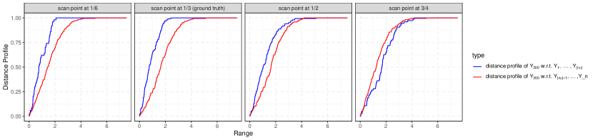
Figure 1: The distance profiles of $Y_{200}$ in the sequence of observations $Y_{i},\ i=1,\dots,300$, where $Y_{i}\sim N(0,1),\ i=1,\dots,100$ and $Y_{i}\sim N(2,1),\ i=101,\dots,300$ with respect to $Y_{1},\dots,Y_{[nu]}$ and $Y_{[nu]+1},\dots,Y_{n}$ at different scan points $u=\frac{1}{6},\frac{1}{3}\text{(the change point)},\frac{1}{2},\frac{3}{4}$.

In order to construct an asymptotic level $\alpha$ test we derive the distribution of the test statistic (2.4) under $H_{0}$ (2.1) in Theorem 1 which needs the following assumptions.

1. Let $F_{\omega}^{(1)}(t)=\mathbb{P}(d(\omega,Y)\leq t)$, where $Y\sim P_{1}$, and $F_{\omega}^{(2)}(t)=\mathbb{P}(d(x,Y^{\prime})\leq t)$, where $Y^{\prime}\sim P_{2}$. Assume that $F_{\omega}^{(1)}(t)$ and $F_{\omega}^{(2)}(t)$ are absolutely continuous for each $\omega\in\Omega$, with densities given by $f_{\omega}^{(1)}(t)$ and $f_{\omega}^{(2)}(t)$ respectively. Assume that there exists $L_{1},L_{2}>0$ such that $\sup_{\omega\in\Omega}\sup_{t\in\mathbb{R}}|f_{\omega}^{(1)}(t)|\leq L_{1}$ and $\sup_{\omega\in\Omega}\sup_{t\in\mathbb{R}}|f_{\omega}^{(2)}(t)|\leq L_{2}$. Moreover assume that $\inf_{t\in\mathrm{supp}(f^{(1)}_{\omega})}f^{(1)}_{\omega}(t)>0$ and $\inf_{t\in\mathrm{supp}(f^{(2)}_{\omega})}f^{(2)}_{\omega}(t)>0$ for each $\omega\in\Omega$.

2. Let $N(\epsilon,\Omega,d)$ be the covering number of the space $\Omega$ with balls of radius $\epsilon$ and $\log N(\epsilon,\Omega,d)$ the corresponding metric entropy, which satisfies

   $$\epsilon\log N(\epsilon,\Omega,d)\rightarrow 0\quad\text{as}\quad\epsilon\rightarrow 0.$$ (2.5)

Assumption (A1) imposes regularity conditions on the distance profiles under the distributions $P_{1}$ and $P_{2}$. Assumption (A2) constrains the complexity of the metric space $(\Omega,d)$ and is applicable to a wide range of spaces including any space $\Omega$ which can be represented as a subset of elements in a finite dimensional Euclidean space, for example networks (Kolaczyk et al., 2020; Ginestet et al., 2017), simplex valued objects in a fixed dimension (Jeon and Park, 2020; Chen et al., 2012) and the space of phylogenetic trees with the same number of tips (Kim et al., 2020; Billera et al., 2001). Assumption (A2) holds for any $\Omega$ which is a VC-class of sets or a VC-class of functions (Theorems 2.6.4 and 2.6.7, Van Der Vaart et al., 1996), for $p$-dimensional smooth function classes $C_{1}^{\alpha}(\mathcal{X})$ (page 155, Van Der Vaart et al., 1996) on bounded convex sets $\mathcal{X}$ in $\mathbb{R}^{p}$ equipped with the $\|\cdot\|_{\infty}$-norm (Theorem 2.7.1, Van Der Vaart et al., 1996) and $\|\cdot\|_{r,Q}$-norm for any probability measure $Q$ on $\mathbb{R}^{p}$ (Corollary 2.7.2, Van Der Vaart et al., 1996) if $\alpha\geq p+1$ and for the case when $\Omega$ is the space of one-dimensional distributions on some compact interval $I\subset\mathbb{R}$ that are absolutely continuous with respect to the Lebesgue measure on $I$ with smooth uniformly bounded densities and $d=d_{W}$ with $d_{W}$ being the 2-Wasserstein metric (Dubey et al., 2022). In fact Assumption (A2) is satisfied when $\Omega$ is the space of $p$-dimensional distributions on a compact convex set $I\subset\mathbb{R}^{p}$, represented using their distribution functions endowed with the $L_{r}$ metric with respect to the Lebesgue measure on $I$ if $\Omega\subset C_{1}^{\alpha}(I)$ for $\alpha\geq p+1$. Next we present Theorem (1) which establishes the null distribution of the test statistic (2.4) as $n\rightarrow\infty$ as the law of the random variable $\mathcal{T}$ as introduced in the same theorem.

Theorem 1.

Under $H_{0}$ and assumptions (A1) and (A2), as $n\rightarrow\infty$, $\hat{T}_{n}$ converges in distribution to the law of a random variable $\mathcal{T}=\sup_{u\in\mathcal{I}_{c}}\sum_{j=1}^{\infty}\mathbb{E}_{Y}\{\lambda_{j}^{Y}\}\mathcal{G}_{j}^{2}(u)$, where $Y\sim P_{1}$, $\lambda^{x}_{1}\geq\lambda^{x}_{1}\geq\dots$ correspond to the eigenvalues of the covariance function given by $C_{x}(t_{1},t_{2})=\mathrm{Cov}\left(\mathbb{I}\left\{d(x,Y)\leq t_{1}\right\},\mathbb{I}\left\{d(x,Y)\leq t_{2}\right\}\right)$ and $\mathcal{G}_{1},\mathcal{G}_{2},\dots$ are independent zero mean Gaussian processes with covariance given by $c(u_{1},u_{2})=\sqrt{\frac{(1-u_{1})(1-u_{2})}{u_{1}u_{2}}}\min(u_{1},u_{2})+\sqrt{\frac{u_{1}u_{2}}{(1-u_{1})(1-u_{2})}}\min(1-u_{1},1-u_{2})$.

Here we discuss the major bottleneck that we needed to overcome in proving Theorem 1 and relegate the technical details to the Supplement. Since the goal is to have a sample-splitting free test, we use the same observations $Y_{1},\dots,Y_{n}$ to estimate the distance profiles and thereafter to estimate the scan statistic that makes each summand in (2.3) significantly dependent on each other. To obtain the null distribution in Theorem 1 we decompose the test statistic (2.4) into several parts, some of which contribute to the asymptotic null distribution while we that the others are asymptotically negligible using maximal inequalities from U-process theory.

For a level $\alpha$ test, we propose to reject $H_{0}$ (2.1) if $\hat{T}_{n}>q_{\alpha}$ where $q_{\alpha}$ is the $(1-\alpha)$-quantile of $\mathcal{T}$. Equivalently one rejects $H_{0}$ when ${p}\leq\alpha$ where ${p}=\mathbb{P}_{H_{0}}(\mathcal{T}\geq\hat{T}_{n})$ is the asymptotic p value of the test. Unfortunately, the law of $\mathcal{T}$ depends on the underlying data distribution and the rejection region, either using the critical value $q_{\alpha}$ or the p value ${p}$ must be approximated in practice. Staying in line with adopted conventions we adopt a random permutation scheme to obtain this approximation that is described next and later design a framework in Section 2.4 to study the power of the test using this approximation scheme in large samples.

Let $\Pi$ denote the collection of $n!$ permutations of $\{1,2,\dots,n\}$. Let $\pi_{0}=(\pi_{0}(1),\dots,\pi_{0}(n))$ be the identity permutation such that $\pi_{0}(j)=j$ for $j=1,\dots,n$ and $\pi_{1},\pi_{2},\dots,\pi_{K}$ be $K$ i.i.d samples from the uniform distribution over $\Pi$ where each $\pi_{k}=(\pi_{k}(1),\dots,\pi_{k}(n))$ is a permutation of $\{1,\dots,n\}$. For each $k=0,1,2,\dots$, let $\hat{T}^{\pi_{k}}_{n}$ be the test statistic evaluated on a reordering of the data given by $Y_{\pi_{k}(1)},\dots,Y_{\pi_{k}(n)}$. Then the permutation p value is given by $\hat{p}_{K}=\frac{1}{K+1}\sum_{k=0}^{K}\mathbb{I}\left\{\hat{T}^{\pi_{k}}_{n}\geq\hat{T}_{n}\right\}$ and the test is rejected at level $\alpha$ when $\hat{p}_{K}\leq\alpha$. It is easy to see that under $H_{0}$ (2.1), $\hat{p}_{K}$ as an approximation of $p$ controls the type I error of the test at level $\alpha$ with high probability for sufficiently large $K$ (see Chung and Romano, (2016)).

2.4 Power analysis under contiguous alternatives

We will study the large sample power of the test, first assuming that the asymptotic critical value $q_{\alpha}$ is available, and thereafter using the practicable permutation scheme for the test. A few definitions are in order before we can state our results. For $t\in\mathbb{R}$ and a random object $Y$, where it is possible that either $Y\sim P_{1}$ or $Y\sim P_{2}$, let ${F}^{(1)}_{{Y}}(t)=\mathbb{P}_{Y^{\prime}}\left(d(Y,Y^{\prime})\leq t\right)$ with $Y^{\prime}\sim P_{1}$ and ${F}^{(2)}_{{Y}}(t)=\mathbb{P}_{Y^{\prime\prime}}\left(d(Y,Y^{\prime\prime})\leq t\right)$ with $Y^{\prime\prime}\sim P_{2}$ and both $Y^{\prime}$ and $Y^{\prime\prime}$ are independent of $Y$. Define the quantity $\Delta=\Delta(P_{1},P_{2})$ as

$$\Delta=\mathbb{E}_{Y\sim P_{1}}\left(\int_{0}^{\mathcal{M}}\left\{{F}^{(1)}_{{Y}}(t)-{F}^{(2)}_{{Y}}(t)\right\}^{2}dt\right)+\mathbb{E}_{Y\sim P_{2}}\left(\int_{0}^{\mathcal{M}}\left\{{F}^{(1)}_{{Y}}(t)-{F}^{(2)}_{{Y}}(t)\right\}^{2}dt\right)$$ (2.6)

where $\mathcal{M}=\mathrm{diam}(\Omega)$ is the diameter of $\Omega$. Immediately one sees that under $H_{0}$ (2.1), $\Delta=0$. In fact $\Delta$ corresponds to the quantity $D^{w}_{XY}$ introduced in Dubey et al., (2022) and under mild conditions $(\Omega,d)$, $P_{1}$ and $P_{2}$, $\Delta=0$ if and only if $P_{1}=P_{2}$.

Let $\mathcal{P}_{(\Omega,d)}$ denote the class of all Borel probability measures on $(\Omega,d)$ which are uniquely determined by open balls, that is, for $Q_{1},Q_{2}\in\mathcal{P}_{(\Omega,d)}$, $Q_{1}=Q_{2}$ if and only if $F^{Q_{1}}_{\omega}(t)=F^{Q_{2}}_{\omega}(t)$ for all $\omega\in\Omega$ and $t\in\mathbb{R}$. In fact $\mathcal{P}_{(\Omega,d)}$ contains all Borel probability measures on $(\Omega,d)$ under special conditions on $(\Omega,d)$ such as, for example, when $(\Omega,d^{k})$ is of strong negative type (Lyons, 2013) for some $k>0$ (see Proposition 1 in Dubey et al., (2022)). Then $\Delta=0$ implies that $F_{\omega}^{P_{1}}(u)=F_{\omega}^{P_{2}}(u)$ for almost any $t\in\mathbb{R}$ and for any $\omega$ in the union of the supports of $P_{1}$ and $P_{2}$. Hence if $\Omega$ is contained in the union of the supports of $P_{1}$ and $P_{2}$, then $\Delta=0$ implies that $P_{1}=P_{2}$ whenever $P_{1},P_{2}\in\mathcal{P}_{(\Omega,d)}$ in which case $\Delta$ serves as a divergence measure between $P_{1}$ and $P_{2}$ and can be used to measure the discrepancy between $H_{1}$ (2.2) and $H_{0}$ (2.1).

To investigate the power of the test we consider the challenging case, a sequence of alternatives $H_{1,n}$ that shrinks to $H_{0}$ where

$$H_{1,n}=\left\{(P_{1},P_{2}):\Delta=a_{n}\right\}$$ (2.7)

with $a_{n}\rightarrow 0$ as $n\rightarrow\infty$. In this framework the asymptotic power of a level $\alpha$ test is quantified using

$$\beta^{\alpha}_{n}=\mathbb{P}_{H_{1,n}}\left({p}\leq\alpha\right)$$

where $p$ is the asymptotic p-value and depends on the null distribution of the test described by the law of $\mathcal{T}$ in Theorem 1. Since the law of $\mathcal{T}$ is unknown, we obtain a tractable estimator of $p$ given by $\hat{p}_{K}$ using the permutation scheme, and the practicable power is quantified as

$$\tilde{\beta}^{\alpha}_{n}=\mathbb{P}_{H_{1,n}}\left(\hat{p}_{K}\leq\alpha\right).$$ (2.8)

Theorem 2 gives the asymptotic consistency for any level $\alpha$ test, by showing that the power of the test in both asymptotic and practicable regimes converge to one as $n\rightarrow\infty$ in the hard to detect scenario of contiguous alternatives provided that $na_{n}\rightarrow\infty$, i.e., $a_{n}$ does not decay too fast as $n\rightarrow\infty$.

Theorem 2.

Under assumptions (A1) and (A2), for any $\alpha\in(0,1)$ and as $n\rightarrow\infty$, $\beta^{\alpha}_{n}\rightarrow 1$ as $n\rightarrow\infty$. Moreover if $na_{n}\rightarrow\infty$ and $K\geq\frac{1}{\alpha}$, where $K$ is the total number of permutations used to estimate $\hat{p}_{K}$ in (2.8) then $\tilde{\beta}^{\alpha}_{n}\rightarrow 1$ as $n\rightarrow\infty$.

2.5 Change point estimation

In this section we describe the estimation of $\tau$ when it exists. As a straightforward consequence of our test statistic (2.4) we estimate $\tau$ as

$$\hat{\tau}=\operatorname*{arg\,max}_{u\in\mathcal{I}_{c}}\hat{T}_{n}(u).$$ (2.9)

Next we discuss the asymptotic behavior of $\hat{\tau}$ around $\tau$. For this we consider two scenarios, first, where the alternative is fixed which is the case that is studied typically in nonparametric change point analysis, and then the case where the alternative is such that $(P_{1},P_{2})\in H_{1,n}$ with $H_{1,n}$ as defined in (2.7) such that $\Delta(P_{1},P_{2})=a_{n}$ with $a_{n}\rightarrow 0$ as $n\rightarrow\infty$. The second scenario offers a difficult setup for detecting $\tau$ accurately. In Theorem 3 we show the asymptotic near-optimal rate of convergence for the change point in the first scenario of fixed alternatives when $P_{1}\neq P_{2}$ (Madrid Padilla et al., 2021). In the second situation, the change point estimator $\hat{\tau}$ is a consistent estimator of $\tau$ only if $na_{n}\rightarrow\infty$ as $n\rightarrow\infty$, which is also the requirement for the consistency of the test as per Theorem 2.

Theorem 3.

For any fixed alternative when $P_{1}\neq P_{2}$, under assumptions (A1) and (A2), as $n\rightarrow\infty$,

$$\lvert\hat{\tau}-\tau\rvert=O_{P}\left(\frac{\log(n)}{n}\right).$$

For the contiguous alternatives $H_{1,n}$, there exists $L>0$ such that $\mathbb{P}_{H_{1,n}}\left({na_{n}}\lvert\hat{\tau}-\tau\rvert\geq L\right)\rightarrow 0$ as $n\rightarrow\infty$.

3 Simulations

We assess the finite sample performance of the our approach across various frameworks involving three different random object spaces. First we carry out extensive simulations capturing diverse change point scenarios in sequences of Euclidean random vectors, then we study change points in bivariate distributional data sequences where the bivariate distributions are equipped with the $L^{2}$ metric between corresponding the cdfs, and finally move on to change points in random network sequences where the networks are represented as graph Laplacians with the Frobenius metric between them and are generated from a preferential attachment model (Barabási and Albert, 1999). For each random object we explore a range of alternatives beyond location shifts and scale shifts, such as, sudden changes in the tails of the population distribution, the population distribution abruptly switching to a mixture distribution with two components and abrupt changes in network node attachment mechanisms.

We generate random object sequences of length $n=300$ and set the level $\alpha$ of the test to be $\alpha=0.05$. In each scenario, we first calibrate the type I error of the new test under $H_{0}$ and then evaluate the empirical power of the test for a succession of alternatives that capture increasing discrepancies between the distributions of the two data segments before and after the change point with $\tau=1/3$. We employ our scan statistic on the interval $\mathcal{I}_{c}=[0.1,0.9]$. We conduct 500 Monte Carlo runs and set the empirical power to be the proportion of the rejections at $\alpha=0.05$ out of the $500$ Monte Carlo runs. The critical value of is approximated using the permutation scheme described in Section 2.3 with $1000$ permutations within each Monte Carlo run. To demonstrate our findings we present empirical power plots where we expect that the empirical power will be maintained at the level $\alpha=0.05$ under $H_{0}$ and will increase with increasing disparities between the the two data segments. Along with the power trends we also investigate the accuracy of the estimated change point locations using their mean absolute deviation (MAE), calculated as

$$\textup{MAE}=\frac{1}{500}\sum_{i=1}^{500}|\hat{\tau}_{i}-\tau|,$$

where $\hat{\tau}_{i}$ is the estimated change point location in the $i$-th Monte Carlo run. We expect that a successful method will have better accuracy in detecting change points, and therefore, have lower MAE with higher distributional differences between the data segments.

We compare the power and the MAE of our test statistic, which we will refer to as “dist-CP” here on, with the energy-based change point detection test (“energy-CP”)(Matteson and James, 2014), graph-based change point detection test (“graph-CP”)(Chen and Zhang, 2015; Chu and Chen, 2019), and kernel-based change point detection test (“kernel-CP”) (Harchaoui et al., 2008; Jones and Harchaoui, 2020). We adopt the same configuration whenever needed for each of these tests, for example, we set the number of permutations to be 1000 to obtain the p-value approximations. For the graph-based test, we apply the generalized edge-count scan statistic (Chu and Chen, 2019) and choose 5-MST (minimum spanning tree) to construct the initial similarity graph as suggested by Chen and Zhang, (2015). For the kernel-CP, we use the Gaussian kernel and select the bandwidth to be the median of the input pairwise distances. In terms of the implementation, we use the R packages “gSeg”(chen:2020) and “ecp”(Jame:2015) for graph-CP and energy-CP separately, and Python package “Chapydette”(Jones and Harchaoui, 2020) for kernel-CP.

3.1 Multivariate data

In this setting the data elements are random vectors endowed with $l^{2}$ metric and are generated from the $p$-dimensional Gaussian distribution $N(\mu,\Sigma)$ with mean $\mu$ and covariance matrix given by $\Sigma$. We explore four different types of changes to the population distributions, which we summarize in Table 1. First we consider location and scale changes , in dimensions $p=30,90$ and $180$ where to study location change, we set $\mu=\mathbf{0}_{p}=(0,0,\dots,0)^{T}$ for $Y_{i},\ i=1,\dots,100$ and $\mu=\Delta_{1}\mathbf{1}_{p}=\Delta_{1}(1,1,\dots,1)^{T}$ for $Y_{i},\ i=101,\dots,300$, where we let $\Delta_{1}$ range from 0 to 1. The covariance matrix is fixed and constructed as $\Sigma=U\Lambda U^{T}$, where $\Lambda$ is a diagonal matrix with $k$-th diagonal entry being $\textup{cos}(k\pi/p)+1.5$ for $k=1,\dots,p$, and $U$ is an orthogonal matrix with the first columns being $p^{-1/2}(1,1,\dots,1)^{T}$, such that the mean change loads along the first eigenvector of the data. To investigate scale change, we fix the $\mu=\mathbf{0}_{p}$ and set $\Sigma=0.8\mathbf{I}_{p}$ for $Y_{i},\ i=1,\dots,100$ and $\Sigma=(0.8-\Delta_{2})\mathbf{I}_{p}$ for $Y_{i},\ i=101,\dots,300$, where we let $\Delta_{2}$ range from 0 to 0.4. We present the results of location and scale shifts in Figure 2, where Figure 2(a) illustrates the empirical power performances of the tests and Figure 2(b) shows the MAE of estimated change points. In Figure 3, we present the corresponding results for scale change. In Figure 2(a), we see that all the methods maintain type I error control. Energy-CP outperforms the other methods in terms of power and MAE but dist-CP has competitive power performance across all different settings in the mean change scenario. For scale changes, dist-CP has the best performance in terms of both empirical power and MAE across all settings as illustrated in Figure 3.

$P_{1}$ $(Y_{1},\dots,Y_{100}\sim P_{1})$	$P_{2}$ $(Y_{101},\dots,Y_{300}\sim P_{2})$
$N(\mathbf{0}_{p},\Sigma)$ with $\Sigma=Q\Lambda Q^{T}$, where $\Lambda$ is a diagonal matrix with $i$th entry $\cos(i\pi/p)+1.5$ for $i=1,\dots,p$ and $Q$ is an orthogonal matrix whose first column is $p^{-1/2}(1,1,\dots,1)^{T}$	$N(\Delta_{1}\mathbf{1}_{p},\Sigma)$, where $\Delta_{1}\in[0,1]$
$N(\mathbf{0}_{p},\Sigma)$, $\Sigma=0.8\mathbf{I}_{p}$	$N(\mathbf{0}_{p},\Sigma)$, where $\Sigma=(0.8-\Delta_{2})\mathbf{I}_{p}$ and $\Delta_{2}\in[0,0.4]$
$N(\mathbf{0}_{p},\mathbf{I}_{p})$	$AZ_{1}+(1-A)Z_{2}$, where $A\sim\textup{Bernoulli(0.5)}$, $Z_{1}\sim N(-\mu,\mathbf{I}_{p})$, $Z_{2}\sim N(\mu,\mathbf{I}_{p})$, where $\mu=(\Delta_{3}\mathbf{1}_{0.1p},\mathbf{0}_{0.9p})^{T}$, where $\Delta_{3}\in[0,1]$ and $A$, $Z_{1}$, and $Z_{2}$ are independent.
$N(\mathbf{0}_{p},\mathbf{I}_{p})$	$p$-dimensional random vectors whose components are independent and identically distributed as the t-distribution bluewith $v$ degrees of freedom, where $v\in\{2,\dots,22\}$

Table 1: Different change point scenarios when $\Omega=\mathbb{R}^{p}$ equipped with metric $d=||x-y||_{2}$ for $x,y\in\Omega$. Going from top to bottom, the successive rows encode population mean change, population scale change, the population distribution separating into distinct mixture components and the population distribution changing to being heavy-tailed.

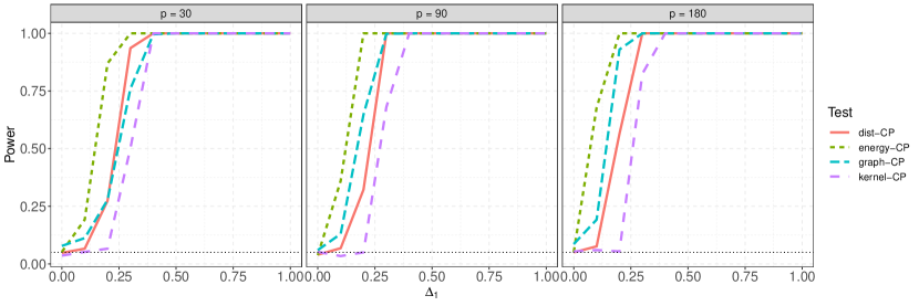
(a)

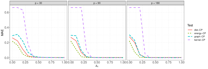
(b)

Figure 2: In Figure 2(a), we present the power comparisons with respect to $\Delta_{1}$ (see Table 1) for a sequence of $p$- dimensional random vectors sampled from $N(\mu,\Sigma)$, where $\mu=\mathbf{0}_{p}=(0,0,\dots,0)^{T}$ for $Y_{i},\ i=1,\dots,100$ and $\mu=\Delta_{1}\mathbf{1}_{p}=\Delta_{1}(1,1,\dots,1)^{T}$ for $Y_{i},\ i=101,\dots,300$. $\Sigma$ is held fixed for the whole sequence as $\Sigma=U\Lambda U^{T}$, where $\Lambda$ is a diagonal matrix with $k$th diagonal entry being $\textup{cos}(k\pi/p)+1.5$ for $k=1,\dots,p$, and $U$ is an orthogonal matrix with the first columns being $p^{-1/2}(1,1,\dots,1)^{T}$. The dotted black line indicates the significance level of 0.05. Figure 2(b) presents the MAE of the estimated change points with respect to $\Delta_{1}$.

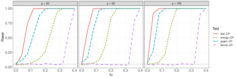
(a)

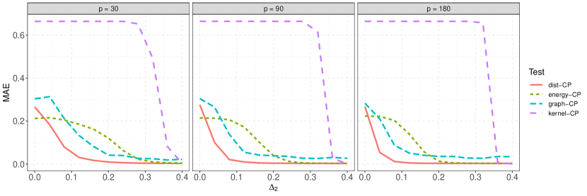
(b)

Figure 3: In Figure 3(a), we present the power comparisons with respect to $\Delta_{2}$ (see Table 1) for a sequence of $p$- dimensional random vectors sampled from $N(\mu,\Sigma)$, where $\mu=\mathbf{0}_{p}$ for the whole sequence. $\Sigma=0.8\mathbf{I}_{p}$ for $Y_{i},\ i=1,\dots,100$ and $\Sigma=(0.8-\Delta_{2})\mathbf{I}_{p}$ for $Y_{i},\ i=101,\dots,300$. The dotted black line indicates the significance level of 0.05. Figure 3(b) presents the MAE of the estimated change points with respect to $\Delta_{2}$.

Next we study sudden splitting of a homogeneous population into a mixture of two components with different means. To study this we take $Y_{1},\dots,Y_{100}$ to be generated from the standard $p$-dimensional Gaussian distribution $N(\mathbf{0}_{p},\mathbf{I}_{p})$ and let $Y_{101},\dots,Y_{300}$ be generated from a mixture of two Gaussian distributions with the overall population mean same as $Y_{1},\dots,Y_{100}$. To be more specific, $Y_{101},\dots,Y_{300}$ are constructed with independent samples of $AZ_{1}+(1-A)Z_{2}$, where $A\sim\textup{Bernoulli(0.5)}$, $Z_{1}\sim N(-\mu,\mathbf{I}_{p})$, $Z_{2}\sim N(\mu,\mathbf{I}_{p})$, where $\mu=(\Delta_{3}\mathbf{1}_{0.1p},\mathbf{0}_{0.9p})^{T}$, and $A$, $Z_{1}$, and $Z_{2}$ are independent. Here, $\Delta_{3}\in[0,1]$. In Figure 4 we illustrate that dist-CP outperforms all other approaches both in terms of empirical power and MAE in this complex change point scenario.

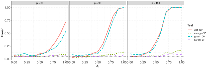
(a)

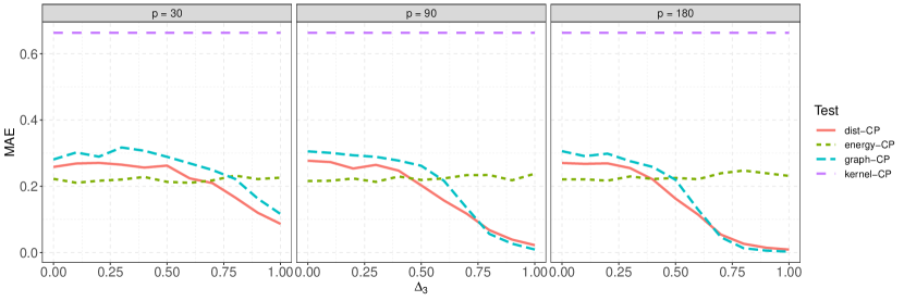
(b)

Figure 4: In Figure 4(a), we present the power comparisons with respect to $\Delta_{3}$(see Table 1) for a sequence of $p$ dimensional random vectors. Here, $Y_{1},\dots,Y_{100}$ are generated from the standard $p$ dimensional Gaussian distribution $N(\mathbf{0}_{p},\mathbf{I}_{p})$. $Y_{101},\dots,Y_{300}$ are constructed with independent samples of $AZ_{1}+(1-A)Z_{2}$, where $A\sim\textup{Bernoulli(0.5)}$, $Z_{1}\sim N(-\mu,\mathbf{I}_{p})$, $Z_{2}\sim N(\mu,\mathbf{I}_{p})$, where $\mu=(\Delta_{3}\mathbf{1}_{0.1p},\mathbf{0}_{0.9p})^{T}$, and $A$, $Z_{1}$, and $Z_{2}$ are independent. The dotted black line indicates the significance level of 0.05. Figure 4(b) presents the MAE of the estimated change points with respect to $\Delta_{3}$

Finally we experiment with changes to the tail of the population distribution. We generate $Y_{i}\sim N(\mathbf{0}_{p},\mathbf{I}_{p})$ with $p\in\{5,15,60\}$ for $i=1,\dots,100$ and $Y_{i}$ as a $p$-dimensional random vector whose components are independent and identically distributed as the t-distribution with $v$ degrees of freedom for $i=101,\dots,300$ We let $v$ range in $\{2,\dots,22\}$ to reflect the change from Gaussian tails to successively heavier tails. The results as shown in Figure 5 demonstrate that dist-CP has the best power and MAE performance across all settings.

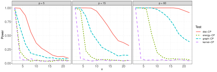
(a)

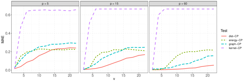
(b)

Figure 5: In Figure 5(a), we present the power comparison for increasing values of $v$ (see Table 1) for a sequence of $p$ dimensional random vectors. Here, $Y_{i}\sim N(\mathbf{0}_{p},\mathbf{I}_{p})$ with $p\in\{5,15,60\}$ for $i=1,\dots,100$ and $Y_{i}\sim t_{v}$ for $i=101,\dots,300$, where $t_{v}$ stands for $t$ distribution with $v$ degrees of freedom. The dotted black line indicates the significance level of 0.05. Figure 5(b) presents the MAE of the estimated change points with respect to $v$.

3.2 Bivariate distributional data

Here the random objects are random bivariate probability distributions equipped with the metric between corresponding cumulative distribution function representations defined as $d(x,y)=\int_{\mathbb{R}}\int_{\mathbb{R}}|F_{x}(u,v)-F_{y}(u,v)|\ dudv$, where $F_{x}(u,v)$ is the bivariate cdf of $x$. Each observation $Y_{i}$ for $i=1,\dots,300$ is itself a bivariate distribution with a cdf representation where we explore two types of changes: changes in the process generating the means of $Y_{i}$ and changes in the process generating the variances in the covariance structure of $Y_{i}$. We provide a summary of the changes in Table 2. Specifically, for the first scenario, $Y_{i}=N(Z_{i},0.25\mathbf{I}_{2})$, where $Z_{i}\sim N(\mathbf{0}_{2},0.25\mathbf{I}_{2})$ for $i=1,\dots,100$, and $Z_{i}\sim N((\delta_{1},0)^{T},0.25\mathbf{I}_{2})$ for $i=101,\dots,300$ where $\delta_{1}\in[0,1]$. For changes in the scales of the random distributions we generate $Y_{i}=N(Z_{i},0.25\mathbf{I}_{2})$, where $Z_{i}\sim N(\mathbf{0}_{2},0.4^{2}\mathbf{I}_{2})$ for $i=1,\dots,100$, and $Z_{i}\sim N(\mathbf{0}_{2},\textup{diag}((0.4+\delta_{2})^{2},0.4^{2}))$ for $i=101,\dots,300$ and let $\delta_{2}\in[0,4]$. We illustrate our findings in 6 and 7. In Figure 6, dist-CP, energy-CP, and kernel-CP have similar performance and are better than graph-CP in terms of both power and MAE. In the second case, dist-CP dominates the performance across all settings.

$P_{1}$ $(Y_{1},\dots,Y_{100}\sim P_{1})$	$P_{2}$ $(Y_{101},\dots,Y_{300}\sim P_{2})$
$Y_{i}=N(Z_{i},0.25\mathbf{I}_{2})$ with $Z_{i}\sim N(\mathbf{0}_{2},0.25\mathbf{I}_{2})$	$Y_{i}=N(Z_{i},0.25\mathbf{I}_{2})$ with $Z_{i}\sim N((\delta_{1},0)^{T},0.25\mathbf{I}_{2})$, and $\delta_{1}\in[0,1]$
$Y_{i}=N(Z_{i},0.25\mathbf{I}_{2})$ with $Z_{i}\sim N(\mathbf{0}_{2},0.4^{2}\mathbf{I}_{2})$	$Y_{i}=N(Z_{i},0.25\mathbf{I}_{2})$ with $Z_{i}\sim N(\mathbf{0}_{2},\textup{diag}((0.4+\delta_{2})^{2},0.4^{2}))$, and $\delta_{2}\in[0,0.4]$

Table 2: Different change point scenarios for $\Omega=\{(u,v)\mapsto F(u,v):F(\cdot,\cdot)\ \text{is a bivariate cdf}\}$ equipped with the metric $d=\int_{\mathbb{R}}\int_{\mathbb{R}}|F_{x}(u,v)-F_{y}(u,v)|\ dudv$ for $F_{x},F_{y}\in\Omega$. The first row describes a change in the distribution of the mean of each $Y_{i}$ and the second row describes a change in the distribution of scale aspects of each $Y_{i}$.

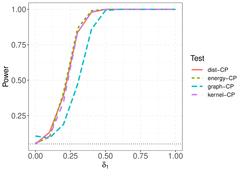
(a)

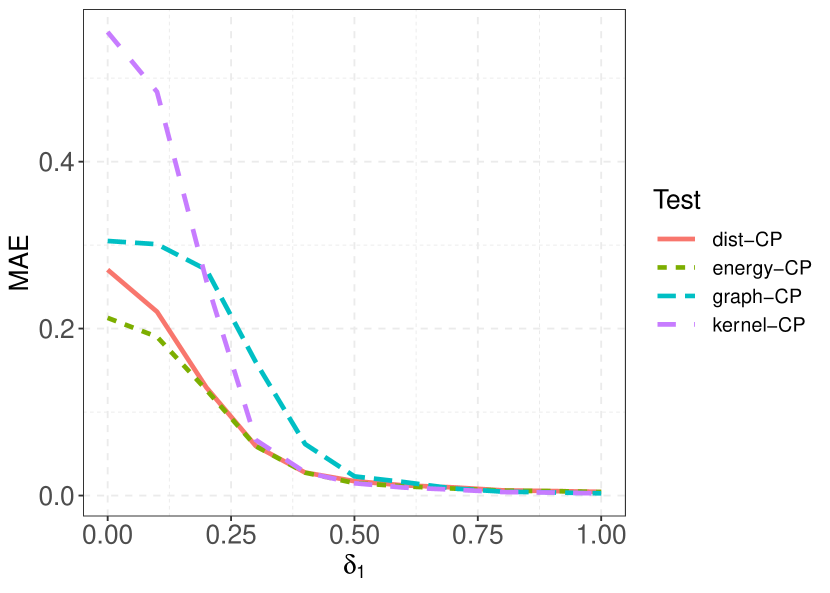
(b)

Figure 6: In Figure 6(a), we present the power comparisons with respect to $\delta_{1}$ (see Table 2) for a sequence of bivariate Gaussian distributional data. Here, $Y_{i}=N(Z_{i},0.25\mathbf{I}_{2})$, where $Z_{i}\sim N(\mathbf{0}_{2},0.25\mathbf{I}_{2})$ for $i=1,\dots,100$, and $Z_{i}\sim N((\delta_{1},0)^{T},0.25\mathbf{I}_{2})$ for $i=101,\dots,300$. The dotted black line indicates the significance level of 0.05. Figure 6(b) presents the MAE of the estimated change points with respect to $\delta_{1}$.

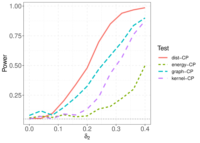
(a)

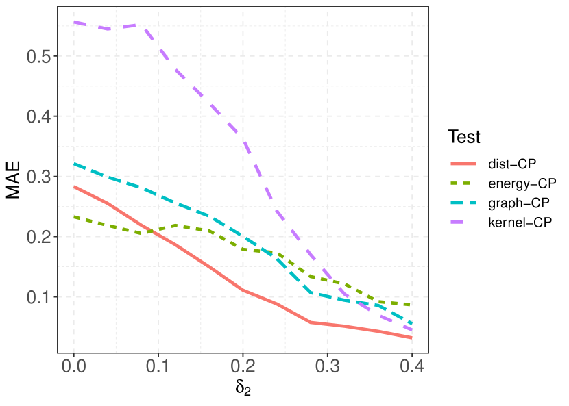
(b)

Figure 7: In Figure 7(a), we present the power comparison for increasing values of $\delta_{2}$ (see Table 2) for a sequence of bivariate Gaussian distributional data. Here, $Y_{i}=N(Z_{i},0.25\mathbf{I}_{2})$, where $Z_{i}\sim N(\mathbf{0}_{2},0.4^{2}\mathbf{I}_{2})$ for $i=1,\dots,100$, and $Z_{i}\sim N(\mathbf{0}_{2},\textup{diag}((0.4+\delta_{2})^{2},0.4^{2}))$ for $i=101,\dots,300$. The dotted black line indicates the significance level of 0.05. Figure 7(b) presents the MAE of the estimated change points with respect to $\delta_{2}$.

3.3 Network data

Lastly, we consider random object sequences where the data elements are random networks endowed with the Frobenius metric between the corresponding Laplacian matrix. Each $Y_{i}$ is a network with $200$ nodes generated from the preferential attachment model (Barabási and Albert, 1999) where for a node with degree $k$, its attachment function is proportional to $k^{\gamma}$. $Y_{i}$ is generated with $\gamma=0$ for $i=1,\dots,100$, and $Y_{i}$ is generated with $\gamma$ from 0 to 0.5 for $i=101,\dots,300$. We summarize the settings in Table 3, and present the simulation results in Figure 8. dist-CP outperforms the other methods in both power and change point location estimation MAE.

$P_{1}$ $(Y_{1},\dots,Y_{100}\sim P_{1})$	$P_{2}$ $(Y_{101},\dots,Y_{100}\sim P_{2})$
networks generated from preferential attachment model with $\gamma=0$	networks generated from preferential attachment model with $\gamma\in[0,0.5]$

Table 3: Change point scenario where $\Omega=\{\textup{graph laplacians of networks with 200 nodes}\}$ equipped with metric $d(L_{1},L_{2})=\sqrt{\textup{trace}((L_{1}-L_{2})^{T}(L_{1}-L_{2}))}$ for $L_{1},L_{2}\in\Omega$.

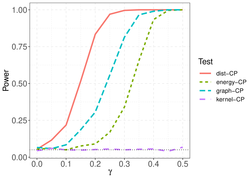
(a)

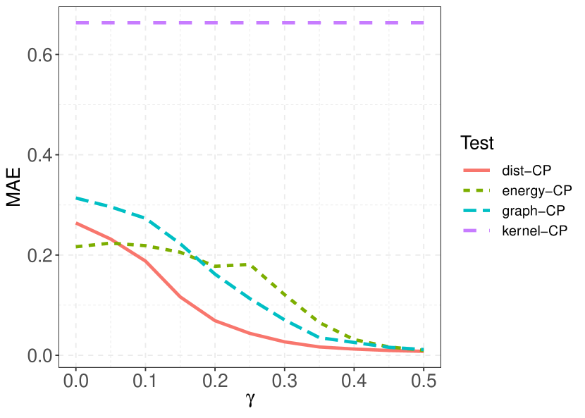
(b)

Figure 8: In Figure 8(a), we present the power comparisons with respect to increasing values $\gamma$ (see Table 3) for a sequence of random networks with 200 nodes generated by the preferential attachment model. For a node with degree $k$, its attachment function is proportional to $k^{\gamma}$. $Y_{i}$ is generated with $\gamma=0$ for $i=1,\dots,100$, and $Y_{i}$ is generated with $\gamma\in[0,0.5]$ for $i=101,\dots,300$. The dotted black line indicates the significance level of 0.05. Figure 8(b) presents the MAE of the estimated change points with respect to $\gamma$.

4 Data applications

4.1 U.S. electricity generation dataset

We analyze the monthly U.S. electricity generation compositions obtained from https://www.eia.gov/electricity/data/browser/. We preprocess the data elements into a compositional form so that each entry of the compositional vector represents the percentage of net generation contribution from a specific source. During the preprocessing, we merge some similar categories of resources together and end up with 7 categories: Coal; Petroleum (petroleum liquids and petroleum coke); Gas (natural and other gases); Nuclear; Conventional hydroelectric; Renewables (wind, geothermal, biomass (total) and other); Solar (small-scale solar photovoltaic and all utility-scale solar). We obtain a sample of $n=264$ observations starting from Jan 2001 to Dec 2022. Each $Y_{i}$ takes values in a 6-simplex $\Delta^{6}=\{\bm{x}\in\mathbb{R}^{7}:\bm{x}^{T}\mathbf{1}_{7}=1\}$, where $\mathbf{1}_{7}=(1,1,\dots,1)^{T}$. The metric we apply between each object is

$$d(\bm{x},\bm{y})=\textup{arccos}(\sqrt{\bm{x}}^{T}\sqrt{\bm{y}}),\quad\bm{x},\bm{y}\in\mathbb{R}^{7},$$

where $\sqrt{\bm{x}}$ is the component-wise square root, i.e., $\sqrt{\bm{x}}=(\sqrt{x_{1}},\sqrt{x_{2}},\dots,\sqrt{x_{7}})$.

We apply dist-CP to the preprocessed data and present the plot of the scan statistic in Figure 9. The scan statistic peaks in month of February 2015. In Figure 10, we present the statistically significant estimated change point location with a vertical red dash line. At the change point, we can observe that the percentage of contributions from solar and renewable sources is increasing more rapidly while petroleum contributions drop rapidly. U.S. reached new milestones in renewables electricity generation in the year 2015 (see https://obamawhitehouse.archives.gov/blog/2016/01/13/renewable-electricity-progress-accelerated-2015)which explains the detected change point.

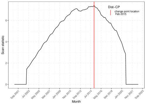
Figure 9: The scan statistic for the monthly U.S. electricity compositions data. The vertical red line indicates the location of the estimated change point in the month of February 2015.

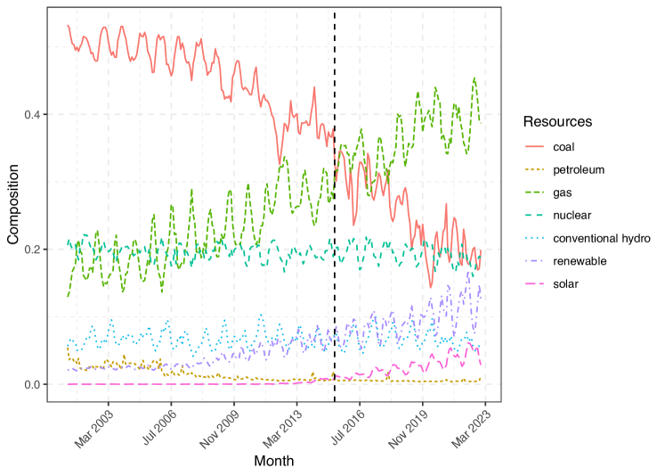
Figure 10: The timeline of U.S. electricity compositions evolution and the change point February 2015 indicated by the vertical dashed black line.

4.2 MIT reality mining dataset

The MIT Media Laboratory conducted the reality mining experiment from 2004 to 2005 on students and faculty at MIT (Eagle and Pentland, 2006) in order to explore human interactions based on Bluetooth and other phone applications’ activities. We study the participants’ Bluetooth proximity networks, where nodes represent participants and the edges represent whether the relevant participants had at least one physical interaction within the time interval.

We use the reality mining 1392 built-in dataset in the R package “GreedySBTM” (Rast:2019) (see https://github.com/cran/GreedySBTM/blob/master/data/reality_mining_1392.RData). The time frames corresponding to intervals of 4 hours, starting from September 14 2004 to May 5 2005. At each time point the network has $=96$ nodes. We further compressed the data by merging the time windows with a day to obtain 232 daily networks. We work with the pairwise Frobenius metric between the graph Laplacian representation of the networks. Using dist-CP the estimated change point is 2004-12-15, which is during the finals week and close to the start of the winter break. We present the scan statistics for the whole sequence in Figure 11.

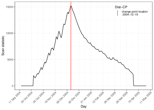
Figure 11: The scan statistic for MIT reality mining dataset. The vertical red line indicates the estimated change point 2004-12-15 which is during the finals week and around the beginning of the winter break.

5 Multiple change points

In this section, we investigate the extension of dist-CP to the task of detecting multiple change points. We combine our test statistic with the recently proposed seeded binary segmentation algorithm (Kovács et al., 2023), an approach that shares similar ideas with the wild binary segmentation (Fryzlewicz, 2014). Seeded binary segmentation controls the computational cost in a near-linear time by creating a collection of seeded intervals $\mathcal{I}_{\gamma}$ which removes unnecessarily long intervals in wild binary segmentation that might contain multiple change points. As introduced in Kovács et al., (2023), for a sequence of length $n$, the collection of intervals $\mathcal{I}_{\gamma}$ is given by

$$\mathcal{I}_{\gamma}=\bigcup_{k=1}^{\lceil\log_{1/\gamma}(n)\rceil}\mathcal{I}_{k}$$ (5.1)

where $\gamma\in[1/2,1)$ is a decay parameter, $\mathcal{I}_{k}=\bigcup_{i=1}^{n_{k}}\{(\lfloor(i-1)s_{k}\rfloor),\lfloor(i-1)s_{k}+l_{k}\rfloor\}$ and $n_{k}=2\lceil(1/\gamma)^{k-1}\rceil-1$. Each $\mathcal{I}_{k}$ is also a collection of intervals of length $l_{k}$ that are evenly shifted by $s_{k}$, where $l_{k}=n\gamma^{k-1}$, $s_{k}=(T-l_{k})/(n_{k}-1)$. In algorithm 1, we describe the detailed implementation of the Mcpd_DP, the multiple change point detection algorithm based on the combination of distance profiles and seeded binary segmentation. Once we obtain $\mathcal{I}_{\gamma}$, we conduct “dist-CP” on each of the inner intervals thus deriving a set of potential change point locations. We compare the test statistic in each inner interval of $\mathcal{I}_{\gamma}$ with a threshold which is set at 90%-quantile of the permutation null distribution of the test statistic derived on the entire sequence in the current implementation. The selection rule is to keep intervals in which the test statistic is greater than the above threshold and remove all the other intervals sequentially until the maximum test statistic in the entire collection of remaining intervals does not exceed the threshold. In the experiments, we set $\gamma={1/2}^{1/2}$ as suggested by Kovács et al., (2023) and set minLen to be 10.

Algorithm 1 Multiple change point detection based on distance profile: Mcpd_DP

Input: $l$ and $u$: lower and upper boundaries of the original sequence, minLen: minimum length of each interval, $\gamma$: decay parameter, intial change point set $\hat{\tau}=\emptyset$
Output: detected change point set $\hat{\tau}$

1:procedure Mcpd_DP($l$,$u$,$\gamma$,$\hat{\tau}$,minLen)

2:     if $u-l<$minLen then STOP.

3:     calculate the seeded interval collection $\mathcal{I}_{\gamma}$ as described in equation 5.1.

4:     for i in 1 to $|\mathcal{I}_{\gamma}|$ do

5:         denote $u_{i}$ and $l_{i}$ the upper and lower boundaries of the $i$th interval in $\mathcal{I}_{\gamma}$.

6:         denote the proposed test statistics on interval $[l_{i},u_{i}]$ as $\hat{T}_{i}$ and record its corresponding estimated change point location as $\hat{t}_{i}$

7:     end for

8:     Let $\Delta$ be the 90% quantile of the approximated permutation distribution based on the entire sample $Y_{1},\dots,Y_{n}$.

9:     if $\max_{i}\hat{T}_{i}>=\Delta$ then

10:         $i^{\prime}\leftarrow\textup{argmax}_{i\in\{1,\dots,|\mathcal{I}_{\gamma}|\}}\hat{T}_{i}$

11:         $\hat{\tau}\leftarrow\hat{\tau}\cup\hat{t}_{i^{\prime}}$

12:         conduct Mcpd_DP($l$,$\hat{t}_{i^{\prime}}$,$\gamma$,$\hat{\tau}$,minLen) and Mcpd_DP($\hat{t}_{i^{\prime}}$,$u$,$\gamma$,$\hat{\tau}$,minLen)

13:     else

14:         break

15:     end if

16:end procedure

5.1 Simulations on network sequences generated using the Stochastic Block Model

To demonstrate the practical efficacy of Mcpd_DP in Algorithm 1, we conduct an experiment on sequences of networks generated according to the stochastic block model (SBM). SBM generates networks with adjacency matrices $A=[A_{ij}]\in\mathbb{R}^{n\times n}$ with $K$ communities, where $A_{ij}\sim\textup{Bernoulli}(P_{ij})$ with $P=[P_{ij}]=\Pi B\Pi^{T}-\text{diag}(\Pi B\Pi^{T})$. Here $\Pi\in\mathbb{R}^{n\times K}$ encodes the community membership of each node, that is, $\Pi_{ik}=1$ if node $i$ belongs to community $k$ and $\Pi_{ik}=0$ otherwise. Here $B\in\mathbb{R}^{K\times K}$ is the connection probability matrix, where $B_{ij}$ indicates the connection probability between $i$-th and $j$-th community. We let $\pi\in\mathbb{R}^{K}$ to be such that $\pi_{i}$ indicates the number of nodes in $i$-th community.

To incorporate different kinds of changes, we focus on the diverse characteristics of the SBM such as changes in the number of nodes in each community and changes in the number of communities. We generate a sequence of networks of length $n=400$ in the SBM framework with change points evenly spaced at $\tau=\{\frac{1}{4},\frac{2}{4},\frac{3}{4}\}$. Specifically $Y_{i}$ are generated with $B=$ $\begin{pmatrix}0.2&0.001&0.001\\ 0.001&0.2&0.001\\ 0.001&0.001&0.2\\ \end{pmatrix}$, and $\pi=(100,100,100)$ for $1\leq i\leq 100$. Then, we change the connecting probability to $B=$ $\begin{pmatrix}0.8&0.001&0.001\\ 0.001&0.2&0.001\\ 0.001&0.001&0.8\\ \end{pmatrix}$, and keep $\pi=(100,100,100)$ the same for $101\leq i\leq 200$. Next, we change $\pi=(200,50,50)$ and keep $B$ the same for $201\leq i\leq 300$. Finally for $301\leq i\leq 400$, we change the number of communities, we set $B=$ $\begin{pmatrix}0.5&0.01\\ 0.01&0.5\\ \end{pmatrix}$ and $\pi=(200,100)$.

We apply Mcpd_DP 1 on the network sequences generated according to the SBM framework described above, and compare the performance with the multiple change points version of energy-CP (Matteson and James, 2014; Jame:2015) and kernel-CP (Arlot et al., 2019). We conduct 500 Monte Carlo runs and evaluate Algorithm 1 on two aspects; first, whether the correct number of change points can be detected and second, conditioning on the correctly estimating the number of change points, on the MAE of the estimated change points. Out of 500 Monte Carlo runs, the proportions of correctly estimating 3 change points are 100%, 95.8% and 100% for the proposed algorithm Mcpd_DP, energy-CP and kernel-CP. All of the three methods achieve zero MAE conditioning on correctly estimating the number of 3 points.

5.2 Multiple change points in real data

Next we illustrate the implementation of Mcpd_DP 1 on the real data examples investigated in Section 4. For the U.S. electricity generation data, Mcpd_DP detects May 2007, February 2015 and February 2019 as the change points as illustrated in Figure 12. In May 2007, while renewable sources pick up suddenly, the petroleum component starts a rapid downward trend alongside abrupt changes in the trends of the coal component. In February 2015 the solar component starts to accelerate along with continuing changes in the renewable component with similar change patterns again in February 2019. For MIT reality mining data, Mcpd_DP 1 detects change points at 2004-10-16 (beginning of sponsor week), 2004-12-16 (around the end of the finals week and beginning of the winter break), 2005-01-01 (starting of the independent activities period) and 2005-03-10 (right after the exam week) according to events labeled in Peel and Clauset, 2015b .

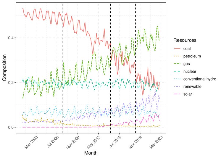
Figure 12: Multiple change points detected for the U.S. electricity generation data. The change points, indicated by the vertical black dashed lines, are at months: May 2007, February 2015 and February 2019.

6 Conclusion

We introduce a nonparametric change point detection method, denoted as dist-CP, designed for random objects taking values in general metric spaces. dist-CP is based solely on pairwise distances and is tuning parameter-free, making it an appealing choice for practitioners working with complex data who seek a straightforward application without the burden of specifying additional parameters except for interval cut-offs where change points are presumed absent. This stands in contrast to other existing approaches for change point detection in metric space data, which typically necessitate parameter choices such as similarity graph selection in graph-CP and kernel and bandwidth selection in kernel-CP. We derive the asymptotic distribution of the test statistic of dist-CP under $H_{0}$ to ensure type I error control and establish the large sample consistency of the test and the estimated change points under contiguous alternatives. We extend all theoretical guarantees to the practicable permutation approximations of the null distribution. Comprehensive simulations across various scenarios, spanning random vectors, distributional data, and networks, showcase the efficacy of dist-CP in many challenging settings, including scale and tail probability changes in Gaussian random vectors and preferential attachment changes in random networks. We study the extension of dist-CP to multiple change point scenarios by combining it with seeded binary segmentation. The data applications lead to insightful findings in the U.S. electricity generation compositions timeline and in the bluetooth proximity networks of the MIT reality mining experiment. With its versatility and minimal parameter requirements dist-CP has the potential for widespread application across various domains as long as distances can be defined between the data elements.

References

- Aminikhanghahi and Cook, (2017) Aminikhanghahi, S. and Cook, D. J. (2017). A survey of methods for time series change point detection. Knowledge and information systems, 51(2):339–367.
- Arlot et al., (2019) Arlot, S., Celisse, A., and Harchaoui, Z. (2019). A kernel multiple change-point algorithm via model selection. Journal of Machine Learning Research, 20(162):1–56.
- Barabási and Albert, (1999) Barabási, A.-L. and Albert, R. (1999). Emergence of scaling in random networks. science, 286(5439):509–512.
- Barassi et al., (2020) Barassi, M., Horvath, L., and Zhao, Y. (2020). Change-point detection in the conditional correlation structure of multivariate volatility models. Journal of Business & Economic Statistics, 38(2):340–349.
- Barnett and Onnela, (2016) Barnett, I. and Onnela, J.-P. (2016). Change point detection in correlation networks. Scientific reports, 6(1):18893.
- Billera et al., (2001) Billera, L. J., Holmes, S. P., and Vogtmann, K. (2001). Geometry of the space of phylogenetic trees. Advances in Applied Mathematics, 27(4):733–767.
- Carlstein et al., (1994) Carlstein, E. G., Siegmund, D., et al. (1994). Change-point problems. IMS.
- Chakraborty and Zhang, (2021) Chakraborty, S. and Zhang, X. (2021). High-dimensional change-point detection using generalized homogeneity metrics. arXiv preprint arXiv:2105.08976.
- Chang et al., (2019) Chang, W.-C., Li, C.-L., Yang, Y., and Póczos, B. (2019). Kernel change-point detection with auxiliary deep generative models. In International Conference on Learning Representations.
- Chen and Chu, (2023) Chen, H. and Chu, L. (2023). Graph-based change-point analysis. Annual Review of Statistics and Its Application, 10:475–499.
- Chen and Zhang, (2015) Chen, H. and Zhang, N. (2015). Graph-based change-point detection. The Annals of Statistics, 43(1):139–176.
- Chen et al., (2012) Chen, J., Bittinger, K., Charlson, E. S., Hoffmann, C., Lewis, J., Wu, G. D., Collman, R. G., Bushman, F. D., and Li, H. (2012). Associating microbiome composition with environmental covariates using generalized UniFrac distances. Bioinformatics, 28(16):2106–2113.
- Chen and Gupta, (2012) Chen, J. and Gupta, A. K. (2012). Parametric statistical change point analysis: with applications to genetics, medicine, and finance. Springer.
- Chen et al., (2023) Chen, T., Park, Y., Saad-Eldin, A., Lubberts, Z., Athreya, A., Pedigo, B. D., Vogelstein, J. T., Puppo, F., Silva, G. A., Muotri, A. R., et al. (2023). Discovering a change point in a time series of organoid networks via the iso-mirror. arXiv preprint arXiv:2303.04871.
- Chu and Chen, (2019) Chu, L. and Chen, H. (2019). Asymptotic distribution-free change-point detection for multivariate and non-euclidean data. The Annals of Statistics, 47(1):382–414.
- Chung and Romano, (2016) Chung, E. and Romano, J. P. (2016). Asymptotically valid and exact permutation tests based on two-sample u-statistics. Journal of Statistical Planning and Inference, 168:97–105.
- Chung and Maisto, (2006) Chung, T. and Maisto, S. A. (2006). Relapse to alcohol and other drug use in treated adolescents: Review and reconsideration of relapse as a change point in clinical course. Clinical Psychology Review, 26(2):149–161.
- Cribben and Yu, (2017) Cribben, I. and Yu, Y. (2017). Estimating whole-brain dynamics by using spectral clustering. Journal of the Royal Statistical Society Series C: Applied Statistics, 66(3):607–627.
- Csörgö and Horváth, (1997) Csörgö, M. and Horváth, L. (1997). Limit theorems in change-point analysis. (No Title).
- Dehning et al., (2020) Dehning, J., Zierenberg, J., Spitzner, F. P., Wibral, M., Neto, J. P., Wilczek, M., and Priesemann, V. (2020). Inferring change points in the spread of covid-19 reveals the effectiveness of interventions. Science, 369(6500):eabb9789.
- Dubey et al., (2022) Dubey, P., Chen, Y., and Müller, H.-G. (2022). Depth profiles and the geometric exploration of random objects through optimal transport. arXiv preprint arXiv:2202.06117.
- Dubey et al., (2023) Dubey, P., Chen, Y., and Müller, H.-G. (2023). A new two-sample test for random objects based on distance profiles. arXiv preprint arXiv:XXXXX.
- Dubey and Müller, (2020) Dubey, P. and Müller, H.-G. (2020). Fréchet change-point detection. The Annals of Statistics, 48(6):3312 – 3335.
- Eagle and Pentland, (2006) Eagle, N. and Pentland, A. (2006). Reality mining: Sensing complex social systems. Personal Ubiquitous Comput., 10(4):255–268.
- Enikeeva and Harchaoui, (2019) Enikeeva, F. and Harchaoui, Z. (2019). High-dimensional change-point detection under sparse alternatives.
- Erdman and Emerson, (2008) Erdman, C. and Emerson, J. W. (2008). A fast bayesian change point analysis for the segmentation of microarray data. Bioinformatics, 24(19):2143–2148.
- Fryzlewicz, (2014) Fryzlewicz, P. (2014). Wild binary segmentation for multiple change-point detection. The Annals of Statistics, 42(6):2243 – 2281.
- Garreau and Arlot, (2018) Garreau, D. and Arlot, S. (2018). Consistent change-point detection with kernels. Electronic Journal of Statistics, 12:4440–4486.
- Ginestet et al., (2017) Ginestet, C. E., Li, J., Balachandran, P., Rosenberg, S., and Kolaczyk, E. D. (2017). Hypothesis testing for network data in functional neuroimaging. The Annals of Applied Statistics, pages 725–750.
- Gloor et al., (2016) Gloor, G. B., Wu, J. R., Pawlowsky-Glahn, V., and Egozcue, J. J. (2016). It’s all relative: analyzing microbiome data as compositions. Annals of epidemiology, 26(5):322–329.
- Harchaoui and Cappé, (2007) Harchaoui, Z. and Cappé, O. (2007). Retrospective mutiple change-point estimation with kernels. In 2007 IEEE/SP 14th Workshop on Statistical Signal Processing, pages 768–772. IEEE.
- Harchaoui et al., (2008) Harchaoui, Z., Moulines, E., and Bach, F. (2008). Kernel change-point analysis. Advances in neural information processing systems, 21.
- Holdren and Simon, (2016) Holdren, J. P. and Simon, B. (2016). Renewable electricity progress accelerated in 2015.
- Holmes, (2003) Holmes, S. (2003). Statistics for phylogenetic trees. Theoretical population biology, 63(1):17–32.
- Horváth et al., (2021) Horváth, L., Kokoszka, P., and Wang, S. (2021). Monitoring for a change point in a sequence of distributions. The Annals of Statistics, 49(4):2271–2291.
- Jaiswal et al., (2015) Jaiswal, R., Lohani, A., and Tiwari, H. (2015). Statistical analysis for change detection and trend assessment in climatological parameters. Environmental Processes, 2:729–749.
- James et al., (1987) James, B., James, K. L., and Siegmund, D. (1987). Tests for a change-point. Biometrika, 74(1):71–83.
- James et al., (1992) James, B., James, K. L., and Siegmund, D. (1992). Asymptotic approximations for likelihood ratio tests and confidence regions for a change-point in the mean of a multivariate normal distribution. Statistica Sinica, 2(1):69–90.
- Jeon and Park, (2020) Jeon, J. M. and Park, B. U. (2020). Additive regression with Hilbertian responses. The Annals of Statistics, 48(5):2671–2697.
- Jeong et al., (2016) Jeong, S.-O., Pae, C., and Park, H.-J. (2016). Connectivity-based change point detection for large-size functional networks. Neuroimage, 143:353–363.
- Jiang et al., (2023) Jiang, F., Zhao, Z., and Shao, X. (2023). Time series analysis of covid-19 infection curve: A change-point perspective. Journal of econometrics, 232(1):1–17.
- Jirak, (2015) Jirak, M. (2015). Uniform change point tests in high dimension. The Annals of Statistics, 43(6):2451 – 2483.
- Jones and Harchaoui, (2020) Jones, C. and Harchaoui, Z. (2020). End-to-end learning for retrospective change-point estimation. In 30th IEEE International Workshop on Machine Learning for Signal Processing.
- Kim et al., (2020) Kim, J., Rosenberg, N. A., and Palacios, J. A. (2020). Distance metrics for ranked evolutionary trees. Proceedings of the National Academy of Sciences, 117(46):28876–28886.
- KJ et al., (2021) KJ, P., Singh, N., Dayama, P., Agarwal, A., and Pandit, V. (2021). Change point detection for compositional multivariate data. Applied Intelligence, pages 1–26.
- Kolaczyk et al., (2020) Kolaczyk, E. D., Lin, L., Rosenberg, S., Walters, J., and Xu, J. (2020). Averages of unlabeled networks: Geometric characterization and asymptotic behavior. The Annals of Statistics, 48(1):514–538.
- Kossinets and Watts, (2006) Kossinets, G. and Watts, D. J. (2006). Empirical analysis of an evolving social network. science, 311(5757):88–90.
- Kovács et al., (2023) Kovács, S., Bühlmann, P., Li, H., and Munk, A. (2023). Seeded binary segmentation: a general methodology for fast and optimal changepoint detection. Biometrika, 110(1):249–256.
- Kwon et al., (2008) Kwon, D., Vannucci, M., Song, J. J., Jeong, J., and Pfeiffer, R. M. (2008). A novel wavelet-based thresholding method for the pre-processing of mass spectrometry data that accounts for heterogeneous noise. Proteomics, 8(15):3019–3029.
- Lavielle and Teyssiere, (2007) Lavielle, M. and Teyssiere, G. (2007). Adaptive detection of multiple change-points in asset price volatility. In Long memory in economics, pages 129–156. Springer.
- Li, (2020) Li, J. (2020). Asymptotic distribution-free change-point detection based on interpoint distances for high-dimensional data. Journal of Nonparametric Statistics, 32(1):157–184.
- Li et al., (2015) Li, S., Xie, Y., Dai, H., and Song, L. (2015). M-statistic for kernel change-point detection. In Cortes, C., Lawrence, N., Lee, D., Sugiyama, M., and Garnett, R., editors, Advances in Neural Information Processing Systems, volume 28. Curran Associates, Inc.
- Lindquist et al., (2007) Lindquist, M. A., Waugh, C., and Wager, T. D. (2007). Modeling state-related fmri activity using change-point theory. NeuroImage, 35(3):1125–1141.
- Liu et al., (2021) Liu, H., Gao, C., and Samworth, R. J. (2021). Minimax rates in sparse, high-dimensional change point detection. The Annals of Statistics, 49(2):1081 – 1112.
- Londschien et al., (2023) Londschien, M., Bühlmann, P., and Kovács, S. (2023). Random forests for change point detection. Journal of Machine Learning Research, 24(216):1–45.
- Lund et al., (2023) Lund, R. B., Beaulieu, C., Killick, R., Lu, Q., and Shi, X. (2023). Good practices and common pitfalls in climate time series changepoint techniques: A review. Journal of Climate, pages 1–38.
- Lung-Yut-Fong et al., (2015) Lung-Yut-Fong, A., Lévy-Leduc, C., and Cappé, O. (2015). Homogeneity and change-point detection tests for multivariate data using rank statistics. Journal de la Société Française de Statistique, 156(4):133–162.
- Lyons, (2013) Lyons, R. (2013). Distance covariance in metric spaces. Annals of Probability, 41(5):3284–3305.
- Madrid Padilla et al., (2021) Madrid Padilla, O. H., Yu, Y., Wang, D., and Rinaldo, A. (2021). Optimal nonparametric change point analysis.
- Madrid Padilla et al., (2022) Madrid Padilla, O. H., Yu, Y., Wang, D., and Rinaldo, A. (2022). Optimal nonparametric multivariate change point detection and localization. IEEE Transactions on Information Theory, 68(3):1922–1944.
- Matabuena et al., (2021) Matabuena, M., Petersen, A., Vidal, J. C., and Gude, F. (2021). Glucodensities: A new representation of glucose profiles using distributional data analysis. Statistical methods in medical research, 30(6):1445–1464.
- Matteson and James, (2014) Matteson, D. S. and James, N. A. (2014). A nonparametric approach for multiple change point analysis of multivariate data. Journal of the American Statistical Association, 109(505):334–345.
- Muggeo and Adelfio, (2010) Muggeo, V. M. R. and Adelfio, G. (2010). Efficient change point detection for genomic sequences of continuous measurements. Bioinformatics, 27(2):161–166.
- Nie and Nicolae, (2021) Nie, L. and Nicolae, D. L. (2021). Weighted-graph-based change point detection.
- Nie et al., (2017) Nie, Y., Wang, L., and Cao, J. (2017). Estimating time-varying directed gene regulation networks. Biometrics, 73(4):1231–1242.
- Niu et al., (2016) Niu, Y. S., Hao, N., and Zhang, H. (2016). Multiple change-point detection: a selective overview. Statistical Science, pages 611–623.
- Oliver et al., (2004) Oliver, J. L., Carpena, P., Hackenberg, M., and Bernaola-Galván, P. (2004). Isofinder: computational prediction of isochores in genome sequences. Nucleic acids research, 32(suppl_2):W287–W292.
- Page, (1955) Page, E. (1955). A test for a change in a parameter occurring at an unknown point. Biometrika, 42(3/4):523–527.
- Page, (1954) Page, E. S. (1954). Continuous inspection schemes. Biometrika, 41(1/2):100–115.
- (70) Peel, L. and Clauset, A. (2015a). Detecting change points in the large-scale structure of evolving networks. In Proceedings of the AAAI Conference on Artificial Intelligence, volume 29.
- (71) Peel, L. and Clauset, A. (2015b). Detecting change points in the large-scale structure of evolving networks. In Proceedings of the Twenty-Ninth AAAI Conference on Artificial Intelligence, AAAI’15, page 2914–2920. AAAI Press.
- Picard et al., (2011) Picard, F., Lebarbier, E., Hoebeke, M., Rigaill, G., Thiam, B., and Robin, S. (2011). Joint segmentation, calling, and normalization of multiple cgh profiles. Biostatistics, 12(3):413–428.
- Sato et al., (2016) Sato, H., Hirakawa, A., and Hamada, C. (2016). An adaptive dose-finding method using a change-point model for molecularly targeted agents in phase i trials. Statistics in medicine, 35(23):4093–4109.
- Sharpe et al., (2016) Sharpe, J. D., Hopkins, R. S., Cook, R. L., and Striley, C. W. (2016). Evaluating google, twitter, and wikipedia as tools for influenza surveillance using bayesian change point analysis: a comparative analysis. JMIR public health and surveillance, 2(2):e5901.
- Shen and Zhang, (2012) Shen, J. J. and Zhang, N. R. (2012). Change-point model on nonhomogeneous Poisson processes with application in copy number profiling by next-generation DNA sequencing. The Annals of Applied Statistics, 6(2):476 – 496.
- Shi et al., (2017) Shi, X., Wu, Y., and Rao, C. R. (2017). Consistent and powerful graph-based change-point test for high-dimensional data. Proceedings of the National Academy of Sciences, 114(15):3873–3878.
- Sporns, (2022) Sporns, O. (2022). Structure and function of complex brain networks. Dialogues in clinical neuroscience.
- Srivastava and Worsley, (1986) Srivastava, M. S. and Worsley, K. J. (1986). Likelihood ratio tests for a change in the multivariate normal mean. Journal of the American Statistical Association, 81(393):199–204.
- Stoehr et al., (2021) Stoehr, C., Aston, J. A., and Kirch, C. (2021). Detecting changes in the covariance structure of functional time series with application to fmri data. Econometrics and Statistics, 18:44–62.
- Tavakoli et al., (2019) Tavakoli, S., Pigoli, D., Aston, J. A., and Coleman, J. S. (2019). A spatial modeling approach for linguistic object data: Analyzing dialect sound variations across great britain. Journal of the American Statistical Association, 114(527):1081–1096.
- Thies and Molnár, (2018) Thies, S. and Molnár, P. (2018). Bayesian change point analysis of bitcoin returns. Finance Research Letters, 27:223–227.
- Truong et al., (2020) Truong, C., Oudre, L., and Vayatis, N. (2020). Selective review of offline change point detection methods. Signal Processing, 167:107299.
- Van Der Vaart et al., (1996) Van Der Vaart, A. W., Wellner, J. A., van der Vaart, A. W., and Wellner, J. A. (1996). Weak convergence. Springer.
- Wang et al., (2020) Wang, D., Yu, Y., and Rinaldo, A. (2020). Univariate mean change point detection: Penalization, cusum and optimality.
- Wang et al., (2021) Wang, D., Yu, Y., and Rinaldo, A. (2021). Optimal change point detection and localization in sparse dynamic networks.
- Wang et al., (2022) Wang, R., Zhu, C., Volgushev, S., and Shao, X. (2022). Inference for change points in high-dimensional data via selfnormalization. The Annals of Statistics, 50(2):781–806.
- Wang and Samworth, (2018) Wang, T. and Samworth, R. J. (2018). High dimensional change point estimation via sparse projection. Journal of the Royal Statistical Society Series B: Statistical Methodology, 80(1):57–83.
- Wang et al., (2017) Wang, Y., Chakrabarti, A., Sivakoff, D., and Parthasarathy, S. (2017). Fast change point detection on dynamic social networks. arXiv preprint arXiv:1705.07325.
- Zhang et al., (2010) Zhang, N. R., Siegmund, D. O., Ji, H., and Li, J. Z. (2010). Detecting simultaneous changepoints in multiple sequences. Biometrika, 97(3):631–645.