MadRadar: A Black-Box Physical Layer Attack Framework on mmWave Automotive FMCW Radars

Abstract

Frequency modulated continuous wave (FMCW) millimeter-wave (mmWave) radars play a critical role in many of the advanced driver assistance systems (ADAS) featured on today’s vehicles. While previous works have demonstrated (only) successful false-positive spoofing attacks against these sensors, all but one assumed that an attacker had the runtime knowledge of the victim radar’s configuration. In this work, we introduce MadRadar, a general black-box radar attack framework for automotive mmWave FMCW radars capable of estimating the victim radar’s configuration in real-time, and then executing an attack based on the estimates. We evaluate the impact of such attacks maliciously manipulating a victim radar’s point cloud, and show the novel ability to effectively ‘add’ (i.e., false positive attacks), ‘remove’ (i.e., false negative attacks), or ‘move’ (i.e., translation attacks) object detections from a victim vehicle’s scene. Finally, we experimentally demonstrate the feasibility of our attacks on real-world case studies performed using a real-time physical prototype on a software-defined radio platform.

I Introduction

Radio detection and ranging (a.k.a., radar) sensors have traditionally been popular in the automotive market due to their reliability in adverse lighting and weather conditions, long detection range, and ability to detect an object’s relative velocity [1, 2, 3]. While various techniques and waveforms can be used to perform radar ranging, frequency modulated continuous wave (FMCW) radars are the most common due to the relatively simple implementation at low cost [3].

The latest generation of automotive radar in the millimeter-wave (mmWave) frequency bands utilizes greater bandwidths in the frequency range of 76–77 GHz (i.e., long-range sensing) and 77–81 GHz (i.e., short-to-mid range sensing). The higher frequencies and greater bandwidth enable these sensors to have 20$\times$ better range resolution (down to 4 cm), 3$\times$ greater velocity resolution, and a smaller overall sensor footprint [1, 4]. Given their traditional benefits and the additional capabilities presented by the latest generation of mmWave radars, FMCW radars play a critical role in many advanced driver assistance systems (ADAS) including blind spot detection (BSD), auto emergency braking systems (AEBS), lane change assist (LCA), and rear traffic alert (RTA) systems [1, 3]. Moving forward, autonomous driving companies (e.g., Mobileye) also plan to use radar sensors to provide additional sensing and redundancy in their future autonomous vehicles by creating a “360^∘ Radar cocoon” [5]. As radars continue to gain popularity in automotive systems and applications, it is imperative to understand the vulnerabilities of these systems.

While there are a plethora of analyses for camera and LiDAR (light detection and ranging) vulnerabilities in autonomous vehicles (e.g., [6, 7, 8, 9, 10]), automotive radars have only recently started to attract attention in the security community. Existing security research dealing with physical layer (PHY) attacks on FMCW radar systems has solely focused on spoofing attacks inserting false points into a victim radar’s point cloud – i.e., false positive (FP) attacks. No false negative (FN) attacks, resulting in a ‘removal’ of an existing object from the victim radar’s scene, have been demonstrated. Similarly, no prior work has introduced translation attacks that can ‘move’ detections of existing objects in the victim radar’s scene. Instead, initial works [11, 12, 13, 14] only demonstrated the ability to insert FP objects at a specific range in a radar’s point cloud, and more recently showed the ability to spoof an object’s velocity [11, 12]. Moreover, [11] demonstrated the ability to spoof an object’s angle of arrival (AoA). However, existing methods, except the very recent one from [15], assumed a white-box threat model with full knowledge of the victim radar’s parameters, significantly limiting their real-world use.

Additionally, [16] and [17] introduced passive attacks and early detect/late commit (ED/LC) attacks, respectively. While [16] introduced passive attacks on FMCW radars using physical patches placed in the environment, these attacks are limited as the attacks cannot dynamically change the spoofing location and each patch must be specifically designed for the specific attack goals, victim radar configuration, and environment. The ED/LC attack [17] listens to and then re-transmits a victim’s signal to spoof an object’s range, but the attack is only designed for chirp spread spectrum-based ranging and thus does not work against FMCW radars.

In this work, we present MadRadar, a novel real-time black-box FMCW radar attack framework for successful FP, FN, and translation attacks, where an attacker learns the victim radar’s parameters and then successfully launches an attack. Developing an architecture capable of estimating the victim radar’s parameters in real-time with sufficient accuracy presents unique technical challenges. Moreover, estimation errors can propagate throughout the rest of the attack implementation and impact the attack effectiveness. For example, if an attacker’s estimate of the victim’s frame start time is off by even 20 ns, a spoofing FP attack’s perceived location can be off by 3 m in the victim radar’s view.

While [15] implemented a black-box FP attack by estimating a victim radar’s chirp period and chirp slope, we enable FN and translation attacks by introducing a novel sensing architecture that additionally estimates the frame period in real-time while simultaneously predicting future radar frame start times. We show that our design is sufficiently accurate to enable effective attacks – e.g., MadRadar estimates a victim’s chirp slope and period with a mean error of 0.01 MHz/$\upmu$s and 0.14 ns, respectively; these highly accurate estimates result in 90% of spoofing attacks being within 1.09 m and 0.12 m/s of the desired range and velocity, respectively. Lastly, as our approach observes only six victim frames, the attacker can quickly learn a victim’s parameters, making our spoofing attacks significantly more practical compared to the white-box attacks implemented by previous works [11, 12, 13, 14].

While all prior FMCW radar security analyses (i.e., [11, 12, 13, 14, 15]) solely focused on FP attacks, other (non-security) works have shown that FMCW radars can be adversely, yet intermittently, affected by naturally-occurring interference including same slope, similar slope, and sweeping interference [18, 19, 20, 21, 22, 23]. These forms of interference occur when chirps with the same, similar, or different slopes are received by a radar, and may be caused by self-interference or interference from other radars in the environment. We build on these ideas and leverage specific forms of interference to design effective on-demand FN attacks. To the best of our knowledge, this is the first work to present FN and translation attacks that effectively ‘remove’ or ‘move/translate’ detections of existing objects in a victim radar’s point cloud. We accomplish this by introducing very similar slope interference as part of the attack, using the estimated victim radar’s parameters. Further, we show that by leveraging the estimated parameters of the victim radar, the proposed attacks can be designed to result in multiple FP and FN object detections (and thus, multiple translated detections) in every execution frame. As part of our analysis, we show how spoofing and intentional interference attacks propagate through a radar’s Range-Doppler, CFAR point-detection, and DBSCAN clustering stages.

We demonstrate the feasibility and applicability of MadRadar by developing a proof-of-concept prototype using the USRP B210 software-defined radio (SDR) platform [24]. The developed attack platform estimates the victim’s parameters and then uses those estimates to launch the desired attacks with (multiple) FP, FN, and translation outcomes, all in real-time. Through simulation and physical experimentation, we show that our black-box attacker can estimate the victim’s parameters with sufficient accuracy to launch successful attacks over 95% of the time. We perform comprehensive attack evaluation on real-world case studies using our prototype to demonstrate various attack outcomes – i.e., single and multiple FP, FN, and/or translation attacks, as well as successful attacks on victims employing basic defenses such as parameter randomization. Additional resources, including case study videos, and case studies can be found at [25].

Our contributions can be summarized as follows:

• We introduce MadRadar, a black-box attack framework for effective physical layer attacks on mmWave radars without prior knowledge of the victim radar’s parameters (e.g., the chirp period and slope, and frame duration);

• We enable new black-box attack types by improving upon existing methods for estimating victim parameters;

• We demonstrate that mmWave radars are vulnerable to false-negative and translation attacks that effectively ‘remove’ or ‘move’ detections of existing objects in the victim’s point cloud, respectively;

• We demonstrate feasibility, and evaluate our attacks on multiple real-world case studies performed using a real-time implementation on the USRP B210 SDR platform.

This paper is organized as follows. Section II overviews the FMCW radar signal processing pipeline. Attack objectives and threat model are introduced in Section III. Section IV describes the attack framework, starting from estimating the victim radar’s parameters, before showing how such estimates can be used to launch the attacks. Given the cost and hardware limitations of our real-time physical prototype, we first present results of rigorous simulation-based performance evaluation of the parameter estimation module in Section V and the full-scale attacks in Section VI. Section VII presents our physical prototype and results from real-world evaluations, before multiple real-world case studies are introduced in Section VIII to demonstrate the performance and feasibility of our novel framework in realistic scenarios. Finally, framework limitations and potential defense mechanisms are discussed in Section IX, before providing concluding remarks in Section X.

II Preliminaries: FMCW Radar Signal Processing

Radars employ radio waves for sensing, by transmitting a specifically constructed signal into the environment. The transmitted signal reflects off objects in the radar’s field of view; the reflections are then received (and processed) by the radar’s receiver (Rx). In particular, the received signal is used to determine the range, velocity, and relative angle of objects in the environment. The ability to detect an object’s velocity in a single frame is unique to radars as other sensors (e.g., cameras) can at most determine an object’s range (e.g., with stereo cameras) and angle from a single image frame.

FMCW radars are a type of radar sensor commonly employed in automotive systems. They use a common signal processing pipeline (Fig. 1) with the following five key steps.

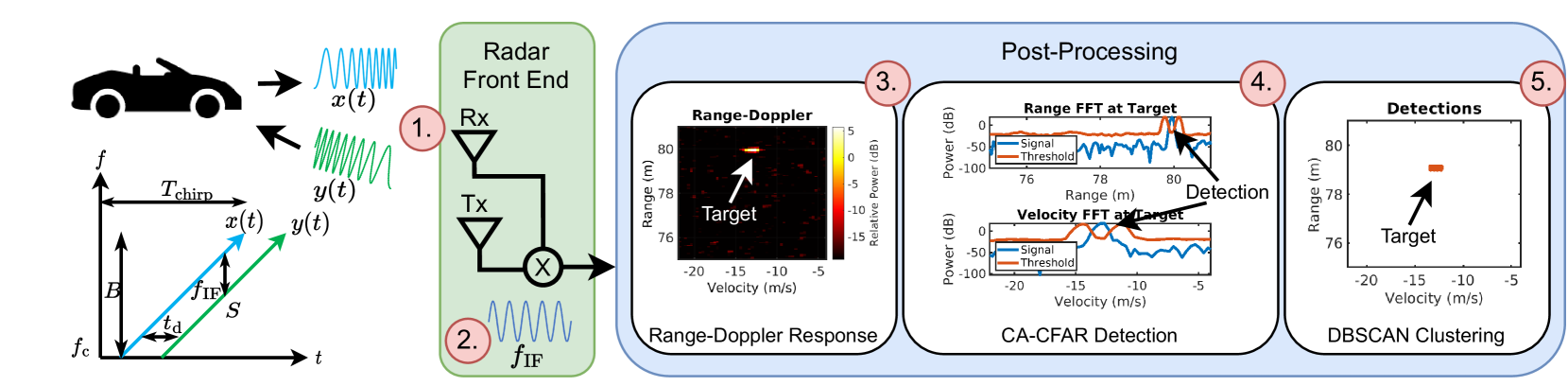
Figure 1: FMCW radar signal processing pipeline.

Step : Transmitter (Tx) and Rx chirps. In each frame, a radar transmits a series of identical “chirps”, whose frequency increases linearly over time. In general, a series of 256 chirps are transmitted per radar frame [26]. Fig. 1 illustrates the frequency response of a single Tx chirp and the corresponding Rx chirp, which is reflected off of an object in the environment and received by the radar. To capture radar parameters, which control sensing performance, we use the following notation: $f_{c}$ denotes the chirp start frequency, $B$ the chirp bandwidth, $T_{\textrm{chirp}}$ is the chirp period, $f_{\textrm{IF}}$ the intermediate frequency (IF) from mixing the Tx chirp with its corresponding Rx chirp, $S$ is the chirp slope, and c denotes the speed of light.

Let $x(t)$ denote the FMCW radar Tx signal corresponding to a single chirp in a radar frame, given by [19, 11, 27, 28]

$$x(t)=e^{j\left(2\pi f_{c}\cdot t+\pi S\cdot t^{2}\right)}.$$ (1)

Consider a target whose relative range and velocity at time $t$ are denoted by $d(t)$ and $v_{\textrm{target}}$, respectfully; thus, $d(t)=R(t)+d_{\textrm{target}}$, where $d_{\textrm{target}}$ is the target’s initial position at the start of the radar frame and $R(t)=\int_{0}^{t}v_{\textrm{target}}\ \textrm{d}t$ is the distance that it has traveled by time $t$ [28, 27].

As the signal propagates at the speed of light (c), the time $t_{\textrm{d}}$ it takes the radar signal to propagate to the target and back is given by $t_{\textrm{d}}=2d(t)/\textrm{c}$. Thus, the reflected signal received by the radar from the target, denoted by $y(t)$, can be captured as

$$y(t)=A_{\textrm{Rx}}\cdot e^{j\left[2\pi f_{c}(t-t_{\textrm{d}})+\pi S(t-t_{\textrm{d}})^{2}\right]}+z(t),$$ (2)

where $A_{\textrm{Rx}}$ and $z(t)$ denote the received signal amplitude and noise, respectively.

Step : Dechirping and IF signal generation. In this step, an IF signal is obtained by mixing the transmitted signal with the received signal; thus, the resulting signal $s_{\textrm{IF}}^{(l)}(t)$ corresponding to the $l$-th chirp is given by

$$s_{\textrm{IF}}^{(l)}(t)=x(t)\cdot y^{*}(t)=A_{\textrm{IF}}\cdot e^{j2\pi f_{\textrm{IF}}\cdot t}\cdot e^{j\phi_{\textrm{doppler}}l}+z^{\prime}(t),$$ (3)

where $f_{\textrm{IF}}:=\frac{2S\cdot d_{\textrm{target}}}{c}$, $\phi_{\textrm{doppler}}:=\frac{4\pi v_{\textrm{target}}\cdot T_{\textrm{chirp}}}{\lambda}$, $\lambda=\textrm{c}/f_{c}$ is the signal wavelength, $A_{\textrm{IF}}$ is the amplitude of the IF signal, and $z^{\prime}(t)=x(t)\cdot z^{*}(t)$ represents the noise present after the mixing  [28, 29] (for details see Appendix -A1).

While the transmitted and received chirp signals may have a bandwidth up to $B=4\thinspace\textrm{GHz}$, modern automotive FMCW radars use a low-pass filter to remove all IF frequencies above 10–20 MHz. For example, the TI IWR1443 mmWave FMCW radar has a maximum IF signal bandwidth of 15 MHz [26]. The maximum IF frequency directly impacts the maximum range that a radar can detect objects at (as we show in (5)), as well as significantly reduces the cost of implementation. Also, as we show in Section IV, this impacts the development of black-box attacks on radar.

Step : Range-Doppler response. The IF frequency, $f_{\textrm{IF}}$, corresponding to a specific target is estimated using a fast Fourier transform (FFT) of the IF signal from (3); then, the target’s range $d_{\textrm{target}}$ is computed using

$$d_{\textrm{target}}=\frac{f_{\textrm{IF}}}{2S}\cdot c.$$ (4)

The range resolution $d_{\textrm{res}}$, defined as the minimum required distance between two targets for a radar to distinguish them, and $d_{\textrm{max}}$, the maximum detection range are defined as [30] (details are provided in Appendix -A2)

$$d_{\textrm{res}}=\frac{\textrm{c}}{2B},\hskip 10.0ptd_{\textrm{max}}=\frac{f_{\textrm{samp}}\cdot\textrm{c}}{B},$$ (5)

where $f_{\textrm{samp}}$ is the radar’s sampling rate of the IF signal.

Multiple chirps in a single frame can be used to detect the velocity of a target, leveraging the slight phase shift, denoted by $\phi_{\textrm{doppler}}$, between chirps due to a target’s relative velocity causing a small change in distance over a chirp’s duration [30]. $\phi_{\textrm{doppler}}$ can be estimated by taking an FFT across all chirps in a frame for each range bin; the resulting FFT will have a peak at $\phi_{\textrm{doppler}}$, and the relative velocity satisfies [30].

$$v=\frac{\phi_{\textrm{doppler}}\cdot\lambda}{4\pi\cdot T_{\textrm{chirp}}}.$$ (6)

In addition, the velocity resolution $v_{\textrm{res}}$ and maximum velocity $v_{\textrm{max}}$ follow (details provided in Appendix -A3)

$$v_{\textrm{res}}=\frac{\lambda}{2N_{\textrm{chirps}}\cdot T_{\textrm{chirp}}},\hskip 10.0ptv_{\textrm{max}}=\frac{\lambda}{4\cdot T_{\textrm{chirp}}},$$ (7)

where $N_{\textrm{chirps}}$ is the number of chirps in a radar frame. The Range-FFT and Doppler-FFT responses are often computed simultaneously using the 2D-FFT operation to generate the Range-Doppler response (as illustrated Fig. 1).

Step : CFAR Detection. Constant false alarm rate (CFAR) detectors are commonly used to detect objects in the Range-Doppler response by estimating the relative noise levels around each Range-Doppler cell. In general, this is non-uniform as different objects in the radar’s field of view may cause more clutter than other objects. Using the estimated noise level at each cell, the CFAR detector computes a threshold configured to achieve a specific probability of false alarm. As the noise level is not constant, the threshold varies to account for the clutter in different regions of the Range-Doppler response.

A cell that has an amplitude above the computed threshold is classified as a detection [31, 32, 33]. Step in Fig. 1 illustrates the computed CFAR detection threshold for the range and velocity domains of a normal target (note that the threshold is not constant). The two most widely used CFAR methods are continuous average CFAR (CA-CFAR) and ordered statistic CFAR (OS-CFAR). The probability of a CA-CFAR detector detecting an object significantly decreases in scenarios with abnormally high clutter in specific regions or with two closely located objects [31, 32]. In this work, we exploit this property to design FN events on systems employing CA-CFAR detectors, as these are more commonly used (e.g., in TI IWR1443 mmWave FMCW radar [26]), but the approach can also be extended to OS-CFAR detectors.

Step : Clustering. The final step of the radar signal processing pipeline is to group the detection cloud points corresponding to the same object using a clustering algorithm. In this work, we focus on the commonly employed density-based spatial clustering of applications with noise (DBSCAN) algorithm [34], which achieves two primary objectives: (i) identifying different targets in the radar’s field of view by grouping together regions with a high density of detection points, and (ii) filtering out detection points corresponding to noise or multi-path reflections (see Step  in Fig. 1).

II-A Non-Adversarial Interference and Interference Mitigation

Even without adversarial activity, radar interference may occur due to the increased proliferation of radar sensing in modern vehicles. FMCW radars are susceptible to three key types of interference: same slope, similar slope, and sweeping interference occurring when an interfering signal has a chirp slope that is the same, similar, or significantly different to the victim radar’s chirp [18, 19]. Generally, interference is the result of multi-path reflections and non-malicious interference from another radar, and all forms of interference can degrade radar performance. Interference could saturate a victim radar’s Rx stage, decrease the signal-to-noise ratio (SNR) of perceived targets, and generate false peaks or ghost targets [21, 22, 23], as well as impact a radar’s Range-Doppler response [21, 22, 23]. resulting in the radar losing a target altogether [19, 20].

Attacks using interference. To the best of our knowledge, no work has considered the effects that a malicious actor could have if they intentionally interfered with a radar using attacks based on carefully-crafted similar slope interference. Existing methods for mitigating (e.g., similar-slope) interference (e.g., [19, 21, 35, 36, 37, 38]) are developed under the assumption that the interference is only sporadic and not adversarial (i.e., malicious). In general most mitigation techniques detect the interference in the time domain of the IF signal and then repair the received signal by nullifying the interference. In this work, we also introduce attacks based on very similar slope interference that result in a FN event for victims employing a CA-CFAR detector. Our attacks are not detectable in the time domain, therefore making such interference mitigation techniques ineffective.

III Attack Objectives and Threat Model

We consider representative attack scenarios illustrated in Fig. 2. Here, we refer to the victim vehicle as the vehicle performing normal radar sensing operations. The attacker’s goal is to produce incorrect sensing outcomes for the victim. The attacker may wish to orchestrate attacks in some relation to an existing target object (e.g., another vehicle) other than the victim, in order to compromise safe victim vehicle operation.

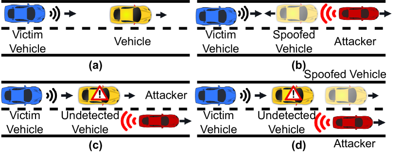
Figure 2: Example traffic scenarios for (a) ao attack, (b) false positive attack, (c) false negative attack, and (d) translation attack (graphics from [39, 40, 41, 42, 43]).

III-A Attack Strategy and Goals

We introduce the false positive (FP), false negative (FN), and translation attacks that use specifically designed signals to add fake targets (FP), remove real targets (FN), or manipulate the range and velocity of existing targets (translation).

FP attack. The first considered attack goal is to cause a FP sensing outcome, where an attacker inserts a spoofed (i.e., ‘fake’) object into the victim radar’s point cloud as illustrated in Fig. 2(b). This is consistent with the existing FP outcomes for camera/LiDAR attacks (e.g., [6, 7, 8, 9]). Intuitively, to achieve this the attacker should send (slightly delayed) chirps identical to that of the victim, emulating the signal reflected from a (spoofed) object. However, unlike attacks on camera and LiDAR where FP attacks only aim to add a spoofed object at a particular range (i.e., distance) from the victim, with radar attacks, the goal is to spoof both an object’s range and velocity. As such, spoofed objects must update their position in consecutive frames based on the desired spoofing velocity; this allows the attack to propagate from perception to the tracking and prediction modules in autonomous vehicles.

FN attack. The second attack goal is to cause a FN sensing outcome, where the victim fails to perceive an existing physical object (Fig. 2(c)). While a FN outcome is hard to achieve with black-box attacks on camera or LiDAR-based sensing, intuitively our approach is to transmit an attacking signal that adds clutter around a desired target, therefore significantly lowering the CA-CFAR detection probability of the object.

Translation attack. The final commonly considered attack goal is to cause a translation event that effectively ‘moves’ a real object from the victim’s point of view (Fig. 2(d)). This is achieved by launching a FN attack to ‘remove’ an actual target while simultaneously employing a FP attack to ‘insert’ a fake object into the victim’s point cloud; as result, the victim fails to detect the real object but detects the fake object.

III-B Environmental Assumptions

We make the following three assumptions:

1. The victim employs the radar processing pipeline from Fig. 1. While we focus on the most commonly employed radar sensing pipeline (e.g., TI IWR1443 mmWave FMCW radar [26]), the presented security analysis and attacks are generalizable to other similar radar designs;

2. We focus on attacking only the victim’s FMCW radar sensor. While most vehicles feature additional sensors (e.g., cameras), our objective is to show that MadRadar’s novel black-box attacks are feasible and effective;

3. We focus on attacking only in the range and velocity domains for the initial black-box attack development. Thus, we assume that the attacker is physically located at the desired angle of attack; e.g., Fig. 2(b) shows the case where the attacker is in front of the victim.

III-C Attacker Capability and Knowledge

We consider physical spoofing attacks, where the attacker can only transmit signals in order to achieve the desired attack outcomes. Unlike existing work, we consider the black-box threat model where the attacker has no knowledge of the radar parameters utilized by the victim. We do assume that the attacker has knowledge about the environment; in particular, the victim’s relative position and velocity for FP attacks so that a spoofed object behaves like a realistic target, as well as the position and velocity of the target object for FN attacks.

IV MadRadar Attack Design

We now present the methodology used to estimate the victim radar’s parameters and show how such estimates can be used to launch FP, FN, and translation attacks. Fig. 3 overviews the design of MadRadar’s black-box attack generator.

IV-A Parameter Estimation

Black-box attacks present a particularly difficult challenge as it is critical that the attacker can accurately estimate, in real-time, the key victim radar parameters. While the architecture from [15] developed a black-box FP attack by estimating a victim’s chirp period ($T_{\textrm{chirp}}$) and chirp slope ($S$), we need to additionally estimate a victim’s frame duration ($T_{\textrm{frame}}$) and predict future frames to develop our novel black-box FN and translation attacks. This presented unique technical challenges as accurate attacks require very precise predictions for when the next victim frame will occur. For example, if the prediction is off by 20 ns, the victim will perceive the spoofed object to be 3 m away from where the attacker intended to add an object. Specifically, the resulting range error satisfies

$$R_{\textrm{error}}=\textrm{c}\cdot t_{\textrm{error}}/2,$$ (8)

where $t_{\textrm{error}}$ is the frame start time prediction error.

We now introduce a real-time sensing module that enables effective FP, FN, and translation attacks by estimating the victim radar’s parameters with low estimation errors; this is performed using three key steps summarized in Fig. 3.

Step 1: Spectrogram generation. Similar to [15], we start by generating a spectrogram for each detected victim frame. The MadRadar prototype runs at 25 MSps sampling rate and checks for victim frames every 0.16 ms. Once a frame is detected by a custom frame detector that tracks increases in received power, we record the received signal for slightly over 2 ms, and then generate a spectrogram that samples the frequency every 2 $\upmu$s[44, 45]. This computation is done in under 10 ms.

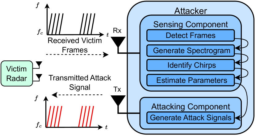
Figure 3: MadRadar block diagram.

Step 2: Identify chirps in spectrograms. While [15] used signal energy over time to estimate the chirp period ($\widetilde{T}_{\textrm{chirp}}$) and the spectrogram of a single chirp to estimate the chirp slope ($\widetilde{S}$), we designed and implemented a peak detection and clustering algorithm to identify the (time, frequency) points corresponding to each chirp within the generated spectrogram. For each chirp’s (time, frequency) points, we use least squares regression to estimate the start time and slope for the $i$-th detected chirp, respectively [46]. The estimates are computed in real-time using the Eigen C++ library [47].

Step 3: Estimate victim parameters. Accurate estimates of the victim radar’s chirp slope ($\widetilde{S}$), chirp period ($\widetilde{T}_{\textrm{chirp}}$), and frame duration ($\widetilde{T}_{\textrm{frame}}$), are achieved by averaging their computed values across multiple recorded victim chirps and frames. While averaging over a large number of computed parameters results in sufficiently accurate estimates for the chirp period and chirp slope, we note that we collect far fewer samples for the frame period (e.g., up to 256 chirps per frame). Thus, we use cross-correlation to compute a more precise frame start time. Specifically, we take the cross-correlation of the first 10 $\upmu$s of the received signal and a computed victim chirp (generated using the estimated parameters) to further improve the accuracy of the estimated frame start time. As shown in our experiments and simulations (Section V), this results in sufficiently accurate estimates after only 6 frames.

In rare cases, the implemented sensing component experiences errors (e.g., classifying one chirp as two different chirps) resulting in significantly incorrect measurements. We account for these erroneous estimates by using the inter-quartile range to identify and filter out outliers [48]. The end result is a robust sensing component capable of quickly and accurately estimating a victim radar’s parameters.

IV-B False Positive Spoofing Attacks

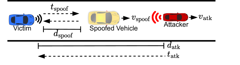
Figure 4: Key attack parameters.

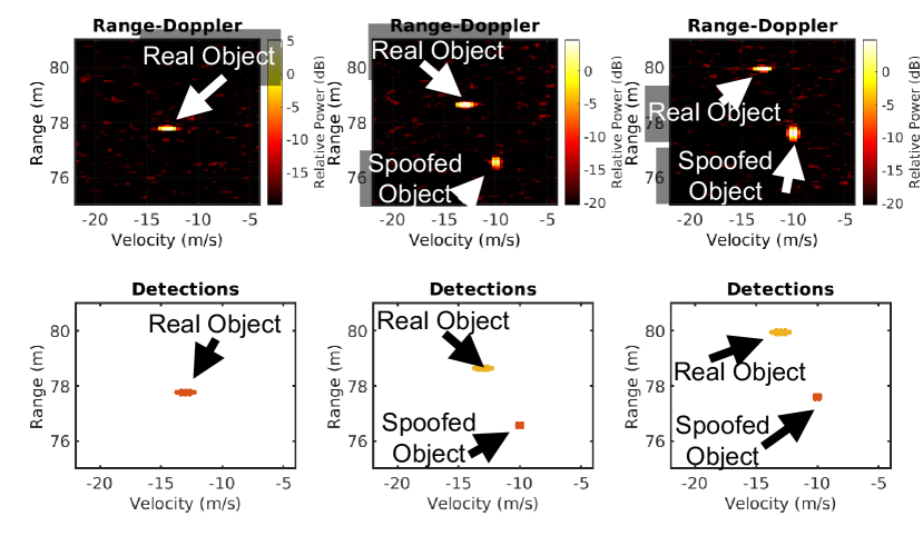
Figure 5: FP attack at frames 1 (no attack), 7, and 10, adding a false moving object in addition to the real moving vehicle. Range-Doppler Plot (Step 3 in Fig. 1) shown in top row; Identified Clusters (Step 5 in Fig. 1) are shown in the bottom row.

Intuitively, the attacker uses the estimated chirp slope ($\widetilde{S}$), chirp period ($\widetilde{T}_{\textrm{chirp}}$), and frame duration ($\widetilde{T}_{\textrm{frame}}$) to launch a FP spoofing attack by transmitting identically sloped radar chirps with a specific delay, $t^{\prime}_{\textrm{d}}$, and phase shift, $\phi^{\prime}_{\textrm{doppler},n}$. Fig. 4 summarizes the key parameters used when constructing the FP attack. Unlike existing white-box FP radar attacks [11, 13], MadRadar’s black-box attack framework does not assume a-priori knowledge of the victim radar’s parameters; it rather uses $t^{\prime}_{\textrm{d}}$ and $\phi^{\prime}_{\textrm{doppler},n}$ based on the desired position and velocity of the spoofed object, respectively, obtained as

$$\begin{split}t^{\prime}_{\textrm{d}}&=t_{\textrm{spoof}}-t_{\textrm{atk}}=\frac{1}{\textrm{c}}\cdot\left(2d_{\textrm{spoof}}-d_{\textrm{atk}}\right),\\ \phi^{\prime}_{\textrm{doppler},n}&=\frac{4\pi}{\lambda}\cdot\left(v_{\textrm{spoof}}-\frac{v_{\textrm{atk}}}{2}\right)\cdot\widetilde{T}_{\textrm{chirp}}\cdot n,\end{split}$$ (9)

where $d_{\textrm{spoof}}$ is the desired spoofing range, $d_{\textrm{atk}}$ is the relative range of the victim w.r.t the attacker, $t_{\textrm{spoof}}$ is the time delay corresponding to a target at $d_{\textrm{spoof}}$, $t_{atk}$ is the propagation delay for a signal to travel $d_{\textrm{atk}}$ from the attacker to the victim, $v_{\textrm{spoof}}$ is the desired spoofing velocity, $v_{\textrm{atk}}$ is the relative velocity of the victim (w.r.t the attacker), and $n$ is the attack chirp index.

Here, we emphasize the importance of accurate estimation of the victim’s position and velocity, which allows for the attacker to spoof objects at specific positions and velocities. We also dynamically scale the amplitude of the Tx signal, denoted by $A_{\textrm{atk}}$, to emulate the propagation loss that scales with $4\pi d_{\textrm{spoof}}^{2}$. Based on (9) and the obtained parameter estimates, the $n$-th chirp of the FP attack signal is computed by

$$x^{(n)}_{\textrm{FP}}(t)=A_{\textrm{atk}}\cdot e^{j\left[2\pi f_{c}(t-t^{\prime}_{\textrm{d}})+\pi\widetilde{S}(t-t^{\prime}_{\textrm{d}})^{2}+\phi^{\prime}_{\textrm{doppler},n}\right]}.$$ (10)

Fig. 5 shows the Range-Doppler response and point cloud over multiple frames for a simulated FP attack. The “real object” in the scene is the attacker while the “spoofed object” is a fake object that the attacker intends to insert. Note that the spoofed object exhibits realistic motion and has a power level expected for objects at that range.

IV-C False Negative Attacks

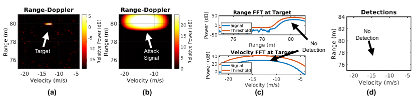
Figure 6: An example of a FN Attack: (a) Range Doppler plot without attack (step 3 in Fig. 1); (b) Range Doppler plot (step 3 in Fig. 1); (c) CFAR threshold (step 4 in Fig. 1); and (d) resulting in no identified clusters (step 5 in Fig. 1).

Intuitively, MadRadar attacks achieve a FN outcome by adding clutter in the Range-Doppler response around a specific target, in order to raise the CA-CFAR detection threshold and thus significantly decrease the probability of the actual target being detected. We start with the FP attack signal from (10) that spoofs a false object at the same range and velocity as an actual target. Next, we slightly smear the spoofed signal in the range domain by using a very similar slope ($\widetilde{S}^{\prime}$) that is slightly offset ($\sim$0.01 MHz/$\upmu$s) from the estimated victim slope ($\widetilde{S}$). This offset is computed to smear the spoofed signal by an additional 1–3 m in the range domain and accounts for the victim radar’s estimated bandwidth, chirp period ($\widetilde{T}_{\textrm{chirp}}$), and chirp slope ($\widetilde{S}$). Finally, the spoofed signal is smeared in the velocity domain by subtly increasing the $\phi^{\prime}_{\textrm{doppler},n}$ phase shift between subsequent chirps; the phase shift for each chirp is

$$\phi^{\prime}_{\textrm{doppler},{n+1}}=\frac{4\pi[(v_{0}+n\cdot\Delta\phi^{\prime})-v_{\textrm{atk}}/2]\widetilde{T}_{\textrm{chirp}}}{\lambda}+\phi^{\prime}_{\textrm{doppler},{n}},$$

where $n$ is the attack chirp index, $\Delta\phi^{\prime}$ is the amount that the $\phi_{doppler}$ increases with each chirp, and $v_{0}$ is a velocity slightly less than $v_{\textrm{spoof}}$ so that the added clutter is centered at $v_{\textrm{spoof}}$.

Thus, the $n$-th chirp of the FN attack signal is given by

$$x^{(n)}_{\textrm{FN}}(t)=A_{\textrm{atk}}\cdot e^{j\left[2\pi f_{c}(t-t^{\prime}_{\textrm{d}})+\pi\widetilde{S}^{\prime}(t-t^{\prime}_{\textrm{d}})^{2}+\phi^{\prime}_{\textrm{doppler},{n}}\right]}.$$ (11)

The resulting attack adds clutter specifically around the target in a way that the CA-CFAR fails to detect the object, as shown in Fig. 6. In particular, the added clutter increases the CFAR threshold in the range and velocity domains at the target location to the point that no object is detected (see Fig. 6(c)).

While the FN attack signal shown in Fig. 6(b) appears easy to identify in the Range-Doppler response, it is unlikely to be detected on current FMCW radars. Most automotive radar systems only utilize CFAR detectors to detect objects in the Range-Doppler response followed by a clustering algorithm to group detections from the CFAR detector. Thus, a real object stays undetected when an attack causes a FN event in the CA-CFAR detector [31, 32, 33]. Additionally, the added clutter is localized around the Range-Doppler bin corresponding to a specific target such that the overall noise level of the entire Range-Doppler response is only slightly raised. Therefore, it is unlikely that our attacks would be detected by additional monitoring of the noise level of the overall Range-Doppler response. Moreover, most existing interference mitigation methods (e.g., [19, 22]) would not be able to detect the attack as the IF signal for the FN attack appears identical to the IF signal from a normal target. Finally, while it would be possible to design an algorithm to detect the added clutter in the Range-Doppler response (e.g., via DNNs), their use would require high computation costs and we are unaware of any such algorithms are currently implemented on commercial systems.

IV-D Translation Attack

The translation attack is achieved by simultaneously transmitting the FP attack from (10) and the FN attack from (11). For the FN attack, we set $d_{\textrm{spoof}}$ and $v_{\textrm{spoof}}$ to the location of an actual target so that it is ’removed’ from the victim radar’s point cloud. For the FP attack, $d_{\textrm{spoof}}$ and $v_{\textrm{spoof}}$ are set to the location where we want the victim to detect the object. The result of the combined FP and FN attack is that an object in the victim radar’s point cloud is ’moved’ as the attacker desires.

V Evaluation of Victim Parameter Estimation

In Section VII, we present a real-time MadRadar physical prototype developed using SDR platforms, but we were limited by the available hardware. Thus, we first employ rigorous simulations to emulate real-world conditions and predict the performance of MadRadar’s framework on a full-scale system. In this section, we present an evaluation of the sensing module before evaluating the full attack performance (Section VI).

V-A Simulation Environment and Setup

We generated realistic environments with multiple objects utilizing the Matlab Phased Array System Toolbox [49]. To start, we used the toolbox’s RadarTarget object to simulate the behavior of radar signals reflecting off of moving targets. Each target’s radar cross-section is randomly selected using a normal distribution with a mean of 15 dBsm and a variance of 5 $\textrm{dBsm}^{2}$, corresponding to the cross-section of a common midsized vehicle [19]. Next, we simulate the effects of range-dependent time delays, propagation losses, phase shifts, and doppler shifts due to signal propagation using the toolbox’s FreeSpace object, where the environment thermal noise level is given by $-174+10\log_{10}B$ (dBm). The Tx’s and Rx’s in our radar and attacker implementations are simulated using objects from the toolbox’s Transmitter and ReceiverPreamp, respectively. Specifically, each Tx has a Tx gain of 36 dB and an output power of 5 dBm without the Tx gain, and each Rx has an Rx gain of 42 dB and a noise figure of 5 dB [50]. Thus, the simulated environment features realistic Tx’s, Rx’s, targets, and signal propagation effects. Finally, we utilize the RangeDopplerResponse and CFARDetector objects from MATLAB’s Phased Array Toolbox and dbscan clustering algorithm from MATLAB’s Machine Learning Toolbox to implement the victim radar signal processing pipeline [51].

Experimental setup. We evaluate the sensing module using the simulated environment with 200 different victim configurations based on realistic parameters of the TI IWR1443 mmWave FMCW radar [26]. Specifically, the victim radar’s chirp slope is sampled uniformly at random from the interval [1 MHz/$\upmu$s, 100 MHz/$\upmu$s], and the chirp period is uniformly sampled from the interval [15 $\upmu$s, 100 $\upmu$s]. To encompass the majority or radar configurations found in the automotive domain, the chirp bandwidth is imposed to be within [30 MHz, 3.5 GHz]. Finally, we set a radar frame rate of 33 Hz, which is the maximum frame rate of an automotive radar  [52, 53]. More details on the test cases can be found in Appendix -B1.

For each victim configuration, 7 victim frames are simulated. We use the estimated victim frame duration ($\widetilde{T}_{\textrm{frame}}$), chirp period ($\widetilde{T}_{\textrm{chirp}}$), and chirp slope ($\widetilde{S}$) at the end of the 7-th frame to assess the parameter estimation accuracy achieved by MadRadar. We also record the predicted frame start time for each victim frame to understand how the estimation accuracy changes with an increased number of detected victim frames. Finally, to evaluate MadRadar’s parameter estimation accuracy regardless of the victim position and velocity, we uniformly sample the attacker’s relative (w.r.t the victim) range ($d_{\textrm{atk}}$) and velocity ($v_{\textrm{atk}}$) at random from the interval [20 m, 100 m] and [$-$10 m/s, 10 m/s].

V-B Simulation Results

We now present the results from our simulated evaluations. We quantify how estimation errors for the victim radar’s parameters lead to spreading and spoofing ($R_{\textrm{error}}$ from (8)) errors. Note that the spoofing velocity is generally unaffected as timing and slope estimation errors almost solely affect the range spoofing performance.

Estimation accuracy for victim chirp slope and period. Figs. 7(a) and 7(b) show the cumulative density function (CDF) of the absolute and relative estimation errors for the victim radar’s chirp period and chirp slope, whose key metrics are summarized in Table I. The results show that 95% of the estimated chirp period values, $\widetilde{T}_{\textrm{chirp}}$, are within 0.59 ns of their actual values, which corresponds to less than 0.1 m of the spoofing error, $R_{\textrm{error}}$, based on (8). Also, 95% of the estimated chirp slope values, $\widetilde{S}$, are within 0.03% of their actual values. While this error could result in some smearing in the range domain, we show in Section VI that this is sufficient enough to launch successful attacks.

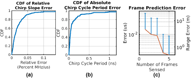
Figure 7: Distributions for parameter estimation errors.

TABLE I: Key parameter estimation error metrics.

Parameter	Error Type	Mean Error	95-th Percentile
Chirp Period	Absolute	0.143 ns	0.586 ns
Chirp Slope	Absolute	0.010 MHz/$\upmu$s	0.0354 MHz/$\upmu$s
Chirp Slope	Relative	$0.025\%$	$0.068\%$

Accuracy vs. Number of measured frames. Fig. 7(c) plots the average absolute error for the predicted frame start times for each of the 200 frames, where the error bars represent the 95-th percentile of the absolute error. The left y-axis reports the prediction error in $\upmu$s while the right y-axis reports the resulting spoofing error in meters using (8). It can be seen that the prediction error decreases as the number of number of considered frames increases. Further, the absolute error significantly decreases after the third victim frame is detected when the sensing component begins using the cross-correlation and the computed victim chirp (from the estimated parameters) to achieve more accurate frame start-time estimates. Overall, in 95% of cases, MadRadar sensing can predict a victim radar’s next frame start time with an accuracy that corresponds to less than 2 m of range spoofing error ($R_{\textrm{error}}$) based on (8).

VI Large Scale Evaluations

The simulation environment introduced in Section V was used for several large-scale evaluations of the accuracy and effectiveness of the MadRadar black-box attack framework. Specifically, we performed 5,000 unique simulations to demonstrate the effectiveness and accuracy of the attacks regardless of the relative range and velocity of the victim. We considered the four victim radar configurations from Table II covering a broad assortment of automotive radar configurations. Note that $d_{\textrm{min}}$ represents the minimum CFAR detection range for each configuration (the full CFAR detection region is provided in Appendix -B3). Here, we start by evaluating spoofing accuracy using configurations C and D, representative of typical automotive long range radar (LRR) and short range radar (SRR), respectively. Then we evaluate how FP and FN attacks effect a victim’s probability of false alarm (PFA) and probability of detection (PD) across all four configurations.

TABLE II: Victim configurations for attack evaluation.

Parameter	(unit)	A	B	C	D
$f_{c}$	GHz	77.0	77.0	77.0	77.0
$B$	MHz	27.81	96.31	1001.51	3935
$S$	MHz/us	1.15	4.04	47.85	187.96
$T_{\textrm{chirp}}$	us	24.11	23.85	20.93	21.63
$N_{\textrm{chirps}}$		128	256	256	256
$d_{\textrm{res}}$	m	7.49	2.14	0.21	0.05
$d_{\textrm{max}}$	m	479	273.93	219.27	223.22
$d_{\textrm{min}}$	m	44.97	19.26	2.14	0.54
$v_{\textrm{res}}$	m/s	0.62	0.31	0.35	0.35
$v_{\textrm{max}}$	m/s	39.49	39.91	45.00	44.99

VI-A Spoofing Accuracy Evaluation

Setup. To evaluate the spoofing accuracy, we consider victim radars with configurations C and D from Table II, representing common real-world configurations. As in Section V, we set the attacker’s relative position uniformly at random from the intervals [20 m, 100 m] and velocity [-10 m/s, 10 m/s] to evaluate performance across varying positions and velocities.

We evaluated the spoofing accuracy for 100 different desired spoofing ranges ($d_{\textrm{spoof}}$) and velocities ($v_{\textrm{spoof}}$), uniformly selected at random from the intervals [50 m, 100 m] and [$-$25 m/s, 25 m/s], respectively; the test case distributions are summarized in Appendix -B2. For each trial, we simulated a total number of 10 radar frames, with the attack starting on the 6th frame. As the first 5 frames were used to sense the victim’s parameters, each trial featured 5 attack frames.

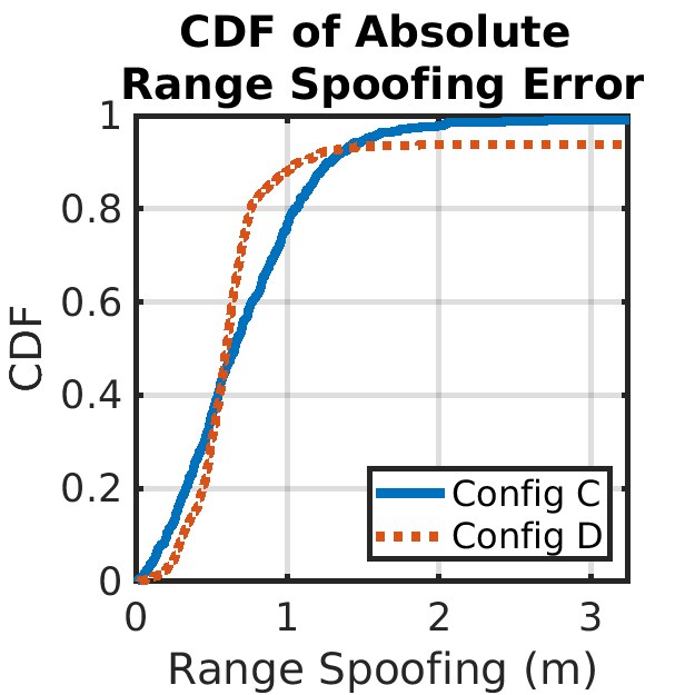
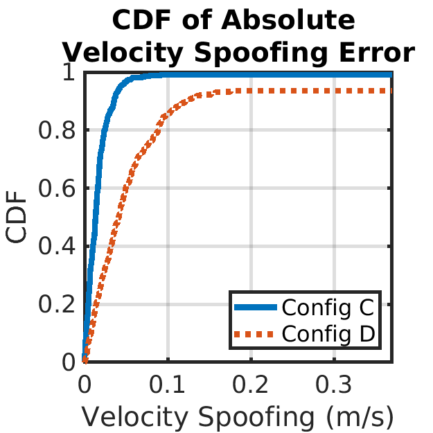
Figure 8: CDFs of absolute error for spoofing accuracy.

TABLE III: Absolute error of attacker spoofing accuracy.

Configuration	Metric	Mean Absolute Error	90th Percentile
C	Range	1.49 m	1.28 m
	Velocity	0.15 m/s	0.04 m/s
D	Range	4.29 m	1.09 m
	Velocity	1.5 m/s	0.12 m/s

Results. Out of the 500 testing frames in the 100 different scenarios, over 90% of the frames resulted in successful, highly accurate attacks. Of the successful attacks, Fig. 8 shows the CDFs for the absolute range and velocity spoofing errors, and the statistics are summarized in Table III. In particular, 90% of the successful attacks had the spoofed range within 1.28 m of the desired range ($d_{\textrm{spoof}}$) and the spoofed velocity within 0.12 m/s of the desired velocity ($v_{\textrm{spoof}}$); the absolute velocity spoofing error is significantly lower than the absolute range spoofing error since the velocity spoofing does not depend on the estimated victim chirp period or the predicted frame start time. Also, the mean absolute error for Config D was relatively high as less than 5% of trials have spoofing errors significantly larger than the rest of the trials. Finally, the remaining inaccurate spoofing attacks resulted from insufficiently accurate victim parameter estimations as discussed in Section V.

VI-B Attack Effectiveness Assessment

Setup. We also evaluated the attack effect on the victim’s PD and PFA, the traditional metrics for assessing radar detection performance. For each configuration in Table II, we performed 400 different simulations for the FP attack, the FN attack, and the base case without attack. Previously, we demonstrated that our framework accurately estimated a victim’s parameters, inserting spoofed signals regardless of the relative position and velocity of the attacker and victim. Now, we show that our attacks are successful regardless of the relative position and velocity of a target-of-interest in the environment.

To maintain a consistent starting point for each simulation, we simulated the attacker 75 m away from the victim with a relative velocity of 2 m/s. When evaluating the effectiveness of our FP attacks on a victim’s PFA, we selected the desired spoofing range and velocity uniformly at random from the intervals [50 m, 100 m] and [$-$25 m/s, 25 m/s], respectively.

For each trial, we simulated an existing target with velocity ($v_{\textrm{target}}$) uniformly chosen at random from the interval [$-$35 m/s, 35 m/s] (35 m/s is roughly 78 mph), and a starting point ($d_{\textrm{target}}$) uniformly selected from the interval [5 m, 143 m]. The radar cross-section of the target in each trial was set using the same method described in Section V-A. For all the trials, we recorded a FN outcome if there was a real target at a specified location but the victim radar did not detect anything within 3$d_{\textrm{res}}$ and 3$v_{\textrm{res}}$ of an target location. We record a FP outcome if the radar detects another object that is not located within 3$d_{\textrm{res}}$ or 3$v_{\textrm{res}}$ of the actual target. Thus, it is possible for both a FP and an FN event to occur in the same trial.

Results. Figs. 9 and 10 show the obtained attack effectiveness; the “Range” axis corresponds to the range of the existing target. To estimate the PD and PFA, we grouped trials into 1 of 30, 5 m range bins, i.e., the first range bin contains the results corresponding to a target within the 0–5 m range.

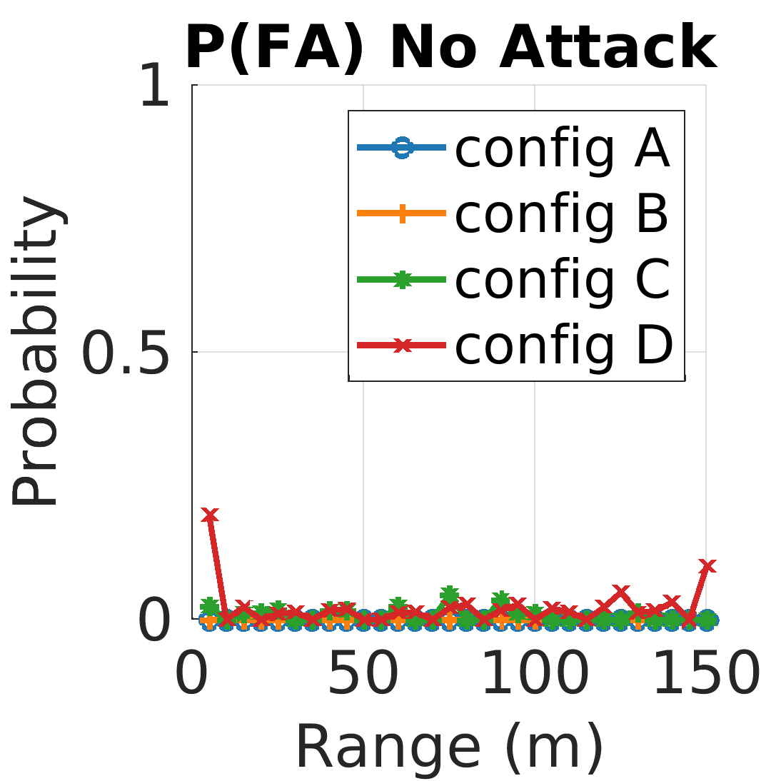
(a) No Attack

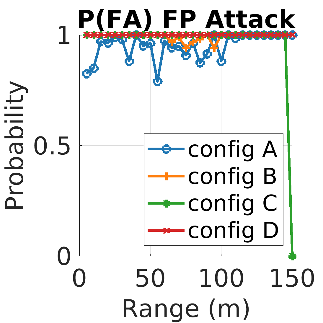
(b) Spoof. FP Attack

Figure 9: Attack effectiveness on probability of false alarm.

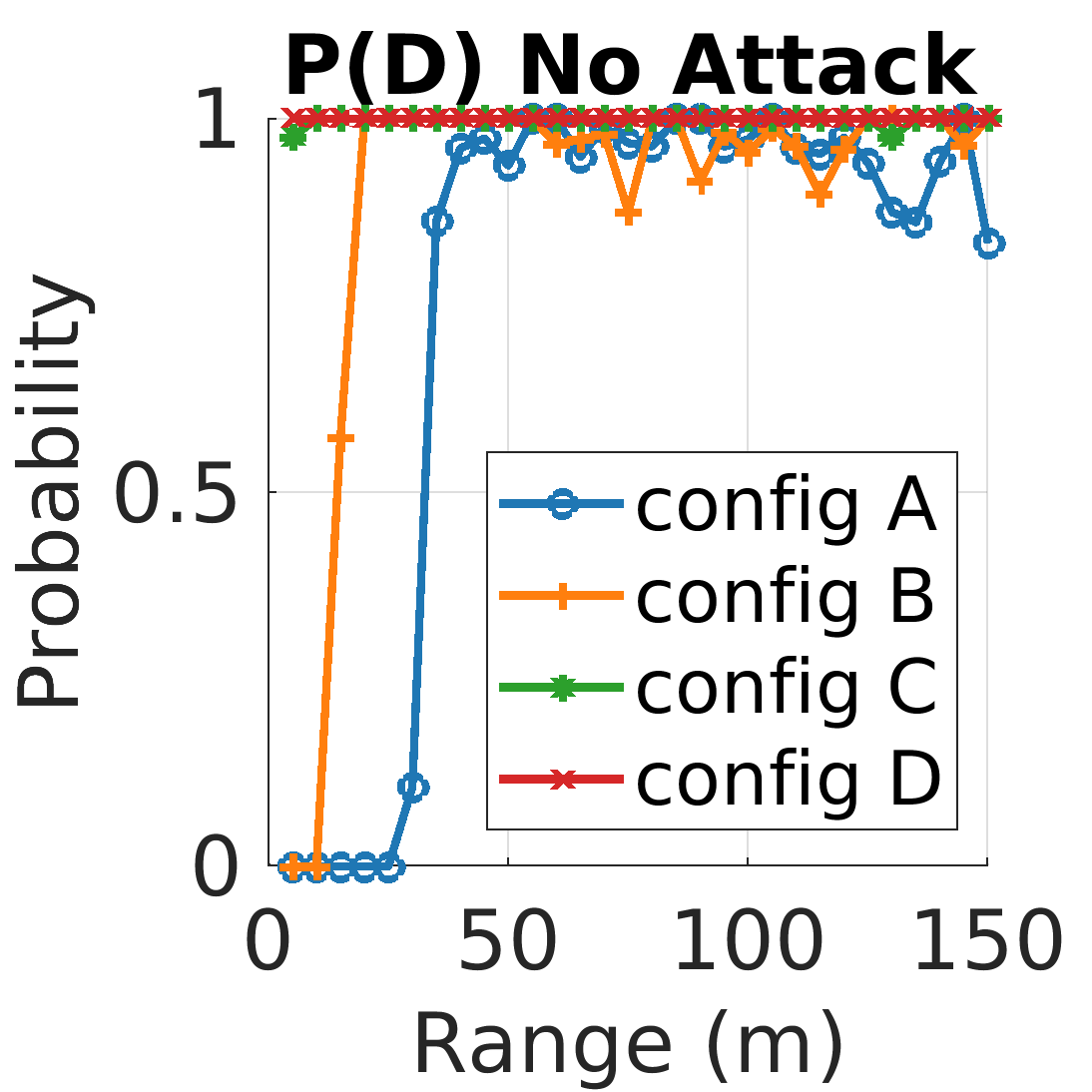
(a) No Attack

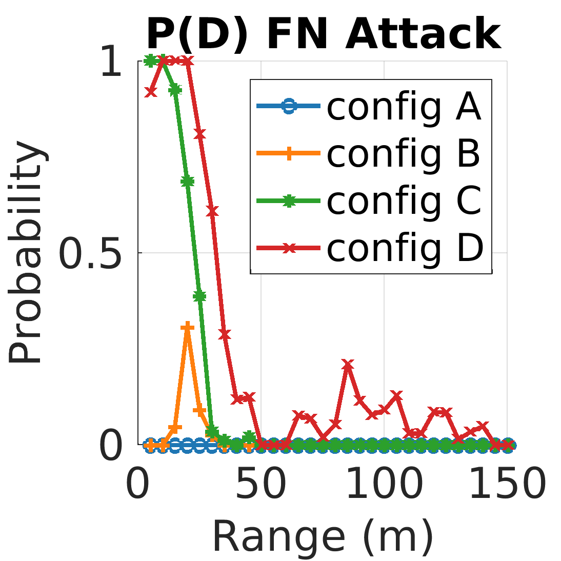
(b) FN Attack

Figure 10: Attack effectiveness on probability of detection.

FP Spoofing Attacks

Fig. 9(a) shows the PFAs for each victim radar configuration without attacks – all have very low PFAs ($<5\%$) in this case. Fig. 9(b) shows the PFAs under the FP spoofing attacks – the PFAs significantly increased, and the attacker was capable of adding a spoofed (i.e., fake) object into the victim radar’s point cloud regardless of the location of the existing (i.e., real) object. This, combined with the results from Fig. 8, shows that FP attacks can successfully insert fake objects very close to the desired locations, no matter the positions of other vehicles in the scene.

FN Attacks

Fig. 10(a) shows the PD for each radar configuration when no attack is present – configurations A and B are unable to detect targets at close ranges due to their poor range resolution ($d_{\textrm{res}}$) and comparatively high CFAR minimum detection range ($d_{\textrm{min}}$) (Table VII in Appendix -B3).

Fig. 10(b) shows the PD for each victim configuration when the FN attack was applied – the attack significantly decreased each radar’s PD, with a steep decline in the victim’s PD for targets roughly 25 m away; the drop at 25 m occurs because it is roughly the point where the power received from the attacker is equal to the power received from the target reflection. While it is expected for PD of a real target to slightly decrease with range (longer ranges experience greater path loss resulting in a reduced SNR), our results show that the FN attacks significantly impact PD compared to operation without an attack. Overall, the results demonstrate that we consistently caused FN events in the victim’s radar.

VII SDR-Based Physical Implementation

We now introduce a real-time prototype implementations of MadRadar and a victim radar using SDR platforms. Additionally, we validate our prototype’s performance on 600 real-world experiments. Section VIII then presents results from multiple real-world case studies.

VII-A Implementation on an SDR Platform

We developed a victim radar and a MadRadar prototype using USRP B210 SDRs, which are controlled by host laptops via the C++-based USRP Hardware Driver (UHD) [24], as illustrated in Fig. 11; the MadRadar prototype alone required 4,500 lines of code. Due to the limitations of available hardware (e.g., the frequency range of [70 MHz, 6 GHz] and maximum sampling rate of 56 MHz for the USRP B210), we consider an operating frequency ($f_{c}$) of 1.5 GHz and a sampling rate of 25 MHz; this corresponds to a victim range resolution ($d_{\textrm{res}}$) of $\sim$6 m and the maximum timing accuracy of the MadRadar attack framework of $\sim$40 ns. We apply longer chirps and frames to achieve a realistic velocity resolution of $\sim$0.8 m/s. While our prototype implementation is constrained by the hardware limitations, it can easily be extended to a full-scale implementation with the use of more capable (and expensive due to high-frequency SDR) hardware platforms.

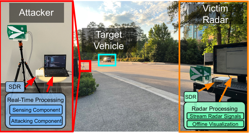
Figure 11: Physical prototype and setup for some case studies.

For our experiments, the victim radar transmits a series of FMCW chirps and records the received signal (i.e., the reflected chirps), which is then processed offline to obtain the Range-Doppler response and detect objects using the pipeline from Fig. 1. The MadRadar prototype, in real-time, estimates the victim radar’s chirp slope ($\widetilde{S}$), chirp period ($\widetilde{T}_{\textrm{chirp}}$), and frame duration ($\widetilde{T}_{\textrm{frame}}$) as described in Section IV. Based on the estimated parameters, the attacker designs and transmits the corresponding signal for launching a FP, FN, or translation attack using (10) and (11). The MadRadar prototype is the first to demonstrate the feasibility of launching real-time black-box FP, FN, and translation attacks on a real-world system.

VII-B Physical Evaluation of Parameter Estimation

Setup. We utilized 500 different victim configurations to validate the MadRadar prototype’s accuracy of estimating the victim radar’s parameter. Due to the hardware limitations, we considered victim configurations with a chirp bandwidth of up to 25 MHz. The victim chirp slope and duration ($S$ and $T_{\textrm{chirp}}$) were chosen uniformly at random from the intervals [0.05 MHz/$\upmu$s, 0.53 MHz/$\upmu$s] and [50 $\upmu$s, 500 $\upmu$s], respectively (details in Appendix -C). The maximum chirp slope was small due to the maximum chirp bandwidth of 25 MHz. For each victim configuration, MadRadar’s sensing module estimates the victim radar’s chirp slope ($\widetilde{S}$), chirp period ($\widetilde{T}_{\textrm{chirp}}$), and frame duration ($\widetilde{T}_{\textrm{frame}}$) over a series of 7 frames. Also, the prototype initiated attacks on the 7-th frame, continuing parameter estimation while performing real-time attacks.

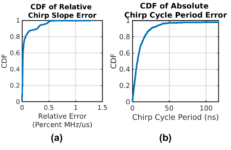
Figure 12: CDFs of the absolute errors for the parameter estimation on SDR-based physical platforms.

TABLE IV: Key parameter estimation error metrics for the implemented physical prototype.

Parameter	Error Type	Mean Error	$95^{th}$ Percentile
Chirp Period	Absolute	18.95 ns	39.09 ns
Chirp Slope	Absolute	0.0025 MHz/$\upmu$s	0.00175 MHz/$\upmu$s
Chirp Slope	Relative	$0.0658\%$	$0.403\%$

Chirp period estimation. Table IV and Fig. 12(a) summarize the results for the chirp period estimation over all physical trials – in 95% of trials, the estimate of the chirp period ($\widetilde{T}_{\textrm{chirp}}$) is within 39.09 ns of the actual chirp period ($T_{\textrm{chirp}}$). Compared with the full-scale simulation-based results from Section V (95% of trials had an absolute error less than 0.59 ns), the timing accuracy decrease by roughly two orders of magnitude is attributed to the described hardware constraints of the prototype system. However, these results indicate that 95% of our chirp period estimates are within one sampling period of the actual victim radar’s chirp period.

Chirp slope estimation. Table IV and Fig. 12(b) summarize the obtained results of physical evaluation – over 95% of the trials result in estimated chirp slope values ($\widetilde{S}$) that are within 0.0017 MHz/$\upmu$s (relative error of 0.403%) of their actual values ($S$). This absolute value is quite low in part because all of the tested radar victim configurations had relatively small slopes. However, the relative value indicates that the accuracy was similar to what was observed in our simulation results (Section V). Again, we attribute the order of magnitude increase in relative slope estimation error to the lower sampling bandwidth of 25 MHz, impacting the maximum achievable resolution when generating a spectrogram of the received signal chirps.

VII-C Physical Evaluation of Spoofing Accuracy

TABLE V: Victim radar configuration used for evaluation of the physical prototype and case studies

Parameter	(Units)	Experimental Configuration
$f_{c}$	GHz	1.5
$B$	MHz	25.00
$S$	MHz/us	0.05
$T_{\textrm{chirp}}$	us	501.12
$N_{\textrm{chirps}}$		256
$d_{\textrm{res}}$	m	6.09
$d_{\textrm{max}}$	m	1,558.92
$d_{\textrm{min}}$	m	24.35
$v_{\textrm{res}}$	m/s	0.78
$v_{\textrm{max}}$	m/s	99.71

Setup. We evaluate spoofing accuracy over 100 unique trials where each real-time trial involved 15 attacking frames. Table V summarizes the victim configuration used for all trials; this configuration used a longer chirp duration ($T_{\textrm{chirp}}$) to achieve more realistic velocity resolution ($v_{\textrm{res}}$) given the lower operating frequency ($f_{c}$) of the physical prototype. The spoofing range ($d_{\textrm{spoof}}$) and velocity ($v_{\textrm{spoof}}$) for each trial was uniformly chosen at random from the interval [60 m, 200 m] and [-25 m/s, 25 m/s] (see Appendix -C for distribution).

TABLE VI: Absolute error of the attack spoofing accuracy.

Metric	Mean Absolute Error	90th Percentile
Range	7.53 m	9.67 m
Velocity	1.42 m/s	1.80 m/s

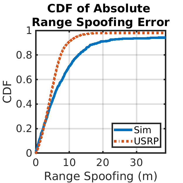
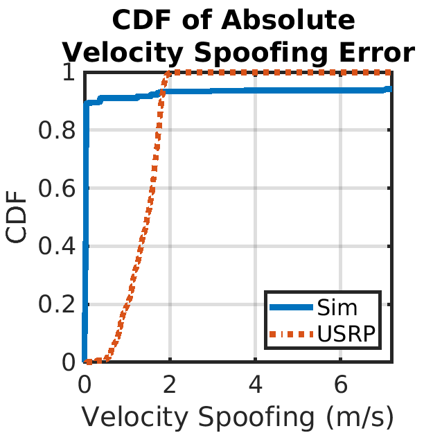
Figure 13: CDFs of absolute error of spoofing accuracy obtained in physical experiments (orange) and corresponding simulation (blue).

Results. Fig. 13 reports the obtained CDFs for the absolute range and velocity errors, whereas Table VI summarizes the relevant statistics – 90% of trials had the obtained range within 9.67 m of the desired spoofing range ($d_{\textrm{spoof}}$) and the obtained velocity 1.80 m/s of the desired spoofing velocity ($v_{\textrm{spoof}}$). To compare the experimental results with the simulation-based results presented in Section VI, we simulated the exact same set of physical scenarios using the simulated environment from Section V. In Fig. 13, the simulated results appear in blue while the results obtained in physical experiments appear in orange. We highlight how our prototype spoofed an object’s range slightly more accurately than our simulation predicted. While we observe that the prototype’s velocity spoofing was less accurate than the simulations predicted, we attribute this discrepancy to the phase noise in the USRP B210, which our simulations do not account for.

In summary, the results from our real-world physical experiments demonstrate that MadRadar estimates a victim’s parameters and inserts spoofed objects with the anticipated level of accuracy given the hardware limitations.

VIII Real World Case Studies

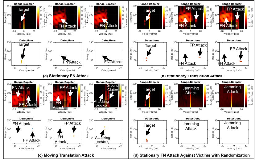
Figure 14: Attack progressions for real world case studies.

We now demonstrate the real-world capability of MadRadar through several real-world case studies. We start by demonstrating FN and translation attacks against stationary victims followed by a demonstration of a translation attack on a moving victim. To the best of our knowledge, this it the first work to demonstrate each of the following attack capabilities in realistic case studies. Results and details from these and additional case studies, including time-synchronized videos, are available on the project website [25].

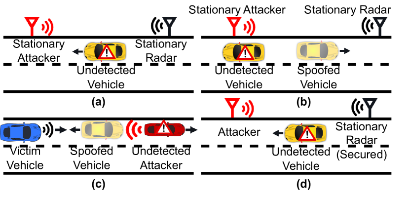
Figure 15: Considered case study threat scenarios for (a) stationary FN attack, (b) stationary translation attack, (c) moving translation attack, and (d) stationary ’Jamming’ attack.

VIII-A Stationary Case Studies

We first present case studies where a stationary attacker is set up to attack a stationary victim trying to detect objects on the road. Meanwhile, the attacker estimates the victim radar’s parameters in real-time and then simultaneously launches the MadRadar attacks. This experimental setup is commonly found in the real world including infrastructure sensors detecting vehicles at stoplights and stopped vehicles sensing oncoming traffic prior to pulling out of a parking lot.

Setup. Fig.11 illustrates the experimental setup while Fig. 15(a) and Fig. 15(b) portray the threat scenarios used for the stationary case studies. Here, the attacker and victim were placed 15 m apart from each other. A real target vehicle then drove away from the victim at approximately 9 m/s ($\sim$20 mph). Finally, the victim radar employed the configuration described in Table V.

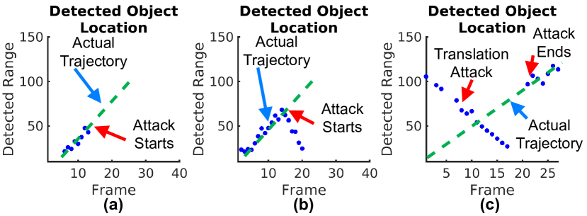
Figure 16: Radar detections over time for: (a) stationary FN attack; (b) stationary translation attack; and (c) moving translation attack.

FN attacks. We launched FN attacks with $d_{\textrm{spoof}}$ and $v_{\textrm{spoof}}$ set to 75 m and -5 m/s, respectively. The attack started on the $\textrm{11}^{\textrm{th}}$ sensed frame; this coincided with causing a FN event when the target vehicle was at 50 m distance. The attack progression is shown in Fig. 14(a) while Fig. 16(a) shows the detected target location for each victim radar frame. The first column of Fig. 14(a) presents the victim’s perception prior to the attack while the second and third columns present the victim’s perception while under attack. The victim radar’s immediately fails to detect the target vehicle once the FN attack is launched. Such a result is incredibly critical as the attack has effectively ‘removed’ an object from the victim’s point cloud/scene.

Translation attack. Here, we simultaneously launched the FN attack from (11) and FP attack from (10). The FN attack was launched with $d_{\textrm{spoof}}$ and $v_{\textrm{spoof}}$ set to 75 m and -5 m/s, respectively. Simultaneously, the FP attack started at 75 m while propagating towards the victim with a velocity of 10 m/s. The attack progression is featured in Fig.14(b) while Fig. 16(b) presents the attack detections over time. The first column of Fig. 14(b) presents the victim’s perception prior to the attack while the second and third columns present the victim’s perception while under attack. Even though the actual target of interest was moving away from the victim for the duration of the experiment, we observe that the victim erroneously perceived that the target vehicle started moving toward it once the attack started. Also, note that the power level of the spoofed (fake) object increases as it gets ‘closer’ to the victim radar. Overall, such an attack is incredibly powerful as an attacker can effectively ‘move’ any specific object in the victim radar’s point cloud (i.e., perceived scene).

VIII-B Moving Case Studies

We now demonstrate that MadRadar can launch succesful black-box translation attacks from a moving vehicle, which can critically affect safety of autonomous vehicles.

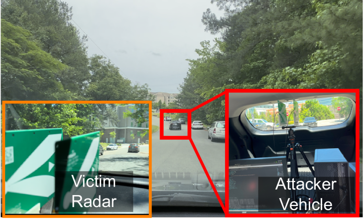
Figure 17: Experimental setup for the moving vehicles studies.

Setup. Fig. 17 and Fig. 15(c) feature the experimental setup and threat scenarios considered in our moving-vehicle case studies. The MadRadar platform was placed in the trunk of the attack vehicle so that it could sense the victim radar’s parameters and launch attacks. The victim radar was placed in a separate vehicle that moved independently from the attacker’s vehicle.

At the start of the experiment, the attacker and victim began driving forward at 13 m/s and 4.5 m/s (30 mph and 10 mph), respectively. Here, the attacker immediately launched the translation attack – the FN attack started at a target range of 75 m and propagated away from the victim radar with the target’s velocity of $\sim$10 m/s, while the FP attack started at 100 m and propagated towards the victim radar with velocity of 12 m/s.

Results. The attack progression is featured in Fig. 14(c) while Fig. 16(c) reports the detected target locations over time. The first and second columns of Fig. 14(c) presents the victim radar’s perception during the translation attack while the third column presents its perception after the translation attack concluded. The successfully launched translation attack lead the victim to believe that the attack vehicle was moving towards it even though the attack vehicle was actually moving away from it. Such an attack is incredibly powerful as the victim failed to detect the attacker’s actual location while simultaneously detecting the attacker’s fake location; this could lead to very dangerous situations in real-world scenarios. Finally, the victim was only able to detect the actual location of the attacker once the translation attack completes, further demonstrating the effectiveness of the attack.

IX Discussion and Future Work

IX-A Limitations of MadRadar

Angle of Arrival (AoA). Modern radars detect an object’s range, velocity, and angle of arrival. As dicussed in Section III, we assume that the attacker is physically located at the desired angle of attack. More versatile attackers would attack a victim from any angle within the victim’s field of view. Future works will explore methods for angular spoofing attacks.

CFAR detection. In this work, we focused MadRadar attacks on radars employing the widely-used CA-CFAR detector. However, other CFAR detectors exist, e.g., OS-CFAR [31, 32, 33]. While we expect that the presented FN and translation attacks can be used for other radar designs, future work will include attack demonstrations against other CFAR detectors.

Physical implementation. As described in Section VII, our physical prototype was limited by the available hardware. A more capable (yet, very expensive) hardware platform could be used to implement a full-scale version. To start, an RF chain capable of converting between baseband frequencies and mmWave frequencies (77–81 GHz) could be used, but at such high frequencies, with the cost of tens of thousands of dollars. Moreover, generating a spectrogram for the full 4 GHz bandwidth utilized by automotive radars would require an expensive RFSOC board supporting complex sampling rates of at least 4 Gsps (such platforms have been used in e.g., [55]). Future works will seek to develop a full scale system.

IX-B Potential Defenses and Future Works

Parameter randomization. Most PHY attacks on automotive FMCW radars, including ours, rely on the ability to predict when the victim’s next frame will occur. As described in [18, 21, 35, 11], a defense against such attacks could be introducing small random changes to a radar’s chirp period ($T_{\textrm{chirp}}$), chirp slope ($S$), and frame duration($T_{\textrm{frame}}$) at each frame; no commercially available mmWave radars support this. While such a defense could thwart most other spoofing attacks, MadRadar framework can be easily modified to launch effective attacks against victims employing such a defense.

Using the same stationary experimental setup from Section VIII, we modified our victim to randomize the start time of each frame using a normally distributed offset with a mean of 0 $\upmu$s and $3\sigma$ (3$\times$ standard-deviation) of 3 $\upmu$s. We modified the MadRadar prototype to detect victims employing parameter randomization using the Liklihood Ratio Test [56]. Once the attacker detects parameter randomization, it generates an optimal FN attack against randomization (i.e., FN ‘jamming’ attack) leveraging the FN attack from (11) to cover a much larger range ($\sim$1,000 m) and velocity ($\sim$200 m/s) spread.

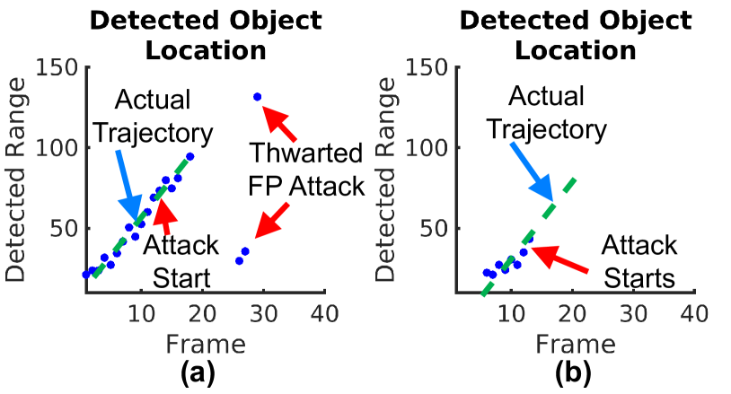
Figure 18: Detections over time for attacks: (a) without randomization detection; and (b) with randomization detection.

The first column of Fig. 14(d) features the victim’s perception when not under attack, whereas the 2nd and 3rd columns present its perception under the optimal FN ‘jamming’ attack. Fig. 18 compares the victim’s detections over time when attacked by our standard translation attack and our optimal FN ‘jamming’ attack. We highlight how the optimized FN ‘jamming’ attack still prevents the victim from detecting the target even though standard spoofing attacks may be thwarted in a sense that the accuracy of the FP detections is significantly affected. As an avenue for future work additional analysis of defense mechanisms against MadRadar will be performed.

Multi-sensor fusion. While we focus on attacking a single radar sensor, modern vehicles utilize signals from multiple sensors including cameras, LiDARs, and radars. Even if our attack was successful in manipulating a victim radar’s data, it is possible that the attack could be thwarted using the victim’s other sensors. Still, such a defense is not guaranteed to succeed as works such as [8] demonstrated successful attacks against victims employing LiDAR-camera sensor fusion. Future works will investigate PHY radar attacks on vehicles employing radar-camera and radar-LiDAR-camera sensor fusion.

X Conclusion

In this work, we presented the design of MadRadar, a novel black-box physical layer attack framework for mmWave FMCW automotive radars. Unlike previous works that focused solely on ‘adding’ fake objects into a victim radar’s point cloud, this is the first work to introduce the false-negative and translation attacks that effectively ‘remove’ or ‘move’ detections of existing objects in the victim radar’s point cloud. Further, all but one of the previous (false-positive only) spoofing attacks assumed prior knowledge of the victim radar’s parameters. By comparison, MadRadar estimates the victim’s chirp period, chirp slope, and frame duration with sufficient accuracy to implement successful attacks over 95% of the time. We have experimentally validated the feasibility and effectiveness of the proposed attacks by developing a real-time MadRadar prototype using SDR platforms. Finally, we have demonstrated the real-world capabilities of MadRadarthrough real-world case studies.

-A FMCW Radar Signal Processing Theory

-A1 Simplification of the IF Signal

As discussed in (3) from Section II, the IF signal is obtained by mixing the transmitted signal with the received signal – i.e.,

$$\begin{split}s_{\textrm{IF}}^{(l)}(t)=&x(t)\cdot y^{*}(t)\\ =&A_{\textrm{Rx}}\cdot\exp\{j\left[2\pi f_{c}\cdot t+\pi S\cdot t^{2}\right]-\\ &\hskip 2.84544ptj\left[2\pi f_{c}(t-t_{\textrm{d}})+\pi S(t-t_{\textrm{d}})^{2}\right]\}+z^{\prime}(t)\\ =&A_{\textrm{Rx}}\cdot\exp\{j[2\pi f_{c}\cdot t+\pi S\cdot t^{2}-2\pi f_{c}\cdot t+\\ &\hskip 2.84544pt2\pi f_{c}\cdot t_{\textrm{d}}-\pi S(t^{2}-2t\cdot t_{\textrm{d}}+t_{\textrm{d}}^{2})]\}+z^{\prime}(t)\\ =&A_{\textrm{Rx}}\cdot\exp\{j[2\pi S\cdot t_{\textrm{d}}\cdot t+2\pi f_{c}\cdot t_{\textrm{d}}-\\ &\hskip 2.84544pt\pi S\cdot t_{\textrm{d}}^{2}]\}+z^{\prime}(t),\end{split}$$ (12)

where $z^{\prime}(t)=x(t)z^{*}(t)$ represents the noise present after the mixing. From (12), several simplifications can be made. First, $2\pi S\cdot t_{\textrm{d}}\cdot t$ can be simplified by recognizing that $R(t)<<d_{\textrm{target}}$ and defining $f_{\textrm{IF}}$ as

$$f_{\textrm{IF}}:=\frac{2S\cdot d_{\textrm{target}}}{\textrm{c}}.$$ (13)

The simplified term can then be expressed as

$$\begin{split}2\pi S\cdot t_{\textrm{d}}\cdot t&=2\pi S\left(\frac{2(R(t)+d_{\textrm{target}})}{\textrm{c}}\right)t,\\ &\approx 2\pi\frac{2S\cdot d_{\textrm{target}}}{\textrm{c}}t,\\ &=2\pi f_{IF}\cdot t.\end{split}$$ (14)

Next, $2\pi f_{\textrm{c}}\cdot t_{\textrm{d}}$ can be simplified by sampling $R(t)$ at each chrip using $R(l\cdot T_{\textrm{chirp}})=v_{\textrm{target}}\cdot l\cdot T_{\textrm{chirp}}$ where $l$ is the chirp number in the frame. Additional we define $\phi_{\textrm{doppler}}$ as

$$\phi_{\textrm{doppler}}=\frac{4\pi v_{\textrm{target}}\cdot T_{\textrm{chirp}}}{\lambda}.$$ (15)

Using these simplifications, $2\pi f_{c}\cdot t_{\textrm{d}}$ simplifies as follows:

$$\begin{split}2\pi f_{c}\cdot t_{\textrm{d}}=&2\pi f_{c}\frac{2(R(l\cdot T_{\textrm{chirp}})+d_{\textrm{target}})}{\textrm{c}}\\ =&\frac{4\pi(R(l\cdot T_{\textrm{chirp}})+d_{\textrm{target}})}{\lambda}\\ =&\frac{4\pi R(l\cdot T_{\textrm{chirp}})}{\lambda}+\frac{4\pi d_{\textrm{target}}}{\lambda}\\ =&\frac{4\pi v_{\textrm{target}}\cdot l\cdot T_{\textrm{chirp}}}{\lambda}+\frac{4\pi d_{\textrm{target}}}{\lambda}\\ &=\phi_{\textrm{doppler}}\cdot l+\frac{4\pi d_{\textrm{target}}}{\lambda}.\end{split}$$ (16)

Finally, $\pi S\cdot t_{\textrm{d}}^{2}$ can be simplified by recognizing that $R(t)^{2}<<2R(t)d_{\textrm{target}}<<d_{\textrm{target}}^{2}$. The simplified term can then be expressed as

$$\begin{split}\pi S\cdot t_{\textrm{d}}^{2}=&\pi S\left(\frac{2(R(t)+d_{\textrm{target}})}{\textrm{c}}\right)^{2}\\ =&\pi S\frac{4}{\textrm{c}^{2}}(R(t)^{2}+2R(t)d_{\textrm{target}}+d_{\textrm{target}}^{2})\\ \approx&\frac{4\pi S\cdot d_{\textrm{target}}^{2}}{\textrm{c}^{2}}.\end{split}$$ (17)

Applying (14),(16), and (17) to (12) gives

$$\begin{split}s_{IF}^{(l)}(t)=&A_{RX}\cdot\exp\{j[2\pi f_{IF}\cdot t+\phi_{\textrm{doppler}}l+\\ &\frac{4\pi d_{\textrm{target}}}{\lambda}-\frac{4\pi S\cdot d_{\textrm{target}}^{2}}{\textrm{c}^{2}}\}+z^{\prime}(t).\end{split}$$ (18)

where $s_{IF}^{(l)}(t)$ is the IF signal corresponding to the $l$th chirp. Finally, by simplifying and defining $A_{IF}=A_{Rx}\cdot\exp\left\{j\left[\frac{4\pi d_{\textrm{target}}}{\lambda}-\frac{4\pi S\cdot d_{\textrm{target}}^{2}}{\textrm{c}^{2}}\right]\right\}$, (18) can be rewritten in terms of a range, velocity (Doppler), and noise term as

$$\begin{split}s_{IF}^{(l)}(t)=&\\ &A_{IF}\cdot\exp(j2\pi f_{IF}\cdot t)\cdot\exp(j\phi_{\textrm{doppler}}l)+z^{\prime}(t).\end{split}$$ (19)

-A2 Range Resolution and Maximum Range

The output of an FFT (in particular, the dominant signal frequencies) of the signal from (3) is used to evaluate the IF frequency. Thus, the resolution of the FFT also limits the range resolution and maximum range that a radar can detect a target at. By definition, an FFT can separate two tones if they have a frequency difference greater than $\frac{1}{T}$ where $T$ is the observation period. As such, two targets can be separately identified as long as their IF frequencies are greater than $T_{\textrm{chirp}}$ [30].

Therefore, by converting from IF frequency to distance provides us with the following range resolution

$$\begin{split}\Delta f_{IF}=&\frac{2\Delta d\cdot S}{\textrm{c}}=\frac{2\Delta d\cdot B}{\textrm{c}\cdot T_{\textrm{chirp}}}\geq\frac{1}{T_{\textrm{chirp}}}\\ \Rightarrow&\Delta d\geq\frac{\textrm{c}}{2\cdot B}\Rightarrow d_{\textrm{res}}=\frac{\textrm{c}}{2\cdot B}.\end{split}$$ (20)

On the other hand, the maximum range that a radar could detect is limited by the IF frequency bandwidth, which is also based on the ADC sampling rate used to record the IF signal [30]. Hence, the maximum range that a radar can detect an object at is obtained as

$$\begin{split}f_{\textrm{samp}}\geq&f_{\textrm{IFMax}}=\frac{2S\cdot d_{\textrm{max}}}{\textrm{c}}\Rightarrow d_{\textrm{max}}=\frac{f_{\textrm{samp}}\cdot\textrm{c}}{S}.\end{split}$$ (21)

-A3 Velocity Resolution and Maximum Velocity

First, we observe that the phase shift caused by an object’s velocity must not be greater than $\pi$ between successive chirps so as not to be ambiguous. Thus, the maximum velocity satisfies satisfies [30]

$$\phi_{\textrm{doppler}}\leq\pi\hskip 10.0pt\Rightarrow\hskip 10.0ptv\leq\frac{\lambda}{4T_{\textrm{chirp}}}.$$ (22)

A similar approach can be used to determine the velocity resolution. In radians, two tones are separable if $\Delta\phi_{\textrm{doppler}}\geq\frac{2\pi}{N_{\textrm{chirps}}}$, where $N_{\textrm{chirps}}$ is the number of chirps. Hence, the velocity resolution satisfies [30]

$$\begin{split}\phi_{\textrm{doppler}}&=\frac{4\pi v_{\textrm{target}}\cdot T_{\textrm{chirp}}}{\lambda},\\ \Delta\phi_{\textrm{doppler}}&\geq\frac{2\pi}{N_{\textrm{chirps}}}\hskip 10.0pt\Rightarrow\hskip 10.0pt\Delta v\geq\frac{\lambda}{2N_{\textrm{chirps}}T_{\textrm{chirp}}},\end{split}$$ (23)

where $N_{\textrm{chirps}}$ is the number of chirps in a radar frame.

-B Simulation Details

-B1 Distribution of Test Cases for Simulated Victim Radar Parameter Estimation

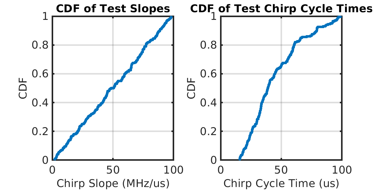
Figure 19: Test case distribution for the simulation-based evaluation of the victim radar parameter estimation.

Fig. 19 shows the distribution of chirp periods and chirp slopes used for the simulation-based evaluation of the victim parameter sensing presented in Section V.

-B2 Distribution of Test Cases for Attacker Spoofing Accuracy

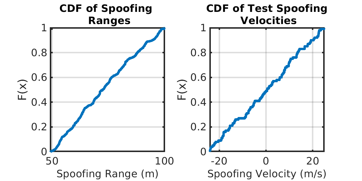
Figure 20: Test case distribution for the simulation-based spoofing accuracy evaluation.

The distributions of the desired spoofing ranges ($d_{\textrm{spoof}}$) and velocities ($v_{\textrm{spoof}}$) used for the simulation-based evaluation of the attack spoofing accuracy in Section VI are presented in Fig. 20.

-B3 CFAR Detection Regions for Large-Scale Evaluation

The CFAR detection regions for each victim radar configuration utilized in the simulation-based large scale evaluations from Section VI, are listed in Table VII.

TABLE VII: CFAR detection regions for considered victim configurations

Configuration	Range Region (m)	Velocity Region (m/s)
A	44.97 to 427.18	-33.94 to 34.55
B	19.26 to 252.53	-35.23 to 35.54
C	2.14 to 216.91	-39.73 to 40.075
D	0.54 to 222.62	–39.72 to 40.073

-C Details for Test Cases Used for Physical Evaluation

-C1 Distribution of Test Cases for Physical Evaluation of the MadRadar Sensing Accuracy

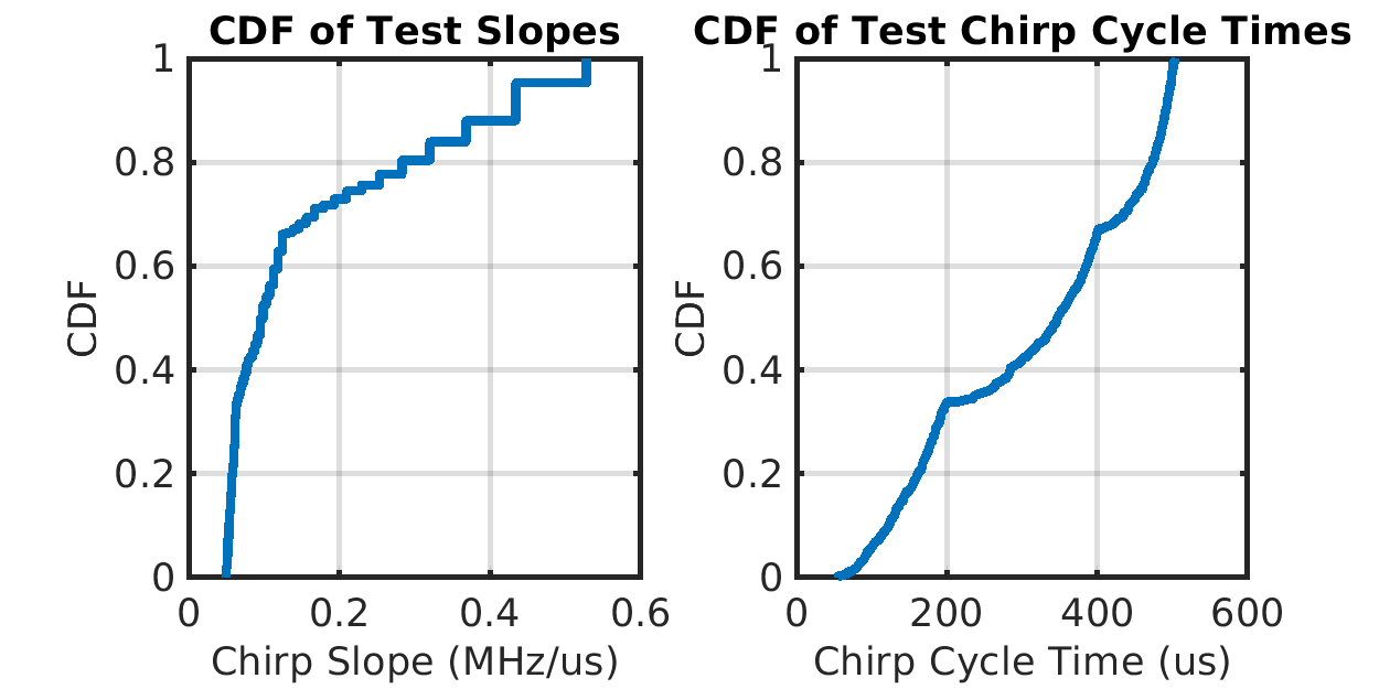
Figure 21: Distribution of test case used for experimental evaluation of the accuracy of victim radar parameter estimation.

Fig. 21 presents the distributions of the desired victim radar chirp periods ($T_{\textrm{chirp}}$) and chirp slopes ($S$) used for the experimental evaluations performed in Section VII. To generate samples at various chirp cycle times and chirp slopes, we performed 200 trials for each of the following three groups: chirps with periods in the range [50 $\upmu$s, 200 $\upmu$s], chirps with periods in the range [200 $\upmu$s, 400 $\upmu$s], and chirps with periods in the range [400 $\upmu$s, 500 $\upmu$s]. This was done to validate our real-time experimental sensing component using a wide range of victim configurations, and it explains the three distinct groupings that appear in the distribution.

-C2 Distribution of test cases used for physical evaluation of the attack spoofing accuracy.

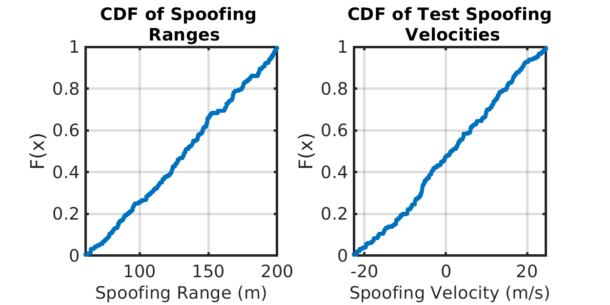
Figure 22: Distributions of test cases used for experimental evaluation of MadRadar spoofing accuracy.

Fig. 22 presents the distribution of the desired spoofing ranges ($d_{\textrm{spoof}}$) and velocities ($v_{\textrm{spoof}}$) used to experimentally evaluate the spoofing accuracy of the MadRadar prototype framework in Section VII.

References

- [1] Anonymous, “How Millimeter Wave Automotive Radar Enhances Advanced Driver Assistance Systems (ADAS) and Autonomous Driving,” Keysight Technologies, Tech. Rep., 2020. [Online]. Available: https://www.keysight.com/us/en/assets/7018-06176/white-papers/5992-3004.pdf
- [2] A. Benjamin, “Imaging radar: one sensor to rule them all,” Texas Instruments, Tech. Rep., 2019. [Online]. Available: https://e2e.ti.com/blogs_/b/behind_the_wheel/posts/imaging-radar-using-ti-mmwave-sensors
- [3] M. Gardill, “Automotive Radar - An Overview on State-of-the-Art Technology,” 2019. [Online]. Available: https://www.youtube.com/watch?v=P-C6_4ceY64&ab_channel=IEEEMicrowaveTheoryandTechnologySociety
- [4] K. Ramasubramanian, K. Ramaiah, and A. Aginskiy, “Moving from Legacy 24 GHz to State-of-the-Art 77-GHz Radar,” Texas Instruments, Tech. Rep., 2017. [Online]. Available: https://www.ti.com/lit/wp/spry312/spry312.pdf
- [5] Anonymous, “Radar & LiDAR Autonomous Driving Sensors by Mobileye & Intel,” Mobileye, Tech. Rep., 2022. [Online]. Available: https://static.mobileye.com/website/corporate/media/radar-lidar-fact-sheet.pdf
- [6] J. Sun, Y. Cao, Q. A. Chen, and Z. M. Mao, “Towards Robust LiDAR-based Perception in Autonomous Driving: General Black-box Adversarial Sensor Attack and Countermeasures,” in USENIX Secur. Simp. (USINEX Security’20), 2020, pp. 877–894.
- [7] M. Abdelfattah, K. Yuan, Z. J. Wang, and R. Ward, “Adversarial Attacks on Camera-LiDAR Models for 3D Car Detection,” in 2021 IEEE/RSJ Int. Conf. Intell. Robots and Syst. (IEEE IROS’21). Prague, Czech Republic: IEEE, sep 2021, pp. 2189–2194.
- [8] R. S. Hallyburton, Y. Liu, Y. Cao, M. Pajic, and Z. M. Mao, “Security Analysis of Camera-LiDAR Fusion Against Black-Box Attacks on Autonomous Vehicles,” in 31st USENIX Secur. Symp. (USENIX Security’22), 2022, pp. 1903–1920.
- [9] Y. Cao, C. Xiao, B. Cyr, Y. Zhou, W. Park, S. Rampazzi, Q. A. Chen, K. Fu, and Z. M. Mao, “Adversarial Sensor Attack on LiDAR-based Perception in Autonomous Driving,” in Proc. 2019 ACM SIGSAC Conf. Comput. and Commun. Secur. (ACM CCS’19). London United Kingdom: ACM, Nov. 2019, pp. 2267–2281.
- [10] R. S. Hallyburton, Q. Zhang, Z. M. Mao, and M. Pajic, “Partial-information, longitudinal cyber attacks on lidar in autonomous vehicles,” arXiv preprint arXiv:2303.03470, 2023.
- [11] Z. Sun, S. Balakrishnan, L. Su, A. Bhuyan, P. Wang, and C. Qiao, “Who Is in Control? Practical Physical Layer Attack and Defense for mmWave-Based Sensing in Autonomous Vehicles,” IEEE Trans. Inf. Forensics and Secur., vol. 16, pp. 3199–3214, 2021.
- [12] N. Miura, T. Machida, K. Matsuda, M. Nagata, S. Nashimoto, and D. Suzuki, “A Low-Cost Replica-Based Distance-Spoofing Attack on mmWave FMCW Radar,” in Proc. 3rd ACM Workshop Attacks and Solutions Hardware Secur. Workshop (ACM ASHES’19). London, United Kingdom: ACM, 2019, pp. 95–100.
- [13] R. Komissarov and A. Wool, “Spoofing Attacks Against Vehicular FMCW Radar,” in Proc. 5th Workshop on Attacks and Solutions in Hardware Secur. (ACM ASHES’21). ACM, Apr. 2021, p. 7.
- [14] R. Chauhan, “A Platform for False Data Injection in Frequency Modulated Continuous Wave Radar,” Master’s thesis, Utah State University, Logan, UT, May 2014. [Online]. Available: https://digitalcommons.usu.edu/etd/3964/
- [15] R. R. Vennam, I. K. Jain, K. Bansal, J. Orozco, P. Shukla, A. Ranganathan, and D. Bharadia, “mmSpoof: Resilient Spoofing of Automotive Millimeter-wave Radars using Reflect Array,” in 2023 IEEE Symp. Secur. and Privacy (IEEE S&P’23). IEEE, 2023, pp. 1807–1821.
- [16] X. Chen, Z. Li, B. Chen, Y. Zhu, C. X. Lu, Z. Peng, F. Lin, W. Xu, K. Ren, and C. Qiao, “MetaWave: Attacking mmWave Sensing with Meta-material-enhanced Tags,” in Proc. 2023 Netw. and Distrib. Syst. Secur. Symp. (NDSS’23), San Diego, CA, USA, 2023.
- [17] A. Ranganathan, B. Danev, A. Francillon, and S. Capkun, “Physical-layer attacks on chirp-based ranging systems,” in Proc. 5th ACM Conf. Secur. and Privacy Wireless and Mobile Netw. (ACM WiSec’12). Tucson Arizona USA: ACM, Apr. 2012, pp. 15–26.
- [18] R. Amar, M. Alaee-Kerahroodi, and M. R. Bhavani Shankar, “FMCW-FMCW Interference Analysis in mm-Wave Radars; An indoor case study and validation by measurements,” in 2021 21st Int. Radar Symp (IEEE IRS’21). Berlin, Germany: IEEE, Jun. 2021, pp. 1–11.
- [19] S. Alland, W. Stark, M. Ali, and M. Hegde, “Interference in Automotive Radar Systems: Characteristics, Mitigation Techniques, and Current and Future Research,” IEEE Signal Process. Mag., vol. 36, no. 5, pp. 45–59, sep 2019.
- [20] T. Schipper, M. Harter, T. Mahler, O. Kern, and T. Zwick, “Discussion of the operating range of frequency modulated radars in the presence of interference,” Int. J. Microw. and Wireless Technol., vol. 6, no. 3-4, pp. 371–378, Jun. 2014.
- [21] M. Kunert, R. Pietsch, A. John, C. Fischer, M. Ahrholdt, F. Bodereau, M. Goppelt, and A. Ossowska, “MOSARIM D12.1 – Study report on relevant scenarios and applications and requirements specification,” European Commission Community Research and Development Information Service (CORDIS), Luxembourg, Tech. Rep., aug 2010.
- [22] M. Kunert, “The EU project MOSARIM: A general overview of project objectives and conducted work,” in 2012 9th European Radar Conf. (IEEE EURAD’12), 2012, pp. 1–5.
- [23] R. Pietsch, A. John, D. Walz, M. Kunert, H. Meinel, C. Fischer, and T. Schipper, “MOre Safety for All by Radar Interference Mitigation D1.4 – Impact study of the interference with respect to ASIL,” European Commission Community Research and Development Information Service (CORDIS), Luxembourg, Tech. Rep., may 2011. [Online]. Available: https://cordis.europa.eu/docs/projects/cnect/1/248231/080/deliverables/001-MOSARIMDeliverable14V161.pdf
- [24] Ettus Research, “USRP Hardware Driver and USRP Manual.” [Online]. Available: https://files.ettus.com/manual/index.html
- [25] “MadRadar.” [Online]. Available: https://sites.google.com/view/madradar
- [26] Texas Instruments, “IWR1443 Single-Chip 76- to 81GHz mmWave Sensor,” oct 2018. [Online]. Available: https://www.ti.com/lit/gpn/iwr1443
- [27] C. Jiang, J. Guo, Y. He, M. Jin, S. Li, and Y. Liu, “mmVib: micrometer-level vibration measurement with mmwave radar,” in Proc. 26th Annu. Int. Conf. Mobile Comput. and Netw. (ACM MobiCom’20). London United Kingdom: ACM, Sep. 2020, pp. 1–13.
- [28] Y. Wang, W. Wang, M. Zhou, A. Ren, and Z. Tian, “Remote Monitoring of Human Vital Signs Based on 77-GHz mm-Wave FMCW Radar,” Sensors, vol. 20, no. 10, p. 2999, May 2020.
- [29] M. Budge and M. Burt, “Range correlation effects in radars,” in The Record 1993 IEEE Nat. Radar Conf. Lynnfield, MA, USA: IEEE, 1993, pp. 212–216.
- [30] S. Rao, “Introduction to mmwave Sensing: FMCW Radars.” [Online]. Available: https://training.ti.com/sites/default/files/docs/mmwaveSensing-FMCW-offlineviewing_0.pdf
- [31] C. Katzlberger, “Object Detection with Automotive Radar Sensors using CFAR Algorithms,” Ph.D. dissertation, Johannes Kepler University Linz, Linz, Austria, sep 2018. [Online]. Available: https://www.jku.at/fileadmin/gruppen/183/Docs/Finished_Theses/Bachelor_Thesis_Katzlberger_final.pdf
- [32] H. Rohling, “Radar CFAR Thresholding in Clutter and Multiple Target Situations,” IEEE Trans. on Aerosp. and Electron. Syst., vol. AES-19, no. 4, pp. 608–621, jul 1983.
- [33] ——, “Ordered statistic cfar technique - an overview,” in 2011 12th Int. Radar Symp. (IRS’11), 2011, pp. 631–638.
- [34] M. Ester, H.-P. Kriegel, J. Sander, and X. Xu, “A Density-Based Algorithm for Discovering Clusters in Large Spatial Databases with Noise,” in Proc. 2nd Int. Conf. Knowl. Discovery and Data Mining (ACM KDD’96). AAAI Press, 1996, p. 226–231.
- [35] M. Kunert, R. Pietsch, A. John, C. Fischer, F. Bodereau, M. Goppelt, A. Ossowska, T. Wixforth, and T. Schipper, “D1.5 – Study on the state-of-the-art interference mitigation techniques,” European Commission Community Research and Development Information Service (CORDIS), Tech. Rep., jun 2010. [Online]. Available: https://cordis.europa.eu/docs/projects/cnect/1/248231/080/deliverables/001-MOSARIMDeliverable15V161.pdf
- [36] M. Barjenbruch, D. Kellner, K. Dietmayer, J. Klappstein, and J. Dickmann, “A method for interference cancellation in automotive radar,” in 2015 IEEE MTT-S Int. Conf. Microw. Intell. Mobility (IEEE ICMIM’2015). IEEE, apr 2015, pp. 1–4.
- [37] J. Bechter and C. Waldschmidt, “Automotive radar interference mitigation by reconstruction and cancellation of interference component,” in 2015 IEEE MTT-S Int. Conf. Microw. Intell. Mobility (IEEE ICMIM’2015). IEEE, apr 2015, pp. 1–4.
- [38] J. Bechter, F. Roos, M. Rahman, and C. Waldschmidt, “Automotive radar interference mitigation using a sparse sampling approach,” in 2017 European Radar Conf. (IEEE EURAD’17). Nuremberg: IEEE, oct 2017, pp. 90–93.
- [39] Freesvg, “Dark blue racing car vector illustration,” 2014, https://freesvg.org/img/SimpleDarkBlueCarTopView.png.
- [40] ——, “Dark racing car top view vector,” 2013, https://freesvg.org/red-racing-car-top-view-vector.
- [41] ——, “Yellow car - top view remix,” 2019, https://freesvg.org/yellow-car-top-view-remix.
- [42] ——, “Wireless signal icon,” 2016, https://freesvg.org/wireless-signal-icon.
- [43] ——, “Danger ahead vector road sign,” 2016, https://freesvg.org/danger-ahead-vector-road-sign.
- [44] J. Proakis and D. Manolakis, “Design of Linear-Phase FIR Filters Using Windows,” in Digital Signal Processing Principles, Algorithms, and Applications, 4th ed. New Jersey: Pearson Prentice Hall, 2007, pp. 666–668.
- [45] H. Ayguen, “PocketFFT for C++,” 2023. [Online]. Available: https://github.com/hayguen/pocketfft
- [46] J.-F. Chamberland and H. D. Phister, Engineering Fundamentals, Aug. 2020. [Online]. Available: https://dl.icdst.org/pdfs/files4/af2110505caac2fd6ccc9084af7de7f0.pdf
- [47] “Eigen.” [Online]. Available: https://eigen.tuxfamily.org/
- [48] M. DeGroot and M. Schervish, Probability and Statistics, 4th ed. Boston,MA: Pearson, feb 2023.
- [49] Mathworks, “Phased Array System Toolbox.” [Online]. Available: https://www.mathworks.com/help/phased/referencelist.html?type=function&s_tid=CRUX_topnav
- [50] MathWorks, “Radar Signal Simulation and Processing for Automated Driving.” [Online]. Available: https://www.mathworks.com/help/radar/ug/radar-signal-simulation-and-processing-for-automated-driving.html
- [51] Mathworks, “Statistics and Machine Learning Toolbox.” [Online]. Available: https://www.mathworks.com/help/stats/referencelist.html?type=function&s_tid=CRUX_topnav
- [52] Y. Cheng and Y. Liu, “Person Reidentification Based on Automotive Radar Point Clouds,” IEEE Trans Geosci. and Remote Sens., vol. 60, pp. 1–13, 2022.
- [53] J. F. Tilly, S. Haag, O. Schumann, F. Weishaupt, B. Duraisamy, J. Dickmann, and M. Fritzsche, “Detection and Tracking on Automotive Radar Data with Deep Learning,” in 2020 IEEE 23rd Int. Conf. Inf. Fusion (IEEE FUSION’20). Rustenburg, South Africa: IEEE, jul 2020, pp. 1–7.
- [54] Ettus Research, “B200/B210/B200mini/B205mini.” [Online]. Available: https://kb.ettus.com/B200/B210/B200mini/B205mini#Frontend_Specifications
- [55] N. Peters, C. Horne, and M. A. Ritchie, “ARESTOR: A Multi-role RF Sensor based on the Xilinx RFSoC,” in 2021 18th European Radar Conf (IEEE EURAD’22). London, United Kingdom: IEEE, Apr. 2022, pp. 102–105.
- [56] S. M. Kay, “Estimator-Correlator,” in Fundamentals of Statistical Signal Processing: Detection Theory. Pearson Education, 1998, vol. 2, pp. 142–147.