Case study of the validity of truncation schemes of kinetic equations of motion: few magnetic impurities in a semiconductor quantum ring

Abstract

We carry out a study on the validity and limitations of truncation schemes customarily employed to treat the quantum kinetic equations of motion of complex interacting systems. Our system of choice is a semiconductor quantum ring with one electron interacting with few magnetic impurities via a Kondo-like Hamiltonian. This system is an interesting prototype which displays the necessary complexity when suitably scaled (large number of magnetic impurities) but can also be solved exactly when few impurities are present. The complexity in this system comes from the indirect electron-mediated impurity-impurity interaction and is reflected in the Heisenberg equations of motion, which form an infinite hierarchy. For the cases of two and three magnetic impurities, we solve for the quantum dynamics of our system both exactly and following a truncation scheme developed for diluted magnetic semiconductors in the bulk. We find an excellent agreement between the two approaches when physical observables like the impurities’ spin angular momentum are computed for times that well exceed the time window of validity of perturbation theory. On the other hand, we find that within time ranges of physical interest, the truncation scheme introduces negative populations which represents a serious methodological drawback.

I Introduction

Many-body interacting systems such as diluted magnetic semiconductors (DMS) pose interesting theoretical challenges. Their quantum dynamics is completely described by the Heisenberg equations of motion for the density matrix. These equations are usually coupled to one another and an analytical solution is in general not always possible. In different areas of physics, there exists a long tradition of approaching the study of this kind of systems of equations of motion by ordering them into a hierarchy of increasing correlations between the particles or the fields involved.Thurn and Axt (2012); Aarts et al. (2000); Leymann et al. (2014); Xu and Yan (2007) The work of KuboKubo (1962) on the expansion of cumulant functions for stochastic variables has proven useful in carrying out this reordering, and the ideas expounded in his paper have been applied to problems of condensed matter physics such as that of optical excitation in semiconductorsAxt and Stahl (1994); Rossi and Kuhn (2002); Khitrova et al. (1999); Lindberg et al. (1994) and, more recently, the theoretical treatment of DMS.Thurn and Axt (2012); Ungar et al. (2017, 2018) Typically, only approximate solutions to the system of equations can be obtained. Once the relevant hierarchy has been established, it is truncated following a particular scheme that discards high order correlations and leads to another set of equations that is at least numerically tractable.Rossi and Kuhn (2002)

In the context of DMS, the study of nanostructures is attracting growing interest.Kacman (2001); Blinowski and Kacman (2003); Morandi et al. (2009); Chang et al. (2004); Wu et al. (2010); Ma (2013); Krainov et al. (2017); Ungar et al. (2019); Viefers et al. (2004); Dietl (2010); Dietl and Ohno (2014) Among these structures are narrow quantum rings (QR) Frustaglia and Richter (2004) with few magnetic impurities which, due to their simplicity and experimental feasibility,Viefers et al. (2004); Yakovlev and Merkulov (2010) are particularly well suited for exploring the strengths and limitations of truncation schemes. When the number of impurities is small, the ultrafast quantum dynamics of these systems can be computed exactly without resorting to the Heisenberg equations. Such exact solutions are useful since they can be used as benchmarks to which the approximate solutions coming from truncation schemes can be compared. Thus, here we pose the quantum dynamics problem of a DMS QR modelled with the Kondo interactionKondo (1964) between the electron spin and the magnetic impurities. Our purpose is twofold: on the one hand, we wish to further our studies of angular momentum dynamics and control in nanostructuresLia and Tamborenea (2021); Lia et al. (2022). On the other hand, and more to the point of this article, we report in a quantitative way the encountered methodological difficulties, in order to contribute to the development and improvement of theoretical techniques based on hierarchies of equations of motion.

The paper is organized as follows. In Sec.  II we lay out the steps and assumptions leading to the one-dimensional model for the DMS QR to which we devote this study. In Sec. III we describe at length the truncation scheme that we apply to the Heisenberg equations for the many-body density matrices. In Sec. IV we integrate numerically the truncated Heisenberg equations and, when possible, compare the results with their exact counterparts, which are computed by solving the time-dependent Schrödinger equation. Finally, in Sec. V we offer some concluding remarks.

II Quantum ring system

We consider a narrow semiconductor quantum ring doped with a single electron and a few Mn impurities. In the envelope-function approximation, the Hamiltonian of the bare QR, including the confining potential $U(\mathbf{r})$, reads

$$H_{0}=-\frac{\hbar^{2}}{2m^{\ast}}\nabla^{2}+U(\mathbf{r})$$ (1)

where $m^{\ast}$ is the conduction-band effective mass. Between the electron and the d-shell spin of the impurities we assume the typical sd exchange interaction described by the Kondo-like HamiltonianThurn and Axt (2012); Qu and Hawrylak (2005)

$$H_{sd}=J\sum_{I=1}^{N}\mathbf{S}_{I}\cdot\mathbf{s}\,\delta(\mathbf{r}-\mathbf{R}_{I})$$ (2)

where $N$ is the number of Mn impurities, $J$ the bulk sd exchange constant, $\mathbf{s}$ the spin of the electron, and $\mathbf{S}_{I}$ and $\mathbf{R}_{I}$ the spin and position of the $I$-th impurity, respectively. Note that $H_{sd}$ conserves the total spin angular momentum (SAM), $\mathbf{s}+\sum_{I=1}^{N}\mathbf{S}_{I}$.Thurn and Axt (2012)

Here we adopt a quasi-one-dimensional model for the QR in which the radial and vertical components of the wave function are taken as the respective ground statesMeijer et al. (2002); Lorke et al. (2000); Lin et al. (2009) and do not participate in the dynamics. The resulting $\varphi$-dependent Hamiltonian reads

$$H=\frac{E_{0}}{\hbar^{2}}L_{z}^{2}+\frac{J}{V}\sum_{i=1}^{N}\mathbf{s}\cdot\mathbf{S}_{I}\,\delta(\varphi-\varphi_{I});$$ (3)

where $L_{z}=-i\hbar\partial_{\varphi}$ is the $z$-component operator of the electron’s orbital angular momentum (OAM), $E_{0}=\hbar^{2}/2m^{\ast}a^{2}$, with $a$ being the radius of the ring, and $V$ is the volume of the QR. The location of the impurities is specified by the angular variables $\varphi_{I}$.

The time evolution driven by the many-body Hamiltonian of Eq. (3) can be obtained numerically by solving the Schrödinger equation if $N$ is sufficiently small. For large $N$ (say $N>4$) this is no longer practical or even possible. In such cases one resorts to the equations of motion of the density matrices, which form a coupled and infinite hierarchy. Here the pitfall is that only by truncating this hierarchy a numerically tractable closed set of equations can be obtained. The question is: How to carry out the truncation while preserving both the basic mathematical properties of the density matrices and the fundamental physical features of the model?

In this work we follow a well-established procedure to treat the hierarchy of quantum density matrices Thurn and Axt (2012); Kubo (1962) and apply it to the QR with one electron and a few magnetic impurities. For bulk DMS, this method yields good approximate solutions on short time scales, which preserve the fundamental symmetries and their associated conserved quantities. However, on longer time scales (e.g., beyond the regime of perturbation theory), its performance has not been sufficiently explored. Here we test this methodology in a rather small version of a DMS system, taking advantage of the fact that we can compare its results for long times with exact solutions of the Hamiltonian evolution.

III Truncation Scheme

In terms of many-body operators the Hamiltonian in Eq. (3) reads

$$H=E_{0}\sum_{m\sigma}m^{2}\,c_{m\sigma}^{{\dagger}}c_{m\sigma}+\frac{J}{V}\sum_{\begin{subarray}{c}Inn^{\prime}\\ m\sigma m^{\prime}\sigma^{\prime}\end{subarray}}\mathbf{s}_{\sigma\sigma^{\prime}}\cdot\mathbf{S}_{nn^{\prime}}\,\rho_{mm^{\prime}}^{I}\,c_{m\sigma}^{{\dagger}}c_{m^{\prime}\sigma^{\prime}}P_{nn^{\prime}}^{I}.$$ (4)

In this expression $\mathbf{s}_{\sigma\sigma^{\prime}}$ are the matrix elements of the electron’s spin operator in the basis of eigenstates of $s_{z}$ ($\sigma=\pm 1/2$), and $\rho_{mm^{\prime}}^{I}\doteq e^{i(m-m^{\prime})\varphi_{I}}$ are the matrix elements of the delta function at $\varphi_{I}$ in the basis of eigenvalues of the $L_{z}$ operator ($m\in\mathbb{Z}$). The operators $P_{nn^{\prime}}^{I}\doteq|I,n\rangle\langle I,n^{\prime}|$ are defined through the equations

$$\mathbf{S}_{I}=\sum_{nn^{\prime}}\langle I,n|\mathbf{S}_{I}|I,n^{\prime}\rangle P_{nn^{\prime}}^{I},$$ (5)

where $|I,n\rangle$, $n\in\{-5/2,-3/2,\ldots,3/2,5/2\}$, are the eigenstates of the spin 5/2 operator $S_{z}^{I}$. The $P^{I}$ operators are therefore interpreted as density matrices. Notice that $[P^{I},P^{I^{\prime}}]=0$ for $I\neq I^{\prime}$, since they act on different impurities, but $[P_{n_{1}n_{2}}^{I},P_{n_{3}n_{4}}^{I}]=P^{I}_{n_{1}n_{4}}\delta_{n_{2}n_{3}}-P^{I}_{n_{3}n_{2}}\delta_{n_{1}n_{4}}$.

Derived from the Hamiltonian in Eq. (4), the Heisenberg equations of motion for the expectation values $\langle c_{m_{1}\sigma_{1}}^{{\dagger}}c_{m_{2}\sigma_{2}}\rangle$ and $\langle P_{n_{1}n_{2}}^{I}\rangle$ read

$$\begin{split}i\hbar\frac{\partial}{\partial t}\langle P^{I}_{n_{1}n_{2}}\rangle&=\sum_{\begin{subarray}{c}nm\sigma\\ m^{\prime}\sigma^{\prime}\end{subarray}}\rho_{mm^{\prime}}^{I}\mathbf{s}_{\sigma\sigma^{\prime}}\cdot\left(\mathbf{S}_{n_{2}n}\langle c^{{\dagger}}_{m\sigma}c_{m^{\prime}\sigma^{\prime}}P_{n_{1}n}^{I}\rangle-\mathbf{S}_{nn_{1}}\langle c^{{\dagger}}_{m\sigma}c_{m^{\prime}\sigma^{\prime}}P_{nn_{2}}^{I}\rangle\right)\end{split}$$ (6)

$$\begin{split}i\hbar\frac{\partial}{\partial t}\langle c_{m_{1}\sigma_{1}}^{{\dagger}}c_{m_{2}\sigma_{2}}\rangle&=E_{0}(m_{2}^{2}-m_{1}^{2})\langle c_{m_{1}\sigma_{1}}^{{\dagger}}c_{m_{2}\sigma_{2}}\rangle\\ &\quad+\sum_{\begin{subarray}{c}Inn^{\prime}\\ m\sigma\end{subarray}}\mathbf{S}_{nn^{\prime}}\cdot\left(\rho_{mm_{1}}^{I}\mathbf{s}_{\sigma\sigma_{1}}\langle c^{{\dagger}}_{m\sigma}c_{m_{2}\sigma_{2}}P_{nn^{\prime}}^{I}\rangle-\rho_{m_{2}m}^{I}\mathbf{s}_{\sigma_{2}\sigma}\langle c^{{\dagger}}_{m_{1}\sigma_{1}}c_{m\sigma}P_{nn^{\prime}}^{I}\rangle\right).\end{split}$$ (7)

The dynamics introduced by the sd interaction in the two-point density matrices for the electron and each impurity in the system therefore depend solely on the three-point matrices $\langle c^{{\dagger}}cP^{I}\rangle$. Instead of truncating the hierarchy at this level, we take one step further and add to Eqs. (6) and (7) the equations of motion for $\langle c^{{\dagger}}cP^{I}\rangle$, which we express as

$$\begin{split}i\hbar\frac{\partial}{\partial t}\langle c^{{\dagger}}_{m_{1}\sigma_{1}}c_{m_{2}\sigma_{2}}P_{n_{1}n_{2}}^{I}\rangle=&E_{0}(m_{2}^{2}-m_{1}^{2})\langle c_{m_{1}\sigma_{1}}^{{\dagger}}c_{m_{2}\sigma_{2}}P_{n_{1}n_{2}}^{I}\rangle\\ &+\frac{J}{V}\sum_{nm\sigma}\left(\mathbf{S}_{n_{2}n}\cdot\mathbf{s}_{\sigma_{2}\sigma}\rho_{mm_{2}}^{I}\langle c^{{\dagger}}_{m_{1}\sigma_{1}}c_{m\sigma}P_{n_{1}n}^{I}\rangle\right.\\ &-\left.\mathbf{S}_{nn_{1}}\cdot\mathbf{s}_{\sigma\sigma_{1}}\rho_{mm_{2}}^{I}\langle c^{{\dagger}}_{m\sigma}c_{m_{2}\sigma_{2}}P_{nn_{2}}^{I}\rangle\right)+Q;\end{split}$$ (8)

where the term $Q$ (actually $Q^{I}_{m_{1}\sigma_{1}m_{2}\sigma_{2}n_{1}n_{2}}$) collects all contributions from four-point density matrices, including those of the indirect interaction between the impurities, and is defined as follows

$$Q=\frac{J}{V}\sum_{\begin{subarray}{c}I\neq I^{\prime}\\ nn^{\prime}m\sigma\end{subarray}}\mathbf{S}_{nn^{\prime}}\cdot\left(\mathbf{s}_{\sigma_{2}\sigma}\rho_{mm_{2}}^{I^{\prime}}\langle c^{{\dagger}}_{m_{1}\sigma_{1}}c_{m\sigma}P_{n_{1}n_{2}}^{I}P_{nn^{\prime}}^{I^{\prime}}\rangle-\mathbf{s}_{\sigma\sigma_{1}}\rho_{mm_{2}}^{I^{\prime}}\langle c^{{\dagger}}_{m\sigma}c_{m_{2}\sigma_{2}}P_{n_{1}n_{2}}^{I}P_{nn^{\prime}}^{I^{\prime}}\rangle\right).$$ (9)

When only one impurity is present $Q$ vanishes identically and the hierarchy does not develop further. In this case the set comprising Eqs. (6), (7) and (8) is closed and the eigendecomposition of the full Hamiltonian can be worked out exactly without resorting to numerical methods.Sheng and Chang (2007)

Let us now truncate the hierarchy so as to obtain a set of equations that is closed at the three-point level. In order to do that we first apply the expansion described in Ref. [Kubo, 1962] to each of the four-point density matrices appearing in $Q$, and rewrite them as

$$\begin{split}\langle c^{{\dagger}}_{m_{1}\sigma_{1}}c_{m_{2}\sigma_{2}}P^{I}P^{I^{\prime}}\rangle=&\langle P^{I}\rangle\langle c^{{\dagger}}_{m_{1}\sigma_{1}}c_{m_{2}\sigma_{2}}P^{I^{\prime}}\rangle+\langle P^{I^{\prime}}\rangle\langle c^{{\dagger}}_{m_{1}\sigma_{1}}c_{m_{2}\sigma_{2}}P^{I}\rangle+\langle c^{{\dagger}}_{m_{1}\sigma_{1}}c_{m_{2}\sigma_{2}}\rangle\delta\langle P^{I}P^{I^{\prime}}\rangle\\ &-\langle c^{{\dagger}}_{m_{1}\sigma_{1}}c_{m_{2}\sigma_{2}}\rangle\langle P^{I}\rangle\langle P^{I^{\prime}}\rangle+\delta\langle c^{{\dagger}}_{m_{1}\sigma_{1}}c_{m_{2}\sigma_{2}}P^{I}P^{I^{\prime}}\rangle;\end{split}$$ (10)

where we omit the subindices of the operators $P^{I}$ and $P^{I^{\prime}}$ for clarity. In this expression the factor $\delta\langle P^{I}P^{I^{\prime}}\rangle$ is defined as $\delta\langle P^{I}P^{I^{\prime}}\rangle\doteq\langle P^{I}P^{I^{\prime}}\rangle-\langle P^{I}\rangle\langle P^{I^{\prime}}\rangle$, and the rightmost term contains, by definition, all contributions to the left-hand-side that are not reducible to a factorized form similar to those of the other terms. Notice that the expansion in Eq. (10) is exact as long as we do not neglect any term;Kubo (1962); Thurn and Axt (2012) and it is also symmetric with respect to the indices $I$ and $I^{\prime}$ that label the impurities, since, by definition, $P^{I}$ and $P^{I^{\prime}}$ commute when $I\neq I^{\prime}$. Furthemore, it follows from the definition of $P^{I}$ that it only makes sense to consider the case $I\neq I^{\prime}$, because a four-point density matrix of the form $\langle c^{{\dagger}}_{m_{1}\sigma_{1}}c_{m_{2}\sigma_{2}}P^{I}P^{I}\rangle$ reduces to a three-point one containing only one operator $P^{I}$. Rewriting $Q$ using the expansion in Eq. (10) makes explicit the contributions of the irreducible terms $\delta\langle P^{I}P^{I^{\prime}}\rangle$ and $\delta\langle c^{{\dagger}}_{\lambda_{1}}c_{\lambda_{2}}P^{I}P^{I^{\prime}}\rangle$ to the dynamics of the system. Finally, to truncate the hierarchy at the three-point level we only need to neglect the latter (see Appendix A).

We remark at this point that truncating the hierarchy at the two-point level yields a set of equations that can be computed directly from a mean-field Hamiltonian. The resulting set of equations is obtained by substituting all three-point matrices $\langle c^{{\dagger}}cP^{I}\rangle$ in Eqs. (6) and (7) for their mean-field factorizations $\langle c^{{\dagger}}_{\lambda_{1}}c_{\lambda_{2}}\rangle\langle P^{I}\rangle$.Thurn and Axt (2012) In any case, it is worth emphasizing that, regardless of the level at which the hierarchy is truncated, the approximation is performed on the density matrices and not on the Hamiltonian itself.

In the following section we analyse how relevant these correlations are to the dynamics when $N$ is small and the system is initially in a pure state. We purposely choose configurations that are numerically tractable in the Schrödinger picture in order to have a reliable reference solution to which the approximate ones can be compared.

IV Numerical results

Let us consider a $\text{Zn}_{1-x}\text{Mn}_{x}\text{Te}$ QR in the highly-diluted limit $x\ll 1$ ($N/V\approx 10^{-3}\,\text{nm}^{-3}$, where $V\approx 777\text{ nm}^{3}$ is the volume of the ring and $N=2,3$ the number of impurities we consider in this study.) To compute the ring’s volume we assume an average height of $1.5$ nm,Lin et al. (2009) an inner radius of $a=14$ nm,Lorke et al. (2000) and an effective and experimentally feasible width of approximately 8.4 nm. The latter parameter is estimated using a well-known model that assumes a parabolic radial confining potential.Chakraborty and Pietiläinen (1994); Lin et al. (2009); Shakouri et al. (2012) In the highly-diluted limit, the bulk sd exchange constant for ZnTe is found to be $J=11\text{ meV nm}^{3}$ and largely independent of the number of impurities.Furdyna (1988) This value in the bulk yields an effective coupling constant of $J/V\approx 0.0142\text{ meV}$. We also assume that in the highly-diluted limit the conduction-band effective mass of the (Zn,Mn)Te does not differ considerably from that of pure ZnTe, $m^{\ast}=0.2m_{e}$, where $m_{e}$ the bare electron mass. For the radius considered this effective mass yields a conduction-band energy scale of $E_{0}\approx 0.972$ meV, which is almost two orders of magnitude larger than the effective sd coupling. Because $E_{0}\gg J/V$, the energy of the first excited radial state is expected to be far above that of the ground state $R_{0}$,Lia et al. (2022) and the quasi-one-dimensional approximation is still valid, even though the effective ring width is of the order of its effective radius.

In the bulk the impurities in a highly-diluted DMS are expected to be quite separated from each other. Even though the precise locations of the impurities cannot be predicted during fabrication, in order to reproduce this condition in the ring as accurately as possible we assume that they are maximally separated from one another. In other words, we distribute them on the ring so that they form an $N$-sided regular polygon when $N>2$, and are diametrically opposite when $N=2$.

To carry out the numerical calculations we consider a sufficiently large basis of electronic states with a maximum energy of $25\,E_{0}$. We assume in all cases that the electron initially occupies a state of low energy (of the order of $E_{0}$) with definite SAM and OAM. Similarly, and for the sake of concreteness, we assume that each impurity is initially polarized on the $xz$ plane and aligned at angle $\beta$ from the ring’s axis. Such single-impurity states can be written as $d^{(5/2)}(\beta)|S_{z};5/2\rangle$, where $d^{(5/2)}(\beta)$ is the Wigner small $d$ matrix for spin $5/2$ and $|S_{z};5/2\rangle$ the eigenstate of the $S_{z}$ operator of maximum projection. Notice that an initial polarization on any other plane containing the ring’s axis would describe the same dynamics if the electron is initially in an $s_{z}$ eigenstate, because the full Hamiltonian is a scalar operator with respect to rotations of the total SAM. These initial conditions on the electron and the impurities states can be met experimentally. The former using twisted-light laser beamsQuinteiro and Tamborenea (2009); Quinteiro et al. (2011); Quinteiro Rosen et al. (2022); Mike et al. (2018), and the latter using suitable magnetic fields. In other words, we assume that the initial state of the whole system (electron plus impurities) is a ket of the form $|m\sigma\rangle|\text{Mn}_{1}\rangle\cdots|\text{Mn}_{N}\rangle$, where $|m\sigma\rangle$ is the initial state of the electron, and $|\text{Mn}_{I}\rangle$ is the initial state of the $I$-th impurity. At the onset of the dynamics no entanglement therefore exists between the electron and the impurities or between the impurities themselves. The two- and three-point density matrices $\langle P^{I}P^{I^{\prime}}\rangle$ and $\langle c_{m_{1}\sigma_{1}}^{{\dagger}}c_{m_{2}\sigma_{2}}P_{n_{1}n_{2}}^{I}\rangle$ are therefore equal to their mean-field factorizations and their respective correlated parts are zero. Finally, we integrate the equations on a time scale that is of the order of ultrafast interactions between photocarriers and impurities in DMS.Kneip et al. (2006); Dietl et al. (1995); König et al. (2000)

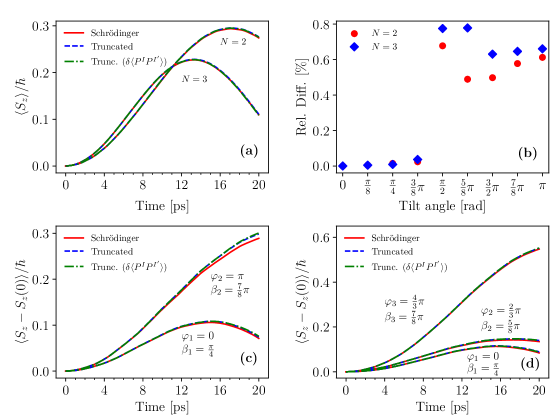
Figure 1: (a): Time evolution of the impurities’ magnetization along the ring’s axis for an initial polarization of $5\hbar/2$ along the $x$ axis. The solid curve correspond to the exact (Schrödinger) solution, while the dashed and dash-dotted lines to those obtained using the truncation scheme including and leaving out the correlations $\delta\langle P^{I}P^{I^{\prime}}\rangle$. (b): Maximum difference between the approximate and the referece solutions, computed relative to the latter, for different tilt angles and without the $\delta\langle P^{I}P^{I^{\prime}}\rangle$. (c-d): Same as (a) but assuming a different initial tilt angle $\beta_{I}$ for each of the $N=2$ (c) or $N=3$ (d) impurities located at $\varphi_{I}$. For clarity, the magnetization is shown relative to its initial value. In all cases, the electron starts in the state $|1\uparrow\rangle$.

Let us first assume that all the impurities’ spins have been maximally polarized along the $x$ axis, that is $\beta=\pi/2$ and $\langle S_{x}^{I}\rangle=5\hbar/2$ and $\langle S_{y,z}^{I}\rangle=0$ for all $I$. In Fig. 1a we pick one of the $N$ impurities in the system and display the time evolution of its magnetization along the ring’s axis. Which impurity we pick is immaterial, since all of them show the same spin dynamics as a consequence of their highly symmetrical spatial distribution on the ring (see Appendix B). The solid line corresponds to the reference (exact) solution obtained in the Schrödinger picture, while the dashed and dash-dotted lines show the dynamics of the same quantity as described by the truncation scheme with and without the direct impurity-impurity correlation $\delta\langle P^{I}P^{I^{\prime}}\rangle$, respectively. We see that in the time range considered, the approximate solutions including and leaving out this latter correlation are in excellent agreement with one another and each with the reference solution. When the spins are aligned at different angles, the approximate solutions differ from the reference in no more than $1\%$ when their separation reaches the global maximum (Fig. 1b). The same close correspondence is observed for a variety of randomly chosen initial states, as well as for the case in which the impurities’ spins are aligned at different tilt angles. A particular example of this case is presented in Fig. 1c for $N=2$ and in Fig. 1d for $N=3$. The addition of the equations for $\langle P^{I}P^{I^{\prime}}\rangle$ to the original set is of no consequence at all, as expected in the highly-diluted limit. We observe that in these situations, and when the average distance between the manganese atoms is large enough, the impurity-impurity exchange terms may be safely approximated by their mean-field contributions.

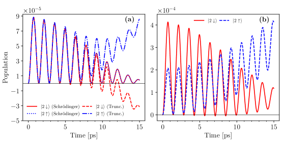
Figure 2: (a): Time evolution of the population of the electronic states $|2\uparrow\rangle$ and $|2\downarrow\rangle$ for the exact solution (solid lines) and the approximate one (dashed lines) not considering the contributions of the $\delta\langle P^{I}P^{I^{\prime}}\rangle$. We assume that, initially, all impurities’ spins are equally and maximally polarized along the $x$ axis ($\beta=\pi/2$). (b): Population of the same electronic states but for the case in which the impurities’ spins are initially oriented at random. In both figures we consider $N=3$ and the same initial electron state as in Fig. 1.

The truncation scheme is, however, not so accurate in approximating the transitions into and out of the available electron states. For the impurities initially in the $S_{x}$ eigenstate of maximum projection ($\beta=\pi/2$) and an electron in the $|1\uparrow\rangle$ state, the populations of the states $|2\uparrow\rangle$ and $|2\downarrow\rangle$ are over- and underestimated throughout the time range considered (Fig. 2a), respectively. The discrepancy is worsened by the fact that the approximated populations eventually take on negative values that, because of their magnitude, cannot be ascribed to numerical error. This behavior is observed as well for smaller integration time steps and different initial states for the electron and the impurities’ spins. In particular, it is observed when the latter are oriented at random; that is, when their state is initially described by the condition $P^{I}_{n_{1}n_{2}}(t=0)=\frac{1}{6}\delta_{n_{1}n_{2}}$ for all $I$ (Fig. 2b). In treating this case we make the additional assumption that correlations $\delta\langle c_{m_{1}\sigma_{1}}^{{\dagger}}c_{m_{2}\sigma_{2}}P^{I}_{n_{1}n_{2}}\rangle$ take time to build upThurn and Axt (2012) and are therefore initially zero (that is, the electron’s and the impurities’ states are not initially entangled.) However, regardless of the initial condition considered, the approximation always respects the hermiticy of all two- and three-point density matrices in the set of truncated equations. Negative values for the populations therefore indicate that the positive semi-definiteness of the electronic density matrix is not conserved during time evolution.

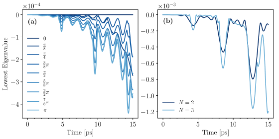
Figure 3: (a): Lowest eigenvalue of the electronic density matrix $\langle c_{m_{1}\sigma_{1}}^{{\dagger}}c_{m_{2}\sigma_{2}}\rangle$ for the $N=3$ case and all impurities’ spins initially on the $xz$ plane and oriented at the same tilt angle with respect to the ring’s axis. (b): Same as (a) but for the randomly oriented ensemble. We assume the electron in the same initial state as in Fig. 2.

This is revealed by the sign of its lowest eigenvalue, which is negative in all but one of the cases presented in Figs. 3a-b. In fact, the electronic density matrix becomes indefinite right at the first integration step not only for the particular case $\beta=\pi/2$, but also for other initial tilt angles (Fig. 3a), as well as for the case in which the impurities’ spins are oriented completely at random (Fig. 3b). Notice that the hermiticity of each truncated density matrix can be guaranteed directly on the right-hand side of its equation of motion, since this property depends at most on the density matrices themselves. In contrast, their positive semi-definiteness requires a condition on their second time derivative, and therefore depends strongly on $Q$. The difference between both properties is most clearly reflected in the negative populations shown in Figs. 2a-b. Hermiticity of the whole density matrix requires the populations to be real (not necessarily positive), but its positive semi-definiteness requires in addition that they reach a local minimum whenever they become zero. From Eq. (7), it is not hard to see that this condition depends on the first time derivative of the quantities $\langle c_{m_{1}\sigma_{1}}^{{\dagger}}c_{m_{2}\sigma_{2}}P^{I}_{n_{1}n_{2}}\rangle$ and therefore directly on the truncated term $Q$. This is also the case for the other density matrices in the truncated set. Adding the direct impurity-impurity exchange term only introduces small corrections to the values of the populations but does not help at all to solve or reduce this problem. The $\langle P^{I}\rangle$ matrices also lose their initial positive semi-definiteness as their elements evolve in time. It is only when the impurities’ spins are maximally polarized along the axis of the ring that this problem does not arise. When this happens the spin part of the initial ket is the eigenstate of maximum projection ($5N/2+1/2$) of the total SAM, which is a conserved quantity. Neither the electron’s nor the impurities’ spins therefore change in time, since there are no other available states for them to flip to while keeping the maximum projection constant. Whether correlations of the electron-mediated impurity-impurity interaction are neglected or not is irrelevant to the dynamics in this case, and this is reflected in the conservation of the positive semi-definiteness of the electronic density matrix. Nevertheless, the relevance of these correlations for the computation of the observables grows as the number of available total spin states increases. This is clearly exemplified in Fig. 2b by the abrupt change in the relative difference between the approximate and the exact magnetization of the impurities when $\beta=\pi/2$.

V Concluding remarks

In this work we studied the quantum dynamics of a quasi-one-dimensional DMS quantum ring. The focus was on testing the methodological difficulties that appear when employing the Heisenberg equations of motion to calculate the dynamics of the electron and impurities’ density matrices. Following a standard scheme for DMS in the bulk, we truncated the infinite hierarchy of equations by neglecting all direct impurity-impurity correlations and reducing the indirect electron-mediated interaction to its mean-field terms. Through this approach we obtained an approximate and numerically tractable set of equations that goes beyond traditional mean-field approximations of the full Hamiltonian.

In order to study the features and limitations of the truncation scheme, we considered a small system of one electron and few magnetic impurities initially in a pure state. We integrated the exact time-dependent Schrödinger equation and used it to compute the impurities’ magnetization and the population of the electronic states. These results set a benchmark that allowed us to assess the accuracy of the truncated set of equations. We found that neglecting the indirect impurity-impurity correlations altogether does not break the fundamental symmetries of the system, but nevertheless leads to a non strictly Hamiltonian time evolution. For different initial states (with and without entanglement between the impurities) and a variety of initial configurations, we found that the energy, the total SAM, the number of particles, and the hermiticity of the density matrices are conserved to numerical precision. The conservation of the number of particles (i.e., the traces of the electronic and the $\langle P^{I}\rangle$ density matrices) is indicative that errors in the populations are, up to numerical precision, exactly compensated at each time step. However, for some populations we observed a small but negative drift that leads them to take on negative values which could not be ascribed to numerical error. The positive semi-definiteness of the density matrices is therefore not conserved throughout the time range studied. In fact, in most cases it breaks right at the first time step. From a theoretical point of view, this problem is rather serious and must be addressed before using the truncated set of equations to study the physics of a DMS QR in depth, particularly when no exact solution is at hand. In practice, however, we saw that the approximation yields a remarkably accurate estimation of an observable like the impurities’ magnetization in the same time range. We conclude that, under certain conditions, the truncation scheme can still be applied to study the dynamics of some physical quantities, particularly those that are not too sensitive to errors in the populations, in time scales longer than those of traditional time-dependent perturbation theory.

Finally, we mention that the problem of guaranteeing the positive semidefiniteness of a truncated or approximated density matrix has been studied in other areas of many-body physics. A case in point is the field of atomic and molecular physics and the theory of reduced density matrices (see Ref. [Mazziotti, 2007]), which provides methods for computing physical properties of systems with many interacting electrons using only low-order density matrices (that is, density matrices involving few electronic creation and annihilitation operators). It is known that such methods can sometimes yield density matrices that are not positive semidefinite and need to be corrected. This is in fact possible, but the procedure for correcting (or “purifying”) one particular density matrix in general requires imposing conditions on other density matrices of lower order as well (see Ref. [Alcoba, 2007] and references therein).

This is also the case for the problem presented here, as any further approximation carried out on any of the density matrices would require guaranteeing also the conservation of the energy and total SAM, without breaking the symmetries of the system, which, as we mentioned, are respected by the original truncation scheme. Such constraints couple all density matrices. Some particular instances of this problem may be tackled using the techniques of semidefinite programming or the theory of convex optimization, for example to replace each density matrix with its optimal projection in the space of positive semidefinite ones that satisfy the required constraints. However, such a complex optimization problem would have to be solved after each numerical integration step, since positive semidefiniteness is not conserved, and even for a small number of impurities its computational cost may be prohibitively high. Furthermore, such mathematical approaches do not necessarily follow meaningful physical criteria that one may wish to enforce. A solution that tackles the core of the physical problem directly in the truncation scheme itself would therefore be more desirable. This work aims to contribute to the search of such a solution by singling out a serious drawback present in the conventional truncation scheme of the hierarchy of dynamical equations of motion of the density matrices.

Appendix A

The Heisenberg equations for the quantities $\langle P^{I}P^{I^{\prime}}\rangle$ involve only commutators of the form $[P^{I}P^{I^{\prime}},P^{I^{\prime\prime}}]$ which again yield terms proportional to $P^{I}P^{I^{\prime}}$. As a consequence, the time evolution of each $\langle P^{I}P^{I^{\prime}}\rangle$ depends only on four-point density matrices $\langle c^{{\dagger}}_{\lambda_{1}}c_{\lambda_{2}}P^{I}P^{I^{\prime}}\rangle$. If, as in the expression for $Q$, these four-point matrices are expanded according to Eq. (10) and all factors $\delta\langle P^{I}P^{I^{\prime}}\rangle$ are expressed in terms of their correlated and mean-field parts, it follows that dropping the term $\delta\langle c^{{\dagger}}_{\lambda_{1}}c_{\lambda_{2}}P^{I}P^{I^{\prime}}\rangle$ suffices to close the set of equations at the three-point level. It is therefore possible to add the Heisenberg equations for the quantities $\langle P^{I}P^{I^{\prime}}\rangle$ when $I\neq I^{\prime}$ to the original set containing Eqs. (6), (7) and (8) while keeping it closed at the three-point level and without introducing further approximations.

Appendix B

Let us assume that the impurities are located at the vertices of an $N$-sided regular polygon and consider a rotation $R$ in the dihedral group $D_{N}$. The operation $RHR^{{\dagger}}$ leaves the operators $L_{z}^{2}$ and $\mathbf{S}_{I}\cdot\mathbf{s}$ invariant, but shifts the arguments of the delta function operators by an integer multiple of $2\pi/N$. This translation along the ring is a cyclic permutation that relocates the impurities to different vertices on the same polygon, because it maps each parameter $\varphi_{I}$ to some other $\varphi_{I^{\prime}}$ (modulo $2\pi$). The rotated Hamiltonian can also be obtained by permuting the operators $\mathbf{S}_{I}$ instead of shifting the delta potentials. That is, the operation $RHR^{{\dagger}}$ is equivalent to $\hat{O}_{R}H\hat{O}_{R}^{{\dagger}}$, for some $\hat{O}_{R}$ that relabels the $\mathbf{S}_{I}$ without affecting the parameters $\varphi_{I}$. The operator $\hat{O}_{R}$ can be written as a product of pairwise permutations $\hat{O}_{II^{\prime}}\doteq\sum_{n_{1}n_{2}}P^{I}_{n_{1}n_{2}}P^{I^{\prime}}_{n_{2}n_{1}},$ that interchanges two impurities in $H_{sd}$ by swapping the indices $I$ and $I^{\prime}$ ($I\neq I^{\prime}$) of the operators $\mathbf{S}_{I}$ and $\mathbf{S}_{I^{\prime}}$. Notice that $\hat{O}_{II^{\prime}}^{-1}=\hat{O}_{I^{\prime}I}=\hat{O}_{II^{\prime}}^{{\dagger}}=\hat{O}_{II^{\prime}}$ as required.

Let us decompose the rotation $R$ into a product of two rotations, $R=R_{\text{OAM}}R_{\text{SAM}}$, one acting only on the electron’s OAM and the other acting on its spin and the impurities’ SAM, and consider the ket $|\psi\rangle=|m\sigma\rangle|\text{Mn}\rangle\cdots|\text{Mn}\rangle$, where $|m\sigma\rangle$ is an eigenstate of the operators $L_{z}$ and $s_{z}$ with eigenvalues $m$ and $\sigma$ respectively, and $|\text{Mn}\rangle$ an arbitrary single-impurity state that is repeated $N$ times in the product. Notice that $|\psi\rangle$ is an eigenstate of $R_{\text{OAM}}$ and of $O_{R}$ for any rotation $R$, since swapping any pair of $|\text{Mn}\rangle$ factors in $|\psi\rangle$ does not change the latter. Calling $\mathcal{U}(t)$ the time-evolution operator and $S_{z}^{I}$ the $z$-component of $\mathbf{S}_{I}$ in the Schrödinger picture, we write

$$\langle\psi|\mathcal{U}^{{\dagger}}S_{z}^{I}\mathcal{U}|\psi\rangle =\langle\psi|\hat{O}_{R}^{{\dagger}}R\mathcal{U}^{{\dagger}}R^{{\dagger}}\hat{O}_{R}S_{z}^{I}\hat{O}_{R}^{{\dagger}}R\mathcal{U}R^{{\dagger}}\hat{O}_{R}|\psi\rangle=\langle\psi|R_{\text{SAM}}^{{\dagger}}\mathcal{U}^{{\dagger}}S_{z}^{I^{\prime}}\mathcal{U}R_{\text{SAM}}|\psi\rangle$$ (11)

$$=\langle\psi|R_{\text{SAM}}^{{\dagger}}\mathcal{U}^{{\dagger}}S_{z}^{I^{\prime}}\mathcal{U}R_{\text{SAM}}|\psi\rangle=\langle\psi|\mathcal{U}^{{\dagger}}S_{z}^{I^{\prime}}\mathcal{U}|\psi\rangle$$

The second equality on the right-hand side follows from the equalities $\hat{O}_{R}^{{\dagger}}S_{z}^{I}\hat{O}_{R}=S_{z}^{I^{\prime}}$ for some $I^{\prime}\neq I$, and $[S_{z}^{I},R]=0$ for all $R$. The fourth equality follows instead from the invariance of $H$ with respect to spin-only rotations; that is, $[R_{\text{SAM}},H]=0$.

References

- Thurn and Axt (2012) C. Thurn and V. M. Axt, Phys. Rev. B 85, 165203 (2012).
- Aarts et al. (2000) G. Aarts, G. F. Bonini, and C. Wetterich, Phys. Rev. D 63, 025012 (2000).
- Leymann et al. (2014) H. A. M. Leymann, A. Foerster, and J. Wiersig, Phys. Rev. B 89, 085308 (2014).
- Xu and Yan (2007) R.-X. Xu and Y.-J. Yan, Phys. Rev. E 75, 031107 (2007).
- Kubo (1962) R. Kubo, J. Phys. Soc. Jpn. 17, 1100 (1962).
- Axt and Stahl (1994) V. M. Axt and A. Stahl, Zeitschrift für Physik B Condensed Matter 93, 195 (1994).
- Rossi and Kuhn (2002) F. Rossi and T. Kuhn, Rev. Mod. Phys. 74, 895 (2002).
- Khitrova et al. (1999) G. Khitrova, H. M. Gibbs, F. Jahnke, M. Kira, and S. W. Koch, Rev. Mod. Phys. 71, 1591 (1999).
- Lindberg et al. (1994) M. Lindberg, Y. Z. Hu, R. Binder, and S. W. Koch, Phys. Rev. B 50, 18060 (1994).
- Ungar et al. (2017) F. Ungar, M. Cygorek, and V. M. Axt, Phys. Rev. B 95, 245203 (2017).
- Ungar et al. (2018) F. Ungar, M. Cygorek, and V. M. Axt, Phys. Rev. B 97, 045210 (2018).
- Kacman (2001) P. Kacman, Semiconductor Science and Technology 16, R25 (2001).
- Blinowski and Kacman (2003) J. Blinowski and P. Kacman, Phys. Rev. B 67, 121204(R) (2003).
- Morandi et al. (2009) O. Morandi, P.-A. Hervieux, and G. Manfredi, New Journal of Physics 11, 073010 (2009).
- Chang et al. (2004) K. Chang, S. S. Li, J. B. Xia, and F. M. Peeters, Phys. Rev. B 69, 235203 (2004).
- Wu et al. (2010) M. Wu, J. Jiang, and M. Weng, Physics Reports 493, 61 (2010).
- Ma (2013) X. Ma, Journal of Materials Science 48, 2111 (2013).
- Krainov et al. (2017) I. V. Krainov, M. Vladimirova, D. Scalbert, E. Lähderanta, A. P. Dmitriev, and N. S. Averkiev, Phys. Rev. B 96, 165304 (2017).
- Ungar et al. (2019) F. Ungar, M. Cygorek, and V. M. Axt, Phys. Rev. B 99, 195309 (2019).
- Viefers et al. (2004) S. Viefers, P. Koskinen, P. Singha Deo, and M. Manninen, Physica E: Low-dimensional Systems and Nanostructures 21, 1 (2004).
- Dietl (2010) T. Dietl, Nature Materials 9, 965 (2010).
- Dietl and Ohno (2014) T. Dietl and H. Ohno, Rev. Mod. Phys. 86, 187 (2014).
- Frustaglia and Richter (2004) D. Frustaglia and K. Richter, Phys. Rev. B 69, 235310 (2004).
- Yakovlev and Merkulov (2010) D. R. Yakovlev and I. A. Merkulov, “Spin and energy transfer between carriers, magnetic ions, and lattice,” in Introduction to the Physics of Diluted Magnetic Semiconductors, edited by J. A. Gaj and J. Kossut (Springer Berlin Heidelberg, Berlin, Heidelberg, 2010) pp. 263–303.
- Kondo (1964) J. Kondo, Progress of Theoretical Physics 32, 37 (1964).
- Lia and Tamborenea (2021) J. M. Lia and P. I. Tamborenea, Physica E: Low-dimensional Systems and Nanostructures 126, 114419 (2021).
- Lia et al. (2022) J. M. Lia, P. I. Tamborenea, M. Cygorek, and V. M. Axt, Phys. Rev. B 105, 115426 (2022).
- Qu and Hawrylak (2005) F. Qu and P. Hawrylak, Phys. Rev. Lett. 95, 217206 (2005).
- Meijer et al. (2002) F. E. Meijer, A. F. Morpurgo, and T. M. Klapwijk, Phys. Rev. B 66, 033107 (2002).
- Lorke et al. (2000) A. Lorke, R. J. Luyken, A. O. Govorov, J. P. Kotthaus, J. M. Garcia, and P. M. Petroff, Phys. Rev. Lett. 84, 2223 (2000).
- Lin et al. (2009) T.-C. Lin, C.-H. Lin, H.-S. Ling, Y.-J. Fu, W.-H. Chang, S.-D. Lin, and C.-P. Lee, Phys. Rev. B 80, 081304(R) (2009).
- Sheng and Chang (2007) J. S. Sheng and K. Chang, Journal of Physics: Condensed Matter 20, 025222 (2007).
- Chakraborty and Pietiläinen (1994) T. Chakraborty and P. Pietiläinen, Phys. Rev. B 50, 8460 (1994).
- Shakouri et al. (2012) K. Shakouri, B. Szafran, M. Esmaeilzadeh, and F. M. Peeters, Phys. Rev. B 85, 165314 (2012).
- Furdyna (1988) J. K. Furdyna, Journal of Applied Physics 64, R29 (1988).
- Quinteiro and Tamborenea (2009) G. F. Quinteiro and P. I. Tamborenea, Phys. Rev. B 79, 155450 (2009).
- Quinteiro et al. (2011) G. F. Quinteiro, P. I. Tamborenea, and J. Berakdar, Opt. Express 19, 26733 (2011).
- Quinteiro Rosen et al. (2022) G. F. Quinteiro Rosen, P. I. Tamborenea, and T. Kuhn, Rev. Mod. Phys. 94, 035003 (2022).
- Mike et al. (2018) P. Mike, L. Z. Szabó, and P. Földi, Journal of Russian Laser Research 39, 465 (2018).
- Kneip et al. (2006) M. K. Kneip, D. R. Yakovlev, M. Bayer, A. A. Maksimov, I. I. Tartakovskii, D. Keller, W. Ossau, L. W. Molenkamp, and A. Waag, Phys. Rev. B 73, 035306 (2006).
- Dietl et al. (1995) T. Dietl, P. Peyla, W. Grieshaber, and Y. Merle d’Aubigné, Phys. Rev. Lett. 74, 474 (1995).
- König et al. (2000) B. König, I. A. Merkulov, D. R. Yakovlev, W. Ossau, S. M. Ryabchenko, M. Kutrowski, T. Wojtowicz, G. Karczewski, and J. Kossut, Phys. Rev. B 61, 16870 (2000).
- Mazziotti (2007) D. A. Mazziotti, ed., Reduced‐Density‐Matrix Mechanics: With Application to Many‐Electron Atoms and Molecules (John Wiley & Sons, Ltd, 2007).
- Alcoba (2007) D. R. Alcoba, “Purification of correlated reduced density matrices: Review and applications,” in Reduced‐Density‐Matrix Mechanics: With Application to Many‐Electron Atoms and Molecules (John Wiley & Sons, Ltd, 2007) Chap. 9, pp. 205–259.