On Quantile Treatment Effects, Rank Similarity,
and Variation of Instrumental Variables

Abstract

This paper investigates how certain relationship between observed and counterfactual distributions serves as an identifying condition for treatment effects when the treatment is endogenous, and shows that this condition holds in a range of nonparametric models for treatment effects. To this end, we first provide a novel characterization of the prevalent assumption restricting treatment heterogeneity in the literature, namely rank similarity. Our characterization demonstrates the stringency of this assumption and allows us to relax it in an economically meaningful way, resulting in our identifying condition. It also justifies the quest of richer exogenous variations in the data (e.g., multi-valued or multiple instrumental variables) in exchange for weaker identifying conditions. The primary goal of this investigation is to provide empirical researchers with tools that are robust and easy to implement but still yield tight policy evaluations.

JEL Numbers: C14, C31, C36

Keywords: quantile treatment effects, rank similarity, average treatment effects, endogeneity, multi-valued instrumental variables, partial identification.

1 Introduction

This paper investigates how certain relationship between observed and counterfactual distributions serves as an identifying condition for distributional treatment effects under endogeneity, and shows that this condition holds in a range of nonparametric models for treatment effects. To this end, we first provide a novel characterization of the prevalent assumption restricting treatment heterogeneity in the literature, namely rank similarity. Our characterization demonstrates the stringency of this assumption and allows us to relax it in a economically meaningful way, resulting in our identifying condition. It also justifies the quest of richer exogenous variations in the data (e.g., multi-valued or multiple instrumental variables) in exchange for the weaker identifying condition.

The primary goal of this investigation is to provide empirical researchers with (i) a framework where validity of identifying conditions prescribes the parameters of interest, (ii) tools for identifying and estimating treatment effects that allow for treatment heterogeneity, but that still yield tight policy evaluation and are simple to implement, and (iii) guidance on data collection that leads to drawing informative causal conclusions.

Our analysis centers on the relationship between observed and counterfactual distributions, specifically on the preservation of  first-order stochastic dominance (FOSD) of one distribution over the other to their corresponding counterfactual distributions: for arbitrary compliance types $t,t^{\prime}\in\mathcal{T}$ induced by induced by individuals’ potential treatment responses to instrumental variables (IVs), if

$$Y_{1}|t \prec_{FOSD}Y_{1}|t^{\prime}$$ (1.1)

then

$$Y_{0}|t \prec_{FOSD}Y_{0}|t^{\prime},$$ (1.2)

where $Y_{d}$ denotes the counterfactual outcome given treatment $D=d$. This condition produces a partial ordering of the $Y_{0}$’s distributions based on the partial ordering of the $Y_{1}$’s distributions. As we demonstrate later, this condition can be interpreted as $Y_{0}$ being “noisier” than $Y_{1}$ after controlling for all the confounding variables.

We show that the proposed FOSD-preservation condition enables the identification of certain counterfactual distributions, which are essential components for identifying the treatment effects of our interest. Only for the sake of illustration, consider Imbens and Angrist (1994)’s framework where binary instrument $Z\in\{0,1\}$ influences treatment participation monotonically. Let compliance types $C$, $AT$, and $NT$ stand for compliers, always-takers, and never-takers, respectively. Let $Y$ be the observed outcome given by $Y\equiv DY_{1}+(1-D)Y_{0}$. Suppose the observed distribution satisfies $Y_{1}|AT\prec_{FOSD}Y_{1}|C$. Then the FOSD-preservation condition implies that $Y_{0}|AT\prec_{FOSD}Y_{0}|C$. The latter provides an informative upper bound for $P[Y_{0}\leq y|D=1]$ (and a symmetric analysis provides a lower bound), which is a necessary component in calculating, for example, the quantile treatment effect on the treated (QTT).Although $Y_{1}|AT\prec_{FOSD}Y_{1}|C$ may seem restrictive, this is not generally the case when $Z$ departs from a scalar binary variable. In this sense, our approach underscores the significance of searching for richer exogenous variations of IVs, such as multi-valued or multiple instrumental variables, as a means of trading for less restrictive identifying conditions and achieving tighter bounds. Still, the benefit of our approach can be manifested without requiring continuous or large support of IVs. We also show that the proposed FOSD-preservation condition (i.e., (1.1) implies (1.2)) yields testable restrictions.

Nonparametric identification of treatment effects using IVs with limited support has long been a challenging goal even when the focus is on mean treatment effects, such as the average treatment effect (ATE) and the ATE on the treated (ATT). In an influential line of literature, Manski (1990), Manski (1997), and Manski and Pepper (2000), among many others, construct sharp bounds on the ATE under a set of assumptions on the directions of treatment effects and treatment selection while allowing instruments to be invalid in a specific sense. Even with valid instruments, however, bounds on the ATE are typically wide and uninformative to yield precise policy prediction. The local ATE (LATE) (Imbens and Angrist (1994)) and local QTE (Abadie et al. (2002)) have been a popular alternative when researchers are equipped with discrete IVs and impose a monotonicity assumption on the selection to treatment. However, the local group for which the treatment effect is identified may not be the group of policy interest. Therefore, the extrapolation of the local parameters becomes an important issue for policy analysis (e.g., treatment allocation), in which case the identification challenge still remains (see e.g., Mogstad et al. (2018), Han and Yang (2023)).

Another prevalent approach in the literature is to restrict the degree of treatment heterogeneity via rank similarity (or rank invariance). This assumption has been shown to have substantial identifying power for distributional treatment effects and the ATE and used in various nonparametric contexts implicitly or explicitly (Heckman et al. (1997), Chesher (2003, 2005), Chernozhukov and Hansen (2005), Vytlacil and Yildiz (2007), Jun et al. (2011), Shaikh and Vytlacil (2011), D’Haultfœuille and Février (2015), Torgovitsky (2015), Vuong and Xu (2017), Han (2021) to name a few). However, the plausibility of this assumption can be questionable in many applications (e.g., Maasoumi and Wang (2019)) and testing methods are proposed as one reaction to the skepticism (Frandsen and Lefgren (2018), Dong and Shen (2018), Kim and Park (2022)).

In this paper, we clarify the stringency of the rank similarity assumption by characterizing its restrictions on the relationship between observed and counterfactual distributions. In particular, we show that the strong preservation of FOSD (i.e., (1.1) holds if and only if (1.2) holds) is equivalent to rank linearity, a slight relaxation of rank similarity that allows for a linear transformation of an individual’s rank to the counterfactual rank. By doing so, we establish the connection between the rank similarity assumption introduced by Chernozhukov and Hansen (2005)’s structural IV model and its corresponding conditions within Rubin (1974)’s counterfactual outcomes framework. Furthermore, we provide economic justifications for the weak preservation of FOSD by proposing a variety of non-separable structural IV models that imply the FOSD preservation condition, but that do not satisfy rank similarity.

Based on our identification strategy, we develop a statistical linear programming (LP) approach to estimate optimal bounds on the treatment parameters. These bounds are defined as optimal values of LP (with a discrete outcome) or semi-infinite LP (SILP) (with a continuous outcome). To address the infeasibility of the SILP problem, we transform the optimization problem by (i) randomizing the constraints or (ii) invoking duality and approximates the Lagrangian measure using sieves.

The next section formally introduces the main identifying conditions (i.e., the preservation of stochastic ordering) and establishes bounds on treatment effects. Section 3 introduces structural models as sufficient conditions for the identifying conditions presented in the previous section. Section 4 discusses the computation of the bounds using linear programming and, finally, Section 5 presents numerical studies. In the Appendix, Section A shows that point identification can be achieved with sufficient (but not infinite) variation of IVs. In the main text we focus on the QTE. An extension to bounding the ATE is discussed in Section B. Section C contains more examples of structural models as sufficient conditions and Section D holds further discussions on linear programming. All proofs are collected in Section E.

2 Key Conditions and Bounds on Treatment Effects

Let $D\in\{0,1\}$ be the observed treatment indicator, which represents the endogenous decision of an individual responding to IVs $Z$. We assume $Z$ is either a vector of binary IVs or a multi-valued IV, which takes $L$ distinct values: $Z\in\mathcal{Z}\equiv\{z_{1},...,z_{L}\}$. Multi-valued or multiple IVs are common in many observational studies (e.g., natural experiments typically provide more than one instrument) and experimental studies (e.g., randomized control trials where multiple treatment arms are implemented either simultaneously or sequentially). Let $Y_{1}$ be the counterfactual outcome of being treated and $Y_{0}$ be that of not being treated. They can be either continuously or discretely distributed. The observed outcome $Y\in\mathcal{Y}\subseteq\mathbb{R}$ satisfies $Y=DY_{1}+(1-D)Y_{0}$. Finally, $X\in\mathcal{X}\subseteq\mathbb{R}^{k}$ denotes other covariates that may be endogenous.

Define QTE and ATE for treated and untreated populations. For $d\in\{0,1\}$ and $x\in\mathcal{X}$, define

$$QTE_{\tau}(d,x) =Q_{Y_{1}|D,X}(\tau|d,x)-Q_{Y_{0}|D,X}(\tau|d,x)$$

for $\tau\in(0,1)$ and

$$ATE(d,x) =E[Y_{1}-Y_{0}|D=d,X=x].$$

These parameters are what researchers and policymakers are potentially interested. The unconditional QTE and ATE can be recovered when these parameters are identified for all $d\in\{0,1\}$ and $x\in\mathcal{X}$. Throughout the paper, we maintain that the IVs are valid and satisfy the following exclusion restriction.

Assumption Z.

For $d\in\{0,1\}$, $Z\perp Y_{d}|X$.

2.1 Introducing Key Conditions

Now we introduce the key condition that establishes the mapping between observed and counterfactual distributions.

Condition S₁.

For arbitrary non-negative weight vectors $(w_{1},...,w_{L})$ and $(\tilde{w}_{1},...,\tilde{w}_{L})$ that satisfy $\sum_{\ell=1}^{L}w_{\ell}=\sum_{\ell=1}^{L}\tilde{w}_{\ell}=1$, if

$$\sum_{\ell=1}^{L}w_{\ell}P[Y_{1}\leq\cdot|D=1,Z=z_{\ell},X=x] \leq\sum_{\ell=1}^{L}\tilde{w}_{\ell}P[Y_{1}\leq\cdot|D=1,Z=z_{\ell},X=x],$$ (2.1)

then

$$\sum_{\ell=1}^{L}w_{\ell}P[Y_{0}\leq\cdot|D=1,Z=z_{\ell},X=x] \leq\sum_{\ell=1}^{L}\tilde{w}_{\ell}P[Y_{0}\leq\cdot|D=1,Z=z_{\ell},X=x].$$ (2.2)

Importantly, note that in (2.1) the probability $P[Y_{1}\leq\cdot|D=1,Z=z_{\ell},X=x]$ can be obtained from the data as $Y_{1}=Y$ given $D=1$. The mapping between observed and counterfactual distributions has been considered in Vuong and Xu (2017), whose insights we share. Suppose that $Z\perp(Y_{d},D_{z})|X$ additionally holds, where $D_{z}$ is the counterfactual treatment given $Z=z$. Under this assumption, each probability term in Condition S₁ satisfies $P[Y_{d}\leq\cdot|D=1,Z=z_{\ell},X=x]=P[Y_{d}\leq\cdot|D_{z_{\ell}}=1,X=x]$. Note that $\sum_{\ell=1}^{L}w_{\ell}P[Y_{1}\leq\cdot|D_{z_{\ell}}=1,X=x]$ is a mixture of $Y_{d}$’s distributions weighted across different compliance types defined by $\{D_{z_{\ell}}=1\}$, and thus can be viewed as a distribution for a hypothetical population with the specific composition of compliance types. Therefore, Condition S₁ posits that the FOSD ordering between the $Y_{1}$’s distributions of two compliance compositions is preserved between their counterfactual distributions of $Y_{0}$. For example, when $L=2$ and defiers are excluded from possible compliance types (e.g., by Imbens and Angrist (1994)’s monotonicity assumption), then Condition S₁ simply describes the stochastic ordering between always-takers and compliers. When $L\geq 3$, however, there are more compliance types, which composition becomes more complex as illustrated in Section 2.3. Note that Condition S₁ is not an “if and only if” statement. It would be stringent to impose the preservation of ordering to hold in both directions. In fact, such a condition is closely related to the rank similarity condition (Chernozhukov and Hansen (2005)); see Section 3 for full details.

2.2 Bounds on Treatment Effects

Now, we show that Condition S₁ is useful in constructing bounds on $F_{Y_{0}|D,X}(\cdot|1,x)$ and subsequently on $QTE_{\tau}(1,x)$. Let $p(z_{\ell},x)\equiv P[D=1|Z=z_{\ell},X=x]$ and

$$\Gamma(x) \equiv\left\{(\gamma_{1},...,\gamma_{L})\in\mathbb{R}^{L}:\sum_{\ell=1}^{L}\gamma_{\ell}=0\text{ and }\sum_{\ell=1}^{L}\gamma_{\ell}p(z_{\ell},x)=1\right\}.$$

Theorem 2.1.

Suppose that Assumption Z and Condition S₁ hold. Fix $x\in\mathcal{X}$. For $\gamma\equiv(\gamma_{1},...,\gamma_{L})$ and $\tilde{\gamma}\equiv(\tilde{\gamma}_{1},...,\tilde{\gamma}_{L})$ in $\Gamma(x)$, suppose

$$P[Y\leq\cdot|D=1,X=x]\leq\sum_{\ell=1}^{L}\gamma_{\ell}P[Y\leq\cdot,D=1|Z=z_{\ell},X=x],$$ (2.3)

$$\sum_{\ell=1}^{L}\tilde{\gamma}_{\ell}P[Y\leq\cdot,D=1|Z=z_{\ell},X=x]\leq P[Y\leq\cdot|D=1,X=x].$$ (2.4)

Then $F_{Y_{0}|D,X}(\cdot|1,x)$ is bounded by

$$-\sum_{\ell=1}^{L}\tilde{\gamma}_{\ell}P[Y\leq\cdot,D=0|Z=z_{\ell},X=x]$$ (2.5)

$$\leq P[Y_{0}\leq\cdot|D=1,X=x]$$

$$\leq-\sum_{\ell=1}^{L}\gamma_{\ell}P[Y\leq\cdot,D=0|Z=z_{\ell},X=x]$$ (2.6)

Remark 2.1 (Constraints on $\gamma$).

In Theorem 2.1, $\Gamma(x)$ imposes two restrictions on $\gamma$: (i) $\sum_{\ell=1}^{L}\gamma_{\ell}=0$ and (ii) $\sum_{\ell=1}^{L}\gamma_{\ell}p(z_{\ell},x)=1$. First, note that the existence of such a sequence requires the relevance of the IV: $p(z_{\ell},x)\neq p(z_{\ell^{\prime}},x)$ for some $z_{\ell},z_{\ell^{\prime}}$. Second, note that (ii) is a condition implied by either (2.3) or (2.4) with $y\rightarrow\infty$. Restriction (ii) implicitly introduces a scale normalization. That is, for any $\gamma$ satisfying $\sum_{\ell=1}^{L}\gamma_{\ell}p(z_{\ell},x)\neq 0$, we can always rescale it as $\gamma^{*}=\frac{\gamma}{\sum_{\ell=1}^{L}\gamma_{\ell}p(z_{\ell},x)}$ so that $\sum_{\ell=1}^{L}\gamma_{\ell}p(z_{\ell},x)=1$. It can be shown that this normalization does not affect the bounds obtained in (2.5) and (2.6).

The proof of Theorem 2.1 and most of other proofs are contained in the appendix. Note that there can be multiple $\gamma$ and $\tilde{\gamma}$ in $\Gamma(x)$ that satisfy (2.3) and (2.4), respectively. Therefore, we can further tighten the bounds as follows.

Corollary 2.1.

Suppose that Assumption Z and Condition S₁ hold. Fix $x\in\mathcal{X}$. Then, $F_{Y_{0}|D,X}(\cdot|1,x)$ is upper and lower bounded by

$$F_{Y_{0}|D,X}^{UB}(y|1,x) \equiv\min_{\gamma\in\Gamma(x):\text{\eqref{eq:counter_k} holds}}-\sum_{\ell=1}^{L}\gamma_{\ell}P[Y\leq y,D=0|Z=z_{\ell}],$$

$$F_{Y_{0}|D,X}^{LB}(y|1,x) \equiv\max_{\tilde{\gamma}\in\Gamma(x):\text{\eqref{eq:counter_k2} holds}}-\sum_{\ell=1}^{L}\tilde{\gamma}_{\ell}P[Y\leq y,D=0|Z=z_{\ell}].$$

Theorem 2.1 and Corollary 2.1 highlight the identifying power of multi-valued IVs. The key step in Theorem 2.1 to calculate the bounds is to find $\gamma$ (resp. $\tilde{\gamma}$) in $\Gamma(x)$ that satisfies (2.3) (resp. (2.4)), which serves as a rank condition. Note that this condition is verifiable with the data. Corollary 2.1 additionally implies that the bounds can be further tightened if one increases the degree of freedom in the feasible set $\Gamma(x)$ by increasing $L$, in which case (2.3)–(2.4) are more likely to hold. See below and Section 5 for related discussions.

Finally, note that

$$QTE_{\tau}(1,x)=Q_{Y|D,X}(\tau|1,x)-Q_{Y_{0}|D,X}(\tau|1,x)$$

and the bounds on the second quantity on the right-hand side can be calculated using the worst case bounds for the conditional quantile (Manski (1994), Blundell et al. (2007)):

$$Q_{Y_{0}|D,X}^{LB}(\tau|1,x) \leq Q_{Y_{0}|D,X}(\tau|1,x)\leq Q_{Y_{0}|D,X}^{UB}(\tau|1,x),$$

where $Q_{Y_{0}|D,X}^{LB}(\tau|1,x)$ and $Q_{Y_{0}|D,X}^{UB}(\tau|1,x)$ are the $\tau$-th quantiles of $F_{Y_{0}|D,X}^{LB}(\cdot|1,x)$ and $F_{Y_{0}|D,X}^{UB}(\cdot|1,x)$, respectively. Although the bounds on $ATE(1,x)=E[Y|D=1,X=x]-E[Y_{0}|D=1,X=x]$ can be calculated based on $E[Y_{0}|D=1,X=x]=\int_{0}^{1}Q_{Y_{0}|D,X}(\tau|1,x)d\tau$, we present later how the bounds on the $ATE(d,x)$ can be calculated under a weaker condition than Condition S₁.

If we assume the converse of Condition S₁, we can calculate bounds on the $QTE(0,x)$.

Condition S₀.

For arbitrary non-negative weight vectors $(w_{1},...,w_{L})$ and $(\tilde{w}_{1},...,\tilde{w}_{L})$ that satisfy $\sum_{\ell=1}^{L}w_{\ell}=\sum_{\ell=1}^{L}\tilde{w}_{\ell}=1$, if

$$\sum_{\ell=1}^{L}w_{\ell}P[Y_{0}\leq\cdot|D=0,Z=z_{\ell},X=x] \leq\sum_{\ell=1}^{L}\tilde{w}_{\ell}P[Y_{0}\leq\cdot|D=0,Z=z_{\ell},X=x],$$ (2.7)

then

$$\sum_{\ell=1}^{L}w_{\ell}P[Y_{1}\leq\cdot|D=0,Z=z_{\ell},X=x] \leq\sum_{\ell=1}^{L}\tilde{w}_{\ell}P[Y_{1}\leq\cdot|D=0,Z=z_{\ell},X=x].$$ (2.8)

Similar to Condition S₁, Condition S₀ ensures that if the two distributions of $Y_{0}$ exhibit an FOSD ordering across different compliance compositions, this ordering is preserved in their corresponding counterfactual $Y_{1}$ distributions. In practice, depending on the specific context, Condition S₁, Condition S₀, or both may hold; Section 3 provides some related intuitions. Not surprisingly, we can use Condition S₀ to construct bounds on $F_{Y_{1}|D,X}(\cdot|0,x)$ and subsequently on $QTE_{\tau}(0,x)$.

Theorem 2.2.

Suppose that Assumption Z and Condition S₀ hold. Fix $x\in\mathcal{X}$. For $\gamma\equiv(\gamma_{1},...,\gamma_{L})$ and $\tilde{\gamma}\equiv(\tilde{\gamma}_{1},...,\tilde{\gamma}_{L})$ in $\Gamma(x)$, suppose

$$P[Y\leq\cdot|D=0,X=x]\leq\sum_{\ell=1}^{L}\gamma_{\ell}P[Y\leq\cdot,D=0|Z=z_{\ell},X=x],$$ (2.9)

$$\sum_{\ell=1}^{L}\tilde{\gamma}_{\ell}P[Y\leq\cdot,D=0|Z=z_{\ell},X=x]\leq P[Y\leq\cdot|D=0,X=x].$$ (2.10)

Then $F_{Y_{1}|D,X}(\cdot|0,x)$ is bounded by

$$-\sum_{\ell=1}^{L}\tilde{\gamma}_{\ell}P[Y\leq\cdot,D=1|Z=z_{\ell},X=x]$$ (2.11)

$$\leq P[Y_{1}\leq\cdot|D=0,X=x]$$

$$\leq-\sum_{\ell=1}^{L}\gamma_{\ell}P[Y\leq\cdot,D=1|Z=z_{\ell},X=x].$$ (2.12)

The proof of this theorem is analogous to that of Theorem 2.1. The bounds on $QTE_{\tau}(0,x)$ can be derived symmetrically as in the case of $QTE_{\tau}(1,x)$ and thus are omitted. Notably, which treatment parameter we can obtain bounds for is determined by which identifying condition we impose (i.e., Condition S₁ or S₀). In Section 3, we investigate this aspect within economic structural models. Finally, in the Appendix, we introduce weaker conditions to bound average treatment effects.

2.3 Understanding Key Conditions

We further explore Conditions S₁ and S₀ to give additional interpretation and discuss testability. Suppress $X=x$ to simplify our discussions. Under $Z\perp(Y_{d},D_{z})$, the inequalities for FOSD in Conditions S₁ and S₀ can be rewritten as

$$\sum_{\ell=1}^{L}w_{\ell}P[Y_{d}\leq y|D_{z_{\ell}}=1] \leq\sum_{\ell=1}^{L}\tilde{w}_{\ell}P[Y_{d}\leq y|D_{z_{\ell}}=1].$$ (2.13)

Recall, Theorem 2.1 relies on the existence of a sequence $\gamma=(\gamma_{1},...,\gamma_{L})$ satisfying $\sum_{\ell=1}^{L}\gamma_{\ell}=0$, $\sum_{\ell=1}^{L}\gamma_{\ell}p(z_{\ell},x)=1$, and the inequality (2.3), that is, $P[Y\leq y|D=1]\leq\sum_{\ell=1}^{L}\gamma_{\ell}P[Y\leq y,D=1|Z=z_{\ell}]$ for all $y$. Note that (2.3) is a special case of (2.13) with $d=1$, which is the “if” part of Condition S₁. Let $p(z)\equiv(D=1|Z=z)$. Only for the purpose of this subsection, assume the generalized version of the LATE monotonicity introduced in Imbens and Angrist (1994):

$$\text{For }\ell\neq\ell^{\prime}, \text{ either }D_{z_{\ell}}\geq D_{z_{\ell^{\prime}}}\text{ a.s. or }D_{z_{\ell}}\leq D_{z_{\ell^{\prime}}}\text{ a.s.}$$ (2.14)

Under (2.14), $\{D_{z_{\ell}}=1\}$ in (2.13) are a mix of individuals who are compliers (C) and always-takers (AT). For $Z\in\mathcal{Z}=\{z_{1},...,z_{L}\}$, let $(z_{\ell-1},z_{\ell})$-compliers be compliers induced by the change of $Z$ from $z_{\ell-1}$ to $z_{\ell}$. When $L=3$ and $(z_{1},z_{2},z_{3})=(0,1,2)$, for example, $\{(0,1)\text{-C}\}=\{i:D_{0,i}=0,D_{1,i}=D_{2,i}=1\}$ is the set of eager compliers (E-C) and $\{(1,2)\text{-C}\}=\{i:D_{0,i}=D_{1,i}=0,D_{2,i}=1\}$ is the set of reluctant compliers (R-C), following the language of Mogstad et al. (2021). Also, $\{\text{AT}\}=\{i:D_{0,i}=D_{1,i}=D_{2,i}=1\}$ is the set of always-takers. Let $p_{\ell}$ for $\ell=\{2,...,L\}$ is the proportion of $(z_{\ell-1},z_{\ell})$-compliers and let $p_{1}\equiv P[\text{AT}]$. We show that (2.13) establishes the FOSD relationship between the mixtures of observed distributions of $Y$ conditional on various always-takers and compliers groups:

Lemma 2.1.

Suppose (2.14) holds and $Z\perp(Y_{d},D_{z})$ and $0<p(z_{\ell})<1$ for all $\ell$. (i) Then, (2.13) is equivalent to

$$\omega_{1}P[Y_{d}\leq y|\text{AT}]+\sum_{\ell=2}^{L}\omega_{\ell}P[Y_{d}\leq y|(z_{\ell-1},z_{\ell})\text{-C}]$$

$$\leq\tilde{\omega}_{1}P[Y_{d}\leq y|\text{AT}]+\sum_{\ell=2}^{L}\tilde{\omega}_{\ell}P[Y_{d}\leq y|(z_{\ell-1},z_{\ell})\text{-C}]$$

for some non-negative $\omega_{\ell}$ and $\tilde{\omega}_{\ell}$ for $\ell=1,...,L$. (ii) Moreover, suppose $L\geq 2$ and $w_{1}+p_{1}\sum_{\ell=2}^{L}\frac{w_{\ell}}{p(z_{\ell})}=\tilde{w}_{1}+p_{1}\sum_{\ell=2}^{L}\frac{\tilde{w}_{\ell}}{p(z_{\ell})}$. Then (2.13) with $w\neq\tilde{w}$ can be expressed as

$$\sum_{\ell=2}^{L}\omega_{\ell}P[Y_{d}\leq y|(z_{\ell-1},z_{\ell})\text{-C}] \leq\sum_{\ell=2}^{L}\tilde{\omega}_{\ell}P[Y_{d}\leq y|(z_{\ell-1},z_{\ell})\text{-C}]$$ (2.15)

for some non-negative $\omega_{\ell}$ and $\tilde{\omega}_{\ell}$ for $\ell=2,...,L$.

To illustrate the intuition of Lemma 2.1(i), consider $L=3$ and $(z_{1},z_{2},z_{3})=(0,1,2)$. Then,

$$\{D_{1}=1\} =\{D_{0}=1,D_{1}=1,D_{2}=1\}\cup\{D_{0}=0,D_{1}=1,D_{2}=1\}=\{\text{AT}\}\cup\{\text{E-C}\},$$

because $\{D_{0}=1,D_{1}=1,D_{2}=0\}=\emptyset$ and $\{D_{0}=0,D_{1}=1,D_{2}=0\}=\emptyset$. Also, $\{D_{2}=1\}=\{\text{AT}\}\cup\{\text{E-C}\}\cup\{\text{R-C}\}$ and $\{D_{0}=1\}=\{\text{AT}\}$.

Lemma 2.1(ii) can be used as the basis to test (2.13) and thus Condition S₁. The intuition is as follows. With a binary IV, the marginal distributions of $Y_{1}$ and $Y_{0}$ are identified for compliers (Abadie et al. (2002)). This result holds for any complier group defined by a pair of instrument values, such as $\{(z_{\ell-1},z_{\ell})\text{-C}\}$ in the lemma. Then, when $L\geq 2$, we can find vectors $w$ and $\tilde{w}$ in $\mathbb{R}_{+}^{L}$ that assign zero weights to the distributions for AT and still make (2.13) a non-trivial inequality where all the associated distributions for compliers are identified for all $d=1,0$.

Remark 2.2 (Conditions w.r.t. Compliance Types).

Motivated from the discussion of this section, we can rewrite Condition S₁ (and all the relevant conditions) solely in terms of compliance types. Let $T\equiv\{D(z_{1}),...,D(z_{L})\}$ be a random vector that indicates a particular compliance type with its realized value in $\{0,1\}^{L}\equiv\tilde{\mathcal{T}}$. For example, when $L=2$ (i.e., binary IV), $T\equiv(D(0),D(1))\in\{(0,0),(1,0),(0,1),(1,1)\}\equiv\tilde{\mathcal{T}}$. Since $D$ and $Z$ are discrete, $T$ is naturally a discrete random vector. Note that this framework do not rely on any selection models, and therefore $T$ captures all possible compliance types given $D$ and $Z$. Then Condition S₁ can be rewritten into the following slightly stringent one:

Fix $x\in\mathcal{X}$. For arbitrary weight functions $w:\tilde{\mathcal{T}}\times\mathcal{X}\rightarrow\mathbb{R}_{+}$ and $\tilde{w}:\tilde{\mathcal{T}}\times\mathcal{X}\rightarrow\mathbb{R}_{+}$ such that $\sum_{t\in\tilde{\mathcal{T}}}w(t,x)=\sum_{t\in\tilde{\mathcal{T}}}\tilde{w}(t,x)=1$, if

$$\sum_{t\in\tilde{\mathcal{T}}}w(t,x)F_{Y_{1}|T,X}(\cdot|t,x)\leq\sum_{t\in\tilde{\mathcal{T}}}\tilde{w}(t,x)F_{Y_{1}|T,X}(\cdot|t,x),$$

then

$$\sum_{t\in\tilde{\mathcal{T}}}w(t,x)F_{Y_{0}|T,X}(\cdot|t,x)\leq\sum_{t\in\tilde{\mathcal{T}}}\tilde{w}(t,x)F_{Y_{0}|T,X}(\cdot|t,x).$$

Then, the weighted sum in each inequality can be interpreted as the distribution of $Y_{d}$ weighted across all compliance types.

3 Structural Models as Sufficient Conditions

We show that Conditions S₁ and S₀ can be justified in a range of nonparametric structural models for the counterfactual outcomes. To this end, it is useful to first present a stronger version of Condition S₁ (labeled as S${}_{1}^{*}$). This version of the condition is motivated by the discussion in Remark 2.2. To state this condition, we introduce a general model for treatment selection:

Assumption D.

Assume that

$$D =h(Z,X,\eta),$$ (3.1)

where $\eta\in\mathcal{T}$ can be an arbitrary vector.

Note that Assumption D permits a more general compliance behavior than what a weakly separable model $D=1\{\eta\leq h(Z,X)\}$ does (or equivalently, (2.14) as shown in Vytlacil (2002)). Although Assumption D is not necessary for our main procedure, it is useful in defining the types of compliance behavior (i.e., treatment selection mechanism) via the unobservable $\eta$. Under this assumption, the following condition implies Condition S₁. Let $F_{Y_{d}|\eta,X}(y|t,x)\equiv P[Y_{d}\leq y|\eta=t,X=x]$.

Condition S${}_{1}^{*}$.

Fix $x\in\mathcal{X}$. For arbitrary weight functions $w:\mathcal{T}\times\mathcal{X}\rightarrow\mathbb{R}_{+}$ and $\tilde{w}:\mathcal{T}\times\mathcal{X}\rightarrow\mathbb{R}_{+}$ such that $\int w(t,x)dt=\int\tilde{w}(t,x)dt=1$, if

$$\int w(t,x)F_{Y_{1}|\eta,X}(\cdot|t,x)dt\leq\int\tilde{w}(t,x)F_{Y_{1}|\eta,X}(\cdot|t,x)dt,$$

then

$$\int w(t,x)F_{Y_{0}|\eta,X}(\cdot|t,x)dt\leq\int\tilde{w}(t,x)F_{Y_{0}|\eta,X}(\cdot|t,x)dt.$$

Because $w(\cdot,x)$ is non-negative and $\int w(t,x)dt=1$, note that $\int w(t,x)F_{Y_{d}|\eta,X}(\cdot|t,x)dt$ is a mixture of conditional CDFs (with $w(\cdot,x)$ being the mixture weight) and thus itself a CDF. In other words, defining a type distribution $W_{x}(t)=\int^{t}w(\eta,x)d\eta$, we can write $\int w(t,x)F_{Y_{d}|\eta,X}(\cdot|t,x)dt=\int F_{Y_{d}|\eta,X}(\cdot|t,x)dW_{x}(t)$. Therefore, Condition S${}_{1}^{*}$ assumes that the FOSD ordering of $Y_{1}$ distributions conditional on $\eta$ conforming to two different type distributions ($W_{x}(\cdot)$ and $\tilde{W}_{x}(\cdot)$) is preserved in the ordering of $Y_{0}$ distributions conditional on the corresponding type distributions.

The following lemma establishes the sufficiency of Condition S${}_{1}^{*}$ for Condition S₁.

Lemma 3.1.

Under Assumption D, Condition S${}_{1}^{*}$ implies Condition S₁.

Symmetrically, Condition S₀ has a corresponding stronger condition, which is omitted.

Now, we relate the conditions with the structural models, which provide additional intuitions for the conditions. We present a leading model here and the rest in the Appendix. For arbitrary r.v.’s $A$ and $\tilde{A}$, let $A\stackrel{{\scriptstyle d}}{{=}}\tilde{A}$ denote $F_{A}=F_{\tilde{A}}$.

Model 1. (i) Assumption D holds and

$$Y =q(D,X,U_{D}),$$ (3.2)

where $q(d,x,\cdot)$ is continuous and monotone increasing and $U_{D}=DU_{1}+(1-D)U_{0}$, (ii) conditional on $(\eta,X,Z)$, $U_{d}\stackrel{{\scriptstyle d}}{{=}}U+\xi_{d}$ where $\xi_{d}\perp(\eta,U)$, (iii) conditional on $(X,Z)$, $\xi_{0}$ is (weakly) more or less noisy than $\xi_{1}$, that is, $\xi_{0}\stackrel{{\scriptstyle d}}{{=}}\xi_{1}+V$ for some $V$ independent of $\xi_{1}$.

Note that $U$ is the source of endogeneity in that it allowed to be dependent on $\eta$. Model 1(ii)–(iii) implies that $U_{0}\stackrel{{\scriptstyle d}}{{=}}U_{1}+V$ conditional on $(\eta,X,Z)$. Importantly, Model 1 nests the model in Chernozhukov and Hansen (2005) as a special case. This can be shown as follows. First, they assume Model 1(i) and, conditional on $(X,Z)$, either rank similarity ($F_{U_{0}|\eta}=F_{U_{1}|\eta}$) or rank invariance ($U_{0}=U_{1}$). Then, by taking $\xi_{d}=0$ for all $d$ in Model 1(ii), we have $U_{0}\stackrel{{\scriptstyle d}}{{=}}U_{1}\stackrel{{\scriptstyle d}}{{=}}U$ conditional on $(\eta,X,Z)$, which proves the claim.

Model 1(iii) assumes that the unobservable under the counterfactual status of being treated are more (or less) dispersed than that under the counterfactually untreated status. Although this may seem stringent, it is substantially weaker than rank similarity (or invariance) and can be plausible in various scenarios. Before providing examples of these scenarios, we first establish the connection between Model 1 and Condition S${}_{1}^{*}$ (and thus Condition S₁ by Lemma 3.1).

Theorem 3.1.

Under Assumptions Z, Model 1 (with $\xi_{0}$ being weakly more noisy than $\xi_{1}$) implies Condition S${}_{1}^{*}$ and thus Condition S₁.

Analogous to Theorem 3.1, one can readily show that Model 1 with $\xi_{0}$ being weakly less noisy than $\xi_{1}$ implies Condition S₀.

Now we provide examples that are consistent with Model 1.

Example 1 (Auction).

Consider online and offline auctions. Let $Y$ be the bid (which subsequently forms revenue) and $D$ be participating in an auction with different format ($D=1$ if online and $=0$ if offline). Let $U_{d}\stackrel{{\scriptstyle d}}{{=}}U+\xi_{d}$ be the valuation of the item where $U$ is the common valuation (correlated with $D$) and $\xi_{d}$ is format specific random shocks satisfying $\xi_{d}\perp(\eta,U)$. We assume that bidders have limited information on certain features of the auction that affect valuation (e.g., they know the distribution of $\xi_{d}$ but not its realization). In this example, what would justify $var(\xi_{0})>var(\xi_{1})$? It may be the case that, in the offline auction, bidders are more emotionally affected by other bidders, which makes their bids more variable.

Example 2 (Insurance).

We are interested in the effect of insurance on health outcomes. Let $Y$ be the health outcome and $D$ be the decision of getting insurance ($D=1$ being insured). Let $U_{d}\stackrel{{\scriptstyle d}}{{=}}U+\xi_{d}$ be underlying health conditions where $U$ captures health conditions known to participant (and thus correlated with $D$) while $\xi_{d}$ is health conditions not fully known a priori and thus random. In this example, $var(\xi_{0})>var(\xi_{1})$ may hold because insurance by definition ensures a certain level of health conditions.

Example 3 (Vaccination).

Similar to Example 2, suppose that $D$ is instead getting vaccination (of an established vaccine). Again, $U_{d}\stackrel{{\scriptstyle d}}{{=}}U+\xi_{d}$ is health conditions where $U$ captures conditions known to participant (and correlated with $D$) and $\xi_{d}$ is vaccination-status-specific health conditions, which are not fully known a priori. Then, similarly as before $var(\xi_{0})>var(\xi_{1})$ may hold because, when not vaccinated, one is exposed to the risk of a serious illness, while vaccination ensures a certain level of immunity.

The scenarios in Examples 1–3 justify Condition S₁ via Theorem 3.1. Then, under Condition S₁, Theorem 2.1 and Corollary 2.1 yield bounds on $QTE_{\tau}(1,x)$, the effects of treatment for those who take the treatment. The final example illustrates the converse case.

Example 4 (Medical Trial).

In contrast to Example 3, suppose the treatment itself is risky. That is, let $D$ be participating in a frontier medical trial ($D=1$ being participation). In this case, $var(\xi_{0})<var(\xi_{1})$ is more plausible because, with a newly developed medicine, there is the high risk of unknown side effects.

The scenario in Example 4 justifies Condition S₀, under which bounds on $QTE_{\tau}(0,x)$, the effects of treatment for those who abstain from it, can be obtained.

Model 1 and these examples show how a certain treatment parameter may be more relevant for policy than others depending on the plausibility of assumptions. Consider the problem of a policymaker. Assume that the policymaker concerns risk-averse individuals, which are typically the majority. For this policymaker, a candidate policy would aim at providing “insurance,” which can be either literally insurance or policies that serve as insurance (e.g., vaccination, subsidies). Therefore, she would be interested in understanding the treatment effects for the target individuals that are risk-averse. Our procedure provides a statistical tool for such a policymaker. That is, under Model 1, our procedure has the ability to bound the treatment effects for individuals with $D=d$ such that $var(\xi_{d})<var(\xi_{1-d})$. This is a unique feature of our setting: the plausibility of assumptions dictates the parameters of interest, which then can be terms as assumption-driven treatment parameters.

A remaining question one might have is as follows. How much Condition S₁ has to be strengthened to be equivalent to rank similarity? To answer this question, recall that Condition S${}_{1}^{*}$ is stronger than Condition S₁ (by Lemma 3.1). We strengthen Condition S${}_{1}^{*}$ further by making it an “if and only if” condition:

Condition S^∗.

Fix $x\in\mathcal{X}$. For arbitrary weight functions $w:\mathcal{T}\times\mathcal{X}\rightarrow\mathbb{R}_{+}$ and $\tilde{w}:\mathcal{T}\times\mathcal{X}\rightarrow\mathbb{R}_{+}$ such that $\int w(t,x)dt=\int\tilde{w}(t,x)=1$, it holds that

$$\int w(t,x)F_{Y_{1}|\eta,X}(\cdot|t,x)dt\leq\int\tilde{w}(t,x)F_{Y_{1}|\eta,X}(\cdot|t,x)dt$$

if and only if

$$\int w(t,x)F_{Y_{0}|\eta,X}(\cdot|t,x)dt\leq\int\tilde{w}(t,x)F_{Y_{0}|\eta,X}(\cdot|t,x)dt.$$

It turns out that we can establish the following result.

Theorem 3.2.

Model 1(i) with $F_{U_{0}|\eta,X,Z}=F_{U_{1}|\eta,X,Z}$ (i.e., rank similarity) implies Condition S^∗.

This theorem highlights the stringency of rank similarity relative to Condition S₁, which is used in our bound analysis. The proof is trivial so omitted. It is worth noting that the converse of Theorem 3.2 is not true. Here is a counter-example for the converse statement.

Definition 3.1 (Rank Linearity).

Assume Model 1(i) and

$$F_{Y_{0}|\eta,X,Z}(\cdot|t,x,z) =\lambda(\cdot,x)F_{Y_{1}|\eta,X,Z}(\psi(\cdot,x)|t,x,z)$$ (3.3)

for every $t\in\mathcal{T}$, $x\in\mathcal{X}$ and $z\in\mathcal{Z}$, where $\psi(\cdot,x):\mathcal{Y}\rightarrow\mathcal{Y}$, a one-to-one and onto mapping, is strictly increasing, and $\lambda(\cdot,x):\mathcal{Y}\rightarrow\mathbb{R}_{+}$ is consistent with $F_{Y_{d}|\eta,X,Z}$ being a proper CDF.

This rank linearity implies Condition S^∗, which is trivial to show. However, rank linearity is weaker than rank similarity as the latter is a special case of the former. To see this, conditional on $Z=z$ (and suppressing $X)$, (3.3) with Model 1(i) yields $F_{U_{0}|\eta}(q^{-1}(0,y)|t)=\lambda(y)F_{U_{1}|\eta}(q^{-1}(1,\psi(y))|t)$. Then, by choosing $\lambda(y)=1$ and $\psi(y)=\phi(y)\equiv q(1,q^{-1}(0,y))$ (i.e., the counterfactual mapping (Vuong and Xu (2017))), we have $F_{U_{0}|\eta}(\cdot|t)=F_{U_{1}|\eta}(\cdot|t)$. In general, while the ranks between $Y_{0}$ and $Y_{1}$ should have the same distribution under rank similarity, their distributions can be different under rank linearity because of the multiplying term $\lambda(\cdot)$ in $F_{U_{0}|\eta}(u|t)=\lambda(q(0,u))F_{U_{1}|\eta}(u|t)$. However, note that the the difference cannot be entirely arbitrary as $\lambda(\cdot)$ does not depend on $t$, and thus rank linearity still poses substantive restrictions.

Interestingly, rank linearity is equivalent to Condition S^∗. The following theorem is one of the main contributions of this paper. Suppress $(Z,X)$ for simplicity.

Theorem 3.3.

Suppose for any CDF $F_{1}(\cdot)$ supported on $\mathbb{R}$, there always exists a function $c:\mathcal{T}\rightarrow\mathbb{R}$ such that

$$F_{d}(\cdot)=\int c(t)F_{Y_{d}|\eta}(\cdot|t)dt.$$ (3.4)

Then Condition S^∗ holds if and only if there exits some $\psi(\cdot)$ that is strictly increasing and $\lambda(\cdot)>0$ such that

$$F_{Y_{0}|\eta}(\cdot|t)=\lambda(\cdot)F_{Y_{1}|\eta}(\psi(\cdot)|t)\qquad\text{for }t\in\mathcal{T}.$$ (3.5)

We prove this equivalence in the Appendix. The proof with continuous $Y_{d}$ is more involved than that with discrete $Y_{d}$; we recommend that the interested reader reads the latter first. The condition (3.4) is only introduced in this theorem to establish the relationship between rank linearity (and hence rank similarity) and the range of identifying conditions of this paper, and it is not necessary for our bound analysis. This condition would be violated when there is no endogeneity (i.e., $Y_{d}\perp\eta$), which is not our focus.

Condition S^∗ is crucial in bounding $QTE_{\tau}(x)=Q_{Y_{1}|X}(\tau|x)-Q_{Y_{0}|X}(\tau|x)$ unconditional with respect to $D=d$. The “only if” part (i.e., Condition S₁) will bound $Q_{Y_{0}|D=1}(\tau)$ and thus $Q_{Y_{0}}(\tau)$ by Theorem 2.1, while the “if” part (i.e., Condition S₀) will bound $Q_{Y_{1}|D=0}(\tau)$ and thus $Q_{Y_{1}}(\tau)$ by the symmetric version of Theorem 2.1. The fact that Condition S^∗ is weaker than rank similarity illustrates the importance of rank similarity in the identification of the QTE and ATE.

Remark 3.1 (Testability of the Conditions).

It is immediate from Lemma 2.1(ii) that Condition S^∗ can be tested from the data when $L\geq 2$ and under the LATE monotonicity assumption. Given the established connection between Condition S^∗ and rank similarity (Theorem 3.2), when Condition S^∗ is refuted from the data, rank similarity can be refuted. This result relates to the testability of rank similarity under LATE monotonicity (Dong and Shen (2018), Kim and Park (2022)).

Remark 3.2 (Conditions w.r.t. Compliance Types, continued).

Continuing the discussion in Remark 2.2, $F_{U_{1}|T,Z}=F_{U_{0}|T,Z}$ (where $T\equiv(D(0),D(1))$ and $X$ is suppressed) can be viewed as an alternative rank similarity assumption. Because $\sigma(T)\subset\sigma(\eta)$ where $\sigma(A)$ is a $\sigma$-field generated by a random vector $A$, $F_{U_{1}|\eta,Z}=F_{U_{0}|\eta,Z}$ implies $F_{U_{1}|T,Z}=F_{U_{0}|T,Z}$. Then Chernozhukov and Hansen (2005)’s main testable implication ((2.6) in Theorem 1 of their paper) can be equally derived under $F_{U_{1}|T,Z}=F_{U_{0}|T,Z}$, which clarifies the role of selection mechanism in their analysis. To see this, let $t\equiv(t_{0},t_{1})$ be the realization of $T\equiv(D(0),D(1))$ and assume Model 1(i). We have

$$P[Y\leq q(D,\tau)|Z=z] =P[q(D,U_{D})\leq q(D,\tau)|Z=z]$$

$$=P[U_{D}\leq\tau|Z=z]$$

$$=\sum_{t\in\tilde{\mathcal{T}}}P[U_{D(z)}\leq\tau|Z=z,T=t]P[T=t|Z=z]$$

but

$$\sum_{t\in\tilde{\mathcal{T}}}P[U_{D(z)}\leq\tau|Z=z,T=t]P[T=t|Z=z] =\sum_{t\in\tilde{\mathcal{T}}}P[U_{t_{z}}\leq\tau|Z=z,T=t]P[T=t|Z=z]$$

$$=\sum_{t\in\tilde{\mathcal{T}}}P[U_{0}\leq\tau|Z=z,T=t]P[T=t|Z=z]$$

$$=P[U_{0}\leq\tau|Z=z]$$

$$=\tau,$$

where $F_{U_{1}|T,Z}=F_{U_{0}|T,Z}$ is used in the second equality and $U_{0}\perp Z$ (imposed in their paper) is used in the last equality.

Note that a slightly weaker version of Condition S^∗ can be stated by replacing $\eta$ with $T$ and the integral with a summation. Then, analogous to Theorem 3.2, one can readily show that $F_{U_{1}|T,Z}=F_{U_{0}|T,Z}$ implies such a condition.

4 Systematic Calculation of Bounds

In Theorem 2.1, $\gamma$ is required to satisfy a set of linear inequality constraints, i.e., (2.3) (respectively, (2.4)), and each feasible $\gamma$ establishes an upper bound (respectively, lower bound) on $F_{Y_{1}|D,X}(\cdot|0,x)$. Therefore, it is intuitive to employ optimization methods to calculate these bounds, as detailed in Corollary 2.1. For simplicity, our subsequent discussion will focus solely on the upper bound, omitting covariates $X$ for brevity.

4.1 Semi-Infinite Programming

To simplify notation, let $\boldsymbol{p}(y,d)\equiv(p(y,d|z_{1}),...,p(y,d|z_{L}))^{\prime}$ where $p(y,d|z_{\ell})\equiv P[Y\leq y,D=d|Z=z_{\ell}]$ and $p(y|d)\equiv P[Y\leq y|D=d]$. Also, let $\boldsymbol{1}\equiv(1,...,1)^{\prime}$ and $\boldsymbol{p}\equiv(p(z_{1}),...,p(z_{L}))^{\prime}$ with $p(z)\equiv P[D=1|Z=z]$ so that

$$\Gamma =\{\gamma:\gamma^{\prime}[\begin{array}[]{cc}\boldsymbol{1}&\boldsymbol{p}\end{array}]=[\begin{array}[]{cc}0&1\end{array}]\}\subset\mathbb{R}^{L}.$$

Consider the following linear semi-infinite programming problem for the upper bound on $P[Y_{0}\leq\bar{y}|D=1]$:

$$UB(\bar{y}) =\min_{\gamma\in\Gamma_{p}}-\boldsymbol{p}(\bar{y},0)^{\prime}\gamma$$ (4.1)

$$s.t. \quad\boldsymbol{p}(y,1)^{\prime}\gamma\geq p(y|1),\quad\forall y\in\mathcal{Y}$$ (4.2)

Note that the existence of $\gamma$ satisfying condition (2.3) guarantees that the feasible set is non-empty. Also note that this condition is allowed to satisfy only almost everywhere (a.e.), which we suppress for simplicity. This program is infeasible to solve in practice as there are infinitely many constraints. We propose two approaches to approximate it with a linear program (LP).

4.2 Linear Program with Randomized Constraints

One approach to the semi-infinite program (4.1)–(4.2) is to approximate (4.2) by

$$\boldsymbol{p}(\tilde{Y}_{m},1)^{\prime}\gamma\geq p(\tilde{Y}_{m}|1),a.s.\ \text{for }m=1,\cdots,s_{n},$$

where $\{\tilde{Y}_{m}:m=1,\cdots,s_{n}\}$ is an i.i.d. simulated sample as is done in the literature (e.g., Calafiore and Campi (2005)). An obvious candidate of this sample would be $\{Y_{i}\}_{i=1}^{n}$ with $s_{n}=n$. Consider a sampled LP of the following:

$$\overline{UB}_{n}(\bar{y}) =\min_{\gamma\in\Gamma}-\boldsymbol{p}(\bar{y},0)^{\prime}\gamma$$ (4.3)

$$s.t. \quad\boldsymbol{p}(Y_{i},1)^{\prime}\gamma\geq p(Y_{i}|1).\quad\forall i=1,...,n$$ (4.4)

In Section D of the Appendix, we show that the probability of violating the original constraints (4.2) by using (4.4) can be bounded by $O(1/n)$.

4.3 Dual Program and Sieve Approximation

Another approach to the semi-infinite program (4.1)–(4.2) is to invoke its dual and approximate the Lagrangian measure using sieve. With the constraint $p(\cdot|1)-\boldsymbol{p}(\cdot,1)^{\prime}\gamma\leq 0$, the Lagrangian for (4.1)–(4.2) can be written as

$$\mathcal{L}(\bar{y},\gamma,\Lambda,\lambda) =-\boldsymbol{p}(\bar{y},0)^{\prime}\gamma+\int_{\mathcal{Y}}[p(y|1)-\boldsymbol{p}(y,1)^{\prime}\gamma]d\Lambda(y)+\lambda^{\prime}([\begin{array}[]{cc}\boldsymbol{1}&\boldsymbol{p}\end{array}]^{\prime}\gamma-[\begin{array}[]{cc}0&1\end{array}]^{\prime})$$

$$=\int_{\mathcal{Y}}p(y|1)d\Lambda(y)-[\begin{array}[]{cc}0&1\end{array}]\lambda+(\lambda^{\prime}[\begin{array}[]{cc}\boldsymbol{1}&\boldsymbol{p}\end{array}]^{\prime}-\int_{\mathcal{Y}}\boldsymbol{p}(y,1)^{\prime}d\Lambda(y)-\boldsymbol{p}(\bar{y},0)^{\prime})\gamma,$$

where $\Lambda$ is a non-negative (not necessarily probability) measure (i.e., $\Lambda\succeq 0$) that assigns weights to binding constraints. Moreover, let

$$UB(\bar{y}) =\min_{\gamma\in\mathbb{R}^{L}}\sup_{\Lambda\succeq 0,\lambda\in\mathbb{R}^{2}}\mathcal{L}(\bar{y},\gamma,\Lambda,\lambda).$$

Then, we have the following dual problem:

Lemma 4.1.

The dual problem of the primal problem of (4.1)–(4.2) is given by

$$\widetilde{UB}(\bar{y}) =\sup_{\Lambda\succeq 0,\lambda\in\mathbb{R}^{2}}\int_{\mathcal{Y}}p(y|1)d\Lambda(y)-[\begin{array}[]{cc}0&1\end{array}]\lambda$$ (4.6)

$$s.t. \qquad[\begin{array}[]{cc}\boldsymbol{1}&\boldsymbol{p}\end{array}]\lambda-\int_{\mathcal{Y}}\boldsymbol{p}(y,1)d\Lambda(y)-\boldsymbol{p}(\bar{y},0)=\boldsymbol{0}.$$ (4.8)

Note that (4.8) has a finite number of constraints (i.e., $L$ constraints). It is trivial to show weak duality, $\widetilde{UB}(\bar{y})\leq UB(\bar{y})$. Strong duality also holds because of the structure of the problem (i.e., linearity in $\gamma$, continuity of $\boldsymbol{p}(\cdot,d)$ and $p(\cdot|d)$). We establish this in the following theorem.

Assumption C.

$\mathcal{Y}$ is compact.

Theorem 4.1.

Suppose Assumption C holds and there is $\gamma^{*}\in\{y:\boldsymbol{p}(y,1)^{\prime}\gamma\geq p(y|1)\}$ such that $\boldsymbol{p}(y,1)^{\prime}\gamma^{*}>p(y|1)$. Then, if the primal solution $UB(\bar{y})$ is finite, then $\widetilde{UB}(\bar{y})=UB(\bar{y})$.

Note that $\Lambda(y)$ is smooth as the feasible set of the primal problem is smooth due to the smoothness of $p(y|d)$ and $\boldsymbol{p}(y,d)$, which are CDFs. This motivates us to use sieve approximation for $\Lambda(y)$ to turn the dual into a linear programming problem. The smoothness class for $\Lambda(y)$ will be determined by the smoothness class of CDFs. Let $\mathcal{Y}$ is normalized to be $[0,1]$ and $\lambda(y)\equiv d\Lambda(y)/dy$ that satisfies $\int_{\mathcal{Y}}\lambda(y)dy=1$ and $\lambda(y)\geq 0$ for all $y\in\mathcal{Y}$. Consider the following sieve approximation:

$$\lambda(y) \approx\sum_{j=1}^{J}\theta_{j}b_{j}(y),$$

where $b_{j}(y)\equiv b_{j,J}(y)\equiv\left(\begin{array}[]{c}J\\ j\end{array}\right)y^{j}(1-y)^{J-j}$ is a Bernstein basis function. Then, the LP can be written as

$$\widetilde{UB}_{J}(\bar{y}) =\max_{\theta\in\mathbb{R}_{+}^{J},\lambda\in\mathbb{R}^{2}}\sum_{j=1}^{J}\theta_{j}b_{1,j}-[\begin{array}[]{cc}0&1\end{array}]\lambda$$

$$s.t. \qquad[\begin{array}[]{cc}\boldsymbol{1}&\boldsymbol{p}\end{array}]\lambda-\sum_{j=1}^{J}\theta_{j}\boldsymbol{b}_{1,j}-\boldsymbol{p}(\bar{y},0)=\boldsymbol{0},$$

$$\qquad\frac{1}{J+1}\sum_{j=1}^{J}\theta_{j}=1,$$

or equivalently,

$$\widetilde{UB}_{J}(\bar{y}) =\max_{\theta\in\mathbb{R}_{+}^{J},\lambda\in\mathbb{R}^{2}}\theta^{\prime}b_{1}-[\begin{array}[]{cc}0&1\end{array}]\lambda$$ (4.10)

$$s.t. \qquad[\begin{array}[]{cc}\boldsymbol{1}&\boldsymbol{p}\end{array}]\lambda-B_{1}\theta-\boldsymbol{p}(\bar{y},0)=\boldsymbol{0},$$ (4.12)

$$\qquad\boldsymbol{1}^{\prime}\theta-J-1=0,$$ (4.13)

where $\theta\equiv(\theta_{1},...,\theta_{J})^{\prime}$, $b_{d}\equiv(b_{d,1},...,b_{d,J})^{\prime}$ with $b_{d,j}\equiv\int_{\mathcal{Y}}b_{j}(y)p(y|d)dy$, $\boldsymbol{b}_{d,j}\equiv(b_{d,j,1},...,b_{d,j,L})^{\prime}$ with $b_{d,j,\ell}\equiv\int_{\mathcal{Y}}b_{j}(y)p(y,d|z_{\ell})dy$, and $B_{d}\equiv[\begin{array}[]{ccc}\boldsymbol{b}_{d,1}&\cdots&\boldsymbol{b}_{d,J}\end{array}]$ is an $L\times J$ matrix, and by using $\int_{\mathcal{Y}}b_{j}(y)dy=\frac{1}{J+1}$ for all $j$. Note that the nonnegativity restriction on $\theta$ is imposed to reflect that $\lambda$ is a nonnegative measure. Using Bernstein polynomials to approximate infinite-dimensional decision variables is also used in Han and Yang (2023).

Remark 4.1 (Local Approximation).

The LP (4.10)–(4.12) may be more stable than the LP (4.3)–(4.4). In terms of dual, the latter approach is equivalent to having $\sum_{i=1}^{n}p(Y_{i}|1)\lambda_{i}$ as an approximation for $\int_{\mathcal{Y}}p(y|1)\lambda(y)dy$. This can be viewed as a crude local approximation that involves a uniform kernel.

5 Numerical Studies

To illustrate the importance of multiple IVs and the informativeness of resulting bounds, we conduct numerical exercises. We generate the data so that they are consistent with Model 1 and hence satisfy Condition S${}_{1}^{*}$. The variables $(Y,D,Z)$ are generated in the following fashion:

• $Y_{d}=q(d,U_{d})=1-d+(d+1)U_{d}$ for $\mathcal{Y}=\mathbb{R}$, that is, $Y_{1}=2U_{1}$ and $Y_{0}=1+U_{0}$

• $(U,\eta)\sim BVN((0,0)^{\prime},\Sigma)$

• $V\sim N(0,\sigma_{V}^{2})$ and $\xi_{1}\sim N(0,\sigma_{\xi}^{2})$

• $\xi_{0}=\xi_{1}+V$

• $U_{d}=U+\xi_{d}$

• $Z\sim Bin(L-1,p)/(L-1)\in[0,1]$ with $L\in\{2,3,4,5,6,7,8\}$

• $D=1\{\pi_{0}+\pi_{1}Z\geq\eta\}$

• $Y=DY_{1}+(1-D)Y_{0}$

Here, $Z$ is normalized so that the endpoints of the support are invariant regardless of the value of $L$. This is intended to understand the role of the number of values $Z$ takes while fixing the role of instrument strength. Figures 1–3 presents the bounds on $\Pr[Y_{0}\leq y|D=1]$ while varying $L$. The bounds are calculated using the approach proposed in Section 4.2. We only report $L\in\{2,5,6\}$ for succinctness. In these figures, the black solid line indicates the true value of $\Pr[Y_{0}\leq y|D=1]$ and the red and blue crosses depict the upper and lower bounds. Although the upper bound is a trivial upper bound for the CDF when $L=2$, it quickly becomes informative as $L$ increases beyond $5$. To put this in a context, this corresponds to the number of instrument values that three binary IVs can easily surpass or a single continuous IV.

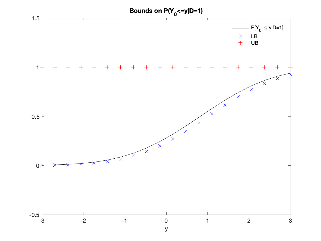
Figure 1: Bounds on $\Pr[Y_{0}\leq y|D=1]$ When $L=2$

Figure 2: Bounds on $\Pr[Y_{0}\leq y|D=1]$ When $L=5$

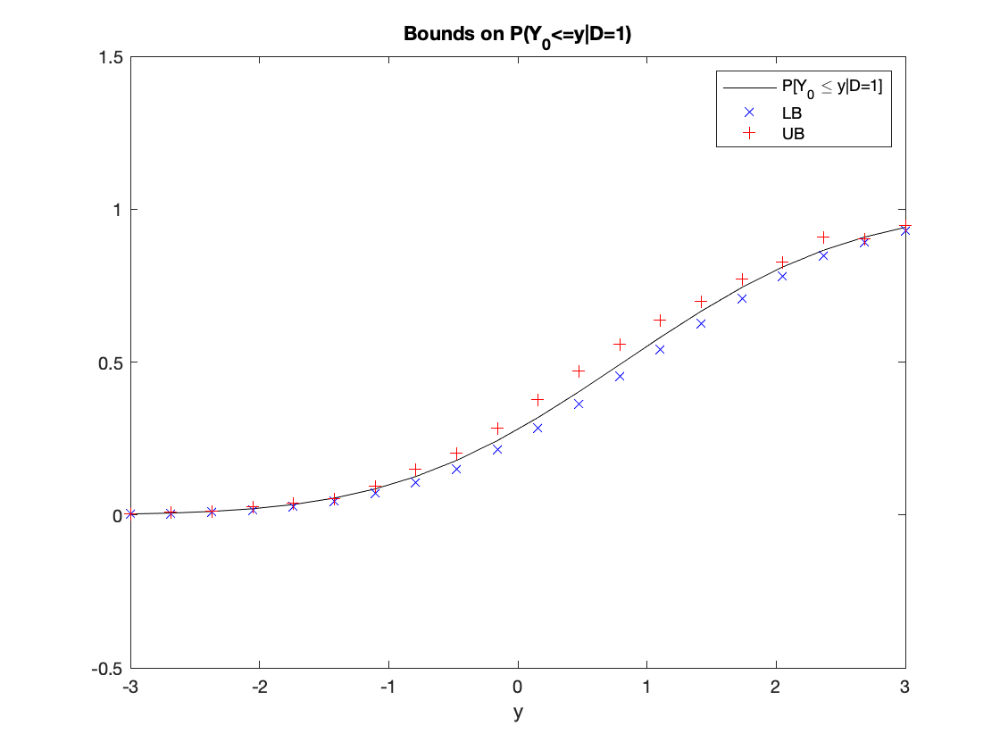
Figure 3: Bounds on $\Pr[Y_{0}\leq y|D=1]$ When $L=6$

Appendix A Point Identification

Point identification of $QTE_{\tau}(d,x)$ and $ATE(d,x)$ can be achieved as long as the stochastic dominance ordering is preserved (i.e., Condition S₁ or S₀) and instruments have sufficient variation in a specific sense. As is clear below, however, we do not require $p(z)\rightarrow 1$ or $0$ (i.e., instruments with large support). In this sense, our approach to point identification complements the approach of identification at infinity (e.g., Heckman (1990)). To see this, consider the following theorem.

Theorem A.1.

Suppose that Assumption Z and Condition S₁ hold. Fix $x\in\mathcal{X}$. For $\gamma\equiv(\gamma_{1},...,\gamma_{L})$ in $\Gamma(x)$, suppose

$$P[Y\leq\cdot|D=1,X=x]=\sum_{\ell=1}^{L}\gamma_{\ell}P[Y\leq\cdot,D=1|Z=z_{\ell},X=x].$$ (A.1)

Then $F_{Y_{0}|D,X}(\cdot|1,x)$ is identified as

$$P[Y_{0}\leq\cdot|D=1,X=x] =-\sum_{\ell=1}^{L}\gamma_{\ell}P[Y\leq\cdot,D=0|Z=z_{\ell},X=x]$$ (A.2)

The key for this point identification result is that there exists $\gamma$ such that (A.1) holds, which is a stronger requirement than the inequality version (2.3). The equation (A.1) is more likely to hold when $L$ is large, that is, when instruments take more values. In particular, when $L\rightarrow\infty$ (e.g., continuous $Z$), we may view that $P[Y\leq y|D=1,X=x]$ is approximated as

$$P[Y\leq y|D=1,X=x] =\lim_{L\rightarrow\infty}\sum_{\ell=1}^{L}\gamma_{\ell,L}p(z_{\ell},x)P[Y\leq y|D=1,Z=z_{\ell},X=x],$$

where $\sum_{\ell=1}^{L}\gamma_{\ell,L}=0$. Note that, although this does not demand an infinite support for $Z$, it implicitly assumes that $Z$ sufficiently influences the distribution of $Y$ conditional on $(D,X)=(1,x)$ in a way that the resulting functions, $P[Y\leq y|D=1,Z=z_{\ell},X=x]$, generate $P[Y\leq y|D=1,X=x]$. Importantly, whether this is possible or not can be confirmed from the data.

Given Theorem A.1, we identify $QTE_{\tau}(1,x)=Q_{Y|D,X}(\tau|1,x)-Q_{Y_{0}|D,X}(\tau|1,x)$ where $Q_{Y_{0}|D,X}(\tau|1,x)$ is a solution to $\tau=-\sum_{\ell=1}^{L}\gamma_{\ell}P[Y\leq\cdot,D=0|Z=z_{\ell},X=x]$. Similarly, under Condition S₀, we can identify $F_{Y_{0}|D,X}(\cdot|1,x)$ and thus $QTE_{\tau}(0,x)$. We omit this result for succinctness.

It is worth comparing the point identification result with that in Chernozhukov and Hansen (2005). The latter point identifies $QTE_{\tau}(x)$ with a binary instrument by assuming rank similarity. The result of this section suggests that the identification of $QTE_{\tau}(x)$ can alternatively be achieved when Conditions S₁ and S₀ both hold and the IVs satisfy (A.1). To see the connection to rank similarity, note that rank similarity implies Condition S^∗ (by Theorem 3.2), but the latter implies Conditions S₁ and S₀ that identify $QTE_{\tau}(1,x)$ and $QTE_{\tau}(0,x)$, respectively, and thus $QTE_{\tau}(x)$ jointly. In this way, the two approaches enjoy different levels of the trade-off between restrictions on the heterogeneity and exogenous variation.

Appendix B Conditions for Average Treatment Effects

To calculate bounds on $ATE(1,x)$ and $ATE(0,x)$, we introduce conditions that are weaker that Conditions S₁ and S₀.

Condition S${}_{1}^{\prime}$.

For arbitrary non-negative weight vectors $(w_{1},...,w_{L})$ and $(\tilde{w}_{1},...,\tilde{w}_{L})$ that satisfy $\sum_{\ell=1}^{L}w_{\ell}=\sum_{\ell=1}^{L}\tilde{w}_{\ell}=1$, if

$$\sum_{\ell=1}^{L}w_{\ell}P[Y_{1}\leq\cdot|D=1,Z=z_{\ell},X=x] \leq\sum_{\ell=1}^{L}\tilde{w}_{\ell}P[Y_{1}\leq\cdot|D=1,Z=z_{\ell},X=x],$$ (B.1)

then

$$\sum_{\ell=1}^{L}w_{\ell}E[Y_{0}|D=1,Z=z_{\ell},X=x] \leq\sum_{\ell=1}^{L}\tilde{w}_{\ell}E[Y_{0}|D=1,Z=z_{\ell},X=x].$$ (B.2)

Condition S${}_{1}^{\prime}$ can be used to bound the $ATE(1,x)$. An analogous condition can be imposed to bound $ATE(0,x)$.

Condition S${}_{0}^{\prime}$.

For arbitrary non-negative weight vectors $(w_{1},...,w_{L})$ and $(\tilde{w}_{1},...,\tilde{w}_{L})$ that satisfy $\sum_{\ell=1}^{L}w_{\ell}=\sum_{\ell=1}^{L}\tilde{w}_{\ell}=1$, if

$$\sum_{\ell=1}^{L}w_{\ell}P[Y_{0}\leq\cdot|D=1,Z=z_{\ell},X=x] \leq\sum_{\ell=1}^{L}\tilde{w}_{\ell}P[Y_{0}\leq\cdot|D=1,Z=z_{\ell},X=x],$$ (B.3)

then

$$\sum_{\ell=1}^{L}w_{\ell}E[Y_{1}|D=1,Z=z_{\ell},X=x] \leq\sum_{\ell=1}^{L}\tilde{w}_{\ell}E[Y_{1}|D=1,Z=z_{\ell},X=x].$$ (B.4)

Appendix C Other Structural Models as Sufficient Conditions

We present two more structural models that are not nested to Model 1 in the text. Model1(i) are maintained in these models, that is, $Y=q(D,X,U_{D})$ where $q(d,x,\cdot)$ is continuous and monotone increasing and $D=h(Z,X,\eta)$.

Model 2. (ii) $U_{0}\stackrel{{\scriptstyle d}}{{=}}\phi(U_{1},V)$ conditional on $(\eta,X)$ where $V\perp(U_{1},\eta)|X$ and $\phi(\cdot,v)$ is strictly increasing for all $v$.

Model 2(ii) defines that $U_{0}$ is “noisier” than $U_{1}$. Therefore, Model 2 is weaker than the model in Chernozhukov and Hansen (2005). Model 2 and Model 1 are not nested because, in $U_{0}=U_{1}+V$ of Model 1, $V$ is not independent of $U_{1}$. We show below that Model 2 implies Condition S₁. Interestingly, Model 2(ii) with $U_{0}=\phi(U_{1},V)$ (instead of “$\stackrel{{\scriptstyle d}}{{=}}$”) is a generalization of the definition that $U_{0}$ is “noisier” than $U_{1}$ if $U_{0}=U_{1}+V$ with $U_{1}\perp V$ in Pomatto et al. (2020, p. 1880).

Model 3. (ii) $U_{0}\stackrel{{\scriptstyle d}}{{=}}\max\{\phi(U_{1}),V\}$ conditional on $(\eta,X)$ where $V\perp(U_{1},\eta)|X$ and $\phi(\cdot)$ is strictly increasing.

We show below that Model 3 implies rank linearity. Model 3 can alternatively be defined as follows: $Y_{0}\stackrel{{\scriptstyle d}}{{=}}\max\{\phi(Y_{1}),V\}$ conditional on $(\eta,X)$ where $V\perp(Y_{1},\eta)|X$ and $\phi(\cdot)$ is strictly increasing. Then, this model also implies rank linearity with $\psi(\cdot)=\phi^{-1}(\cdot)$ because

$$\Pr[Y_{0}\leq y|\eta,X] =\Pr[\phi(Y_{1})\leq y,V\leq y|\eta,X]=\Pr[Y_{1}\leq\phi^{-1}(y)|\eta,X]\Pr[V\leq y|X].$$

This model provides another interpretation of an insurance policy ($D=1$) as $Y_{1}=\max\{Y_{0},V\}$ guarantees at least $Y_{0}$. Models 2 and 3 are not nested.

Lemma C.1.

(i) Model 2 implies Condition S${}_{1}^{*}$; (ii) Model 3 implies rank linearity.

The proof of this lemma is contained in Section E.

Appendix D Bounding Violation Probability in Linear Program with Randomized Constraints

Let $h(\gamma,y)\equiv p(y|1)-\boldsymbol{p}(y,1)^{\prime}\gamma$. Following Calafiore and Campi (2005), define a violation probability and a robustly feasible solution.

Definition D.1 (Violation probability).

Let $\gamma\in\Gamma$ be a candidate solution for (4.1)–(4.4). The probability of violation of $\gamma$ is defined as

$$V(\gamma) =\mathbb{P}\{Y\in\mathcal{Y}:h(\gamma,Y)>0\},$$

where $\{Y\in\mathcal{Y}:h(\gamma,Y)>0\}$ is assumed to be measurable.

Note that $V(\gamma^{*})=0$ where $\gamma^{*}$ is the solution to (4.1)–(4.4).

Definition D.2 ($\epsilon$-level solution).

For $\epsilon\in[0,1]$, $\gamma\in\Gamma$ is an $\epsilon$-level robustly feasible solution if $V(\gamma)\leq\epsilon$.

Then, we can show that the violation probability at the solution, denoted as $\bar{\gamma}_{n}$, to (4.3)–(4.4) is on average bounded by $1/n$.

Proposition D.1.

Let $\bar{\gamma}_{n}$ be the solution to (4.3)–(4.4). Then,

$$\mathbb{E}_{P^{n}}[V(\bar{\gamma}_{n})] \leq\frac{1}{n+1},$$

where $P^{n}$ is the probability measure in the space $\mathcal{Y}^{n}$ of the multi-sample extraction $Y_{1},...,Y_{n}$.

Corollary D.1.

Fix $\epsilon\in[0,1]$ and $\beta\in[0,1]$ and let

$$n \geq\frac{1}{\epsilon\beta}-1.$$

Then, with probability no smaller than $1-\beta$, the sampled LP (4.3)–(4.4) returns an optimal solution $\hat{\gamma}_{n}$ which is $\epsilon$-level robustly feasible.

The above results implicitly assume a particular rule of tie-breaking when there are multiple solutions in the sampled LP (see Theorem 3 in Calafiore and Campi (2005)). There is also discussions on no solution in the paper.

Appendix E Proofs

E.1 Proof of Lemma 3.1

Let $p(z,x)\equiv P[D=1|Z=z,X=x]$ and let $H(z,x)\equiv\{\eta:h(z,x,\eta)=1\}$ be a level set. Then,

$$\sum_{\ell}w_{\ell}P[Y_{1}\leq y|D=1,Z=z_{\ell},X=x] =\sum_{\ell}w_{\ell}P[Y_{1}\leq y|\eta\in H(z_{\ell},x),X=x]$$

$$=\int\frac{\sum_{\ell}w_{\ell}1[t\in H(z_{\ell},x)]}{p(z_{\ell},x)}P[Y_{1}\leq y|\eta=t,X=x]dt.$$

Take $w(t,x)=\frac{\sum_{\ell}w_{\ell}1[t\in H(z_{\ell},x)]}{p(z_{\ell},x)}$. Then, $w(t,x)$ satisfies

$$\int\frac{\sum_{\ell}w_{\ell}1[t\in H(z_{\ell},x)]}{p(z_{\ell},x)}dt =1.$$

The same argument applies to $\tilde{w}$ and $\tilde{w}(t,x)$, and also for the distribution of $Y_{0}$. $\square$

E.2 Proof of Theorem 2.1

We suppress $X$ for simplicity and prove the upper bound; the lower bound can be analogously derived. Without loss of generality, for some $\ell^{*}\leq L$, let $\gamma_{\ell}\leq 0$ for $\ell\leq\ell^{*}$ and $\gamma_{\ell}>0$ for $\ell>\ell^{*}$. Let $q(z_{\ell})\equiv P[Z=z_{\ell}|D=1]$. Then, (2.3) can be rewritten as

$$\sum_{\ell=1}^{L}q(z_{\ell})\times P[Y\leq y|D=1,Z=z_{\ell}]-\sum_{\ell=1}^{\ell^{*}}\gamma_{\ell}p(z_{\ell})\times P[Y\leq y|D=1,Z=z_{\ell}]\\ \leq\sum_{\ell=\ell^{*}+1}^{L}\gamma_{\ell}p(z_{\ell})\times P[Y\leq y|D=1,Z=z_{\ell}].$$

Let $a\equiv 1-\sum_{\ell=1}^{\ell^{*}}\gamma_{\ell}p(z_{\ell})$. By definition and that $\sum_{\ell=1}^{L}\gamma_{\ell}p(z_{\ell})=1$, we have $a=\sum_{\ell=\ell^{*}+1}^{L}\gamma_{\ell}p(z_{\ell})$. Therefore, we have

$$\sum_{\ell=1}^{\ell^{*}}\frac{q(z_{\ell})-\gamma_{\ell}p(z_{\ell})}{a}\times P[Y_{1}\leq y|D=1,Z=z_{\ell}]+\sum_{\ell=\ell^{*}+1}^{L}\frac{q(z_{\ell})}{a}\times P[Y_{1}\leq y|D=1,Z=z_{\ell}]\\ \leq\sum_{\ell=\ell^{*}+1}^{L}\frac{\gamma_{\ell}p(z_{\ell})}{a}\times P[Y_{1}\leq y|D=1,Z=z_{\ell}],$$

where $\sum_{\ell=1}^{\ell^{*}}\frac{q(z_{\ell})-\gamma_{\ell}p(z_{\ell})}{a}+\sum_{\ell=\ell^{*}+1}^{L}\frac{q(z_{\ell})}{a}=1$ and $\sum_{\ell=\ell^{*}+1}^{L}\frac{\gamma_{\ell}p(z_{\ell})}{a}=1$. Therefore, by Condition S₁, we have

$$\sum_{\ell=1}^{k}\frac{q(z_{\ell})-\gamma_{\ell}p(z_{\ell})}{a}\times P[Y_{0}\leq y|D=1,Z=z_{\ell}]+\sum_{\ell=\ell^{*}+1}^{L}\frac{q(z_{\ell})}{a}\times P[Y_{0}\leq y|D=1,Z=z_{\ell}]\\ \leq\sum_{\ell=\ell^{*}+1}^{L}\frac{\gamma_{\ell}p(z_{\ell})}{a}\times P[Y_{0}\leq y|D=1,Z=z_{\ell}].$$

Equivalently, we have

$$P[Y_{0}\leq y|D=1] \leq \sum_{\ell=1}^{L}\gamma_{\ell}\times P[Y_{0}\leq y,D=1|Z=z_{\ell}]$$

$$= \sum_{\ell=1}^{L}\gamma_{\ell}\times\left\{P[Y_{0}\leq y|Z=z_{\ell}]-P[Y_{0}\leq y,D=0|Z=z_{\ell}]\right\}$$

$$= \sum_{\ell=1}^{L}\gamma_{\ell}P[Y_{0}\leq y|Z=z_{\ell}]-\sum_{\ell=1}^{L}\gamma_{\ell}\times P[Y_{0}\leq y,D=0|Z=z_{\ell}]$$

$$= P[Y_{0}\leq y]\times\sum_{\ell=1}^{L}\gamma_{\ell}-\sum_{\ell=1}^{L}\gamma_{\ell}\times P[Y\leq y,D=0|Z=z_{\ell}]$$

$$= -\sum_{\ell=1}^{L}\gamma_{\ell}\times P[Y\leq y,D=0|Z=z_{\ell}],$$

where the last equality is by $\sum_{\ell=1}^{L}\gamma_{\ell}=0$. $\square$

E.3 Proof of Lemma 2.1

Note that $P[Y_{d}\leq y|D_{z_{1}}=1]=P[Y_{d}\leq y|\text{AT}]$ and, for $\ell=\{2,...,L\}$,

$$P[Y_{d}\leq y|D_{z_{\ell}}=1] =\frac{1}{p(z_{\ell})}P\left[Y_{d}\leq y,\{\text{AT}\}\cup\bigcup_{\ell^{\prime}=2}^{\ell}\{(z_{\ell^{\prime}-1},z_{\ell^{\prime}})\text{-C}\}\right]$$

by Assumption LABEL:as:D* and $p(z_{\ell})=P[D_{z_{\ell}}=1]$. Then, in (2.13),

$$\sum_{\ell=1}^{L}w_{\ell}P[Y_{d}\leq y|D_{z_{\ell}}=1]$$

$$=w_{1}P[Y_{d}\leq y|\text{AT}]+\sum_{\ell=2}^{L}\frac{w_{\ell}}{p(z_{\ell})}\left(p_{1}P[Y_{d}\leq y|\text{AT}]+\sum_{\ell^{\prime}=2}^{\ell}p_{\ell^{\prime}}P[Y_{d}\leq y|(z_{\ell^{\prime}-1},z_{\ell^{\prime}})\text{-C}]\right)$$

and similarly for the right-hand side of (2.13). This proves (i). To remove the distributions for AT in the expressions, we set

$$w_{1}+p_{1}\sum_{\ell=2}^{L}\frac{w_{\ell}}{p(z_{\ell})} =\tilde{w}_{1}+p_{1}\sum_{\ell=2}^{L}\frac{\tilde{w}_{\ell}}{p(z_{\ell})}.$$ (E.1)

Then, note that when $L\geq 2$, $w\neq\tilde{w}$ even if $w$ and $\tilde{w}$ satisfy (E.1). Therefore, the resulting (2.13) is the dominance between the two distinct weight sums of $P[Y_{d}\leq y|(z_{\ell^{\prime}-1},z_{\ell^{\prime}})\text{-C}]$’s:

$$\sum_{\ell=2}^{L}\frac{w_{\ell}}{\sum_{\ell^{\prime}=1}^{\ell}p_{\ell^{\prime}}}\sum_{\ell^{\prime}=2}^{\ell}p_{\ell^{\prime}}P[Y_{d}\leq y|(z_{\ell^{\prime}-1},z_{\ell^{\prime}})\text{-C}] \leq\sum_{\ell=2}^{L}\frac{\tilde{w}_{\ell}}{\sum_{\ell^{\prime}=1}^{\ell}p_{\ell^{\prime}}}\sum_{\ell^{\prime}=2}^{\ell}p_{\ell^{\prime}}P[Y_{d}\leq y|(z_{\ell^{\prime}-1},z_{\ell^{\prime}})\text{-C}],$$

which can be simplified as (2.15) in (ii). $\square$

E.4 Proof of Theorem 3.1

We suppress $X$ for simplicity. For an arbitrary r.v. $A$, let $F_{A}^{w}(\cdot)\equiv\int w(t)F_{A|\eta}(\cdot|t)dt$, which itself is a CDF. By (3.2) in Model 1(i), $F_{Y_{d}}^{w}\leq F_{Y_{d}}^{\tilde{w}}$ if and only if $F_{U_{d}}^{w}\leq F_{U_{d}}^{\tilde{w}}$ . So it suffices to show that, if $F_{U_{1}}^{w}\leq F_{U_{1}}^{\tilde{w}}$, then $F_{U_{0}}^{w}\leq F_{U_{0}}^{\tilde{w}}$.

Let $G(\cdot)$ be an arbitrary monotone increasing function and $g(\cdot)\equiv G^{\prime}(\cdot)$. Note that

$$\int GdF_{U_{0}}^{w}-\int GdF_{U_{0}}^{\tilde{w}}=\int[\int\tilde{w}(t)F_{U_{0}|\eta}(u|t)dt-\int w(t)F_{U_{0}|\eta}(u|t)dt]g(u)du$$

$$=\int[\int\tilde{w}(t)\int F_{U|\eta}(u-s|t)f_{\xi_{0}}(s)dsdt-\int w(t)\int F_{U|\eta}(u-s|t)f_{\xi_{0}}(s)dsdt]g(u)du$$

$$=\int\int\int[\tilde{w}(t)-w(t)]F_{U|\eta}(u|t)f_{\xi_{0}}(s)g(u+s)dudsdt,$$

where the first eq. is due to the integration by part, the second eq. is by $F_{U_{d}|\eta}(u|t)=\int F_{U|\eta}(u-s|t)f_{\xi_{0}|\eta}(s|t)ds=\int F_{U|\eta}(u-s|t)f_{\xi_{0}}(s)ds$ under Model 1(ii), and the last eq. is by change of variables. By Model 1(iii), $f_{\xi_{0}}(s)=\int f_{\xi_{1}}(s-v)f_{V}(v)dv=\int f_{\xi_{1}}(v)f_{V}(s-v)dv$ where $f_{A}(\cdot)$ is the PDF of an arbitrary r.v. $A$. Therefore,

$$\int GdF_{U_{0}}^{w}-\int GdF_{U_{0}}^{\tilde{w}}$$

$$=\int\int\int[\tilde{w}(t)-w(t)]F_{U|\eta}(u|t)\int f_{\xi_{1}}(v)f_{V}(s-v)g(u+s)dvdudsdt$$

$$=\int\int[\tilde{w}(t)-w(t)]F_{U|\eta}(u|t)\int f_{\xi_{1}}(v)[\int f_{V}(s)g(u+s+v)ds]dvdudt.$$

Let $\psi(s)\equiv\int f_{V}(t)g(t+s)dt$. By definition, $\psi\geq 0$ since $g\geq 0$. Therefore,

$$\int GdF_{U_{0}}^{w}-\int GdF_{U_{0}}^{\tilde{w}}$$

$$=\int\int[\tilde{w}(t)-w(t)]F_{U|\eta}(u|t)\int f_{\xi_{1}}(v)\psi(u+v)dvdudt$$

$$=\int\int[\tilde{w}(t)-w(t)]\int F_{U|\eta}(u-v|t)f_{\xi_{1}}(v)dv\psi(u)dudt$$

$$=\int\int[\tilde{w}(t)-w(t)]\int F_{U_{1}|\eta}(u|t)\psi(u)dudt$$

$$=\int[\int\tilde{w}(t)F_{U_{1}|\eta}(u|t)dt-\int w(t)F_{U_{1}|\eta}(u|t)dt]\psi(u)du\geq 0,$$

where the last ineq. is by $F_{U_{1}}^{w}\leq F_{U_{1}}^{\tilde{w}}$. Because $G(\cdot)$ is arbitrary, then $F_{U_{0}}^{w}$ is first order stochastic dominant over $F_{U_{0}}^{\tilde{w}}$. $\square$

E.5 Proof of Theorem 3.3: Equivalence Between Rank Linearity and Condition S^∗

The “if” part is trivial. We prove “only if” part. Suppress $(Z,X)$ for simplicity. Suppose Condition S^∗ holds. Let $\mathcal{Y}_{\infty}\equiv\{y_{k}\in\mathbb{R}:k=1,\cdots,\infty\}$ be a sequence that is dense on $\mathbb{R}$. Denote $\mathcal{Y}_{n}\equiv\{y_{k}\in\mathbb{R}:k=1,\cdots,n\}$. Because $\mathcal{Y}_{\infty}$ is dense in $\mathbb{R}$ and CDFs are right-continuous, it suffices to show the existence of $\lambda(\cdot)$ and $\psi(\cdot)$ on $\mathcal{Y}_{\infty}$ such that

$$F_{Y_{0}|\eta}(\psi(y)|t)=\lambda(y)F_{Y_{1}|\eta}(y|t)$$ (E.2)

holds for all $t\in\mathcal{T}$ and $y\in\mathcal{Y}_{\infty}$.

Fix $n\in\mathbb{N}$. Let $G_{1,k}:\mathbb{R}\rightarrow\{0,1\}$ be a simple function defined as $G_{1,k}(\cdot)\equiv 1\{y_{k}\leq\cdot\}$ for $k=1,\cdots,n$. By the full rank condition (3.4), for each $1\leq k\leq n$, there exists a function $c_{k}:\mathcal{T}\rightarrow\mathbb{R}$ such that

$$G_{1,k}(\cdot)=\int c_{k}(t)F_{Y_{1}|\eta}(\cdot|t)dt.$$

Define $G_{0,k}:\mathbb{R}\rightarrow[0,1]$ as

$$G_{0,k}(\cdot)\equiv\int c_{k}(t)F_{Y_{0}|\eta}(\cdot|t)dt.$$

Note that $G_{0,k}$ is a proper CDF. Now, for any vectors $\pi\equiv(\pi_{1},\cdots,\pi_{n})$ and $\tilde{\pi}\equiv(\tilde{\pi}_{1},\cdots,\tilde{\pi}_{n})$ such that $\sum_{k=1}^{n}\pi_{k}=\sum_{k=1}^{n}\tilde{\pi}_{k}=1$, suppose

$$\sum_{k=1}^{n}\pi_{k}G_{1,k}(\cdot)\leq\sum_{k=1}^{n}\tilde{\pi}_{k}G_{1,k}(\cdot).$$

It follows that

$$\int b_{n}(t)F_{Y_{1}|\eta}(\cdot|t)dt\leq\int\tilde{b}_{n}(t)F_{Y_{1}|\eta}(\cdot|t)dt,$$

where $b_{n}(t)\equiv\sum_{k=1}^{n}\pi_{k}c_{k}(t)$ and $\tilde{b}_{n}(t)\equiv\sum_{k=1}^{n}\tilde{\pi}_{k}c_{k}(t)$. Let $b_{n}^{+}(t)=\max\{b_{n}(t),0\}$ and $b_{n}^{-}(t)=\min\{b_{n}(t),0\}$ and similarly define $\tilde{b}_{n}^{+}(t)$ and $\tilde{b}_{n}^{-}(t)$. Then, the above inequality can be written as

$$\int\{b_{n}^{+}(t)-\tilde{b}_{n}^{-}(t)\}F_{Y_{1}|\eta}(\cdot|t)dt\leq\int\{\tilde{b}_{n}^{+}(t)-b_{n}^{-}(t)\}F_{Y_{1}|\eta}(\cdot|t)dt,$$

where the resulting weight functions on both sides are non-negative. Then, by Condition S^∗, we have

$$\sum_{k=1}^{n}\pi_{k}G_{0,k}(\cdot)\leq\sum_{k=1}^{n}\tilde{\pi}_{k}G_{0,k}(\cdot)$$

By a similar argument, the converse is also true and thus we have

$$\sum_{k=1}^{n}\pi_{k}G_{1,k}(\cdot)\leq\sum_{k=1}^{n}\tilde{\pi}_{k}G_{1,k}(\cdot).$$

if and only if

$$\sum_{k=1}^{n}\pi_{k}G_{0,k}(\cdot)\leq\sum_{k=1}^{n}\tilde{\pi}_{k}G_{0,k}(\cdot)$$

for any non-negative weights $\pi$ and $\tilde{\pi}$. Therefore, it follows that

$$\sum_{k=1}^{n}\delta_{k}G_{1,k}(\cdot)\leq 0\text{ if and only if }\sum_{k=1}^{n}\delta_{k}G_{0,k}(\cdot)\leq 0$$ (E.3)

for any $n$-dimensional vector $\delta\equiv(\delta_{1},\cdots,\delta_{n})$ that satisfies $\sum_{k=1}^{n}\delta_{k}=0$.

For $d\in\{0,1\}$, define

$$\Delta_{d}^{G} \equiv\left\{\delta\in\mathbb{R}^{n}:\sum_{k=1}^{n}\delta_{k}G_{d,k}(y)\leq 0\text{ }\forall y\in\mathbb{R};\sum_{k=1}^{n}\delta_{k}=0\right\}.$$

Note that $\{\big{(}G_{1,1}(y),\cdots,G_{1,n}(y)\big{)}:y\in\mathbb{R}\}=\{\big{(}G_{1,1}(y),\cdots,G_{1,n}(y)\big{)}:y\in\mathcal{Y}_{n}\}$ by definition. Therefore, $\Delta_{1}^{G}$ is a finite cone and its dimension is $n-1$. Define the polar cone of $\Delta_{d}^{G}$ as $\Delta_{d}^{G*}\equiv\{G_{d}\in\mathbb{R}^{n}:G_{d}^{\prime}\delta\leq 0,\forall\delta\in\Delta_{d}^{G}\}$. Note that by definition, $\big{(}G_{1,1}(y),\cdots,G_{1,n}(y)\big{)}$ for $y\in\mathcal{Y}_{n}/\{y_{n}\}$ are $n-1$ linearly independent vectors and therefore generate extreme rays of $\Delta_{1}^{G*}$. Also note that any element in $\Delta_{0}^{G*}$ is written as $\big{(}G_{0,1}(y),\cdots,G_{0,n}(y)\big{)}$ for some $y\in\mathbb{R}$, and so is a vector that generates its extreme ray. But by (E.3), we have that $\Delta_{1}^{G}=\Delta_{0}^{G}$ and thus $\Delta_{1}^{G*}=\Delta_{0}^{G*}$, and therefore, for each $y_{k}\in\mathcal{Y}_{n}/\{y_{n}\}$, there exists $y_{k}^{*}\in\mathbb{R}$ and $\lambda_{n}(\cdot)>0$ such that

$$\big{(}G_{0,1}(y_{k}^{*}),\cdots,G_{0,n}(y_{k}^{*})\big{)}=\lambda_{n}(y_{k})\times\big{(}G_{1,1}(y_{k}),\cdots,G_{1,n}(y_{k})\big{)}.$$ (E.4)

If there exists multiple values of $y_{k}^{*}$ satisfying (E.4), we define $y_{k}^{*}$ as the infimum of $\{\tilde{y}_{k}^{*}:\big{(}G_{0,1}(\tilde{y}_{k}^{*}),\cdots,G_{0,n}(\tilde{y}_{k}^{*})\big{)}=\lambda_{n}(y_{k})\times\big{(}G_{1,1}(y_{k}),\cdots,G_{1,n}(y_{k})\big{)}\}$. Because CDFs are right-continuous function, the infimum should also satisfy (E.4).

For any $j,k=1,...,n$, if $G_{1,j}(y_{k})=0$ then $G_{0,j}(y_{k}^{*})=0$ by (E.4), which further implies that $G_{0,j}(y^{*})=0$ for all $y^{*}\leq y_{k}^{*}$ because $G_{0,j}(\cdot)$ is monotone increasing. Let $\{j_{1},\cdots,j_{n}\}$ be a permutation of $\{1,\cdots,n\}$ such that $y_{j_{1}}<y_{j_{2}}<\cdots<y_{j_{n}}$. Note that $G_{1,j_{1}}(y_{j_{1}})$ is the only non-zero component in the set $\{G_{1,k}(y_{j_{1}}):k=1,\cdots,n\}$. Then, by (E.4), $G_{0,j_{1}}(y_{j_{1}}^{*})\neq 0$ and $G_{0,j_{k}}(y_{j_{1}}^{*})=0$ for $k\geq 2$. Similarly, there are two elements of $\{G_{0,k}(y_{j_{2}}^{*}):k=1,\cdots,n\}$ which are non-zero, namely, $G_{0,j_{1}}(y_{j_{2}}^{*})$ and $G_{0,j_{2}}(y_{j_{2}}^{*})$. Therefore, by $G_{0,j_{2}}(y_{j_{1}}^{*})=0$ and $G_{0,j_{2}}(y_{j_{2}}^{*})\neq 0$ and the fact that $G_{0,j_{2}}(\cdot)$ is monotone increasing, we can conclude $y_{j_{1}}^{*}<y_{j_{2}}^{*}$. Continuing this argument, we can conclude that

$$y_{j_{1}}^{*}<y_{j_{2}}^{*}<\cdots<y_{j_{n}}^{*}.$$

Define a function $\psi_{n}:y_{k}\mapsto y_{k}^{*}$ for $k=1,\cdots,n$. By the above analysis, $\psi_{n}(\cdot)$ is a monotone increasing function. Note that the support of $\psi_{n}$ is $\mathcal{Y}_{n}$, which we extend to $\mathbb{R}$ as follows: for any $y\in\mathbb{R}$,

$$\psi_{n}(y)=\left\{\begin{array}[]{cc}\max\{\psi_{n}(y_{k}):y_{k}\leq y,\text{ }k=1,\cdots,n\}&\text{ if }y\geq\min\{y_{1},\cdots,y_{n}\}\\ -\infty&\text{otherwise}\end{array}\right.$$

Then, $\psi_{n}:\mathbb{R}\rightarrow\mathbb{R}$ is still a monotone increasing function.

We now consider increasing $n$ to $n+1$. By a similar argument, there exists a sequence $\{y_{1}^{\dagger},\cdots,y_{n}^{\dagger},y_{n+1}^{\dagger}\}$ and $\lambda_{n+1}(\cdot)>0$ such that for $k=1,\cdots,n+1$, we have

$$\big{(}G_{0,1}(y_{k}^{\dagger}),\cdots,G_{0,n}(y_{k}^{\dagger}),G_{0,n+1}(y_{k}^{\dagger})\big{)}=\lambda_{n+1}(y_{k})\times\big{(}G_{1,1}(y_{k}),\cdots,G_{1,n}(y_{k}),G_{1,n+1}(y_{k})\big{)},$$ (E.5)

If there exists multiple values of $y_{k}^{\dagger}$, we define $y_{k}^{\dagger}$ as the infimum of them. Note that, by (E.5) and (E.4), $y_{k}^{\dagger}$ is one of the candidates $\tilde{y}_{k}^{*}$’s that make $\big{(}G_{0,1}(\tilde{y}_{k}^{*}),\cdots,G_{0,n}(\tilde{y}_{k}^{*})\big{)}$ proportional to $\big{(}G_{1,1}(y_{k}),\cdots,G_{1,n}(y_{k})\big{)}$ satisfy (E.4). While $y_{k}^{*}$ is the infimum of those candidates, $y_{k}^{\dagger}$ cannot reach that infimum because it has to satisfies the additional restriction, $G_{0,n+1}(y_{k}^{\dagger})=\lambda_{n+1}(y_{k})G_{1,n+1}(y_{k})$. Therefore, we can conclude that $y_{k}^{\dagger}\geq y_{k}^{*}$ for $k=1,\cdots,n$. Using $\{y_{1},\cdots,y_{n},y_{n+1}\}$ and $\{y_{1}^{\dagger},\cdots,y_{n}^{\dagger},y_{n+1}^{\dagger}\}$, define $\psi_{n+1}(\cdot)$ analogous to $\psi_{n}(\cdot)$ above. Then, $\psi_{n+1}(y_{k})=y_{k}^{\dagger}\geq y_{k}^{*}=\psi_{n}(y_{k})$ for $k=1,\cdots,n$. Furthermore, by definition, $\psi_{n+1}(y_{n+1})\geq\psi_{n}(y_{n+1})$ regardless of the rank order of $y_{n+1}$ in $\mathcal{Y}_{n+1}$. Therefore, for any $y\in\mathbb{R}$,

$$\psi_{n+1}(y)\geq\psi_{n}(y),$$

and thus the limit of the sequence of functions $\psi_{n}(\cdot)$ exists as $n\rightarrow\infty$, which we denote as $\psi_{\infty}(\cdot)$. Recall each $\psi_{n}(\cdot)$ is weakly increasing. It is easy to prove by contradiction that $\psi_{\infty}(\cdot)$ is strictly increasing. Fix $y_{k}\in\mathcal{Y}_{\infty}$. For any $n\geq k$, $\big{(}G_{0,1}(\psi_{\infty}(y_{k})),\cdots,G_{0,n}(\psi_{\infty}(y_{k}))\big{)}$ is proportional to $\big{(}G_{1,1}(y_{k}),\cdots,G_{1,n}(y_{k})\big{)}$ and therefore there exists $\lambda_{\infty}(y_{k})$ such that

$$\big{(}G_{0,1}(\psi_{\infty}(y_{k})),\cdots,G_{0,n}(\psi_{\infty}(y_{k}))\big{)}=\lambda_{\infty}(y_{k})\times\big{(}G_{1,1}(y_{k}),\cdots,G_{1,n}(y_{k})\big{)}$$ (E.6)

for any $n\in\mathbb{N}$. Moreover, because $\mathcal{Y}_{\infty}$ is dense in $\mathbb{R}$ and $\psi_{\infty}$ and $G_{d,k}$ are right-continuous functions, the above condition holds for all $y\in\mathbb{R}$.

Note $\{G_{1,k}(\cdot):k=1,\cdots,\infty\}$ is a class of simple functions. Therefore, any $F_{Y_{1}|\eta}(\cdot|t)$ can be written as

$$F_{Y_{1}|\eta}(\cdot|t)=\lim_{K\rightarrow\infty}\sum_{k=1}^{K}a_{K,k}(t)G_{1,k}(\cdot)$$

for some triangular array $\{a_{Kk}(t):1\leq k\leq K,K=1,2,\cdots,\infty\}$. By the definition of $G_{1,k}(\cdot)$, it follows that

$$F_{Y_{1}|\eta}(\cdot|t) =\lim_{K\rightarrow\infty}\sum_{k=1}^{K}a_{K,k}(t)\int w_{k}(s)F_{Y_{1}|\eta}(\cdot|s)ds=\int\lim_{K\rightarrow\infty}\sum_{k=1}^{K}a_{K,k}(t)w_{k}(s)F_{Y_{1}|\eta}(\cdot|s)ds$$

$$\equiv\int\kappa(t,s)F_{Y_{1}|\eta}(\cdot|s)ds,$$ (E.7)

where $\kappa(t,s)\equiv\lim_{K\rightarrow\infty}\sum_{k=1}^{K}a_{K,k}(t)w_{k}(s)$ serves as a Dirac delta function. Because $F_{Y_{1}|\eta}(\cdot|t)=\int\kappa(t,s)F_{Y_{1}|\eta}(\cdot|s)ds$ if and only if $F_{Y_{1}|\eta}(\cdot|t)\leq\int\kappa(t,s)F_{Y_{1}|\eta}(\cdot|s)ds$ and $F_{Y_{1}|\eta}(\cdot|t)\geq\int\kappa(t,s)F_{Y_{1}|\eta}(\cdot|s)ds$, we have, by Condition S^∗,

$$F_{Y_{0}|\eta}(\cdot|t)=\int\kappa(t,s)F_{Y_{0}|\eta}(\cdot|s)ds=\lim_{K\rightarrow\infty}\sum_{k=1}^{K}a_{K,k}(t)G_{0,k}(\cdot)$$ (E.8)

using the definition of $G_{0,k}(\cdot)$. Combining (E.7), (E.8) and (E.6), for any $y\in\mathbb{R}$ and $t\in\mathcal{T}$, we have

$$F_{Y_{0}|\eta}(\psi_{\infty}(y)|t) =\lim_{K\rightarrow\infty}\sum_{k=1}^{K}a_{K,k}(t)G_{0,k}(\psi_{\infty}(y))=\lim_{K\rightarrow\infty}\sum_{k=1}^{K}a_{K,k}(t)\lambda_{\infty}(y)G_{1,k}(y)$$

$$=\lambda_{\infty}(y)F_{Y_{1}|\eta}(y|t),$$

which completes the proof. $\boxempty$

E.6 Equivalence Between Rank Linearity and Condition S^∗: Discrete $Y_{d}$

For $d\in\{0,1\}$, suppose $Y_{d}$ and $\eta$ are discretely distributed. Specifically, let $\mathcal{Y}_{d}\equiv\big{\{}y_{d,1},\cdots,y_{d,K_{d}}\big{\}}$ and $\mathcal{T}\equiv\{t_{1},\cdots,t_{K_{\eta}}\}$ be the support of $Y_{d}$ and $\eta$, respectively. Note that even with $K_{0}=K_{1}$, we allow that $Y_{0}$ and $Y_{1}$ have different supports (i.e., allowing for a “drift”). Suppress $(Z,X)$ for simplicity.

Condition E.1.

For arbitrary non-negative weights $\{w_{1},\cdots,w_{K_{\eta}}\}$ and $\{\tilde{w}_{1},\cdots,\tilde{w}_{K_{\eta}}\}$ such that $\sum_{k=1}^{K_{\eta}}w_{k}=1$ and $\sum_{k=1}^{K_{\eta}}\tilde{w}_{k}=1$, it holds that

$$\sum_{k=1}^{K_{\eta}}w_{k}F_{Y_{1}|\eta}(\cdot|t_{k})\leq\sum_{k=1}^{K_{\eta}}\tilde{w}_{k}F_{Y_{1}|\eta}(\cdot|t_{k})$$

if and only if

$$\sum_{k=1}^{K_{\eta}}w_{k}F_{Y_{0}|\eta}(\cdot|t_{k})\leq\sum_{k=1}^{K_{\eta}}\tilde{w}_{k}F_{Y_{0}|\eta}(\cdot|t_{k}).$$

This condition can be motivated by the discussion in Remark 2.2.

Theorem E.1.

For any probability distribution function $\tilde{F}_{d}$ supported on $\mathcal{Y}_{d}\equiv\{y_{d,1},\cdots,y_{d,K_{d}}\}$, suppose there always exists a sequence $\{c_{d,1},\cdots,c_{d,K_{\eta}}\}$ such that

$$\tilde{F}_{d}(\cdot)=\sum_{k=1}^{k_{\eta}}c_{d,k}F_{Y_{d}|\eta}(\cdot|t_{k}),$$ (E.9)

Then, Condition E.1 holds if and only if (i) $K_{0}=K_{1}$ and (ii) for some strictly increasing mapping $\psi:\{y_{0,1},\cdots,y_{0,K_{0}}\}\rightarrow\{y_{1,1},\cdots,y_{1,K_{1}}\}$ and some $\lambda:\{y_{0,1},\cdots,y_{0,K_{0}}\}\rightarrow\mathbb{R}_{+}$,

$$F_{Y_{0}|\eta}(y|t_{k})=\lambda(y)F_{Y_{1}|\eta}(\psi(y)|t_{k}),\qquad\text{for }y\in\mathcal{Y}_{0},k=1,\cdots,K_{\eta}.$$ (E.10)

The condition (E.9) is a rank condition as the rank of matrix $\{F_{Y_{d}|\eta}(y_{d,j}|t_{j^{\prime}}):j=1,...,K_{d},\quad j^{\prime}=1,\cdots,k_{\eta}\}$ should be no smaller than $K_{d}$. A necessary condition is $K_{\eta}\geq K_{d}$, namely, the support of $\eta$ is no coarser than the support of $Y_{d}$. The rank condition would be violated when there is no endogeneity (i.e., $Y_{d}\perp\eta$), which is not our focus. Again, the rank condition is only introduced in this theorem to establish the relationship between rank linearity (and hence rank similarity) and the range of identifying conditions of this paper, and it is not necessary for our bound analysis.

Proof.

By Condition E.1, we have

$$\sum_{k=1}^{K_{\eta}}\delta_{k}F_{Y_{1}|\eta}(\cdot|t_{k})\leq 0\text{ if and only if }\sum_{k=1}^{K_{\eta}}\delta_{k}F_{Y_{0}|\eta}(\cdot|t_{k})\leq 0$$ (E.11)

for any $K_{\eta}$-dimensional vector $\delta\equiv(\delta_{1},\cdots,\delta_{n})$ that satisfies $\sum_{k=1}^{K_{\eta}}\delta_{k}=0$.

Note that $\big{(}F_{Y_{1}|\eta}(y|t_{1}),\cdots,(F_{Y_{1}|\eta}(y|t_{K_{\eta}})\big{)}$ for each $y\in\mathcal{Y}_{1}/\{y_{K_{1}}\}$ generates an extreme ray of the $(K_{\eta}-1)$-dimensional polar cone of a cone

$$\left\{\delta\in\mathbb{R}^{n}:\sum_{k=1}^{K_{\eta}}\delta_{k}F_{Y_{1}|\eta}(\cdot|t_{k})\leq 0;\sum_{k=1}^{K_{\eta}}\delta_{k}=0\right\}.$$

A similar argument holds for $\big{(}F_{Y_{0}|\eta}(\cdot|t_{1}),\cdots,(F_{Y_{0}|\eta}(\cdot|t_{K_{\eta}})\big{)}$. By (E.11), these two polar cones are the same. Therefore, for each $y_{k}\in\mathcal{Y}_{1}/\{y_{K_{1}}\}$, there exists a $y_{k}^{*}\in\mathcal{Y}_{0}/\{y_{K_{0}}\}$ such that

$$\big{(}F_{Y_{0}|\eta}(y_{k}^{*}|t_{1}),\cdots,F_{Y_{0}|\eta}(y_{k}^{*}|t_{K_{0}}))\big{)}=\lambda(y_{k})\times\big{(}F_{Y_{1}|\eta}(y_{k}|t_{1}),\cdots,F_{Y_{1}|\eta}(y_{k}|t_{K_{1}}))\big{)}.$$

Finally it is easy to show that if $y_{k}<y_{k^{\prime}}$ then $y_{k}^{*}<y_{k^{\prime}}^{*}$ and thus $\psi(y_{k})=y_{k}^{*}$ is a strictly increasing function.

E.7 Proof of Theorem A.1

We suppress $X$ for simplicity. The proof is analogous to that of Theorem 2.1. Using the same notation as the earlier proof, (A.1) can be rewritten as

$$\sum_{\ell=1}^{\ell^{*}}\frac{q(z_{\ell})-\gamma_{\ell}p(z_{\ell})}{a}\times P[Y_{1}\leq y|D=1,Z=z_{\ell}]+\sum_{\ell=\ell^{*}+1}^{L}\frac{q(z_{\ell})}{a}\times P[Y_{1}\leq y|D=1,Z=z_{\ell}]\\ =\sum_{\ell=\ell^{*}+1}^{L}\frac{\gamma_{\ell}p(z_{\ell})}{a}\times P[Y_{1}\leq y|D=1,Z=z_{\ell}].$$

The above equation being satisfied as equality can be viewed as being satisfied as inequalities “$\leq$” and “$\geq$.” Therefore, by Condition S₁ applied for both inequalities, we have

$$\sum_{\ell=1}^{k}\frac{q(z_{\ell})-\gamma_{\ell}p(z_{\ell})}{a}\times P[Y_{0}\leq y|D=1,Z=z_{\ell}]+\sum_{\ell=\ell^{*}+1}^{L}\frac{q(z_{\ell})}{a}\times P[Y_{0}\leq y|D=1,Z=z_{\ell}]\\ =\sum_{\ell=\ell^{*}+1}^{L}\frac{\gamma_{\ell}p(z_{\ell})}{a}\times P[Y_{0}\leq y|D=1,Z=z_{\ell}].$$

Equivalently, we have

$$P[Y_{0}\leq y|D=1] =P[Y_{0}\leq y]\times\sum_{\ell=1}^{L}\gamma_{\ell}-\sum_{\ell=1}^{L}\gamma_{\ell}\times P[Y\leq y,D=0|Z=z_{\ell}]$$

$$=-\sum_{\ell=1}^{L}\gamma_{\ell}\times P[Y\leq y,D=0|Z=z_{\ell}]$$

by $\sum_{\ell=1}^{L}\gamma_{\ell}=0$. $\square$

E.8 Proof of Lemma C.1

Part (i) can be shown analogous to the proof of Theorem 3.1. Suppose

$$\int w(t,x)F_{Y_{1}|\eta,X}(\cdot|t,x)dt\leq\int\tilde{w}(t,x)F_{Y_{1}|\eta,X}(\cdot|t,x)dt$$

holds for some $w$ and $\tilde{w}$. We want to show that

$$\int w(t,x)F_{Y_{0}|\eta,X}(\cdot|t,x)dt\leq\int\tilde{w}(t,x)F_{Y_{0}|\eta,X}(\cdot|t,x)dt.$$

First, because of the strict monotonicity of $q(d,x,\cdot)$, we have

$$\int w(t,x)F_{U_{1}|\eta,X}(\cdot|t,x)dt\leq\int\tilde{w}(t,x)F_{U_{1}|\eta,X}(\cdot|t,x)dt$$

and it suffices to show

$$\int w(t,x)F_{U_{0}|\eta,X}(\cdot|t,x)dt\leq\int\tilde{w}(t,x)F_{U_{0}|\eta,X}(\cdot|t,x)dt.$$

Second, for any $v\in\text{Supp}(V|X=x)$, because of the strict monotonicity of $\phi(\cdot,v)$, we have $1(U_{1}\leq u_{1})\overset{a.s.}{=}1(\phi(U_{1},v)\leq\phi(u_{1},v))$. Because $V\bot(U_{1},\eta)|X$, we have

$$\int w(t,x)F_{\phi(U_{1},V)|\eta,X,V}(\phi(\cdot,v)|t,x,v)dt\leq\int\tilde{w}(t,x)F_{\phi(U_{1},V)|\eta,X,V}(\phi(\cdot,v)|t,x,v)dt$$

and thus,

$$\int w(t,x)F_{U_{0}|\eta,X,V}(\phi(\cdot,v)|t,x,v)dt\leq\int\tilde{w}(t,x)F_{U_{0}|\eta,X,V}(\phi(\cdot,v)|t,x,v)dt.$$

Conditional on $(\eta,X,V)$, $\text{Supp}(\phi(U_{1},v))=\text{Supp}(\phi(U_{1},V))=\text{Supp}(U_{0})$. Therefore, for $u_{0}$ in that support,

$$\int w(t,x)F_{U_{0}|\eta,X,V}(u_{0}|t,x,v)dt\leq\int\tilde{w}(t,x)F_{U_{0}|\eta,X,V}(u_{0}|t,x,v)dt.$$

It follows that

$$\int\int w(t,x)F_{U_{0}|\eta,X,V}(u_{0}|t,x,v)f_{V|X}(v|x)dtdv$$

$$\leq \int\int\tilde{w}(t,x)F_{U_{0}|\eta,X,V}(u_{0}|t,x,v)f_{V|X}(v|x)dtdv$$

Note that $f_{V|X}=f_{V|\eta,X}$. Then, by the law of iterated expectation, we have

$$\int w(t,x)F_{U_{0}|\eta,X}(u_{0}|t,x)dt\leq\int\tilde{w}(t,x)F_{U_{0}|\eta,X}(u_{0}|t,x)dt.$$

Next, we prove part (ii) by first noting that

$$\Pr[U_{0}\leq u|\eta,X] =\Pr[\phi(U_{1})\leq u,V\leq u|\eta,X]=\Pr[\phi(U_{1})\leq u|\eta,X]\Pr[V\leq u|X].$$

Therefore,

$$F_{Y_{0}|\eta,X}(y|t,x) =\Pr[g(0,x,U_{0})\leq y|\eta=t,X=x]=\Pr[U_{0}\leq g^{-1}(0,x,y)|\eta=t,X=x]$$

$$=\Pr[\phi(U_{1})\leq g^{-1}(0,x,y)|\eta=t,X=x]\Pr[V\leq g^{-1}(0,x,y)]$$

$$=\Pr[Y_{1}\leq g(1,x,\phi^{-1}(g^{-1}(0,x,y)))|\eta=t,X=x]\Pr[V\leq g^{-1}(0,x,y)]$$

$$=F_{Y_{1}|\eta,X}(\psi(y,x)|t,x)\lambda(y,x),$$

where $\psi(y,x)\equiv g(1,x,\phi^{-1}(g^{-1}(0,x,y)))$ and $\lambda(y,x)\equiv F_{V}(g^{-1}(0,x,y))$. $\square$

E.9 Proof of Theorem 4.1

The proof is immediate by applying Theorem 6.9 in Hettich and Kortanek (1993). This is because (i) the primal problem is superconsistent as both $\boldsymbol{p}(y,1)$ and $p(y|1)$ are continuous on compact $\mathcal{Y}$ and (ii) $\gamma^{*}\in\{y:\boldsymbol{p}(y,1)^{\prime}\gamma\geq p(y|1)\}$ such that $\boldsymbol{p}(y,1)^{\prime}\gamma^{*}>p(y|1)$. $\square$

References

- Abadie et al. (2002) Abadie, A., J. Angrist, and G. Imbens (2002): “Instrumental variables estimates of the effect of subsidized training on the quantiles of trainee earnings,” Econometrica, 70, 91–117.
- Blundell et al. (2007) Blundell, R., A. Gosling, H. Ichimura, and C. Meghir (2007): “Changes in the distribution of male and female wages accounting for employment composition using bounds,” Econometrica, 75, 323–363.
- Calafiore and Campi (2005) Calafiore, G. and M. C. Campi (2005): “Uncertain convex programs: randomized solutions and confidence levels,” Mathematical Programming, 102, 25–46.
- Chernozhukov and Hansen (2005) Chernozhukov, V. and C. Hansen (2005): “An IV model of quantile treatment effects,” Econometrica, 73, 245–261.
- Chernozhukov and Hansen (2013) ——— (2013): “Quantile models with endogeneity,” Annu. Rev. Econ., 5, 57–81.
- Chesher (2003) Chesher, A. (2003): “Identification in nonseparable models,” Econometrica, 71, 1405–1441.
- Chesher (2005) ——— (2005): “Nonparametric identification under discrete variation,” Econometrica, 73, 1525–1550.
- D’Haultfœuille and Février (2015) D’Haultfœuille, X. and P. Février (2015): “Identification of nonseparable triangular models with discrete instruments,” Econometrica, 83, 1199–1210.
- Dong and Shen (2018) Dong, Y. and S. Shen (2018): “Testing for rank invariance or similarity in program evaluation,” Review of Economics and Statistics, 100, 78–85.
- Frandsen and Lefgren (2018) Frandsen, B. R. and L. J. Lefgren (2018): “Testing rank similarity,” Review of Economics and Statistics, 100, 86–91.
- Han (2021) Han, S. (2021): “Identification in nonparametric models for dynamic treatment effects,” Journal of Econometrics, 225, 132–147.
- Han and Yang (2023) Han, S. and S. Yang (2023): “A Computational Approach to Identification of Treatment Effects for Policy Evaluation,” arXiv preprint arXiv:2009.13861.
- Heckman (1990) Heckman, J. (1990): “Varieties of selection bias,” The American Economic Review, 80, 313–318.
- Heckman et al. (1997) Heckman, J. J., J. Smith, and N. Clements (1997): “Making the most out of programme evaluations and social experiments: Accounting for heterogeneity in programme impacts,” The Review of Economic Studies, 64, 487–535.
- Hettich and Kortanek (1993) Hettich, R. and K. O. Kortanek (1993): “Semi-infinite programming: theory, methods, and applications,” SIAM review, 35, 380–429.
- Imbens and Angrist (1994) Imbens, G. W. and J. D. Angrist (1994): “Identification and Estimation of Local Average Treatment Effects,” Econometrica, 62, 467–475.
- Jun et al. (2011) Jun, S. J., J. Pinkse, and H. Xu (2011): “Tighter bounds in triangular systems,” Journal of Econometrics, 161, 122–128.
- Kim and Park (2022) Kim, J. H. and B. G. Park (2022): “Testing rank similarity in the local average treatment effects model,” Econometric Reviews, 1–22.
- Maasoumi and Wang (2019) Maasoumi, E. and L. Wang (2019): “The gender gap between earnings distributions,” Journal of Political Economy, 127, 2438–2504.
- Manski (1990) Manski, C. F. (1990): “Nonparametric bounds on treatment effects,” The American Economic Review, 80, 319–323.
- Manski (1994) ——— (1994): “The selection problem,” in Advances in Econometrics, Sixth World Congress, ed. by C. Sims, vol. 1, 143–70.
- Manski (1997) ——— (1997): “Monotone treatment response,” Econometrica: Journal of the Econometric Society, 1311–1334.
- Manski and Pepper (2000) Manski, C. F. and J. V. Pepper (2000): “Monotone instrumental variables: With an application to the returns to schooling,” Econometrica, 68, 997–1010.
- Mogstad et al. (2018) Mogstad, M., A. Santos, and A. Torgovitsky (2018): “Using instrumental variables for inference about policy relevant treatment parameters,” Econometrica, 86, 1589–1619.
- Mogstad et al. (2021) Mogstad, M., A. Torgovitsky, and C. R. Walters (2021): “The causal interpretation of two-stage least squares with multiple instrumental variables,” American Economic Review, 111, 3663–98.
- Pomatto et al. (2020) Pomatto, L., P. Strack, and O. Tamuz (2020): “Stochastic dominance under independent noise,” Journal of Political Economy, 128, 1877–1900.
- Rubin (1974) Rubin, D. B. (1974): “Estimating causal effects of treatments in randomized and nonrandomized studies.” Journal of Educational Psychology, 66, 688.
- Shaikh and Vytlacil (2011) Shaikh, A. M. and E. J. Vytlacil (2011): “Partial identification in triangular systems of equations with binary dependent variables,” Econometrica, 79, 949–955.
- Torgovitsky (2015) Torgovitsky, A. (2015): “Identification of nonseparable models using instruments with small support,” Econometrica, 83, 1185–1197.
- Vuong and Xu (2017) Vuong, Q. and H. Xu (2017): “Counterfactual mapping and individual treatment effects in nonseparable models with binary endogeneity,” Quantitative Economics, 8, 589–610.
- Vytlacil (2002) Vytlacil, E. (2002): “Independence, monotonicity, and latent index models: An equivalence result,” Econometrica, 70, 331–341.
- Vytlacil and Yildiz (2007) Vytlacil, E. and N. Yildiz (2007): “Dummy endogenous variables in weakly separable models,” Econometrica, 75, 757–779.