On Learning the Optimal Regularization Parameter in Inverse Problems

Abstract

Selecting the best regularization parameter in inverse problems is a classical and yet challenging problem. Recently, data-driven approaches have become popular to tackle this challenge. These approaches are appealing since they do require less a priori knowledge, but their theoretical analysis is limited. In this paper, we propose and study a statistical machine learning approach, based on empirical risk minimization. Our main contribution is a theoretical analysis, showing that, provided with enough data, this approach can reach sharp rates while being essentially adaptive to the noise and smoothness of the problem. Numerical simulations corroborate and illustrate the theoretical findings. Our results are a step towards grounding theoretically data-driven approaches to inverse problems.

1 Introduction

Let $(\mathcal{X},\,\langle\cdot,\cdot\rangle_{\mathcal{X}})$ and $(\mathcal{Y},\,\langle\cdot,\cdot\rangle_{\mathcal{Y}})$ be real separable Hilbert spaces and $A\colon\mathcal{X}\to\mathcal{Y}$ a forward operator. Given $A$ and a datum $y\in\mathcal{Y}$, the corresponding inverse problem is to find $x^{*}\in\mathcal{X}$ solving

$$A(x^{*})=y.$$

In practice, only perturbed data are typically available, that is

$$\widehat{y}=y+\varepsilon,\quad\quad\left\lVert{\varepsilon}\right\rVert_{\mathcal{Y}}\leq\tau,$$

where we considered a deterministic noise model. The above problem is often ill-posed and, in particular, solutions might not depend smoothly on the data. Regularization theory provides a principled approach towards finding stable solutions, see e.g. [10, 23]. First, a family of regularization operators is defined for every $\lambda\in(0+\infty)$: $f_{\lambda}:\mathcal{Y}\to\mathcal{X}$. Then, a choice is specified for the regularization parameter $\lambda$. Ideally, for some given discrepancy $\ell$, such a choice should allow to optimally control the error $\ell(f_{\lambda}(\widehat{y}),x^{*})$. Classical strategies for choosing the regularization parameter are divided in a priori, where $\lambda=\lambda(\tau,x^{*})$ and a posteriori, where $\lambda=\lambda(\tau)$. A priori choices are primarily of theoretical interest. The reason is that they allow to derive sharp error estimates that can be shown to match corresponding lower bounds, see e.g. [23]. However, they are usually impractical since they depend on the unknown solution $x^{*}$ – or rather on its regularity properties expressed by some smoothness parameters. A posteriori choices, such as the classic Morozov discrepancy principle [35] are adaptive to the knowledge of the regularity properties of $x^{*}$, but still require the noise level $\tau$. Since in many practical scenarios this information might not be available, a number of alternative strategies have been proposed, including generalized cross-validation [25, 47], quasi-optimality criterion [6, 44], L-curve method [28], and methods based on an estimation of the mean squared error, see e.g. [19] and references therein.

In recent years, data-driven approaches to inverse problems have received much attention since they seem to provide improved results, while circumventing some limitations of classical approaches, see [2] and references therein. The starting point of data-driven approaches is the assumption that a finite set of pairs of data and exact solutions $(\widehat{y}_{1},x^{*}_{1}),\dots,(\widehat{y}_{n},x^{*}_{n})$ is available. This training set can be used to define, or refine, a regularization strategy to be used on any future datum $\widehat{y}$ for which an exact solution is not known. This perspective has been already considered to provably learn a regularization parameter choice. For example, in [1] a general approach is analyzed to learn a regularizer in Tikhonov-like regularization schemes for linear inverse problems. Indeed, these results can be adapted to learn the best regularization parameter in some cases. Another learning approach is analyzed in [18] and [31], where an unsupervised approach is studied. A bilevel optimization perspective is taken in [24], where some theoretical results are also given.

In this paper, we consider one of the most classical machine learning approaches, namely empirical risk minimization (ERM). We study the regularization parameter choice defined by the following problem,

$$\min_{\lambda\in\Lambda}\frac{1}{n}\sum_{i=1}^{n}\ell(f_{\lambda}(\widehat{y}_{i}),x^{*}_{i})$$

where $\Lambda$ is a suitable finite set of candidate values for $\lambda$. Our main contribution is characterizing the error performance of the above approach. Towards this end, we consider a statistical inverse problems framework and tackle the question with the aid of tools from statistical learning theory [16, 46]. The theory of ERM is well established, and the class of functions we need to consider is parameterized by just one parameter– the regularization parameter. However, the dependence on such a parameter is nonlinear/nonsmooth and possibly hard to characterize, making the application of standard ERM results not straightforward. To circumvent this challenge we borrow ideas from the literature of model selection in statistics and machine learning [21, 27] and in particular, we adapt ideas from [12]. Our theoretical analysis shows that the ERM approach for learning the best regularization parameter can essentially achieve the same performance of an ideal a-priori choice. As we will see, this is true up to an error term, which decreases fast with the size of the training set. General results are illustrated considering several inverse problems scenarios. In particular, we discuss the case of linear inverse problems with spectral regularization methods and Tikhonov regularization with general convex regularizers in Sections 3 and 5 respectively. Also, we consider non-linear inverse problems in Hilbert spaces and the corresponding Tikhonov regularization in Section 4. The theoretical results are illustrated through numerical experiments in Section 6 for spectral regularization methods and sparsity promoting norms.

Notation

In the following, we assume that $(\Omega,P)$ is a probability space. Random variables will be denoted in capital letters. Given an element $x$ in a Hilbert space $(\mathcal{X},\left\langle{\cdot},{\cdot}\right\rangle_{\mathcal{X}})$, $\|x\|_{\mathcal{X}}$ denotes the corresponding norm, i.e. $\|x\|_{\mathcal{X}}=\sqrt{\langle x,\,x\rangle_{\mathcal{X}}}$. Moreover, if $(\mathcal{Y},\left\langle{\cdot},{\cdot}\right\rangle_{\mathcal{Y}})$ is also a Hilbert space, we denote $\mathcal{L}(\mathcal{X},\ \mathcal{Y})$ the space of linear operators between $\mathcal{X}$ and $\mathcal{Y}$. Moreover, given $A\in\mathcal{L}(\mathcal{X},\ \mathcal{Y})$, we denote by $A^{*}$ its adjoint operator and, if $A$ is injective, by $A^{-1}$ its inverse. With $\|\cdot\|_{\mathrm{op}}$ we denote the operator norm. Finally, the subdifferential of a proper, convex and lower semicontinuous function $f\colon\mathcal{X}\mapsto\mathbb{R}\cup\{+\infty\}$ is the set-valued operator $\partial f\colon\mathcal{X}\to 2^{\mathcal{X}}$ defined by

$$x\mapsto\{u\in\mathcal{X}\ |\ \text{for every }y\in\mathcal{X},\ f(x)+\langle y-x,\ u\rangle_{\mathcal{X}}\leq f(y)\}.$$

2 Learning one parameter functions

In this section, we derive statistical learning results to learn functions parameterized by one parameter. In particular, in the context of learning in inverse problems, this will be the regularization parameter. For the time being, we consider an abstract learning framework.

Let $(Y,X)$ be a pair of random variables with values in $\mathcal{Y}\times\mathcal{X}$ and let $(Y_{i},X_{i})_{i=1}^{n}$ be $n$ identical and independent copies of $(Y,X)$. For $\lambda\in(0,+\infty)$, let $f_{\lambda}:\mathcal{Y}\to\mathcal{X}$ be a family of measurable functions parametrized by $\lambda$. Given a measurable loss function $\ell:\mathcal{X}\times\mathcal{X}\to[0,+\infty)$, for all measurable functions $f:\mathcal{Y}\to\mathcal{X}$ consider the expected risk

$$L(f)=\mathbb{E}[\ell(f(Y),X)].$$

and the empirical risk

$$\widehat{L}(f)=\frac{1}{n}\sum_{i=1}^{n}\ell(f(Y_{i}),X_{i}).$$

Moreover, for some $N\in\mathbb{N}$, define $\Lambda$, the finite grid of regularization parameters, as

(1) $$\Lambda=\{\lambda_{1},\dots,\lambda_{N}\}$$

with $0<\lambda_{1}\leq\lambda_{2}\dots\leq\lambda_{N}<\infty$. Considering the empirical risk minimization (ERM), we let

(2) $$\widehat{\lambda}_{\Lambda}\in\operatorname*{arg\,min}_{\lambda\in\Lambda}\widehat{L}(f_{\lambda}).$$

We aim at characterizing $L(f_{\widehat{\lambda}_{\Lambda}})$, namely the expected risk corresponding to the regularization parameter chosen accordingly to the rule in (2). An idea would be to compare it directly to $\min_{\lambda\in(0,+\infty)}L(f_{\lambda})$. Instead, as discussed next, we assume that a suitable error bound $\min_{\lambda}L(f_{\lambda})\leq U(\lambda_{*})$ is available, and then we compare $L(f_{\widehat{\lambda}_{\Lambda}})$ to $U(\lambda_{*})$. Next, we list and comment the main assumptions.

assumption 1.

The loss function $\ell$ is bounded by a constant $M>0$.

In the following, we will consider loss functions defined by classic discrepancy errors in inverse problems. In particular, we focus on Hilbertian norms, see Sections 3 and 4, and Bregman divergences associated with convex functionals, see Section 5. While none one of these examples are bounded, since we will assume $X$ to be almost surely bounded, a bounded loss will be obtained by composing the discrepancy with suitable truncation operators.

assumption 2.

There exists $U:(0,+\infty)\to(0,+\infty)$ such that, for every $\lambda\in(0,+\infty)$,

(3) $$L(f_{\lambda})\leq U(\lambda).$$

Moreover, there exists $\lambda_{*}>0$ such that

(4) $$\lambda_{*}\in\operatorname*{arg\,min}_{\lambda\in(0,+\infty)}U(\lambda).$$

Finally, there exists a non decreasing function $C:[1,+\infty)\to[0,+\infty)$ such that, for all $q\geq 1$,

(5) $$U(q\lambda_{*})\leq C(q)U(\lambda_{*}).$$

The main reason for the above assumption is to avoid smoothness conditions on the dependence of $f_{\lambda}$ on $\lambda$ which are required in classic studies of ERM, see e.g. [16]. This assumption might seem unusual for a learning setting but, as shown in Sections 3, 4 and 5, it is naturally satisfied in the context of inverse problems. Moreover, this is the usual strategy to design a priori choices of the regularization parameter, since in this latter setting it is often possible to derive tight bounds, in the sense that the two quantities, $L(f_{\lambda})$ and $U(\lambda)$, have the same behaviour with respect to $\lambda$ and the noise level, and therefore $\min_{\lambda\in(0,+\infty)}L(f_{\lambda})$ is comparable to $U(\lambda_{*})$ (see e.g. [23, Chapter 4]). We make one last assumption on how large is the set of candidate values $\Lambda$.

assumption 3.

Let $\Lambda$ be defined as in (1). Assume that

(6) $$\lambda_{*}\in[\lambda_{1},\lambda_{N}]$$

and, for every $j=1,\dots,N$, $\lambda_{j}=\lambda_{1}Q^{j-1}$, where

(7) $$Q=\displaystyle\left(\frac{\lambda_{N}}{\lambda_{1}}\right)^{\frac{1}{N-1}}.$$

The above assumption states that we can choose a sufficiently large interval for our discretization so that the optimal regularization parameter $\lambda_{*}$ in (4) always falls within the interval. This is an approximation assumption which is satisfied in practice by taking $\lambda_{1}$ sufficiently small (and $\lambda_{N}$ sufficiently big).

Given the above assumptions, we next show that the choice $\widehat{\lambda}_{\Lambda}$ achieves an error close to that of $\lambda_{*}$.

Theorem 1.

Let Assumptions 1, 2 and 3 be satisfied and let $\eta\in(0,1)$. Then, with probability at least $1-\eta$,

$$L(f_{\widehat{\lambda}_{\Lambda}})\leq 2C(Q)U(\lambda_{*})+\frac{13M}{2n}\log\frac{2N}{\eta}.$$

The above result shows that $\widehat{\lambda}_{\Lambda}$ achieves an error of the same order of $\lambda_{*}$ up to a multiplicative factor depending on $C(Q)$ and a corrective term which decreases as $1/n$.

From the expression (7), once the minimal and maximal elements of the discretization are fixed, we can see that $Q\approx 1$ if $N$ is large enough. At the same time, taking $N$ large has a minor effect on the bound, since the corrective term depends logarithmically on $N$. In the following, we provide concrete examples in the context of inverse problems that illustrate and instantiate the above results.

We first provide the proof of Theorem 1.

2.1 Proof of Theorem 1

We begin providing a sketch of the main steps in the proof. The idea is to first compare the behaviour of $\widehat{\lambda}_{\Lambda}$ to that of

$$\lambda_{\Lambda}\in\operatorname*{arg\,min}_{\lambda\in\Lambda}L(f_{\lambda}),$$

which is the ideal regularization parameter choice when restricting the search to $\Lambda$. Indeed, we prove in Lemma 1 that with high probability

$$L(f_{\widehat{\lambda}_{\Lambda}})\leq 2L(f_{\lambda_{\Lambda}})+c\frac{\log(2N)}{n},$$

for some constant $c>0$. Then, in Lemma 2 we show that there exists $1\leq q<Q$ such that

$$L(f_{\lambda_{\Lambda}})\leq L(f_{q\lambda_{*}}).$$

Combining the above results and using condition (5), we get with high probability that

$$L(f_{\widehat{\lambda}_{\Lambda}})\lesssim 2L(f_{q\lambda_{*}})+\frac{\log(2N)}{n}\lesssim 2C(Q)U(\lambda_{*})+\frac{\log(2N)}{n},$$

which is the desired result. We next provide the detailed proof. First, we introduce the following probabilistic lemma.

Lemma 1.

Under Assumption 1, for $\eta\in(0,1)$ we have that, with probability at least $1-\eta$,

$$L(f_{\widehat{\lambda}_{\Lambda}})\leq 2L(f_{\lambda_{\Lambda}})+\frac{13M}{2n}\log\frac{2N}{\eta}.$$

The proof is based on a classic union bound argument and the following concentration inequality, see Proposition $11$ in [12], which we report for simplicity.

Proposition 1.

Let $Z_{1},\dots Z_{n}$ be a sequence of i.i.d. real random variables with mean $\mu$, such that $|Z_{i}|\leq B$ a.s. and $\mathbb{E}[|Z_{i}-\mu|^{2}]\leq\sigma^{2}$. Then for all $\alpha,\varepsilon>0$

(8) $$P\left\{\left|\frac{1}{n}\sum_{i=1}^{n}Z_{i}-\mu\right|\geq\varepsilon+\alpha\sigma^{2}\right\}\leq 2e^{-\frac{6n\alpha\varepsilon}{3+4\alpha B}}.$$

The idea of the proof is adapted from [12].

Proof.

(of Lemma 1). For $\lambda\in\Lambda$ , let $Z_{i}(\lambda)=\ell(f_{\lambda}(Y_{i}),X_{i})$, $i=1,...,n$. Then,

$$\frac{1}{n}\sum_{i=1}^{n}Z_{i}(\lambda)=\widehat{L}(f_{\lambda}),$$

and

$$\mathbb{E}[Z_{i}(\lambda)]=L(f_{\lambda}).$$

Moreover, since the loss is bounded by Assumption 1, then $Z_{i}(\lambda)\leq M$ and this implies

$$\mathbb{E}[|Z_{i}(\lambda)|^{2}]=\mathbb{E}[\ell(f_{\lambda}(Y_{i}),X_{i})\ell(f_{\lambda}(Y_{i}),X_{i})]\leq ML(f_{\lambda}).$$

Now, we apply (8) with $B=M$ and, by recalling that $\mathbb{E}[|Z_{i}(\lambda)-\mathbb{E}[Z_{i}(\lambda)]|^{2}]\leq\mathbb{E}[|Z_{i}(\lambda)|^{2}]$, we fix $\sigma^{2}=ML(f_{\lambda})$. We then get, for each $\lambda\in\Lambda$ and for all $\alpha,\varepsilon>0$,

$$P\left\{|\widehat{L}(f_{\lambda})-L(f_{\lambda})|\geq\varepsilon+\alpha ML(f_{\lambda})\right\}\leq 2e^{-\frac{6n\alpha\varepsilon}{3+4\alpha M}}.$$

Moreover, since the probability of a union of events is less or equal than the sum of their probabilities, we have that, for all $\alpha,\varepsilon>0$,

$$P\left(\bigcup_{\lambda\in\Lambda}\left\{|\widehat{L}(f_{\lambda})-L(f_{\lambda})|\geq\varepsilon+\alpha ML(f_{\lambda})\right\}\right)\leq 2|\Lambda|e^{-\frac{6n\alpha\varepsilon}{3+4\alpha M}}.$$

Now let $\eta\in(0,1)$. Since the above is valid for any $\alpha>0$, fix $\alpha=1/(3M)$. With this choice, let $\varepsilon=\frac{13M}{6n}\log\frac{2|\Lambda|}{\eta}$. Then, with probability at least $1-\eta$, for all $\lambda\in\Lambda$ we have that

$$\widehat{L}(f_{\lambda})\leq\frac{4}{3}L(f_{\lambda})+\varepsilon$$

and

$$L(f_{\lambda})\leq\frac{3}{2}\left(\widehat{L}(f_{\lambda})+\varepsilon\right).$$

Using the above inequalities and the definition of $\widehat{\lambda}_{\Lambda}$ we have that,

$$L(f_{\widehat{\lambda}_{\Lambda}}) \leq \frac{3}{2}\left(\widehat{L}(f_{\widehat{\lambda}_{\Lambda}})+\varepsilon\right)$$

$$\leq \frac{3}{2}\left(\widehat{L}(f_{\lambda_{\Lambda}})+\varepsilon\right)$$

$$\leq 2L(f_{\lambda_{\Lambda}})+3\varepsilon.$$

The result follows by plugging in the expression of $\varepsilon$ and by recalling that $|\Lambda|=N$.

Note that the above result holds under minimal assumptions. Indeed, the structural assumptions we introduced are used to prove the following lemma.

Lemma 2.

Let Assumptions 2 and 3 be satisfied and consider $\lambda_{*}$ as in Assumption 2. Then, there exists $1\leq q\leq Q$ such that $q\lambda_{*}\in\Lambda$ and so

$$L(f_{\lambda_{\Lambda}})\leq L(f_{q\lambda_{*}}).$$

Proof.

From Assumption 3, since $\lambda_{*}\in[\lambda_{1},\lambda_{N}]$, there exists $j_{0}\in\{2,\dots,N\}$ such that

$$\lambda_{j_{0}-1}\leq\lambda_{*}\leq\lambda_{j_{0}}.$$

If we let $q=\lambda_{j_{0}}/\lambda_{*}$, then $q\lambda_{*}=\lambda_{j_{0}}\in\Lambda$. It is only left to prove that $1\leq q\leq Q$. Given the definition of $Q$ and the construction of $\Lambda$, if we divide the above inequalities by $\lambda_{j_{0}}$, then

$$\frac{1}{Q}\leq\frac{1}{q}\leq 1,$$

so that

$$1\leq q\leq Q.$$

Finally, by the definition of $\lambda_{\Lambda}$, we get

$$L(f_{\lambda_{\Lambda}})\leq L(f_{q\lambda_{*}}),$$

concluding the proof.

We add one final remark.

Remark 1 (Comparison with union bound combined with Hoeffding).

A slightly different estimate can be obtained using a union bound argument and a different concentration result, namely Hoeffiding inequality (10). Indeed, if we let $\eta\in(0,1)$, the following bound holds with probability at least $1-\eta$:

(9) $$L(f_{\widehat{\lambda}_{\Lambda}})\leq L(f_{\lambda_{\Lambda}})+2\sqrt{\frac{M}{n}\log\frac{2N}{\eta}}.$$

Compared to the estimate obtained in Lemma 1, the above inequality avoids the factor $2$ in front of $L(f_{\lambda_{\Lambda}})$. However, the dependence on the data cardinality $n$ is considerably worse. By using inequality (9) in place of Lemma 1, it is possible to derive a result analogous to Theorem 1. Again, this allows to improve the bound by a factor of $2$ while achieving a much worse dependence on the number of data points. For completeness, we report the proof of inequality (9), which is based on Hoeffding’s inequality:

(10) $$P\left\{\left|\frac{1}{n}\sum_{i=1}^{n}Z_{i}-\mu\right|\geq\varepsilon\right\}\leq 2e^{-\frac{n\varepsilon^{2}}{B}},$$

where $B$ is an upper bound on the random variables $Z_{i}$, as in Proposition 1. Indeed, by adding the subtracting the empirical risks we have that,

$$L(f_{\widehat{\lambda}_{\Lambda}})-L(f_{\lambda_{\Lambda}}) =L(f_{\widehat{\lambda}_{\Lambda}})-\widehat{L}(f_{\widehat{\lambda}_{\Lambda}})+\widehat{L}(f_{\widehat{\lambda}_{\Lambda}})-\widehat{L}(f_{\lambda_{\Lambda}})+\widehat{L}(f_{\lambda_{\Lambda}})-L(f_{\lambda_{\Lambda}})$$

$$\leq L(f_{\widehat{\lambda}_{\Lambda}})-\widehat{L}(f_{\widehat{\lambda}_{\Lambda}})+\widehat{L}(f_{\lambda_{\Lambda}})-L(f_{\lambda_{\Lambda}})$$

$$\leq 2\sup_{\lambda\in\Lambda}|L(f_{\lambda})-\widehat{L}(f_{\lambda})|,$$

using the fact that the term $\widehat{L}(f_{\widehat{\lambda}_{\Lambda}})-\widehat{L}(f_{\lambda_{\Lambda}})$ is negative by definition of $\widehat{\lambda}_{\Lambda}$. Then, combining (10) and a union bound, we get

$$P\left\{\sup_{\lambda\in\Lambda}|L(f_{\lambda})-\widehat{L}(f_{\lambda})|\geq\varepsilon\right\}\leq 2Ne^{-\frac{n\varepsilon^{2}}{M}}.$$

Inequality (9) follows by setting $\eta=2Ne^{-(n\varepsilon^{2})/M}$ and deriving the expression for $\varepsilon$.

3 Spectral regularization for linear inverse problems

In this section, we illustrate the general results considering spectral regularization methods for a class of stochastic linear inverse problems, extending the classical deterministic framework. The key point is to derive a suitable error bound and a corresponding a priori parameter choice so that Assumption 2 holds. Let $\mathcal{X},\mathcal{Y}$ be real and separable Hilbert spaces, and let $A\in\mathcal{L}(\mathcal{X},\mathcal{Y})$ and assume that $\left\lVert{A}\right\rVert_{\mathrm{op}}\leq 1$. Then, let $X,\varepsilon$ be a pair of random variables with values in $\mathcal{X}$ and $\mathcal{Y}$ respectively, and

(11) $$Y=AX+\varepsilon,\quad\text{a.s.}$$

We make several assumptions. The first is on the noise $\varepsilon$.

assumption 4.

We assume that

$$\mathbb{E}[\varepsilon|X]=0$$

and, moreover, that there exists $\tau>0$ such that

$$\mathbb{E}[\left\lVert{\varepsilon}\right\rVert^{2}_{\mathcal{Y}}|X]\leq\tau^{2}.$$

The above condition is a simple and natural stochastic extension of the classical bounded variance assumption. We also assume that $X$ satisfies the following stochastic extension of the classical Hölder source conditions [23].

assumption 5.

The random variable $X$ is such that $\|X\|_{\mathcal{X}}\leq 1$ a.s. and there exist a random variable $Z$ with values in $\mathcal{Y}$, and $\beta$, $s>0$ such that,

$$X=(A^{*}A)^{s}Z,$$

and

$$\mathbb{E}[\left\lVert{Z}\right\rVert^{2}_{\mathcal{Y}}]\leq\beta^{2}.$$

In this setting, a corresponding Tikhonov regularized estimator is defined as

(12) $$X_{\lambda}=\operatorname*{arg\,min}_{x\in\mathcal{X}}\left\lVert{Ax-Y}\right\rVert_{\mathcal{Y}}^{2}+\lambda\left\lVert{x}\right\rVert^{2}_{\mathcal{X}}.$$

Clearly, $X_{\lambda}=X_{\lambda}(Y)$, but we omit the dependence for conciseness. A more explicit expression is given by

(13) $$X_{\lambda}=(A^{*}A+\lambda I)^{-1}A^{*}Y.$$

More generally, the class of spectral regularization methods is given by

(14) $$X_{\lambda}=g_{\lambda}(A^{*}A)A^{*}Y,$$

defined by a suitable function $g_{\lambda}:(0,1]\to\mathbb{R}$ using spectral calculus. Note that the above expression ensures that $X_{\lambda}$ is measurable, since it is the image of a linear operator applied to $Y$.

The following assumption characterizes the key properties required on $g_{\lambda}$.

assumption 6.

There exists a constant $C_{1}>0$ such that, for all $\lambda\in(0,+\infty)$,

$$\sup_{\sigma\in(0,1]}|g_{\lambda}(\sigma)\sqrt{\sigma}|\leq\frac{C_{1}}{\sqrt{\lambda}}.$$

Moreover, there is a constant $C_{2}>0$ and $\alpha>0$ such that, for $s>0$ as in Assumption 5,

(15) $$\sup_{\sigma\in(0,1]}|(1-g_{\lambda}(\sigma)\sigma)\sigma^{s}|\leq C_{2}\lambda^{\alpha}.$$

Assumption 6 is satisfied by a large class of filter functions such as Tikhonov regularization, the Landweber iteration, that is gradient descent on the least squares error, spectral cut-off, heavy-ball methods and the $\nu$-method [23], or Nesterov acceleration [37]. We add some remarks regarding this assumption.

Note that the first assumption implies that the norm of the regularization operator $g_{\lambda}(A^{*}A)A^{*}$ is always bounded and controlled by $\lambda$. The second is an approximation condition, which characterizes the extent to which the considered spectral regularization method can take advantage of the regularity of the problem, expressed by the source condition. For many spectral regularization methods, there is $q>0$ such that

$$\sup_{\sigma\in(0,1]}|(1-g_{\lambda}(\sigma)\sigma)\sigma^{\nu}|\leq C_{2}\lambda^{\nu},\quad\text{for every }\ \nu\leq q.$$

The number $q$ is called qualification parameter and depends on the regularization method $g_{\lambda}$; see [5]. Therefore, Assumption 6 is satisfied for $\alpha=\min(q,s)$. Both of the above assumptions allow us to derive suitable error bounds and corresponding a priori regularization parameter choice, extending classical results in the deterministic setting.

Theorem 2.

Under Assumptions 4, 5 and 6, the following bound holds for all $\lambda\in(0+\infty)$,

(16) $$\mathbb{E}[\left\lVert{X_{\lambda}-X}\right\rVert_{\mathcal{X}}^{2}]\leq C_{1}^{2}\frac{\tau^{2}}{\lambda}+C_{2}^{2}\beta^{2}\lambda^{2\alpha}.$$

In particular, taking

$$\lambda_{*}=\left(\frac{C_{1}^{2}}{2\alpha C_{2}^{2}}\right)^{1/(2\alpha+1)}\left(\frac{\tau}{\beta}\right)^{2/(2\alpha+1)},$$

the following bound holds

(17) $$\mathbb{E}[\left\lVert{X_{\lambda_{*}}-X}\right\rVert_{\mathcal{X}}^{2}]\leq(2\alpha+1)\left[\left(\frac{C_{1}^{2}}{2\alpha}\right)^{2\alpha}C_{2}^{2}\right]^{1/(2\alpha+1)}\left(\frac{\tau^{2\alpha}}{\beta}\right)^{2/(2\alpha+1)}.$$

Proof.

To relate $X_{\lambda}$ and $X$, we observe that

$$\mathbb{E}[X_{\lambda}|X]=\mathbb{E}[g_{\lambda}(A^{*}A)A^{*}Y|X]=\mathbb{E}[g_{\lambda}(A^{*}A)A^{*}AX|X]=g_{\lambda}(A^{*}A)A^{*}AX,$$

where we used the definition of $Y$ and Assumption 4. Then, we can decompose the deviation of $X_{\lambda}$ to $X$ as

(18) $$X_{\lambda}-X = X_{\lambda}-\mathbb{E}[X_{\lambda}|X]+\mathbb{E}[X_{\lambda}|X]-X$$

$$= g_{\lambda}(A^{*}A)A^{*}(Y-AX)+(g_{\lambda}(A^{*}A)A^{*}A-I)X$$

$$= g_{\lambda}(A^{*}A)A^{*}\varepsilon+(g_{\lambda}(A^{*}A)A^{*}A-I)(A^{*}A)^{s}Z.$$

Next, recall that, under Assumption 6, the following operator estimates hold

(19) $$\left\lVert{g_{\lambda}(A^{*}A)A^{*}}\right\rVert_{\mathrm{op}}\leq\frac{C_{1}}{\sqrt{\lambda}},\quad\left\lVert{(I-g_{\lambda}(A^{*}A)A^{*}A)(A^{*}A)^{s}}\right\rVert_{\mathrm{op}}\leq C_{2}\lambda^{\alpha},$$

see e.g. [23]. If we take the expectation of the squared norm in (18) and develop the square, we get

$$\mathbb{E}[\left\lVert{X_{\lambda}-X}\right\rVert_{\mathcal{X}}^{2}]=\mathbb{E}[\|g_{\lambda}(A^{*}A)A^{*}\varepsilon\|^{2}_{\mathcal{Y}}]+\mathbb{E}[\|(g_{\lambda}(A^{*}A)A^{*}A-I)X\|^{2}_{\mathcal{X}}],$$

since, by Assumption  4, we have

$$\mathbb{E} [\left\langle{g_{\lambda}(A^{*}A)A^{*}\varepsilon},{(g_{\lambda}(A^{*}A)A^{*}A-I)X}\right\rangle_{\mathcal{X}}]$$

$$=\mathbb{E}[\left\langle{g_{\lambda}(A^{*}A)A^{*}\mathbb{E}[\varepsilon|X]},{(g_{\lambda}(A^{*}A)A^{*}A-I)X}\right\rangle]=0.$$

Then, using again Assumptions 4, 5, and 6 as well as the estimates (19), we derive

$$\mathbb{E}[\left\lVert{X_{\lambda}-X}\right\rVert_{\mathcal{X}}^{2}] \leq\left\lVert{g_{\lambda}(A^{*}A)A^{*}}\right\rVert_{\mathrm{op}}^{2}\mathbb{E}[\left\lVert{\varepsilon}\right\rVert^{2}_{\mathcal{Y}}]+\left\lVert{(I-g_{\lambda}(A^{*}A)A^{*}A)(A^{*}A)^{s}}\right\rVert_{\mathrm{op}}^{2}\mathbb{E}[\left\lVert{Z}\right\rVert^{2}_{\mathcal{Y}}]$$

$$\leq C_{1}^{2}\frac{\tau^{2}}{\lambda}+C_{2}^{2}\beta^{2}\lambda^{2\alpha}.$$

Finally, the value of $\lambda$ minimizing the above bound is

$$\lambda_{*}=\left(\frac{C_{1}^{2}\tau^{2}}{2\alpha C_{2}^{2}\beta^{2}}\right)^{1/(2\alpha+1)},$$

and the corresponding error bound is

$$\mathbb{E}[\left\lVert{X_{\lambda_{*}}-X}\right\rVert_{\mathcal{X}}^{2}]\leq(2\alpha+1)\left[\left(\frac{C_{1}^{2}}{2\alpha}\right)^{2\alpha}C_{2}^{2}\right]^{1/(2\alpha+1)}\left(\frac{\tau^{2\alpha}}{\beta}\right)^{2/(2\alpha+1)},$$

which is the inequality that we were aiming for.

Equation (16) provides a bound, for any value of the regularization parameter, of the distance between the regularized and the exact solutions. This bound is composed of two terms. The first one is related to $\tau$, the noise level, and decreases with the regularization parameter as $1/\lambda$. The second one is related to $\beta$ in the source condition, and increases with the regularization parameter as $\lambda^{2\alpha}$. The choice of the parameter $\lambda_{*}$ is then obtained by minimizing this upper bound in $\lambda$. Once we plug $\lambda_{*}$ in (16), we obtain the bound in (17). These results are analogous to the ones usually obtained in the deterministic setting (see for instance Corollary 4.4 in [23]), and are known to be optimal in the sense of Definition 3.17 in [23].

Next, we show that the regularization parameter on the grid learned from data, namely $\widehat{\lambda}_{\Lambda}$ defined in (2), achieves a similar perfeormance to the one of $\lambda^{*}$. Indeed, with the aid of the previous results, and in combination with Theorem 1, we obtain a sharp error bound for the regularized solution with $\widehat{\lambda}_{\Lambda}$. Toward this end, let $T:\mathcal{X}\to\mathcal{X}$ be the truncation operator such that for all $x\in\mathcal{X}$,

(20) $$Tx=\begin{cases}\quad\displaystyle{x},&\left\lVert{x}\right\rVert_{\mathcal{X}}\leq 1,\\ \displaystyle\frac{x}{\left\lVert{x}\right\rVert_{\mathcal{X}}},&\|x\|_{\mathcal{X}}>1.\end{cases}$$

To apply the result in Section 2, we consider the loss function defined, for every $(x,x^{\prime})\in\mathcal{X}^{2}$, as

(21) $$\ell(x,x^{\prime})=\left\lVert{Tx-Tx^{\prime}}\right\rVert^{2}_{\mathcal{X}}.$$

Then, the corresponding expected risk is, for every measurable function $f$,

(22) $$L(f)=\mathbb{E}[\|Tf(Y)-TX\|_{\mathcal{X}}^{2}].$$

Under Assumption 3, for every $\lambda\in(0,+\infty)$ let $f_{\lambda}(Y)=X_{\lambda}$ as defined in (14). Now, we next study the error obtained in this context by choosing $\lambda$ with ERM.

Consider a finite set of independent and identical copies $(Y_{i},X_{i})$, $i=1,...,n$, of the pair $(Y,X)$ distributed as in (11). Then, the corresponding ERM is given by

(23) $$\widehat{\lambda}_{\Lambda}\in\operatorname*{arg\,min}_{\lambda\in\Lambda}\frac{1}{n}\sum_{i=1}^{n}\left\lVert{Tf_{\lambda}(Y_{i})-X_{i}}\right\rVert^{2}_{\mathcal{X}},$$

where we used that $X_{i}=TX_{i}$ a.s.. since $\left\lVert{X}\right\rVert_{\mathcal{X}}\leq 1$ almost surely.

The following corollary provides the desired error estimates.

Corollary 1.

Let Assumption 3 be satisfied with $\lambda_{*}$ as in Theorem 2. Suppose that Assumptions 4, 5 and 6 hold, and choose the loss as in (21). Let $\eta\in(0,1)$. Then, with probability at least $1-\eta$,

$$L(X_{\widehat{\lambda}_{\Lambda}})\leq\frac{2(2\alpha+Q^{2\alpha+1})}{Q}\left[\left(\frac{C_{1}^{2}}{2\alpha}\right)^{2\alpha}C_{2}^{2}\right]^{1/(2\alpha+1)}\left(\frac{\tau^{2\alpha}}{\beta}\right)^{2/(2\alpha+1)}+\frac{26}{n}\log\frac{2N}{\eta}.$$

In this setting, Assumption 1 is trivially satisfied. The proof will therefore consist in verifying that also Assumption 2 holds, so that Theorem 1 can be applied.

Proof.

In this case, Assumption 1 is satisfied with $M=4$. We just need to show that Assumption 2 is satisfied for $f_{\lambda}=X_{\lambda}$ and $L$ defined as in (22). Since $T$ is a projection, it is 1-Lipschitz. Then, for all measurable functions $f:\mathcal{Y}\to\mathcal{X}$,

$$L(f)=\mathbb{E}[\left\lVert{Tf(Y)-TX}\right\rVert^{2}_{\mathcal{X}}]\leq\mathbb{E}[\left\lVert{f(Y)-X}\right\rVert^{2}_{\mathcal{X}}].$$

Then, if we define $U(\lambda)$ as the right hand side of equation (16), (3) holds. In addition, $\lambda_{*}$ defined as in Theorem 2 is the minimizer of $U$. Now, define the function

$$C:[1,+\infty)\to[0,+\infty);\quad C(q):=\frac{2\alpha+q^{2\alpha+1}}{q(2\alpha+1)},$$

and observe that it is non decreasing. Then, from the error bound (17), we derive, for any $q\in[1,+\infty)$, that

$$U(q\lambda_{*}) =C(q)U(\lambda_{*})=\frac{2\alpha+q^{2\alpha+1}}{q}\left[\left(\frac{C_{1}^{2}}{2\alpha}\right)^{2\alpha}C_{2}^{2}\right]^{1/(2\alpha+1)}\left(\frac{\tau^{2\alpha}}{\beta}\right)^{2/(2\alpha+1)}.$$

Hence, Assumption 2 is satisfied. The result follows by applying Theorem 1.

Corollary 1 shows that, under a natural generalization of the classical assumptions in deterministic inverse problems to the stochastic setting, the error obtained with the optimal parameter on the grid for the empirical risk, namely $\widehat{\lambda}_{\Lambda}$, is close to that of $\lambda_{*}$, up to a logarithmic factor that increases very slowly with $N$, and decreases with $n$. We add one final remark for this section.

Remark 3.1 (Comparison with Theorem 4.1 in [1]).

The paper [1] aims to learn the optimal Tikhonov regularizer, of the form $\|B(\cdot-h)\|^{2}$, for a linear operator $B$ and a bias vector $h\in\mathcal{X}$. The main result of [1] is Theorem 4.1, which establishes an excess risk bound for parameters $(\hat{B},\hat{h})$ learned by minimizing the empirical risk. The setting is quite different since, in [1], the authors learn a general Tikhonov regularizer by demonstrating that the optimal pair $(B^{*},h^{*})$ consists of the covariance operator and the mean of $X$, respectively. In this paper, we only learn the regularization parameter, but our setting allows for a large class of spectral filters. The assumptions of theorem 4.1, as seen in (20) and (21) of [1], are quite different from Assumption 5 and Assumption 6, making a direct comparisong between our Corollary $1$ and Theorem 4.1 not meaningful. We only observe that the proof of Theorem 4.1 in [1] relies on learning techniques that exploit the Lipschitz continuity of the Empirical Risk with respect to the pair $(h,B)$ and a classic covering argument. In this paper, we use instead a different approach introduced in [12] for the cross-validation method.

4 Tikhonov regularization for non linear inverse problems

Next, we consider the problem of selecting the regularization parameter for Tikhonov regularization in the setting of nonlinear inverse problems [23]. Let $\mathcal{X},\mathcal{Y}$ be real and separable Hilbert spaces, and $A:\operatorname{dom}(A)\subseteq\mathcal{X}\to\mathcal{Y}$ be a (nonlinear) operator whose domain has nonempty interior. Let $X,\ \varepsilon$ be a pair of random variables with values in $\mathcal{X}$ and $\mathcal{Y}$ respectively, and let

(24) $$Y=A(X)+\varepsilon,\quad\text{ a.s.}$$

with $X\in\mathrm{int}(\operatorname{dom}(A))$ almost surely. We make several assumptions. The first one is on the noise $\varepsilon$.

assumption 7.

There exists a constant $\tau>0$ such that

$$\mathbb{E}[\left\lVert{\varepsilon}\right\rVert^{2}_{\mathcal{Y}}|X]\leq\tau^{2}\quad\mathrm{a.s.}$$

Using Jensen’s inequality for the conditional expectation [48, 9.7 (h)], we derive from the previous assumption that

(25) $$\mathbb{E}[\left\lVert{\varepsilon}\right\rVert_{\mathcal{Y}}|X]\leq\tau\text{ a.s.}$$

Next we impose fairly standard conditions on the operator $A$.

assumption 8.

The operator $A:\operatorname{dom}(A)\to\mathcal{Y}$ is a continuous and weakly closed operator with $\mathrm{int}(\operatorname{dom}(A))$ non-empty, and with $\operatorname{dom}(A)$ convex. Moreover, $A$ is Fréchet differentiable in $\mathrm{int}(\operatorname{dom}(A))$ with derivative denoted by $A^{\prime}$ and there exists a constant $C_{0}>0$ such that, for all $x$ and $x^{\prime}\in\mathrm{int}(\operatorname{dom}(A))$,

(26) $$\left\lVert{A^{\prime}(x)-A^{\prime}(x^{\prime})}\right\rVert_{\mathrm{op}}\leq C_{0}\left\lVert{x-x^{\prime}}\right\rVert_{\mathcal{X}}.$$

The previous assumption implies that, for all $x\in\mathrm{int}(\operatorname{dom}(A))$ and $x^{\prime}\in\operatorname{dom}(A)$,

$$\left\lVert{A(x^{\prime})-A(x)-A^{\prime}(x)(x^{\prime}-x)}\right\rVert_{\mathcal{Y}}\leq\frac{C_{0}}{2}\left\lVert{x^{\prime}-x}\right\rVert^{2}_{\mathcal{X}},$$

so that, by the triangle inequality,

(27) $$\left\lVert{A^{\prime}(x)(x^{\prime}-x)}\right\rVert_{\mathcal{Y}}\leq\left\lVert{A(x^{\prime})-A(x)}\right\rVert_{\mathcal{Y}}+\frac{C_{0}}{2}\left\lVert{x^{\prime}-x}\right\rVert^{2}_{\mathcal{X}}.$$

Here, we assume global Lipschitz continuity of the derivative to avoid technicalities, but the argument could be extended under a local smoothness assumption as in [15].

For nonlinear inverse problems, the Tikhonov estimator is defined with respect to a suitable initialization. Here, we assume the initialization to be described by a random variable $X_{0}$ with values in $\mathcal{X}$. The set $\operatorname*{arg\,min}_{x\in\operatorname{dom}(A)}\left\lVert{A(x)-Y(\omega)}\right\rVert_{\mathcal{Y}}^{2}+\lambda\left\lVert{x-X_{0}(\omega)}\right\rVert^{2}_{\mathcal{X}}$ is nonempty for every $\omega\in\Omega$ thanks to Assumption 8, see [15, Theorem 10.1]. A corresponding Tikhonov regularized estimator is a random variable $X_{\lambda}$ defined by setting, for almost all $\omega\in\Omega$

(28) $$X_{\lambda}(\omega)\in\operatorname*{arg\,min}_{x\in\operatorname{dom}(A)}\left\lVert{A(x)-Y(\omega)}\right\rVert_{\mathcal{Y}}^{2}+\lambda\left\lVert{x-X_{0}(\omega)}\right\rVert^{2}_{\mathcal{X}}.$$

Note that $X_{\lambda}$ depends on $Y$ and $X_{0}$, but we will omit this dependence for the sake of simplicity. The existence of a random variable $X_{\lambda}$ taking values in the set of minimizers is ensured under some additional assumptions, see e.g. Filippov’s Implicit function Theorem [30, Theorem 7.1]. For that reason, we directly assume that such measurable selection exists. The following assumption will be needed to derive the error bounds and extends analogous conditions in the deterministic case.

assumption 9.

The random variable $X$ is such that $\|X-X_{0}\|_{\mathcal{X}}\leq 1$ and, under Assumption 8, there exists a random variable $Z$ with values in $\mathcal{Y}$, $\beta>0$ such that almost surely

$$X-X_{0}=A^{\prime}(X)^{*}Z,$$

and

$$\left\lVert{Z}\right\rVert_{\mathcal{Y}}\leq\beta\text{ a.s.},\quad\text{with}\quad\beta C_{0}<1,$$

where $C_{0}$ is the constant introduced in Assumption 8.

The latter assumption can be seen as a nonlinear version of the source condition considered in Assumption 5 (for $s=1$).

In the next result, which is analogous to Theorem 2, we derive a bound on the error of the Tikhonov regularized solution, leading to a priori parameter choices.

Theorem 3.

Suppose that Assumptions 7, 8 and 9 are satisfied. Then the following bound holds: for all $\lambda\in(0+\infty)$,

(29) $$\mathbb{E}[\left\lVert{X_{\lambda}-X}\right\rVert_{\mathcal{X}}^{2}]\leq\frac{(\tau+\beta\lambda)^{2}}{(1-\beta C_{0})\lambda}.$$

In particular, setting $\lambda_{*}=\tau/\beta$,

$$\mathbb{E}[\left\lVert{X_{\lambda_{*}}-X}\right\rVert_{\mathcal{X}}^{2}]\leq 4(1-\beta C_{0})^{-1}\tau\beta.$$

The proof is a modification of the the one in the deterministic setting, see e.g. [15, 23].

Proof 4.1.

The expressions below are all intended to hold almost surely. By definition of $X_{\lambda}$, $X$ and $\varepsilon$, it follows that

$$\left\lVert{A(X_{\lambda})-Y}\right\rVert_{\mathcal{Y}}^{2}+\lambda\left\lVert{X_{\lambda}-X_{0}}\right\rVert^{2}_{\mathcal{X}} \leq\left\lVert{A(X)-Y}\right\rVert_{\mathcal{Y}}^{2}+\lambda\left\lVert{X-X_{0}}\right\rVert^{2}_{\mathcal{X}}$$

(30) $$=\left\lVert{\varepsilon}\right\rVert_{\mathcal{Y}}^{2}+\lambda\left\lVert{X-X_{0}}\right\rVert^{2}_{\mathcal{X}}.$$

Since

(31) $$\left\lVert{X_{\lambda}-X_{0}}\right\rVert^{2}_{\mathcal{X}}=\left\lVert{X_{\lambda}-X}\right\rVert^{2}_{\mathcal{X}}+\left\lVert{X-X_{0}}\right\rVert^{2}_{\mathcal{X}}+2\left\langle{X_{\lambda}-X},{X-X_{0}}\right\rangle_{\mathcal{X}},$$

inequality (4.1) implies

$$\left\lVert{A(X_{\lambda})-Y}\right\rVert_{\mathcal{Y}}^{2}+\lambda\left\lVert{X_{\lambda}-X}\right\rVert^{2}_{\mathcal{X}}\leq\left\lVert{\varepsilon}\right\rVert_{\mathcal{Y}}^{2}-2\lambda\left\langle{X_{\lambda}-X},{X-X_{0}}\right\rangle_{\mathcal{X}}.$$

Then, Assumption 9 and Cauchy-Schwartz inequality yield

(32) $$\left\lVert{A(X_{\lambda})-Y}\right\rVert_{\mathcal{Y}}^{2}+\lambda\left\lVert{X_{\lambda}-X}\right\rVert^{2}_{\mathcal{X}}\leq\left\lVert{\varepsilon}\right\rVert_{\mathcal{Y}}^{2}+2\lambda\left\lVert{A^{\prime}(X)(X_{\lambda}-X)}\right\rVert_{\mathcal{Y}}\left\lVert{Z}\right\rVert_{\mathcal{Y}}.$$

Since $X\in\mathrm{int}(\operatorname{dom}(A))$ and $X_{\lambda}\in\operatorname{dom}(A)$, and $\operatorname{dom}(A)$ is convex by assumption, inequality (27) with $x=X$ and $x^{\prime}=X_{\lambda}$ yields

$$\left\lVert{A^{\prime}(X)(X_{\lambda}-X)}\right\rVert_{\mathcal{Y}}\leq\left\lVert{A(X_{\lambda})-A(X)}\right\rVert_{\mathcal{Y}}+\frac{C_{0}}{2}\left\lVert{X_{\lambda}-X}\right\rVert^{2}_{\mathcal{X}},$$

so that, by adding and subtracting $Y$ in the first term of the right hand side, we obtain

$$\left\lVert{A^{\prime}(X)(X_{\lambda}-X)}\right\rVert_{\mathcal{Y}}\leq\left\lVert{A(X_{\lambda})-Y}\right\rVert_{\mathcal{Y}}+\left\lVert{\varepsilon}\right\rVert_{\mathcal{Y}}+\frac{C_{0}}{2}\left\lVert{X_{\lambda}-X}\right\rVert^{2}_{\mathcal{X}}.$$

Plugging the above inequality into (32), we get

$$\left\lVert{A(X_{\lambda})-Y}\right\rVert_{\mathcal{Y}}^{2}+\lambda\left\lVert{X_{\lambda}-X}\right\rVert^{2}_{\mathcal{X}} \leq\left\lVert{\varepsilon}\right\rVert_{\mathcal{Y}}^{2}+2\lambda\left\lVert{Z}\right\rVert_{\mathcal{Y}}(\left\lVert{A(X_{\lambda})-Y}\right\rVert_{\mathcal{Y}}$$

$$\quad+\left\lVert{\varepsilon}\right\rVert_{\mathcal{Y}}+\frac{C_{0}}{2}\left\lVert{X_{\lambda}-X}\right\rVert^{2}_{\mathcal{X}}).$$

By adding $\lambda^{2}\|Z\|_{\mathcal{Y}}^{2}$ to both sides and rearranging the terms, we get

$$\left(\left\lVert{A(X_{\lambda})-Y}\right\rVert_{\mathcal{Y}}-\lambda\|Z\|_{\mathcal{Y}}\right)^{2}+\lambda\|X_{\lambda}-X\|_{\mathcal{X}}^{2} \leq\|\varepsilon\|_{\mathcal{Y}}^{2}+2\lambda\|Z\|_{\mathcal{Y}}\large(\|\varepsilon\|_{\mathcal{Y}}$$

$$\quad+\frac{C_{0}}{2}\|X_{\lambda}-X\|_{\mathcal{X}}^{2})+\lambda^{2}\|Z\|_{\mathcal{Y}}^{2}.$$

Next, we take expectations on both sides. First, recall that Assumption 7 implies (25), i.e. $\mathbb{E}[\|\varepsilon\|]\leq\tau$ and therefore, with Assumption 9,

$$\mathbb{E}[\|Z\|_{\mathcal{Y}}\|\varepsilon\|_{\mathcal{Y}}]\leq\beta\tau.$$

Assumption 9 implies also that

$$\mathbb{E}[\|Z\|_{\mathcal{Y}}\|X_{\lambda}-X\|_{\mathcal{X}}^{2}] \leq\beta\mathbb{E}[\|X_{\lambda}-X\|_{\mathcal{X}}^{2}].$$

We then get that

$$\mathbb{E}[\left(\left\lVert{A(X_{\lambda})-Y}\right\rVert_{\mathcal{Y}}-\lambda\|Z\|_{\mathcal{Y}}\right)^{2}]+\lambda\mathbb{E}[\|X_{\lambda}-X\|_{\mathcal{X}}^{2}] \leq\tau^{2}+2\lambda\beta\tau$$

$$\quad+\lambda^{2}\beta^{2}+\lambda C_{0}\beta\mathbb{E}[\|X_{\lambda}-X\|_{\mathcal{X}}^{2}].$$

In particular,

$$\mathbb{E}[\left\lVert{X_{\lambda}-X}\right\rVert^{2}_{\mathcal{X}}]\leq(1-\beta C_{0})^{-1}\frac{(\tau+\beta\lambda)^{2}}{\lambda},$$

where we used the assumption that $\beta C_{0}<1$. Finally, the value of $\lambda$ that minimizes the above bound is

$$\lambda_{*}=\frac{\tau}{\beta},$$

and the corresponding error bound is

$$\mathbb{E}[\left\lVert{X_{\lambda_{*}}-X}\right\rVert_{\mathcal{X}}^{2}]\leq 4(1-\beta C_{0})^{-1}\tau\beta,$$

which proves the result.

To apply Theorem 1, we consider the problem obtained with a truncated square loss:

(33) $$\ell(x,x^{\prime})=\|T(x-X_{0})-T(x^{\prime}-X_{0})\|^{2},$$

where $T$ is the truncation operator defined in (20). The corresponding expected risk is given by

$$L(f)=\mathbb{E}[\|T(f(Y)-X_{0})-T(X-X_{0})\|_{\mathcal{X}}^{2}].$$

We focus on Tikhonov regularization, where, for every $\lambda\in(0,+\infty)$, $f_{\lambda}(Y)=X_{\lambda}(Y)$ is given by (28), and analyze the error corresponding to the choice of the regularization parameter with ERM. Consider independent and identical copies $(Y_{i},X_{i})$, $i=1,...,n$, of the pair of random variables $(Y,X)$ as in (24). The ERM problem is given by

(34) $$\widehat{\lambda}_{\Lambda}\in\operatorname*{arg\,min}_{\lambda\in\Lambda}\frac{1}{n}\sum_{i=1}^{n}\left\lVert{T(f_{\lambda}(Y_{i})-X_{0})-(X_{i}-X_{0})}\right\rVert^{2}_{\mathcal{X}}.$$

In the following result we derive an upper bound corresponding to the expected risk.

Corollary 4.

Suppose that Assumptions 7, 8 and 9 hold. Let Assumption 3 be satisfied with $\lambda_{*}=\tau/\beta$, and let $\eta\in(0,1)$. Then, with probability at least $1-\eta$,

$$L(X_{\widehat{\lambda}_{\Lambda}})\leq\frac{(1+Q)^{2}}{2Q(1-\beta C_{0})}\tau\beta+\frac{26}{n}\log\frac{2N}{\eta}.$$

Proof 4.2.

To prove the result, it is enough to show that Assumptions 1 and 2 are satisfied. First, note that Assumption 1 is satisfied since the truncated square loss in (33) is bounded by $4$. Moreover, since $T$ defined in (20) is the projection on a convex and closed set, it is $1-$Lipschitz, so that Theorem 3 implies

$$L(X_{\lambda})\leq\mathbb{E}[{\left\lVert{X_{\lambda}-X}\right\rVert^{2}_{\mathcal{X}}}]\leq U(\lambda),$$

with $U(\lambda)=(1-\beta C_{0})^{-1}(\tau+\beta\lambda)^{2}\lambda^{-1}$. The minimizer of $U$ is $\lambda_{*}=\tau/\beta$ with $U(\lambda^{*})=4(1-\beta C_{0})^{-1}\tau\beta$ and, for every $q\geq 1$ we have that

$$U(q\lambda_{*})=\frac{(1+q)^{2}}{q}(1-\beta C_{0})^{-1}\tau\beta=\frac{(1+q)^{2}}{4q}U(\lambda^{*}).$$

Since the function

$$C:[1,+\infty)\to[0,+\infty);\quad C(q):=\frac{(1+q)^{2}}{4q}$$

is non decreasing, Assumption 2 is satisfied. The result then follows from Theorem 1.

Corollary 4 establishes an upper bound on the excess risk of $X_{\widehat{\lambda}_{\Lambda}}$, corresponding to the choice of the regularization parameter based on ERM in the grid $\Lambda$. Actually, it ensures that the error obtained when considering $\widehat{\lambda}_{\Lambda}$ is close to that of $\lambda_{*}$, except for an additive error term that decreases with $n$. Notably, the dependence on the cardinality of the grid $N$ is only logarithmic.

5 General Tikhonov regularization with convex regularizers for linear inverse problems

In this section, we consider the linear inverse problem setting in Section 3, with Assumption 4 on the noise. We study Tikhonov regularization with a general function $J$ instead of the squared norm,

(35) $$X_{\lambda}(\omega)\in\operatorname*{arg\,min}_{x\in\mathcal{X}}\frac{1}{2}\left\lVert{Ax-Y(\omega)}\right\rVert_{\mathcal{Y}}^{2}+\lambda J(x),$$

where $J:\mathcal{X}\to\mathbb{R}\cup\{+\infty\}$ is a function. In this section, we assume that the set of minimizers of the function $x\mapsto\left\lVert{Ax-Y(\omega)}\right\rVert_{\mathcal{Y}}^{2}/2+\lambda J(x)$ is nonempty for almost every $\omega\in\Omega$, and that $\omega\mapsto X_{\lambda}(\omega)$ is a measurable selection of the set of minimizers. This setting includes various examples of sparsity-inducing regularizers beyond Hilbertian norms, see e.g. [10] for references. We discuss specific examples in Sections 5.1 and 5.2. For this class of regularization schemes, a natural error metric is given by the Bregman divergence, defined for every $x$, $x^{\prime}\in\mathcal{X}$ as

(36) $$D_{J}(x,x^{\prime})=\begin{cases}J(x)-J(x^{\prime})-\left\langle{s_{J}(x^{\prime})},{x-x^{\prime}}\right\rangle_{\mathcal{X}},&\text{ if }x^{\prime}\in\mathrm{int}(\operatorname{dom}J),\\ \quad+\infty,&\text{ elsewhere},\end{cases}$$

where $s_{J}(x^{\prime})$ is an element of $\partial J(x^{\prime})$, which is nonempty as long as $x^{\prime}\in\mathrm{int}(\operatorname{dom}J)$ [8, Theorem 9.23]. If $x$ and $x^{\prime}$ belong to $\mathrm{int}(\operatorname{dom}J)$, we can consider also the symmetric Bregman distance, that is

$$d_{J}(x,x^{\prime})=D_{J}(x,x^{\prime})+D_{J}(x^{\prime},x)=\left\langle{s_{J}(x)-s_{J}(x^{\prime})},{x-x^{\prime}}\right\rangle_{\mathcal{X}}.$$

Of course, if $J$ is not differentiable, both the Bregman distance and the symmetric one depend on the choice of the specific subgradient $s_{J}(x)$ (and $s_{J}(x^{\prime})$). To derive an error bound we consider the following assumptions.

assumption 10.

The function $J:\mathcal{X}\to\mathbb{R}$ is proper, convex, lower semicontinuous and satisfies $\operatorname{dom}(\partial J)=\mathrm{int}(\operatorname{dom}(J))$.

The previous assumption is satisfied in two main settings, which are discussed in the following: the one where $\operatorname{dom}J=\mathbb{R}^{d}$ and the one where $J$ is essentially smooth.

assumption 11.

The random variable $X$ takes values in $\mathrm{int}(\operatorname{dom}(J))$ a. s. and there exists a random variable $Z\in\mathcal{Y}$ such that, almost surely, $A^{*}Z\in\partial J(X)$ and that $Z$ is measurable with respect to the $\sigma$-algebra generated by $X$. Moreover, we assume that there exists $\beta>0$ such that

$$\mathbb{E}[\left\lVert{Z}\right\rVert^{2}_{\mathcal{Y}}]\leq\beta^{2}.$$

Assumption 11 can be seen as a generalization of the source condition for the squared norm regularization in Assumption 5, in the case $s=1$. In the following, we will analyze the behavior of $d_{J}(X_{\lambda},X)$. We first show that this quantity is well-defined. From the optimality condition for the Tikhonov problem (35) we derive that, almost surely,

(37) $$\frac{1}{\lambda}A^{*}(Y-AX_{\lambda})\in\partial J(X_{\lambda}).$$

In particular we know that $X_{\lambda}\in\operatorname{dom}\partial J$ and so, by Assumption 10, that $X_{\lambda}\in\mathrm{int}(\operatorname{dom}J)$. Moreover, from Assumption 11 we have that $X\in\mathrm{int}(\operatorname{dom}J)$ almost surely, and

$$A^{*}Z\in\partial J(X).$$

Then, the following symmetric Bregman distance, is well defined, and can be written as,

(38) $$d_{J}(X_{\lambda},X) =\left\langle{\frac{1}{\lambda}A^{*}(Y-AX_{\lambda})-A^{*}Z},{X_{\lambda}-X}\right\rangle_{\mathcal{X}}.$$

The Bregman distances we consider (both the symmetric and the standard one) are based on the specific subdifferentials considered in the latter formula. In the setting above, we have the following upper bound.

Theorem 5.

Under Assumptions 4, 10 and 11 the following bound holds, for all $\lambda\in(0+\infty)$,

(39) $$\mathbb{E}[d_{J}(X_{\lambda},X)]\leq\frac{\tau^{2}}{2\lambda}+\frac{\beta^{2}\lambda}{2}.$$

In particular, taking $\lambda_{*}=\tau/\beta$, we have

(40) $$\mathbb{E}[d_{J}(X_{\lambda_{*}},X)]\leq\beta\tau.$$

Proof 5.1.

The identities and inequalities below are intended to hold almost surely. By Assumption 11,

$$\lambda d_{J}(X_{\lambda},X)+\left\lVert{A(X_{\lambda}-X)}\right\rVert^{2}_{\mathcal{Y}} =\left\langle{A^{*}(Y-AX_{\lambda})-\lambda A^{*}Z},{X_{\lambda}-X}\right\rangle_{\mathcal{X}}$$

$$\quad+\left\lVert{A(X_{\lambda}-X)}\right\rVert^{2}_{\mathcal{Y}}$$

$$=\left\langle{Y-AX_{\lambda}-\lambda Z+AX_{\lambda}-AX},{A(X_{\lambda}-X)}\right\rangle_{\mathcal{Y}}$$

$$=\left\langle{Y-AX-\lambda Z},{A(X_{\lambda}-X)}\right\rangle_{\mathcal{Y}}$$

$$\leq\frac{1}{2}\left\lVert{Y-AX-\lambda Z}\right\rVert^{2}_{\mathcal{Y}}+\frac{1}{2}\left\lVert{A(X_{\lambda}-X)}\right\rVert_{\mathcal{Y}}^{2}.$$

Rearranging the terms, we obtain

$$\lambda d_{J}(X_{\lambda},X)+\frac{1}{2}\left\lVert{A(X_{\lambda}-X)}\right\rVert^{2}_{\mathcal{Y}}\leq\frac{1}{2}\left\lVert{Y-AX-\lambda Z}\right\rVert^{2}_{\mathcal{Y}}.$$

Taking the conditional expectation with respect to X, we get

$$\lambda\mathbb{E}[d_{J}(X_{\lambda},X)|X]+\frac{1}{2}\mathbb{E}[\left\lVert{A(X_{\lambda}-X)}\right\rVert^{2}_{\mathcal{Y}}|X] \leq\frac{1}{2}\mathbb{E}[\left\lVert{Y-AX}\right\rVert^{2}_{\mathcal{Y}}|X]+\frac{\lambda^{2}}{2}\mathbb{E}[\left\lVert{Z}\right\rVert^{2}_{\mathcal{Y}}|X]$$

$$\quad-\lambda\mathbb{E}[\left\langle{Y-AX},{Z}\right\rangle_{\mathcal{Y}}|X].$$

By Assumption 11, $Z$ is a measurable function with respect to $X$, and therefore last term is zero since $Y=AX+\varepsilon$ and by Assumption 4. Thus, if we take the full expectation, the previous inequality implies

$$\lambda\mathbb{E}[d_{J}(X_{\lambda},X)]+\frac{1}{2}\mathbb{E}[\left\lVert{A(X_{\lambda}-X)}\right\rVert^{2}_{\mathcal{Y}}] \leq\frac{1}{2}\mathbb{E}[\left\lVert{Y-AX}\right\rVert^{2}_{\mathcal{Y}}]+\frac{\lambda^{2}}{2}\mathbb{E}[\left\lVert{Z}\right\rVert^{2}_{\mathcal{Y}}]$$

$$\leq\frac{\tau^{2}}{2}+\frac{\beta^{2}\lambda^{2}}{2},$$

by Assumptions 4 and 11. Therefore,

(41) $$\mathbb{E}[d_{J}(X_{\lambda},X)]\leq\frac{\tau^{2}}{2\lambda}+\frac{\beta^{2}\lambda}{2}.$$

The value of $\lambda$ minimizing the above upper bound is

$$\lambda_{*}=\frac{\tau}{\beta}.$$

and the theorem follows.

Remark 6.

Following [11], the above analysis can be extended considering $\mathcal{X}$ to be a Banach space embedded in a Hilbert space. In this case, the inner product in $\mathcal{X}$ needs to be replaced by the corresponding duality pairing.

In the rest of the section, we will apply Theorem 1 to different loss functions, all based on the Bregman divergence. To perform the analysis, additional assumptions are needed on $J$ to ensure that the hypotheses of Theorem 1 are satisfied, e.g. the boundedness of the loss. We focus on two different settings: the case of sparsity inducing regularizers, of the form $J(x)=|Gx|$, where $G$ is a general linear and bounded operator and $|\cdot|$ a general norm (for instance, the $\ell^{1}$-norm), and the case of regularizers $J$ of Legendre type.

5.1 Sparsity inducing regularizers

In this section, we focus on the finite-dimensional setting, where $\mathcal{X}=\mathbb{R}^{d}$, $1\leq d<+\infty$. We study sparsity-inducing regularizers such as the $\ell 1$ norm [3]. Towards this end, we first introduce a generic norm on $\mathbb{R}^{m}$ (not necessarily the euclidean one), which we denote by $|\cdot|$, and the corresponding dual norm $|\cdot|_{*}$. We then fix a linear and bounded operator $G\colon(\mathcal{X},\|\cdot\|)\to(\mathbb{R}^{m},|\cdot|)$. We will consider the following structural assumption.

assumption 12.

The regularizer $J\colon\mathbb{R}^{d}\to\mathbb{R}$ is defined by setting, for every $x\in\mathbb{R}^{d}$,

(42) $$J(x)=|Gx|,$$

and $\|G\|_{\mathrm{op}}\leq R$, for some $R>0$ (here the operator norm is meant with respect to the spaces $\mathcal{X}=\mathbb{R}^{d}$ and $\mathbb{R}^{m}$ with their norms $\|\cdot\|$ and $|\cdot|$, respectively).

The above condition describes the class of sparsity inducing regularizers we consider, including Lasso [43] ($G$ equal to the identity and $|\cdot|$ the $\ell^{1}$ norm), Graph-Lasso [34], penalties for multitask learning [36], group lasso [40], $\ell q$ penalties [26], and Total Variation regularization [39], among others (see [29] and references therein). For this regularizers functions $J$, the subdifferential can be written as

$$\partial J(\cdot)=G^{*}\partial|\cdot|(G\cdot),$$

which is nonempty at every point $x\in\mathcal{X}$. In addition, recall that the subdifferential of the norm can be computed as [3, Remark 1.1]

$$\partial|\cdot|(x)=\{\eta\in\mathbb{R}^{m}\,:\quad\langle\eta,x\rangle=|x|,\ |\eta|_{*}\leq 1\}.$$

In this section, we consider the loss function defined by the Bregman divergence for every $x$ and $x^{\prime}\in\mathbb{R}^{d}$:

$$\ell(x,x^{\prime})=D_{J}(x,x^{\prime})$$

where $D_{J}$ is defined as in (36), for some subgradient $s_{J}(x^{\prime})\in\partial J(x^{\prime})$. As before, if we let $f_{\lambda}(Y)=X_{\lambda}$, then the corresponding expected error is given by

(43) $$L(f_{\lambda})=\mathbb{E}[D_{J}(X,f_{\lambda}(Y))].$$

In this case, and as in Section 3, we also assume that the random variable $X$ is such that $\|X\|\leq 1$ a.s.. Finally, the ERM is given by

(44) $$\widehat{\lambda}_{\Lambda}\in\operatorname*{arg\,min}_{\lambda\in\Lambda}\frac{1}{n}\sum_{i=1}^{n}D_{J}(X_{i},f_{\lambda}(Y_{i})).$$

We can now state the probabilistic error estimates for this setting.

Corollary 7.

In the setting of this subsection, let Assumptions 3, 4, 11, and 12 be satisfied and let $\eta\in(0,1)$. Then, with probability at least $1-\eta$,

(45) $$L(X_{\widehat{\lambda}_{\Lambda}})=\mathbb{E}\left[D_{J}(X,X_{\widehat{\lambda}_{\Lambda}})\right]\leq\frac{1+Q^{2}}{Q}\beta\tau+\frac{13R}{n}\log\frac{2N}{\eta}.$$

Proof 5.2.

To apply Theorem 1, we need to check that Assumptions 1 and 2 are satisfied. For every $x\in\mathbb{R}^{d}$ with $\|x\|\leq 1$ and $z\in\mathbb{R}^{d}$, we have

$$D_{J}(x,x^{\prime}) =|Gx|-|Gx^{\prime}|-\langle G^{*}s_{|\cdot|}(Gx^{\prime}),x-x^{\prime}\rangle_{\mathbb{R}^{m}}$$

$$=|Gx|-|Gx^{\prime}|-\langle s_{|\cdot|}(Gx^{\prime}),Gx-Gx^{\prime}\rangle_{\mathbb{R}^{m}}$$

$$=|Gx|-\langle s_{|\cdot|}(Gx^{\prime}),Gx\rangle_{\mathbb{R}^{m}}$$

$$\leq(1+|s_{|\cdot|}(Gx^{\prime})|_{*})|Gx|$$

$$\leq 2\|G\|_{\mathrm{op}}\|x\|$$

$$\leq 2R.$$

Hence, the loss function is bounded on the cylinder $\{(x,x^{\prime})\in\mathbb{R}^{d\times d}\,:\,\|x\|\leq 1\}$ , and Assumption 1 is therein satisfied with $M=2R$. We are left to show that Assumption 2 is satisfied for $f_{\lambda}(Y)=X_{\lambda}$ and $L$ defined as in (45). From the inequality

$$D_{J}(X,X_{\lambda})\leq d_{J}(X,X_{\lambda})$$

and Theorem 5, we derive that

$$L(X_{\lambda})\leq U(\lambda),$$

where $U(\lambda)=\tau^{2}/(2\lambda)+\beta^{2}\lambda/2$. The latter is minimized by $\lambda_{*}=\tau/\beta$ and satisfies

$$U(q\lambda_{*})\leq\frac{1+q^{2}}{2q}\beta\tau,$$

where the multiplicative factor depending on $q$ is a nondecreasing function for $q\geq 1$. The statement then follows from Theorem 1.

5.2 Legendre Regularizers

In this section, we consider Legendre regularizers. We start by recalling some definitions, see [7] for more details. A proper and lower semicontinuous function $J\colon\mathbb{R}\to\mathbb{R}\cup\{+\infty\}$ is said to be essentially smooth if $\partial J$ is locally bounded and single valued on its domain. The function $J$ is essentially strictly convex if $(\partial J)^{-1}$ is locally bounded on its domain and $J$ is strictly convex on every convex subset of $\operatorname{dom}\partial J$. A function $J$ is Legendre if it is proper, lower semicontinuous and it is both essentially smooth and essentially strictly convex. In this section, we will rely on the following assumption.

assumption 13.

The function $J\colon\mathcal{X}\to\mathbb{R}\cup\{+\infty\}$ is Legendre.

In particular, Assumption 13 implies Assumption 10, since $\operatorname{dom}(\partial J)=\mathrm{int}(\operatorname{dom}(J))$ by [7, Theorem 5.6]. Consider $x_{0}\in\mathrm{int}(\operatorname{dom}J)$ and $r>0$ such that $B:=\{x\in\mathcal{X}\,:\,\|x-x_{0}\|\leq r\}$ is a subset of $\mathrm{int}(\operatorname{dom}J)$. Since $J$ is Legendre, it is possible to define the projection onto $B$ with respect to the Bregman distance for every $x\in\mathcal{X}$ (see [7, Corollary 7.9]), by setting

(46) $$\pi_{B}(x):=\operatorname*{arg\,min}_{z\in B}D_{J}(z,x).$$

Note that, under Assumption 13, the Bregman projection is univocally defined, meaning that it does not depend on the choice of the subgradient. Indeed, if $x\notin\mathrm{int}(\operatorname{dom}J)$, then $D_{J}(z,x)=+\infty$. Otherwise, $x\in\mathrm{int}(\operatorname{dom}J)=\operatorname{dom}(\partial J)$, where the subdifferential of $J$ is single valued. Moreover, by definition, $\pi_{B}(x)\in B\subseteq\mathrm{int}(\operatorname{dom}J)$. Recalling that it always holds $\mathrm{int}(\operatorname{dom}J)\subseteq\operatorname{dom}(\partial J)$, we know that the subdifferential of $J$ is non empty at each point of $B$. In particular, under Assumption 13, the subdifferential of $J$ is single valued on $B$. We need an additional assumption on the function $J$ on the set $B$, namely a uniform upper-bound for the norm of its gradient.

assumption 14.

There exists $R>0$ such that

$$\sup_{x\in B}\|\nabla J(x)\|\leq R.$$

Note that, since $J$ is Legendre and essentially smooth, then $\partial J$ is locally bounded and single valued on its domain. This means that for every $x\in\operatorname{dom}(\partial J)$ there exists $\varepsilon>0$ such that $\sup\|\nabla J(x)\|<+\infty$, where the supremum is taken on the ball centered at $x$ with radius $\varepsilon$. In this context, we consider the loss function defined for all $x,x^{\prime}\in\mathcal{X}$ as the Bregman divergence between the projections onto $B$, namely

(47) $$\ell(x,x^{\prime})=D_{J}(\pi_{B}(x),\pi_{B}(x^{\prime})),$$

which is univocally defined since $\pi_{B}(x^{\prime})\in B$, and the subdifferential of $J$ is non empty and single valued on $B$. We consider also the corresponding expected risk, defined as

$$L(f)=\mathbb{E}[D_{J}(\pi_{B}(X),\pi_{B}(f(Y)))].$$

In this case, and in opposition with the other sections where we assumed that $\|X\|\leq 1$, we assume that $X$ is such that $X\in B$ a.s.. As in the previous sections, we want to bound the expected risk of the regularization method $f_{\lambda}(Y)=X_{\lambda}$ defined as in (35), when $\lambda$ is selected by ERM,

$$\widehat{\lambda}_{\Lambda}\in\operatorname*{arg\,min}_{\lambda\in\Lambda}\frac{1}{n}\sum_{i=1}^{n}D_{J}(\pi_{B}(X_{i}),\pi_{B}(f_{\lambda}(Y_{i}))).$$

The corresponding error bound isgiven in the following corollary.

Corollary 8.

Let Assumptions 3, 4, 11, 13 and  14 be satisfied and let $\eta\in(0,1)$. Then, with probability at least $1-\eta$,

$$L(X_{\widehat{\lambda}_{\Lambda}})\leq\frac{1+Q^{2}}{Q}\beta\tau+\frac{26Rr}{n}\log\frac{2N}{\eta}.$$

Proof 5.3.

To prove the statement, we will rely again on Theorem 1. Therefore we just need to show that Assumptions 1 and 2 hold. We first show that Assumption 1 is satisfied. From $\pi_{B}(x),\pi_{B}(x^{\prime})\in B$ and Assumption 14, recalling that $\partial J$ is single valued on $B$, it follows that

$$0 \ \leq\ \ell(x,x^{\prime})\ =\ D_{J}(\pi_{B}(x),\pi_{B}(x^{\prime}))\ \leq\ D_{J}(\pi_{B}(x),\pi_{B}(x^{\prime}))+D_{J}(\pi_{B}(x^{\prime}),\pi_{B}(x))$$

$$\ =\ \langle\nabla J(\pi_{B}(x))-\nabla J(\pi_{B}(x^{\prime})),\pi_{B}(x)-\pi_{B}(x^{\prime})\rangle\ \leq\ 4Rr.$$

Then, the considered loss function (47) is bounded and Assumption 1 is satisfied with $M=4Rr$. Next, we check that Assumption 2 is satisfied. First, observe that both $X$ and $X_{\lambda}$ belong to $\operatorname{dom}(\partial J)$ almost surely since $X\in B$ by assumption and since $A^{*}(Y-AX_{\lambda})/\lambda\in\partial J(X_{\lambda})$ by the optimality condition. Then, the subdifferential of $J$ is not empty (and so single valued) at $X,X_{\lambda}$ and

$$d_{J}(X,X_{\lambda})\geq D_{J}(X,X_{\lambda})\geq D_{J}(X,\pi_{B}(X_{\lambda}))+D_{J}(\pi_{B}(X_{\lambda}),X_{\lambda}),$$

by the first order optimality conditions of problem (46) and the fact that $X\in B$.
Again, since $X\in B$ almost surely, we have that $\pi_{B}(X)=X$ almost surely. Then, the previous inequality implies that

(48) $$L(X_{\lambda})=\mathbb{E}[D_{J}(\pi_{B}(X),\pi_{B}(X_{\lambda}))]=\mathbb{E}[D_{J}(X,\pi_{B}(X_{\lambda}))]\leq\mathbb{E}[d_{J}(X,X_{\lambda})].$$

Theorem 5 gives the bound $\mathbb{E}[d_{J}(X,X_{\lambda})]\leq U(\lambda)$, where $U(\lambda)=\tau^{2}/(2\lambda)+\beta^{2}\lambda/2$. So, togheter with (48), this implies that

$$L(X_{\lambda})\leq U(\lambda).$$

The minimizer of $U(\lambda)$ is given by $\lambda_{*}=\tau/\beta$ with $U(\lambda_{*})=\beta\tau$. We derive directly from the definition that

$$U(q\lambda_{*})=\frac{1+q^{2}}{2q}\beta\tau=\frac{1+q^{2}}{2q}U(\lambda_{*})$$

for any $q\geq 1$, where the multiplicative term $(1+q^{2})/(2q)$ is a non decreasing function for $q\geq 1$. Hence, Assumption 2 is satisfied and we can apply Theorem 1 to obtain the desired result.

6 Numerical results

In this section, we provide an empirical validation of the theoretical results discussed in the previous sections. We consider different experimental settings and, for each of them, we illustrate the excess risk decay as a function of the number of training points $n$, showing that it goes to zero as $n$ tends to infinity. First, we consider the setting of linear inverse problems with squared norm regularization. In this case, we focus on the Tikhonov regularization and Landweber method. For both of them we compare the proposed data-driven procedure with the so-called quasi-optimality criterion [6]. Then, we turn to more general regularization penalties. More precisely, we consider the problem of denoising and deblurring sparse signals with the $\ell^{1}$-norm, and TV denoising for images.

Code statement: All of the simulations have been implemented in Python on a laptop with 32GB of RAM and 2.2 GHz Intel Core I7 CPU. In Section 6.2.2 we also use the library Numerical Tours by G. Peyré [38]. The code is available at https://github.com/TraDE-OPT/Supervised-Learning-for-Inverse-Problems.

6.1 Spectral regularization

In this section, we empirically analyze the proposed data-driven parameter selection strategy for Tikhonov regularization and the Landweber method to solve an instance of a linear inverse problem as in Section 3. We consider a problem of the form $Y=AX+\varepsilon$ which we describe next. The operator $A$ is a $70\times 70$ square matrix with operator norm equal to one, built as follows. Given a diagonal matrix $D$ with elements $d_{ii}=i^{-4}$, $i=1,...,70$, and a random orthogonal matrix $U$, we set $A=UDU^{T}/\|UDU^{T}\|_{2}$, where in this case the squared norm coincides with the operator one. It can be seen that the condition number of $A$ is large, and therefore the constructed matrix is ill conditioned. To ensure that Assumption 5 is satisfied with a known exponent, we define the random variable $X\in\mathbb{R}^{70}$ as

$$X=(A^{*}A)^{s}Z,$$

with $s$ to be fixed later and $Z$ sampled uniformly in the unit ball This, jointly with $\|A\|_{2}\leq 1$, ensures that $\|X\|\leq 1$ almost surely. Note that, in this setting, Assumption 5 is satisfied with $\beta=1$. Finally, $\varepsilon\sim N(0,\tau^{2}\mathrm{Id})$, which satisfies Assumption 4.

The training set is obtained by sampling $n=100$ independent pairs $(y_{i},x_{i})$ from the previous model. The section will be divided into two main parts: one where we verify the theoretical results that we have proven, and another one where we compare the studied method with the quasi-optimality criterion [45]. Finally, every experiment is run 30 times, and we report both the mean (in solid lines) and the values between the $5^{\rm th}$-percentile and $95^{\rm th}$-percentile of the data (in shaded regions).

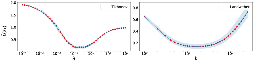
Figure 1: Empirical risk trajectories of the Tikhonov and Landweber regularization methods. The solid lines represent the mean value, while the shaded regions represent the $5^{\rm th}$-percentiles and $95^{\rm th}$-percentiles over 30 trials. The $x$-axis is shown in logarithmic scale.

6.1.1 Illustration of the data-driven parameter choice

We start considering the problem described in Section 6.1 with noise level $\tau^{2}=0.125$ and source condition $s=3$. Starting from the training set $\{(y_{i},x_{i})\}_{i=1}^{100}$, for every $\lambda\in\Lambda$, we define the empirical risk for the Tikhonov regularized solution as

(49) $$\widehat{L}(X_{\lambda})=\frac{1}{100}\sum_{i=1}^{100}\|TX_{\lambda}(y_{i})-x_{i}\|^{2},$$

where $X_{\lambda}(y_{i})=(A^{*}A+\lambda I)^{-1}A^{*}y_{i}$ (see Section 3). The empirical risk for the Landweber method is defined analogously, where in this case $X_{\lambda}(y_{i})=(I-\gamma A^{*}A)^{\lfloor 1/\lambda\rfloor}A^{*}y_{i}$ with $\gamma=0.2$. For both Tikhonov regularization and Landweber iteration, we build a grid of regularization parameters $\Lambda=\{\lambda_{1},\ldots,\lambda_{N}\}$ as in Assumption 3, namely with $\lambda_{j}=\lambda_{1}Q^{j-1}$ for $j=1,\ldots,N$ and $Q=(\lambda_{N}/\lambda_{1})^{1/(N-1)}$. For Tikhonov we choose $N=50$, $\lambda_{1}=10^{-4}$ and $\lambda_{N}=10^{2}$, with a resulting $Q\approx 1.3257$. For Landweber, we choose $N=50$, $\lambda_{1}=1/250$, $\lambda_{50}=1$, with a resulting $Q\approx 1.1193$.

In Figure 1, the function $\lambda\in\Lambda\mapsto\widehat{L}(X_{\lambda})$ is plotted for Tikhonov regularization. For Landweber, we plot the function in terms of number of iterations $k$. According to Section 2, the parameter proposed by our approach is $\widehat{\lambda}$ (or $\widehat{k}=\lfloor 1/\widehat{\lambda}\rfloor$ in the case of Landweber), where $\widehat{\lambda}$ is a minimizer of the curves in Figure 1.

6.1.2 Illustration of Theorem 2

In this section we investigate the dependence from the noise level $\tau$ of the error of $X_{\lambda_{*}}$, see equation (17) in Theorem 2. For every fixed variance $\tau^{2}>0$ of $\varepsilon$, let $\lambda_{*}(\tau)$, or $k_{*}(\tau)$ in the case of Landweber, be a minimizer of the expected error,

(50) $$\lambda_{*}(\tau)\in\operatorname*{arg\,min}_{\lambda\in(0,+\infty)}L(X_{\lambda}),$$

which we approximate through the corresponding empirical error $\widehat{L}(X_{\lambda})$, given by (49), with $n=10^{3}$ training points (recall that $L(X_{\lambda_{*}(\tau)})$, with $\lambda_{*}(\tau)$ defined as above, is a lower bound for the left hand side in equation (17)). As stated in Theorem 2, $L(X_{\lambda_{*}(\tau)})$ goes to zero when $\tau$ vanishes. The parameter $\alpha$ in Assumption 6 plays an important role in the bound, since $L(X_{\lambda_{*}(\tau)})\lesssim\tau^{\frac{4\alpha}{2\alpha+1}}$. In particular, we expect $L(X_{\lambda_{*}(\tau)})$ to go to $0$ faster when $\alpha$ increases. For Tikhonov, $\alpha=\min\{1,s\}$ (since $1$ is the qualification parameter for Tikhonov regularization). For Landweber, instead, $\alpha=s$. Therefore, in the experiments, we can vary $\alpha$ simply by choosing the value of the smoothness parameter $s$. The influence of $s$ on the decay rate of the reconstruction error is shown in Figure 2 for different values of $s$. To determine $\lambda_{*}(\tau)$ in the case of Tikhonov, we set a grid of $100$ equidistant points $\{\lambda_{i}\}_{i=1}^{100}$, $\lambda_{1}=10^{-5}$, $\lambda_{100}=0.5$, with a constant spacing of $0.005$ between consecutive points. We consider $50$ different values of the noise variance $\tau^{2}$, ranging from $10^{-5}$ to $0.1$. For the Landweber method, we opt for a set of $100$ points $\{\lambda_{i}\}_{i=1}^{100}$, with $\lambda_{1}=1/150$ and $\lambda_{100}=0.51$, and hence the optimal stopping time $k_{*}$ will be found in the range $k=1,\ldots,150$. We consider $50$ different values of the noise variance $\tau^{2}$ within the interval $[10^{-8},10^{-4}]$. Finally, for Tikhonov regularization, we choose the values $s=0.5,0.7\text{ and }0.9$, while for Landweber we choose $s=4,\ 5\text{ and }6$. The selected smoothness parameters allow us to gain a deeper insight into the behaviour of the expected error with respect to the deterministic rate obtained in Theorem 2. In Figure 2, we illustrate the quantity $L(X_{\lambda^{*}(\tau)})/\tau^{(4s)/(2s+1)}$, where it can be seen that all the curves, for every value of $s$, are bounded when $\tau$ goes to zero. We can also observe that the quantity of interest is not going to zero, therefore suggesting that the derived bounds are tight.

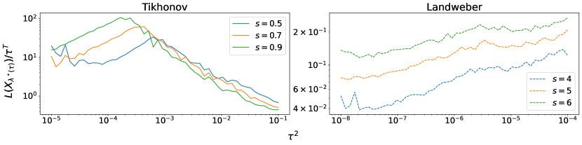
Figure 2: Behaviour of $L(f_{\lambda_{*}})$ with respect to the rate $\tau^{T}$, $T=(4s)/(2s+1)$, obtained in Theorem 2, for different smoothness parameters $s$ in the case of both Tikhonov and Landweber. Both axes are shown in logarithmic scale.

Finally, in order to explore Assumption 3, we will study the behaviour of the best empirical regularization parameters, $\widehat{\lambda}(\tau)$ and $\widehat{k}(\tau)$, with respect to the noise variance $\tau^{2}$ and the smoothness parameter $s$ for both Tikhonov and Landweber methods. Here, the empirical risk is computed with $100$ training points for smoothness parameters $s=0.5,\ 0.9$ in the case of Tikhonov and $s=2,\ 4$ in the case of Landweber. We fix $30$ different values of the noise variance, $\tau^{2}\in[10^{-4},0.1]$ with equal logarithmic spacing, and we consider the following grids: $\Lambda\subseteq[10^{-5},1]$ with $N=50$ and $Q\approx 1.2068$ in the case of Tikhonov regularization, and $\Lambda\subseteq[1/250,1]$ with $N=200$, and $Q\approx 1.0281$ for Landweber. Note that the seleted range for the noise variance in Figure 2 is different both for Tikhonov and Landweber. Indeed, the theoretical upper bound stated in Theorem 2 does not necessarily need to be observed, experimentally, in the exact same range for both cases.

Finally, it can be seen that the empirical parameters $\widehat{\lambda}(\tau)$ and $\widehat{k}(\tau)$ exhibit a similar behaviour to the a priori optimal ones [23]: in the case of Tikhonov regularization, it increases with the noise; i.e. $\lambda\sim\tau^{\rho}$ for some fixed $\rho>0$ (see [23, Chapter 5]), and in the case of Landweber, the number of iterations decreases with respect to the noise. For instance, the optimal stopping time in the discrepancy principle behaves as $k\sim(1/\tau)^{2/(2s+1)}$, $s$ being the smoothness parameter, see [23, Theorem 6.5]. In the latter case, it is clear that the smoothness of the solution has an effect in the regularization parameter, since for bigger values of $s$, the required optimal number of iterations is smaller. This behaviour can also be observed for our method in the corresponding image in Figure 3. The case of Tikhonov regularization is simpler to analyze. From (12), we observe that the regularization parameter should promote those solutions that are smoother or, in other words, for bigger values of the smoothness parameter $s$. This behaviour is actually confirmed by our experiments, as we observe in Figure 3.

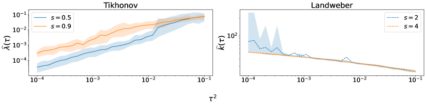
Figure 3: Value of $\widehat{\lambda}$, $\widehat{k}$ when varying the noise level for both Tikhonov Landweber. Both parameters have been selected over a training set of $100$ points, constructed with different smoothness parameters as shown in the plot. Solid lines represent the mean value, while the shaded regions represent the $5^{\rm th}$-percentiles and $95^{\rm th}$-percentiles over 30 trials. Both axis are shown in logarithmic scale.

6.1.3 Illustration of error bounds

In this section, we discuss some numerical experiments supporting the error bound stated in Corollary 1, both for Tikhonov and Landweber regularization methods. We use the grid $\Lambda$ introduced in Section 6.1.1, and we let $\lambda_{\Lambda}$ and $k_{\Lambda}$ be the parameters corresponding to the minimizers of the expected error –which we approximate with a minimizer of the empirical error with $n_{\max}=10^{5}$ points–. on the grid $\Lambda$ for Tikhonov and Landweber method, respectively. Moreover, we define the empirical error for every $n\in\{10,\ 20,...,\ 150\}$, where we sample fresh training points for every different value of $n$, and we denote by $\widehat{\lambda}(n)$ and $\widehat{k}(n)$ the parameters corresponding to the minimizers of the empirical error with $n$ points. We then define the quantity $\Delta(n):=L(X_{\widehat{\lambda}(n)})-L(X_{\lambda_{\Lambda}})$ (or $\Delta(n):=L(X_{\widehat{k}(n)})-L(X_{k_{\Lambda}})$ respectively). As stated in Corollary 1, the excess risk goes to zero, up to a certain additive constant, when $n$ goes to infinity, as confirmed by the plot in Figure 4.

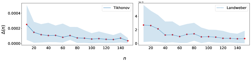
Figure 4: Excess risk behaviour with respect to the number of training points for noise level $\tau^{2}=0.2$. In the $y$-axis we plot the quantity $\Delta(n)$, showing that it goes to zero when $n$ increases. The solid lines represent the mean value, while the shaded regions represent the $5^{\rm th}$-percentiles and $95^{\rm th}$-percentiles over 30 trials.

6.1.4 Comparison with the quasi-optimality criterion

In this section we compare our data-driven approach to the quasi-optimality criterion [45]. The latter is one of the most common and simple-to-implement heuristic parameter selection methods and does not require the noise level to be computed. Theoretical guarantees on its performance are available in the stochastic inverse problem setting [6]. First, note that the computational cost of the two methods can be very different. The quasi-optimality criterion performs instance-wise as all the usual parameter selection methods; i.e. given a set of test data $\{(y_{i},x_{i})\}_{i=1}^{n_{\mathrm{test}}}$, $n_{\mathrm{test}}\in\mathbb{N}$, and a regularization method $X_{\lambda}$, it outputs the best regularization parameter $\widehat{\lambda}_{i}$ for each $y_{i}$, $i=1,...,n_{\mathrm{test}}$. This could lead to high computational costs when the number of test points is big. Indeed, the method needs to be run as many times as the number of points, and for each test point the computation of the whole regularization path is required (see below). On the contrary, our algorithm requires to have access to a training set, but then, on test problems, the learned parameter $\widehat{\lambda}$ will be the same for every $i=1,...,n_{\mathrm{test}}$, and only one regularized problem needs to be solved. In the following we compare the two approaches in terms of average performance on the test problems for Tikhonov and Landweber methods. For Tikhonov regularization, we fix a grid of regularization parameters $\Lambda\subseteq[10^{-5},10]$, with $N=50$, $Q\approx 1.3257$ and we denote $X_{i,{\lambda_{j}}}$ the solution of the regularized problem for the parameter $\lambda_{j}$ and datum $y_{i}$, $i\in\{1,\ldots,n_{\mathrm{test}}\}$. We fix $n_{\mathrm{test}}=100$. For each $(y_{i},x_{i})$ in the test set, we select the parameter with the quasi-optimality criterion, namely we set $\lambda^{\text{qo}}_{i}=\lambda_{j_{*}(i)}$, where $j_{*}(i)$ is defined as

$$j_{*}(i)\in\operatorname*{arg\,min}_{j\in{0,\ldots,50}}\|X_{i,\lambda_{j}}-X_{i,\lambda_{j+1}}\|.$$

Our method instead provides a unique $\widehat{\lambda}_{\Lambda}$, depending on the training set. For this experiment, we fix a training set of $10^{5}$ points. We then compare the average test error corresponding to the two methods, where, for the quasi-optimality criterion we consider

$$L^{\text{qo}}=\frac{1}{100}\sum_{i=1}^{100}\|X_{i,\lambda^{\text{qo}}_{i}}-x_{i}\|^{2}.$$

For Landweber iteration, we follow the implementation of the quasi-optimality criterion proposed in [4], and we define $\lambda^{\text{qo}}_{i}=\lambda_{j_{*}}$, where $j_{*}(i)$ is defined as

$$j_{*}(i)\in\operatorname*{arg\,min}_{j\in\{1/500,\ldots,1\}}\|X_{i,2\lfloor 1/\lambda_{j+1}\rfloor}-X_{i,\lfloor 1/\lambda_{j+1}\rfloor}\|,$$

and we compare the average test error as for the Tikhonov method.

We denote the test error corresponding to our method $L^{\text{learn}}$ (for both Tikhonov and Landweber) and we compute the quantity $L^{\text{learn}}-L^{\text{qo}}$ for $30$ different realizations of the training set. We show in Tables 1 and 2 the mean value and standard deviation of the proposed experiment for both Tikhonov and Landweber with source condition $s=3$. As the tables suggest, the data-driven selection method performs differently than the quasi-optimality criterion for both the Tikhonov and Landweber regularization. First, observe that, in the case of Tikhonov regularization, the difference between the two studied methods is small when the noise variance is small. Instead, when such noise variance increases, the learned regularization parameter performs better. In the case of Landweber, instead, it can be seen in 2 that the learned regularization parameter performs considerably better for all of the proposed quantities of the noise variance, maintaining at the same time considerably low values for the standard deviation.

$L^{\text{learn}}-L^{\text{qo}}$, Tikhonov
noise var.	$\tau^{2}=10^{-4}$	$\tau^{2}=10^{-3}$	$\tau^{2}=10^{-2}$	$\tau^{2}=1$
mean	$-1.32\times 10^{-7}$	$-5.46\times 10^{-5}$	$-1.08\times 10^{-4}$	$-0.2964$
std	$2.64\times 10^{-23}$	$1.20\times 10^{-6}$	$2.40\times 10^{-5}$	$4.16\times 10^{-2}$

Table 1: Mean value and standard deviation of the error difference between our method and the quasi-optimality criterion. Above, we compare methods in the case of Tikhonov regularization for different values of the noise variance.

$L_{\text{learn}}-L^{\text{qo}}$, Landweber
noise var.	$\tau^{2}=10^{-4}$	$\tau^{2}=10^{-3}$	$\tau^{2}=10^{-2}$	$\tau^{2}=1$
mean	$-0.0605$	$-0.7880$	$-0.9999$	$-0.2937$
std	$6.93\times 10^{-18}$	$2.22\times 10^{-16}$	$1.11\times 10^{-16}$	$0$

Table 2: Mean value and standard deviation of the error difference between our method and the quasi-optimality criterion. Above, we compare methods for the Landweber iteration with different values of the noise variance.

6.2 Sparsity inducing regularizers

In this section, we explore the theoretical results in Section 5.1 for three different examples: denoising and deblurring of a sparse signal, and Total Variation regularization for image denoising. We start with the simplest case: denoising of a sparse signal.

6.2.1 Denoising of a sparse signal

Let $x^{*}\in\mathbb{R}^{d}$ be an $s$-sparse signal; i.e., a signal with $s$ nonzero entries, and consider the white noise model $\varepsilon\sim N(0,\tau^{2}\mathrm{Id})$, with variance $\tau^{2}>0$. We consider the denoising problem

(51) $$y=x^{*}+\varepsilon,$$

where $x^{*}$ is such that $\|x^{*}\|_{2}\leq 1$ as required by Assumption 12. The most classical approach to recover $x^{*}$ having access only to $y$ is to solve the Lasso problem [43],

(52) $$\min_{x\in\mathbb{R}^{d}}\frac{1}{2}\|x-y\|^{2}_{2}+\lambda\|x\|_{1}.$$

where the $\ell^{1}$ norm promotes sparsity [17]. In this case, it is easy to show that the solution admits a closed-form expression, that is

$$X_{\lambda}=\mathcal{S}_{\lambda}(y),\quad\lambda\in(0,+\infty),$$

where $\mathcal{S}_{\lambda}$ denotes the so-called soft-thresholding operator, introduced in [22], is defined componetwise as

$$(\mathcal{S}\lambda(y))_{i}:=\begin{cases}\quad 0,&\text{ if }|y_{i}|\leq\lambda,\\ y_{i}-\lambda\mathrm{sign}(y_{i}),&\text{ if }|y_{i}|>\lambda,\end{cases}$$

for every $i\leq d$. In this section, we will illustrate, from a numerical point of view, Corollary 7 for this setting. We therefore aim at showing that the excess risk for this problem goes to zero as $n$ goes to infinity, up to a certain additive constant. To do so, we first fix $d=1024$, $s=16$, $\tau^{2}=0.1$. Then, we fix a grid of regularization parameters of $N=50$ points $\Lambda=\{\lambda_{1},...,\lambda_{50}\}\subseteq[10^{-4},10]$, with $Q\approx 1.2648$ and, for every $n\in\{10,...,150\}$ we define $\widehat{\lambda}(n)$ as a minimizer of the empirical risk,

$$\widehat{\lambda}(n)\in\operatorname*{arg\,min}_{\lambda\in\Lambda}\displaystyle\frac{1}{n}\sum_{i=1}^{n}D_{\|\cdot\|_{1}}(x_{i},\mathcal{S}_{\lambda}(y_{i})).$$

where, for every $n$, we consider an independent set of training points $\{(y_{i},x_{i})\}_{i=1}^{n}$, generated according to (51). Finally, we let $\lambda_{\Lambda}$ be the minimizer of the expected error (43), which we approximate with a minimizer of the empirical error with $n_{\mathrm{max}}=10^{5}$ training points. We let $\Delta(n)=L(\mathcal{S}_{\widehat{\lambda}(n)}(y))-L(\mathcal{S}_{\lambda_{\Lambda}}(y))$ denote the excess risk. In Figure 5, we plot the quantity $\Delta(n)$ for every $n\in\{10,...,150\}$, showing that, empirically, the excess risk goes to $0$, up to a certain additive constant, when the number of points goes to infinity.

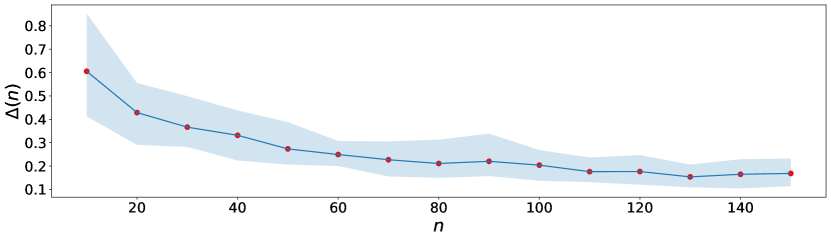
Figure 5: Excess risk behaviour of the signal denoising problem with respect to the number of training points. In the $y$-axis we plot the quantity $\Delta(n)$, showing that it goes to zero when $n$ increases. The solid lines represent the mean value, while the shaded regions represent the $5^{\rm th}$-percentiles and $95^{\rm th}$-percentiles over 30 trials.

6.2.2 Deblurring of a sparse signal

In this section, we consider the deblurring of a sparse signal. Our aim is to recover a sparse signal $x^{*}\in\mathbb{R}^{256}$ that has been corrupted via a convolution operator $A$ and additive noise:

(53) $$y=Ax^{*}+\varepsilon,$$

where $x^{*}$ is an $8$-sparse signal such that $\|x^{*}\|_{2}\leq 1$, as required by Assumption 12, and $\varepsilon\sim N(0,\tau^{2}\mathrm{Id})$ as pointed in Assumption 4. Moreover, the forward mapping $A$ is a linear convolution operator

$$x\in\mathbb{R}^{256}\mapsto Ax=h\ast x\in\mathbb{R}^{256},$$

with $h$ the second derivative of a Gaussian. More precisely, let $\phi(x)=e^{-x^{2}/(2\pi^{2})}$, then $h=\phi^{\prime\prime}-\mu(\phi^{\prime\prime})$, being $\mu(\phi^{\prime\prime})$ the expectation of $\phi^{\prime\prime}$. In order to recover $x^{*}$, we solve the following variational problem

$$\min_{x}\frac{1}{2}\|Ax-y\|^{2}_{\mathcal{Y}}+\lambda\|x\|_{1},$$

running the FISTA algorithm with constant stepsize [9] until convergence; i.e. until the difference between iterates is smaller than $10^{-6}$.

Next, we aim at illustrating Corollary 7; i.e., showing the error behaviour of the learned regularization parameter when $n$ goes to infinity. For this example, we fix $\tau^{2}=0.01$ and the regularization method $X_{\lambda}$ to be the output of running the FISTA algorithm as explained above. Then, we fix the grid of admissible regularization parameters to be $\Lambda\subseteq[10^{-2},1]$ with $N=50$ and $Q\approx 1.0985$. The ERM writes as

$$\widehat{\lambda}(n)\in\operatorname*{arg\,min}_{\lambda\in\Lambda}\displaystyle\frac{1}{n}\sum_{i=1}^{n}D_{\|\cdot\|_{1}}(x_{i},X_{\lambda}(y_{i})).$$

where, for every $n\in\{10,...,150\}$, we consider independent sets of training points $\{(y_{i},x_{i})\}_{i=1}^{n}$, that have been generated according to (53). Finally, let $\lambda_{\Lambda}$ be the minimizer of the expected error (43) –which we approximate through the empirical error with $n_{\text{max}}=10^{5}$ training points–, and define $\Delta(n)=L(X_{\widehat{\lambda}(n)})-L(X_{\lambda_{\Lambda}})$ to be the excess risk. According to Corollary 7, it should go to zero as $n$ goes to infinity, up to a certain additive constant. We show in Figure 6 the quantity $\Delta(n)$ for every $n\in\{10,...,150\}$.

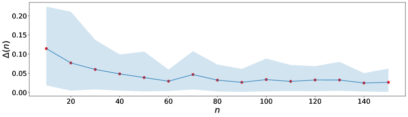
Figure 6: Excess risk behaviour of the signal deblurring problem with respect to the number of training points. In the $y$-axis we plot the quantity $\Delta(n)$, showing that it decreases to zero with $n$ going to infinity. The solid lines represent the mean value, while the shaded regions represent the $5^{\rm th}$-percentiles and $95^{\rm th}$-percentiles over 30 trials.

Finally, we show one example of a reconstructed signal using our regularization parameter choice. In order to learn the parameter $\widehat{\lambda}$, we first construct a training set of $n_{\mathrm{train}}=100$ clean/corrupted signals with the same distribution as the test element that we want to reconstruct, with noie variance $\tau^{2}=2.5\times 10^{-3}$. Then, the regularization parameter will be the minimizer of the empirical risk (44) with respect to the fixed training set. We show in the third row of Figure 7, the resulting regularized solution with the learned regularization parameter.

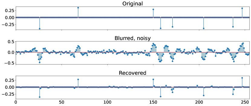
Figure 7: Deblurring of a sparse noisy, blurred signal with learned regularization parameter. In the first row, we show the original signal; in the second, its blurred and noisy version; and in the third row, the regularized solution with learned regularization parameter.

6.2.3 Total Variation for image denoising

In this section, we use our data-driven algorithm for choosing the regularization parameter of a Total Variation regularizer [14, 39]. To do so, we focus on the image denoising problem

(54) $$y=x^{*}+\varepsilon.$$

where $x$, $y\in\mathbb{R}^{d\times d}$, $d\in\mathbb{N}$. A classical approach to solve (54) is to rely on the following variational approach [41]

(55) $$\min_{x}\frac{1}{2}\|x-y\|_{2}^{2}+\lambda\mathrm{TV}(x),$$

where

$$\mathrm{TV}(x)=\|Dx\|_{1},$$

and $Dx=(D_{1}x,D_{2}x)\in\mathbb{R}^{2d(d-1)}$ is the discrete derivative, defined as in [13]. Then, we propose as regularization method $X_{\lambda}$ a solution of problem (55). Since (55) does not have a closed-form solution, we compute it by running the FISTA algorithm on the dual problem of (55), until convergence (i.e. until the difference between iterates is smaller than $10^{-8}$). First, we show the error behaviour of the learned regularization parameter plot for this example, illustrating Corollary 7.

We consider the MNIST dataset of $28\times 28$ images of digits from $0$ to $9$, and corrupt them as follows: every clean image $x^{*}\in\mathbb{R}^{28\times 28}$, will be corrupted as in (54) with Gaussian noise $\varepsilon\sim N(0,\tau^{2}\mathrm{Id})$. We fix the noise variance to be $\tau^{2}=0.01$ for this section. Then, we fix a grid of $N=50$ points $\Lambda=\{\lambda_{1},...,\lambda_{50}\}\subseteq[10^{-4},10^{-1}]$, with $Q\approx 1.1514$. For every $n\in\{10,...,100\}$, we let $\widehat{\lambda}(n)$ be a minimizer of the empirical risk,

$$\widehat{\lambda}(n)\in\operatorname*{arg\,min}_{\lambda\in\Lambda}\displaystyle\frac{1}{n}\sum_{i=1}^{n}D_{\mathrm{TV}}(x_{i},X_{\lambda}(y_{i})).$$

where, for every $n$, we consider an independent training set of points $\{(y_{i},x_{i})\}_{i=1}^{n}$ randomly selected from a set of $3\times 10^{3}$ images. The best regularization parameter $\lambda_{\Lambda}$ is the minimizer of the expected error (43), which we approximate with $n_{\mathrm{max}}=7\times 10^{3}$ training points constructed as in (54). With this, we define the excess risk as $\Delta(n)=L(X_{\widehat{\lambda}(n)})-L(X_{\lambda_{\Lambda}})$. As shown in Figure 8, the quantity $\Delta(n)$ goes to zero when $n$ goes to infinity, up to a certain constant, as indicated in Corollary 7.

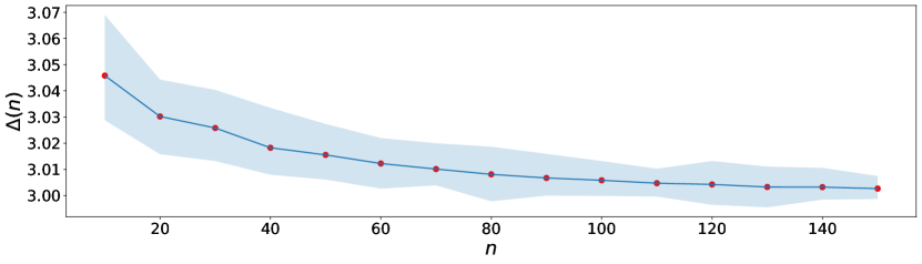
Figure 8: Excess risk behaviour of the Total Variation denoising problem with respect to the number of training points. In the $y$-axis we plot the quantity $\Delta(n)$, showing that it goes to zero when $n$ increases. The solid lines represent the mean value, while the shaded regions represent the $5^{\rm th}$-percentiles and $95^{\rm th}$-percentiles over 30 trials.

Finally, as an illustrative example, we explore the performance of the studied parameter selection method on test images from the MNIST dataset. We compute four different data-driven regularization parameters for four different training sets, each of $100$ training points, and check the reconstruction results of the TV regularized solution for two different digits in the test set. The results are shown in Figure 9. We observe that the recovery results on single test images may vary depending on the set of points that was used for training. This is expected, since our parameter selection method has been designed in order to perform effectively on average.

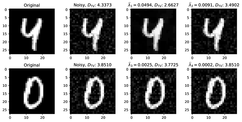
Figure 9: Total Variation denoising algorithm for two digit in the test set. From left to right, in every row, we plot the original image, its noisy version, and the recovery obtained with different regularization parameters. We also include, accordingly, the Bregman distance with respect to the original image and the value of the regularization parameter that has been used for such recovery.

7 Conclusions

In this paper, we studied the problem of learning the regularization parameter for regularization methods in inverse problems. Such topic has gained atention in the past years due to its promising results in many applications [32, 33, 42], since it does not require to have any prior knowledge neither on the noise level nor on the ground truth. By applying statistical learning techniques [16, 46], we were able to characterize the error performance of this method following an empirical risk minimization approach. Various numerical experiments have been included in order to validate and illustrate the theoretical findings.

Our analysis studies a wide variety of regularization methods, including spectral regularization methods (Tikhonov regularization, Landweber iteration, the $\nu$-method), non-linear Tikhonov regularization [23] and general convex regularizers such as sparsity inducing norms [3] and Total Variation regularization [39].

An interesting research direction is the analysis of state-of-the-art approaches involving deep learning methods. We believe that our results are a step forward towards understanding the underlying theoretical principles that govern the iteraction between classical regularization techniques and data-driven/learning approaches. This comprehension is crucial as it could substantially enhance our confidence in using these hybrid models, validating their combined use.

8 Acknowledgements

This project has been supported by the TraDE-OPT project, which received funding from the European Union’s Horizon 2020 research and innovation program under the Marie Skłodowska-Curie grant agreement No 861137. L. R. acknowledges the financial support of the European Research Council (grant SLING 819789), the AFOSR projects FA9550-18-1-7009 (European Office of Aerospace Research and Development), the EU H2020-MSCA-RISE project NoMADS - DLV-777826, and the Center for Brains, Minds and Machines (CBMM), funded by NSF STC award CCF-1231216. S. V. and L. R. acknowledge the support of the AFOSR project FA8655-22-1-7034. The research by E.D.V., S. V. and C. M. has been supported by the MIUR Excellence Department Project awarded to Dipartimento di Matematica, Università di Genova, CUP D33C23001110001. E.D.V., S. V. and C. M. are members of the Gruppo Nazionale per l’Analisi Matematica, la Probabilità e le loro Applicazioni (GNAMPA) of the Istituto Nazionale di Alta Matematica (INdAM). This work represents only the view of the authors. The European Commission and the other organizations are not responsible for any use that may be made of the information it contains.

References

- [1] G. S. Alberti, E. De Vito, M. Lassas, L. Ratti, and M. Santacesaria, Learning the optimal tikhonov regularizer for inverse problems, in Advances in Neural Information Processing Systems, vol. 34, Curran Associates, Inc., 2021, pp. 25205–25216, https://proceedings.neurips.cc/paper_files/paper/2021/file/d3e6cd9f66f2c1d3840ade4161cf7406-Paper.pdf.
- [2] S. Arridge, P. Maass, O. Öktem, and C.-B. Schönlieb, Solving inverse problems using data-driven models, Acta Numerica, 28 (2019), pp. 1–174, https://doi.org/10.1017/S0962492919000059.
- [3] F. Bach, R. Jenatton, J. Mairal, G. Obozinski, et al., Optimization with sparsity-inducing penalties, Foundations and Trends® in Machine Learning, 4 (2012), pp. 1–106.
- [4] F. Bauer and M. A. Lukas, Comparing parameter choice methods for regularization of ill-posed problems, Mathematics and Computers in Simulation, 81 (2011), pp. 1795–1841, https://doi.org/https://doi.org/10.1016/j.matcom.2011.01.016.
- [5] F. Bauer, S. Pereverzev, and L. Rosasco, On regularization algorithms in learning theory, J. Complexity, 23 (2007), pp. 52–72.
- [6] F. Bauer and M. Reiß, Regularization independent of the noise level: an analysis of quasi-optimality, Inverse Problems, 24 (2008), p. 055009, https://doi.org/10.1088/0266-5611/24/5/055009.
- [7] H. H. Bauschke, J. M. Borwein, and P. L. Combettes, Essential smoothness, essential strict convexity, and legendre functions in banach spaces, Communications in Contemporary Mathematics, 03 (2001), pp. 615–647, https://doi.org/10.1142/S0219199701000524.
- [8] H. H. Bauschke and P. L. Combettes, Convex analysis and monotone operator theory in Hilbert spaces, CMS Books in Mathematics/Ouvrages de Mathématiques de la SMC, Springer, New York, 2011, https://doi.org/10.1007/978-1-4419-9467-7.
- [9] A. Beck and M. Teboulle, A fast iterative shrinkage-thresholding algorithm for linear inverse problems, SIAM Journal on Imaging Sciences, 2 (2009), pp. 183–202, https://doi.org/10.1137/080716542.
- [10] M. Benning and M. Burger, Modern regularization methods for inverse problems, Acta Numerica, 27 (2018), pp. 1–111, https://doi.org/10.1017/S0962492918000016.
- [11] M. Burger, E. Resmerita, and L. He, Error estimation for Bregman iterations and inverse scale space methods in image restoration, Computing, 81 (2007), pp. 109–135, https://doi.org/10.1007/s00607-007-0245-z.
- [12] A. Caponnetto and Y. Yao, Cross-validation based adaptation for regularization operators in learning theory, Analysis and Applications, 08 (2010), pp. 161–183, https://doi.org/10.1142/S0219530510001564.
- [13] A. Chambolle, An algorithm for total variation minimization and applications, Journal of Mathematical Imaging and Vision, 20 (2004), pp. 89–97, https://doi.org/10.1023/B:JMIV.0000011325.36760.1e.
- [14] A. Chambolle and P.-L. Lions, Image recovery via total variation minimization and related problems, Numerische Mathematik, 76 (1997), pp. 167–188.
- [15] C. Clason, Regularization of inverse problems, 2021, https://arxiv.org/abs/2001.00617.
- [16] F. Cucker and S. Smale, On the mathematical foundations of learning, Bull. Amer. Math. Soc. (N.S.), 39 (2002), pp. 1–49, https://doi.org/10.1090/S0273-0979-01-00923-5.
- [17] I. Daubechies, M. Defrise, and C. De Mol, An iterative thresholding algorithm for linear inverse problems with a sparsity constraint, Communications on Pure and Applied Mathematics, 57 (2004), pp. 1413–1457, https://doi.org/https://doi.org/10.1002/cpa.20042.
- [18] E. De Vito, M. Fornasier, and V. Naumova, A machine learning approach to optimal tikhonov regularization I: Affine manifolds, Analysis and Applications, 20 (2022), pp. 353–400, https://doi.org/10.1142/S0219530520500220.
- [19] C.-A. Deledalle, S. Vaiter, J. Fadili, and G. Peyré, Stein unbiased gradient estimator of the risk (sugar) for multiple parameter selection, SIAM Journal on Imaging Sciences, 7 (2014), pp. 2448–2487, https://doi.org/10.1137/140968045.
- [20] L. Deng, The mnist database of handwritten digit images for machine learning research, IEEE Signal Processing Magazine, 29 (2012), pp. 141–142, https://doi.org/10.1109/MSP.2012.2211477.
- [21] L. Devroye, L. Györfi, and G. Lugosi, A probabilistic theory of pattern recognition, vol. 31 of Applications of Mathematics (New York), Springer-Verlag, New York, 1996, https://doi.org/10.1007/978-1-4612-0711-5.
- [22] D. L. Donoho and I. M. Johnstone, Adapting to unknown smoothness via wavelet shrinkage, Journal of the American Statistical Association, 90 (1995), pp. 1200–1224, https://doi.org/10.1080/01621459.1995.10476626.
- [23] H. W. Engl, M. Hanke, and A. Neubauer, Regularization of inverse problems, vol. 375 of Mathematics and its Applications, Kluwer Academic Publishers Group, Dordrecht, 1996, https://doi.org/10.1007/978-3-540-70529-1_52.
- [24] L. Franceschi, P. Frasconi, S. Salzo, R. Grazzi, and M. Pontil, Bilevel programming for hyperparameter optimization and meta-learning, in Proceedings of the 35th International Conference on Machine Learning, vol. 80, PMLR, 2018, pp. 1568–1577.
- [25] G. H. Golub and U. von Matt, Generalized cross-validation for large-scale problems, Journal of Computational and Graphical Statistics, 6 (1997), pp. 1–34, https://doi.org/10.2307/1390722.
- [26] M. Grasmair, M. Haltmeier, and O. Scherzer, Sparse regularization with lq penalty term, Inverse Problems, 24 (2008), p. 055020, https://doi.org/10.1088/0266-5611/24/5/055020.
- [27] L. Györfi, M. Kohler, A. Krzyżak, and H. Walk, A distribution-free theory of nonparametric regression, Springer Series in Statistics, Springer-Verlag, New York, 2002, https://doi.org/10.1007/b97848.
- [28] P. C. Hansen, Analysis of discrete ill-posed problems by means of the l-curve, SIAM Review, 34 (1992), pp. 561–580, https://doi.org/10.1137/1034115.
- [29] T. Hastie, R. Tibshirani, and M. Wainwright, Statistical Learning with Sparsity: The Lasso and Generalizations, Chapman & Hall/CRC, 2015.
- [30] C. J. Himmelberg, Measurable relations, Fundamenta Mathematicae, 87 (1975), pp. 53–72.
- [31] Z. Kereta and V. Naumova, On an unsupervised method for parameter selection for the elastic net, Mathematics in Engineering, 4 (2022), pp. 1–36, https://doi.org/10.3934/mine.2022053.
- [32] E. Kobler, A. Effland, K. Kunisch, and T. Pock, Total deep variation for linear inverse problems, in 2020 IEEE/CVF Conference on Computer Vision and Pattern Recognition (CVPR), 2020, pp. 7546–7555, https://doi.org/10.1109/CVPR42600.2020.00757.
- [33] K. Kunisch and T. Pock, A bilevel optimization approach for parameter learning in variational models, SIAM Journal on Imaging Sciences, 6 (2013), pp. 938–983, https://doi.org/10.1137/120882706.
- [34] N. Meinshausen and P. Bühlmann, High-dimensional graphs and variable selection with the Lasso, The Annals of Statistics, 34 (2006), pp. 1436–1462, https://doi.org/10.1214/009053606000000281.
- [35] V. A. Morozov, On the solution of functional equations by the method of regularization, in Doklady Akademii Nauk, vol. 167, Russian Academy of Sciences, 1966, pp. 510–512.
- [36] S. Mosci, L. Rosasco, M. Santoro, A. Verri, and S. Villa, Solving structured sparsity regularization with proximal methods, in Machine Learning and Knowledge Discovery in Databases. ECML PKDD 2010. Lecture Notes in Computer Science, 2010, pp. 418–433.
- [37] A. Neubauer, On nesterov acceleration for landweber iteration of linear ill-posed problems, Journal of Inverse and Ill-posed Problems, 25 (2017), pp. 381–390, https://doi.org/doi:10.1515/jiip-2016-0060.
- [38] G. Peyré, The numerical tours of signal processing, Computing in Science & Engineering, 13 (2011), pp. 94–97, https://doi.org/10.1109/MCSE.2011.71.
- [39] L. I. Rudin, S. Osher, and E. Fatemi, Nonlinear total variation based noise removal algorithms, Physica D: Nonlinear Phenomena, 60 (1992), pp. 259–268, https://doi.org/https://doi.org/10.1016/0167-2789(92)90242-F.
- [40] S. Salzo and S. Villa, Proximal Gradient Methods for Machine Learning and Imaging, Springer International Publishing, 2021, pp. 149–244, https://doi.org/10.1007/978-3-030-86664-8_4.
- [41] O. Scherzer, M. Grasmair, H. Grossauer, M. Haltmeier, and F. Lenzen, Variational methods in imaging, vol. 167, Springer, 2009.
- [42] F. Sherry, M. Benning, J. Reyes, M. Graves, G. Maierhofer, G. Williams, C.-B. Schönlieb, and M. Ehrhardt, Learning the sampling pattern for MRI, IEEE Transactions on Medical Imaging, 39 (2020), pp. 4310–4321, https://doi.org/10.1109/TMI.2020.3017353.
- [43] R. Tibshirani, Regression shrinkage and selection via the lasso, Journal of the Royal Statistical Society. Series B (Methodological), 58 (1996), pp. 267–288, http://www.jstor.org/stable/2346178.
- [44] A. N. Tikhonov and V. Y. Arsenin, Solutions of ill-posed problems, Scripta Series in Mathematics, V. H. Winston & Sons, Washington, D.C.; John Wiley & Sons, New York-Toronto, Ont.-London, 1977.
- [45] A. N. Tikhonov, V. B. Glasko, and Y. A. Kriksin, On the question of quasi-optimal choice of a regularized approximation, in Doklady Akademii Nauk, vol. 248, Russian Academy of Sciences, 1979, pp. 531–535.
- [46] V. Vapnik, The nature of statistical learning theory, Springer science & business media, 1999.
- [47] G. Wahba, Practical approximate solutions to linear operator equations when the data are noisy, SIAM Journal on Numerical Analysis, 14 (1977), pp. 651–667, https://doi.org/10.1137/0714044.
- [48] D. Williams, Probability with Martingales, Cambridge University Press, 1991, https://doi.org/10.1017/CBO9780511813658.