New Developments in the Numerical Conformal Bootstrap

Abstract

The numerical conformal bootstrap has become in the last 15 years an indispensable tool for studying strongly coupled CFTs in various dimensions. Here we review the main developments in the field in the last 5 years, since the appearance of the previous comprehensive review Poland:2018epd . We describe developments in the software (SDPB 2.0, scalar_blocks, blocks_3d, autoboot, hyperion, simpleboot), and on the algorithmic side (Delauney triangulation, cutting surface, tiptop, navigator function, skydive). We also describe the main physics applications which were obtained using the new technology.

CALT-TH 2023-046

1 Introduction

Since its inception 15 years ago Rattazzi:2008pe , the numerical conformal bootstrap has become an indispensable tool for studying strongly coupled CFTs in various dimensions. The 2018 review Poland:2018epd covered thoroughly the first 10 years of these developments. Since then, software and algorithmic advances led to marked increase in the sophistication of performed computations, and to a number of spectacular breakthroughs. Here we will review these recent exciting developments. Our review is complementary to another recent review Poland:2022qrs . We cover a larger number of topics and go more in-depth in the description of the algorithms and of the results.

We start by describing the developments in the software allowing to perform the convex optimization, compute conformal blocks, and organize the computations (Section 2). We then present a few physics results which were achieved only thanks to the software developments (Section 3). In the next several section we describe the main algorithmic developments (Delaunay triangulation, surface cutting, tiptop, the navigator function, and skydive), together with the physics results achieved thanks to them. We then conclude with prospects for future developments.

2 Software developments

The most important software development was the release of SDPB 2.0 Landry:2019qug , a new version of the main bootstrap code SDPB Simmons-Duffin:2015qma . SDPB implements a primal-dual interior-point method for solving semidefinite programs (SDPs), taking advantage of sparsity patterns in matrices that arise in bootstrap problems, and using arbitrary-precision arithmetic to deal with numerical instabilities when inverting poorly-conditioned matrices.

The new version has improved the parallelization support. SDPB 1.0 could only run on a single cluster node, using all cores of that node. SDPB 2.0 can run on multiple cluster nodes with hundreds of cores. The speedup is proportional to the number of available cores. In addition, every core needs only a part of the input data, decreasing the amount of needed memory per node. Provided that one has access to a big cluster, SDPB 2.0 can perform large computations which with SDPB 1.0 would take too long to complete, or would not even fit on a single cluster node due to memory limitations.

2.1 Conformal blocks

To setup a bootstrap computation, one needs to precompute $z,\bar{z}$ derivatives of conformal blocks. Up to a prefactor, they can be approximated by polynomials of the exchanged primary dimension. These polynomials are then processed by a framework software (Section 2.2) and passed to SDPB.

The simplest blocks are for the scalar external operators (“scalar blocks”). Many bootstrap studies computed them used an algorithm from ElShowk:2012ht ; El-Showk:2014dwa , implemented in Mathematica. This was limited by the number of Mathematica licenses available on the cluster. Recently, the algorithm was re-implemented as a fast open-source C++ program scalar_blocks scalarblocks . It computes scalar blocks in any spacetime dimension $d$, both integer and non-integer.

Spinning external operators (such as fermions, conserved currents, and the stress tensor) are playing an increasingly important role in the bootstrap. Their conformal blocks are more complicated than scalar blocks. Previously, spinning operator studies relied on Mathematica codes to compute the blocks. Recently, a C++ program blocks_3d Erramilli:2019njx ; Erramilli:2020rlr was released, which computes $d=3$ conformal blocks for external and exchanged operators of arbitrary spins.

2.2 Frameworks

A bootstrap framework is a software suite which, given problem specifications, generates CFT bootstrap equations, computes $z,\bar{z}$ derivatives of the crossing equation terms from the conformal block derivatives, generates SDPB input files, launches SDPB computations and supervises them. Several frameworks have been developed, the most powerful being hyperion hyperion in Haskell, and simpleboot simpleboot in Mathematica, These frameworks also have support for scalar_blocks, blocks_3d, SDPB 2.0, as well as the algorithms discussed in later sections of this review (Delauney triangulation, surface sutting, the navigator function and the skydive). Other frameworks include juliBootS Paulos:2014vya in Julia, and PyCFTBoot Behan:2016dtz , cboot cboot in Python.

For CFTs with global symmetry, the bootstrap equations involves the crossing kernels (6-j symbols) of the group. For finite groups and Lie groups with a small number of generators, autoboot Go:2019lke ; Go:2020ahx is a package designed to automate the derivation of the crossing kernel and produce bootstrap equations for scalar correlators. The package uses cboot as a framework software to launch SDPB. The framework simpleboot can also work with the bootstrap equations produced by autoboot.

3 Pushing the old method

In years 2015-2020 numerical bootstrap studies were mostly performed using the following approach Kos:2014bka ; Simmons-Duffin:2015qma . The bootstrap equations are truncated by taking the derivatives at the crossing symmetric point. Derivatives of the conformal block are approximated by polynomials, up to a positive prefactor. Together with certain assumptions on CFT data, the bootstrap equation is translated into an SDP problem. The SDP is solved in the “feasibility mode” to determine whether the assumptions are allowed or disallowed. Parameters of the theory space are scanned over using bisection or the Delaunay search (see section 4.1). With this method (referred to in this review as “the old method”), the number of parameters usually cannot be too large. However, many interesting results have been produced in the last few years using this method, especially thanks to the software developments described in section 2. In this section, we will review some of those results. Most computations in this section used SDPB 2.0 to solve SDPs, and would not have been possible with SDPB 1.0.

3.1 3D ${\cal N}=1$ supersymmetric Ising CFT

The Gross-Neveu-Yukawa model with one Majorana spinor is described by the following Lagrangian

$$\mathcal{L}=\frac{1}{2}(\partial_{\mu}\sigma)^{2}+m^{2}\sigma^{2}+\bar{\psi}\not{\partial}\psi+\frac{\lambda_{1}}{2}\sigma\bar{\psi}{\psi}+\frac{\lambda_{2}^{2}}{8}\sigma^{4},$$ (1)

where $\psi$ is a three-dimensional Majorana spinor. The Lagrangian is invariant under the time-reversal symmetry (T-parity) where $\sigma\rightarrow-\sigma$ and $\psi\rightarrow\gamma^{0}\psi$. In the UV, when $\lambda_{1}=\lambda_{2}$ and $m=0$, the model becomes $\mathcal{N}=1$ SUSY Wess-Zumino model with superpotential $\mathcal{W}=\lambda\Sigma^{3}$ and $\Sigma=\sigma+\bar{\theta}\psi+\frac{1}{2}\bar{\theta}\theta\epsilon$. For a particular value of the mass term $m^{2}$, the model flows in the IR to a fixed point referred to as the 3D ${\cal N}=1$ SUSY Ising CFT. The SUSY is explicitly broken for generic values $\lambda_{1}\neq\lambda_{2}$. However, the SUSY could emerge in the IR from a non-supersymmetric system by tuning a single macroscopic parameter, provided there is only one relevant singlet under T-parity Grover:2013rc . Ref. Grover:2013rc argued that this fixed point might be realized as a quantum critical point at the boundary of a $3+1$D topological superconductor.

The 3D ${\cal N}=1$ SUSY Ising CFT was first studied via bootstrap techniques using a single correlator of a scalar Bashkirov:2013vya or a fermion Iliesiu:2015qra (see Poland:2018epd for a review). Later, Refs. Rong:2018okz ; Atanasov:2018kqw extended the analysis to correlators involving $\sigma,\epsilon$. From a non-SUSY point of view, the bootstrap setup is same as the 3D Ising $\sigma,\epsilon$ setup of Kos:2014bka , where $\mathbb{Z}_{2}$ is realized by T-parity. Supersymmetry imposes additional constraints: $\Delta_{\epsilon}=\Delta_{\sigma}+1$, since $\sigma$ and $\epsilon$ are in the same supermultiplet, and the OPE coefficients $\lambda_{\sigma\sigma O}$, $\lambda_{\epsilon\epsilon O}$ are related to $\lambda_{\sigma\epsilon O^{\prime}}$, where $O$ and $O^{\prime}$ belong to the same supermultiplet. Ref. Rong:2018okz thoroughly worked out those constraints and injected them into the $\sigma,\epsilon$ setup. By demanding that, under T-parity, only one even scalar operator and two odd scalar operators are relevant, Ref. Rong:2018okz isolated the CFT as a small island in the theory space and produced precise critical exponents with rigorous error bars: $\eta_{\sigma}=0.168888({\bf 60})$ and $\omega=0.882({\bf 9})$. This provides strong evidence that the theory has superconformal symmetry and has only one relevant singlet under T-parity, confirming the possibility of emergent supersymmetry.

There are two follow up works Rong:2019qer ; Atanasov:2022bpi . As of 2023, the most precise conformal data for this CFT was obtained from Atanasov:2022bpi , using the same setup as Rong:2018okz but at a much higher $\Lambda=59$. The computation at such a high $\Lambda$ becomes practically feasible by utilizing scalar_blocks and SDPB 2.0. The result is summarized in Table 1.

CFT data	critical exponents
$\Delta_{\sigma}$=0.5844435(83)	$\begin{aligned} \eta_{\sigma}=\eta_{\psi}&=0.168887({\bf 17})\\ 1/\nu&=1.415557({\bf 8})\end{aligned}$
$\Delta_{\sigma^{\prime}}$=2.8869(25)	$\omega=0.8869({\bf 25})$

Table 1: Results of Atanasov:2022bpi for the scaling dimensions of $\Delta_{\sigma}$, $\Delta_{\sigma^{\prime}}$. Uncertainties in bold are rigorous.

The work Rong:2019qer studied more general $\mathcal{N}=1$ Wess-Zumino models with global symmetries, obtaining strong bounds on CFT data. However, no small bootstrap island has been identified. The bootstrapping of generic SUSY Wess-Zumino models remains a challenging task.

3.2 Bootstrapping critical gauge theories

An important class of CFTs are critical gauge theories, i.e. IR fixed point of abelian or non-abelian gauge fields coupled to matter fields. The simplest examples are fermionic and bosonic 3D Quantum Electrodynamics ($\text{QED}_{3}$), where $N_{f}$ Dirac fermions or complex bosons are coupled to the $U(1)$ gauge field. In both cases, it is believed that the theories will flow to an IR CFT at large $N_{f}$, while in the small $N_{f}$ cases, they might not be critical. Determining the precise extent of the conformal window of these theories (i.e. the range of $N_{f}$ when they flow to an IR fixed point) presents a longstanding problem. Moreover, these models have a rich connection to the Deconfined Quantum Critical Point (DQCP) deccp ; deccplong and Dirac Spin Liquid (DSL) Hermele_2005 ; Song:2018ial ; Song:2018ccm in condensed matter physics.

Critical gauge theories present interesting targets for the conformal bootstrap. Previously, monopole operators in fermionic $\text{QED}_{3}$ were studied via the bootstrap in Chester:2016wrc ; Chester:2017vdh . Various bootstrap bounds for bosonic $\text{QED}_{3}$ were obtained in Nakayama:2016jhq ; Iliesiu:2018 ; Li:2021emd , offering insights into the nature of DQCP (see also Poland:2018epd ; Poland:2022qrs for a review). In this section, we will discuss more recent progress, focusing on 3D non-supersymmetric theories.

Critical gauge theories are, in general, more difficult to bootstrap than the fixed points of scalar theories, like the $O(N)$ model. One difficulty arises because the fundamental matter field are charged under the gauge group, and hence their correlation functions are not good CFT observables. Gauge-invariant operators are built out of products of fundamental fields and have a higher scaling dimension, while the numerical bootstrap is known to converge slower when operators of higher scaling dimensions are involved. Because of this and other difficulties, small bootstrap islands have not yet been obtained even for the simplest critical gauge theories. New ideas may be needed, like bootstrapping correlators of closed or open Wilson lines. For the moment it is not clear how to effectively bootstrap these objects. Below we will discuss works which bootstrapped correlators of gauge-invariant operators, using the “old method”.

3.2.1 Bootstrapping fermionic $\text{QED}_{3}$

It is believed that fermionic $\text{QED}_{3}$ at large $N_{f}$ flows to a CFT with a global symmetry $G_{\rm IR}=SU(N_{f})\times U(1)$ in the IR, where $SU(N_{f})$ is the flavor symmetry of the four Dirac fermions and the $U(1)$ is the flux conservation symmetry of the gauge field. At small $N_{f}<N_{\text{crit}}$, the IR is in a chiral symmetry breaking phase. The specific value of $N_{\text{crit}}$ has been studied using many different methods, yet there is no consensus Gukov:2016tnp .

The $N_{f}=4$ case is particularly interesting. If the $N_{f}=4$ case is indeed conformal, several lattice models and materials, including spin-1/2 Heisenberg model on the Kagomé and triangular lattices, are conjectured to realize it as a critical conformal phase He2017 ; Hu2019 . The UV lattice models usually possess a symmetry $G_{\rm UV}$ which is smaller than $G_{\rm IR}$. For the fixed point to be reached, i.e. for the conformal phase to be realized in those lattice models, all $G_{\rm UV}$ singlet operators (which includes $G_{\rm IR}$ singlets but also some operators charged under $G_{\rm IR}$) have to be irrelevant. Therefore the fate of those lattice models depends on the precise spectrum data of the IR CFT.

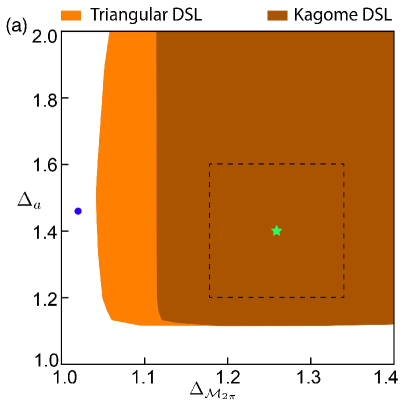
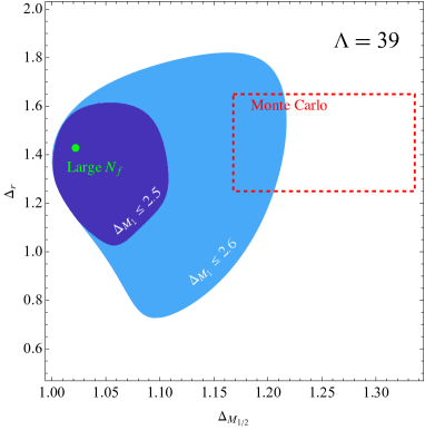
Figure 1: On the left: The allowed region in the space of dimensions of the fermion bilinear ($a$) and the monopole ($\mathcal{M}_{2\pi}$) from Ref. He:2021sto . The gap assumptions are imposed to be compatible with the conformal phase scenario on triangular lattice and the kagome lattice. The green star and dashed-line box represent the estimation and error bars from the Monte Carlo simulation, respectively, while the blue point indicates the large-$N$ estimation. On the right: The allowed region in the space of dimensions of the fermion bilinear ($\Delta_{r}$) and the monopole ($\mathcal{M}_{1}$) from Ref. Albayrak:2021xtd . Various gaps are imposed (see Figure 5 in Albayrak:2021xtd ).

Specifically, the topological charge $q=1$ monopole operator $M_{1}$ and a charge neutral operator $S_{(220)}$ must be irrelevant for the conformal phase scenario to be realized in the Kagome lattice Song2018 ; Song2018a . $\text{QED}_{3}$ has been studied using both large-$N_{f}$ expansion and Monte Carlo simulations. While Monte Carlo simulation support the CFT scenario Karthik2015 ; Karthik2016 ; Karthik2019 , large-$N$ prediction yield $\Delta_{M_{1}}\approx 2.499$ and $\Delta_{S_{(220)}}\approx 2.379$ Chester:2016wrc , which are relevant and would rule out the CFT scenario.

The bootstrap study of a single correlator of the fermion bilinear operator was initiated in Li:2018lyb , where various large-$N$ expansion results were injected into the setup. That study observed a kink moving with the dimension $\Delta_{*}$ of the first scalar in a certain representation (denoted as $T\bar{A}$ in Li:2018lyb ), and suggested that the kink may correspond to the fermionic $\text{QED}_{3}$ if $\Delta_{*}$ were fixed to the actual CFT value.

After that, two bootstrap studies He:2021sto ; Albayrak:2021xtd investigated the mixed correlators between the lowest monopole and the fermion bilinears. Strong bounds on CFT data have been obtained; see Fig. 1. Ref. He:2021sto imposed gap assumptions that are compatible with the conformal phase scenarios (specifically $\Delta_{M_{1}}\geqslant 3$ and $\Delta_{S_{(220)}}\geqslant 3$ for the Kagomé lattice). The resulting bounds are consistent with the latest Monte Carlo result but excluded certain results from large $N_{f}$ expansion. On the other hand, Ref. Albayrak:2021xtd imposed various gap assumptions inspired by the large $N_{f}$ result. Specifically it assumed $\Delta_{M_{1}}\leqslant 2.6,\Delta_{S_{(220)}}\geqslant 2.8$. They found bounds in an isolated region compatible with the large-$N$ prediction. To implement gap assumptions of the form $\Delta_{\text{min}}<\Delta<\Delta_{\text{max}}$, the work introduced a useful technique called interval positivity. In both works, the (ir)relevance of $M_{1}$ and $S_{(220)}$ is not determined by bootstrap, but inputted as an assumption, and a reliable spectrum has not been obtained. Thus the matter cannot considered to be settled.

For $N_{f}=2$ case, the work Li:2021emd bootstrapped the correlator of the lowest monopole operator. Combining this with some results from Monte Carlo simulations, Li:2021emd showed the IR phase of $N_{f}=2$ $\text{QED}_{3}$ is unlikely to be conformal.

3.2.2 Bootstrapping bosonic $\text{QED}_{3}$

Several works have bootstrapped the bosonic $\text{QED}_{3}$. One issue is how to distinguish $\text{QED}_{3}$ from non-abelian $SU(N_{c})$ gauge theories with the same number of matter field multiplets. This question was investigated in Reehorst:2020phk ; He:2021xvg . The key observation is that there are natural gaps in the spectrum that distinguish between different $N_{c}$ values. The simplest example concerns an operator of the form $\bar{\phi}^{[f_{1}}_{[c_{1}}\bar{\phi}^{f_{2}]}_{c_{2}]}{\phi}^{[c_{1}}_{[f_{3}}{\phi}^{c_{2}]}_{f_{4}]}$, where $\phi$ are the bosonic matter fields in the fundamental of $SU(N_{c})$, and $f_{i}$, $c_{i}$ are flavor and color indices respectively. This operator exists when $N_{c}\geqslant 2$, but an operator transforming in the same way under the global symmetry cannot be constructed in the abelian cases, using just four scalars without derivatives. Thus, imposing a gap in this symmetry sector, in principle, could isolate the abelian case from $N_{c}\geqslant 2$. With such a gap assumption, Ref. He:2021xvg bootstrapped the correlator of the leading scalar in $SU(N_{f})$ adjoint and found bounds in closed region for the large $N_{f}$ cases and in (2+$\epsilon$)D for small $N_{f}$. However, it’s not clear whether the closed region contains only the target theory, not anything else, and whether it could converge to a small bootstrap island at large $\Lambda$ and produce precise scalar QED spectrum.

The $N_{f}=2$ case is believed to be the simplest example of the Deconfined Quantum Critical Point (DQCP). The Monte Carlo simulations have certain conflict with the bootstrap bounds (see Ref. Poland:2018epd for a review). A possible way to reconcile the bootstrap results with the Monte Carlo is proposed in Ref. Nahum:2019fjw ; Ma:2019ysf . This work suggested a formal interpolation between the 2D $SU(2)_{k=1}$ WZW theory and the 3D Deconfined Quantum Critical Point (DQCP). With a one-loop calculation, the work found the critical dimension $d_{c}\approx 2.77$, where the theory annihilates and becomes a complex CFT, an example of the merger and annihilation scenario gorbenko2018walking ; gorbenko2018walking2 . If this scenario is correct, the bosonic QED₃ for $N_{f}=2$ does not exist in 3D as a unitary fixed point, and the DQCP phase transition is weakly first order.

This scenario may be checked via the numerical bootstrap analysis of the $SU(2)_{k=1}$ WZW theory in 2D and in non-integer $d>2$. The first 2D analysis was performed in Ohtsuki:thesis , which discovered that the WZW theory sits at a sharp kink of a single correlator bound. Then, Refs. Li:2020bnb ; He:2020azu investigated the fate of this kink in non-integer $d>2$, as well as in the case of larger $N_{f}$. Ref. He:2020azu found evidence to support the critical dimension proposed in Ref. Ma:2019ysf .

3.2.3 Bootstrapping the flavor currents

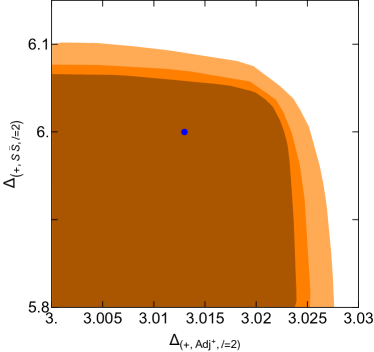
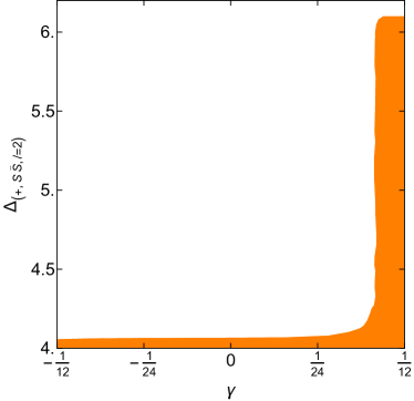
Figure 2: Feasibility bounds from bootstrapping non-abelian current. On the left: The lowest operator in the $(+,S\bar{S}$, $\ell=2)$ sector v.s. the sector $(+,Adj^{+},\ell=2)$ in $SU(100)$ CFT, where $Adj^{+}$ is the adjoint representation. $\Lambda=19,23,27$. Blue point is the large-$N$ result. On the right: $\gamma$ versus the lowest operator in the $(+,S\bar{S}$, $\ell=2)$ in $SU(100)$ CFT. $\Lambda=19$. $\gamma$ is a parameter appearing in the current, current, stress tensor 3-point function, and it obeys the conformal collider bounds $|\gamma|\leqslant 1/2$ HofmanConformalCollider2008 . In both cases, mild gaps in several sectors are imposed. The bounds are insensitive to those gap assumptions.

The existence of conserved currents is a key features of all local CFTs possessing continuous global symmetry. Global symmetry currents (referred to below as simply currents) are CFT primaries of spin 1 which are conserved and have protected scaling dimension $d-1$. In addition, OPE coefficients of currents with other primaries are constrained by Ward identities. One expects that implementing those properties in a bootstrap setup could lead to new bounds and new spectral data that cannot be accessed in setups dealing only with scalar primaries.

For the problem of bootstrapping critical gauge theories, correlators involving currents are appealing to consider for several other reasons. For the abelian gauge theories in 3D, the existence of topological current $j_{\text{top}}^{\rho}=\epsilon^{\mu\nu\rho}\partial_{\mu}A_{\nu}$ is a key feature; operators charged under this current are called monopole operators. The existence of this current could e.g. distinguish fermionic QED₃ from the free fermion theory. Below we will see other examples of how correlators of currents can help distinguishing critical gauge theories from other theories.

The bootstrap study of the four-point function of currents in 3D CFTs with a $U(1)$ symmetry was initiated in Dymarsky:2017xzb . Subsequently, the work Reehorst:2019pzi studied the 3D $O(2)$ model using mixed correlators of the $O(2)$ current and a singlet. Ref. Reehorst:2019pzi obtained several new data that was not accessible in prior scalar correlator studies of the $O(2)$ model Kos:2013tga (although Reehorst:2019pzi used some results of Kos:2013tga as an input). As already mentioned, abelian 3D gauge theories have $U(1)$ topological currents, however no features associated with these theories was observed in the bounds of Dymarsky:2017xzb ; Reehorst:2019pzi .

More recently, Ref. He:2023ewx bootstrapped for the first time the four-point functions of currents in the CFTs with a non-abelian continuous symmetry. Similar to the bosonic QED case studied in He:2021xvg , Ref. He:2023ewx proposed to impose gap assumptions on the spectrum of exchanged operators, which can be used to distinguish between different $N_{c}$ for the fermionic case, and in particular the abelian from the non-abelian cases. In fermionic $U(N_{c})$ gauge theories, an operator of the form $\bar{\psi}^{(f_{1},c_{1}}\gamma^{\mu}\psi_{(f_{2},c_{1}}\bar{\psi}^{f_{3},c_{2})}\gamma^{\nu}\psi_{f_{4},c_{2})}$, where $f_{i}$, $c_{i}$ are flavor and color indices respectively, exists only for $N_{c}\geqslant 2$. Such an operator has scaling dimension 4 in the large-$N_{f}$ limit. Thus, a gap beyond 4 in this channel could, in principle, distinguish fermionic QED from fermionic QCD. The representation to which this operator belongs is denoted in He:2023ewx as $(+,S\bar{S}$, $\ell=2)$, where $+$ denotes spacetime parity and $\ell$ is the spin. This gap could also remove the solution of Generalized Free Field (GFF), where the leading operator $(J^{\mu})^{(f_{1}}{}_{(f_{2}}(J^{\nu})^{f_{3})}{}_{f_{4})}$ has scaling dimension 4. Note that $(+,S\bar{S}$, $\ell=2)$ could be accessed already in the scalar bootstrap of Ref. He:2021sto ; Albayrak:2021xtd . However, in that setup, the GFF operator has a scaling dimension of 6. Indeed, Ref. He:2021sto found no signal of $N_{f}=4$ $\text{QED}_{3}$ in this sector. We see a clear advantage of the setup involving external currents..

By scanning over the gaps in $(+,S\bar{S}$, $\ell=2)$ and other parameters, Ref.  He:2023ewx obtained strong bounds on CFT data, and observed kinks; see Fig. 2. Large $N_{f}$ $\text{QED}_{3}$ appears to be close to some kinks. Ref. He:2023ewx also imposed stronger conditions by demanding that many operators lies within mild windows around the large-$N_{f}$ values. With such assumptions, in large $N_{f}$ cases, the bound turns into an isolated region, which does not contain any obvious known theories other than $N_{f}=4$ $\text{QED}_{3}$. However, the isolated region is not small enough to produce a precise QED spectrum. Furthermore, it’s not clear whether the closed regions could converge to a small bootstrap island at high $\Lambda$.

The discussed recent computations were allowed by the progress in the conformal block and SDP software. In the first $U(1)$ current study of Dymarsky:2017xzb , conformal block of the current correlator were computed by decomposing them into (derivatives of) scalar blocks. On the other hand, the setup in He:2023ewx produces SDPs that are much larger in size than those in Dymarsky:2017xzb and are more challenging to generate and compute. These calculations have become feasible due to the development of blocks_3d and SDPB 2.0, as discussed in Section 2.

To summarize, bootstrapping critical gauge theories remains a challenge. Various attempts on bootstrapping QED in 3D and (2+$\epsilon$)D have been made. Despite having found strong bounds in the theory space, no one has obtained a small bootstrap island that could produce precise and reliable CFT data. In future work, for a successful bootstrap analysis of QED, it might be necessary to consider larger systems of mixed correlators. One could also consider correlators involving open or closed Wilson lines, although formulating a conformal bootstrap program for these observables is a wide open problem.

3.3 Multiscalar CFTs

In this review, by a multiscalar CFT we mean an IR fixed point of a Lagrangian field theory of $N$ scalar fields with quartic interactions in the UV, which respect global symmetry $G\subset O(N)$. Physically, one is most interested in stable fixed points, i.e. possessing only one relevant singlet scalar (the mass term). For small $N$, the possible stable fixed points are limited. See Rong:2023xhz for a classification of all stable fixed points for up to five scalars, based on one-loop calculations in $d=4-\epsilon$ dimensions. Apart from the Ising and $O(N)$ CFTs, simple multiscalar CFTs include those with symmetries $\mathds{Z}_{2}^{n}\rtimes{\mathcal{S}_{n}}$ (the cubic symmetry), $\mathds{Z}_{2}\times{\mathcal{S}_{n}}$, $O(m)^{n}\rtimes{\mathcal{S}_{n}}$, and $O(m)\times O(n)$. For all these symmetry groups there exist a family of $d$-dimensional CFTs which for $d=4-\epsilon$ and $\epsilon\ll 1$ are weakly coupled and smoothly connect to the free theory for $d=4$. These families can be studied via the $\epsilon$-expansion which, when extended for $\epsilon=1$ and Borel-resummed, gives predictions for 3D CFTs. Several works have studied CFTs with these global symmetries using the conformal bootstrap. One hope of these studies is to recover the results predicted via the $\epsilon$-expansion using the non-perturbative technique (and perhaps with a better precision). In addition, one may hope to discover other CFTs having the same global symmetry (in addition to the one predicted by the $\epsilon$-expansion).

Bootstrap studies of CFTs with the cubic symmetry $\mathds{Z}_{2}^{n}\rtimes\mathcal{S}_{n}$ began with Rong:2017cow ; Stergiou:2018gjj . Bounds from a single correlator of an operator $v$ in the standard $(n-1)$-dimensional representation have been obtained, working in 3D. While some kinks were observed on the bounds, they do not correspond to “the cubic CFT”, i.e. the CFT predicted by the $\epsilon$-expansion aharony1973critical . Ref. Stergiou:2018gjj conjectured that the kink corresponds to a new CFT which they dubbed “Platonic CFT.” Refs. Kousvos:2018rhl ; Kousvos:2019hgc further investigated the conjectured Platonic CFT using four-point functions of $v,s$, where $s$ is the lowest singlet operator. Imposing that a certain operator saturate the single correlator bound, with other reasonably mild gap assumptions, they obtained an isolated allowed region.

The works of Nakayama:2014lva ; Henriksson:2020fqi studied theories with $O(m)\times O(n)$ symmetry. Kinks were observed on the bounds from a single correlator of $\phi_{ar}$ (the bifundamental representation, with $a,r$ being $O(m),O(n)$ vector indices), and they are consistent with the large $n$ expansion for $O(m)\times O(n)$ Wilson-Fisher theories at fixed $m$. Using a mixed correlator setup involving $\phi_{ar}$ and the leading singlet operator, Henriksson:2020fqi showed that the CFT can be constrained to an isolated region by demanding certain operator saturate a bound.

Similar methods were applied to the $O(m)^{n}\rtimes\mathcal{S}_{n}$ symmetry Stergiou:2019dcv ; Henriksson:2021lwn ; Kousvos:2021rar and the $U(m)\times U(n)$ symmetry Kousvos:2022ewl . Ref. Stergiou:2019dcv studied a single correlator of $\phi_{i}$, where $i=1,...,mn$ labels $n$ copies of $O(m)$ vectors transforming under $O(m)^{n}\rtimes\mathcal{S}_{n}$. Focusing on the $O(2)^{2}\rtimes\mathcal{S}_{2}$ case, Ref. Stergiou:2019dcv made interesting observations: Several materials are supposed to undergo phase transitions described by a CFT with $O(2)^{2}\rtimes\mathcal{S}_{2}$. Experiments on these phase transitions have yielded two sets of critical exponents. Surprisingly, two kinks were exhibited on the single correlator bound, which are in good agreement with the two sets of experimental data. Ref. Henriksson:2021lwn further studied the kinks at the large-$m$ limit. Ref. Kousvos:2021rar investigated a mixed correlator system involving $\phi$ and an operator $X$ that is a singlet under $O(m)$ but a fundamental representation in $\mathcal{S}_{n}$. Ref. Kousvos:2021rar found isolated regions under certain gap assumptions. However, the fate of the two possible $O(m)^{n}\rtimes\mathcal{S}_{n}$ CFTs remains inconclusive.

In conclusion, despite obtaining many strong bounds for various multiscalar CFTs, small bootstrap islands have still not yet been obtained for those theories. In an upcoming work ono2talk ; ono2 , this is achieved for the multiscalar CFTs with $O(N)\times O(2)$ global symmetry.

Outside the scope of local theories, Behan:2018hfx studied all three relevant scalars in the long-range Ising model and found a kink in the numerical bounds that corresponds to the target CFT; further interesting results on this model were obtained in Behan:2023ile .

3.4 Extraordinary phase transition in the $O(N)$ boundary CFT

Conformal defects are difficult to bootstrap using the rigorous numerical conformal bootstrap methods based on SDPs, because the OPE coefficients in the bootstrap equation involving both the bulk and the defects generally do not exhibit positivity properties. One non-rigorous method usually applied to bootstrap these systems is Gliozzi’s method Gliozzi:2013ysa , where one solves directly the truncated bootstrap equation, without assuming positivity of the OPE coefficients. However, the error in this method is not systematically controllable.

In this section, we review a recent exploration Padayasi:2021sik on bootstrapping the boundary of 3D $O(N)$ CFTs, representing a special case to which the standard SDP approach can be applied. The system under consideration is the Heisenberg model on a $d$-dimensional lattice with an infinite plane boundary at $x_{d}=0$:

$${\cal H}=-\sum_{\langle i,j\rangle}K_{i,j}\vec{S}_{i}\cdot\vec{S}_{j},$$ (2)

where $\vec{S}_{i}$ is the classical $O(N)$ spin, $\langle i,j\rangle$ denotes a pair of neighbouring sites, and $K_{i,j}=K_{1}$ when the pair is on the boundary and $K_{i,j}=K$ when the pair is in the bulk. Depending on $N$, the system exhibits different properties. An extraordinary boundary transition happens only when $N\leqslant N_{c}$. $N_{c}$ is determined by another boundary unversality class, called the normal transition. In normal transition, the crossing equation (bulk-to-boundary bootstrap equation) for two-point function of real scalars is schematically

$$1+\sum_{k}\lambda_{k}f_{\text{bulk}}(\Delta_{k},\xi)=\xi^{\Delta_{\phi}}\left(\mu_{\phi}+\sum_{n}\mu_{n}f_{\text{bry}}(\hat{\Delta}_{n},\xi)\right)$$ (3)

where $\sum_{k}$ is over the bulk operator and $\xi$ is a cross ratio for the buld/boundary scenario; $\sum_{n}$ is the sum over the boundary operators. In the case of $O(N)$ CFT, these terms will be dressed with the $O(N)$ tensor structure, which contains $N$ explicitly. Then, certain OPE coefficients, together with $N$ could determine $N_{c}$. Specifically, the extraordinary phase transition happens when the quantity $\alpha=\frac{1}{32\pi}\frac{\mu_{\sigma}}{\mu_{t}}-\frac{N-2}{2\pi}$ is positive, where $\mu_{t},\mu_{\sigma}$ are certain OPE coefficients.

The OPE coefficients in Eq. (3) are, in general, not positive. However, in this specific case, the $2+\epsilon$, large-$N$, $4-\epsilon$ calculation all show these coefficients are positive. Ref. Padayasi:2021sik also studied the system using Gliozzi’s method, which show no negativity in those OPE coefficients. The work then assumed the positivity of coefficents and formulate the problem as a SDP. It applied the standard approach to map out the feasible region in $\alpha$ vs. $N$. The work found the bound $N_{c}>3$, which is rigorous if one accepts the positivity assumptions. With the Gliozzi method, the work found $N_{c}\approx 4$, consistent with Monte Carlo results. This work is an example where the standard SDP method could be applied to study the bulk-to-boundary bootstrap equation in some situations.

4 Delaunay triangulation and surface cutting

It is a natural expectation that incorporating more and more crossing equations should increase the constraining power of the conformal bootstrap. This has been demonstrated in Kos:2014bka ; Kos:2015mba ; Kos:2016ysd , where for the first time more than one crossing equation was used. Furthermore Ref. Kos:2016ysd showed that the non-degeneracy of an isolated exchanged operator is a powerful constraint. This isolated non-degenerate operator may be one of the external operators, or an operator which is otherwise known to be non-degenerate. When the non-degeneracy condition is imposed, the contribution of an isolated operator to a crossing equation is proportional to a rank-1 positive-semidefinite matrix, parametrized by the OPE coefficients external-external-exchanged. Thus the corresponding SDPs usually depend on two classes of parameters: the scaling dimensions of the external operators and the OPE coefficients external-external-exchanged for the isolated exchanged operators. In typical bootstrap studies, one wants to map out the allowed region (i.e. the region consistent with the crossing equations) in the parameter space. For every point in the parameter space, SDPB can tell us if the point is allowed or not. We would like to perform a scan of the parameter space, running SDPB for many points, and then infer the shape of the boundary of the allowed region.

As we consider correlators involving more and more external operators, the dimension of the parameter space increases rapidly. Exploring such a high dimensional space is a major challenge for numerical bootstrap study of large correlator systems. A brute force scanning approach would suffer from the “curse of dimensionality”, as the number of SDP runs will increase exponentially with the dimension of space. Here we would like to highlight the algorithms developed in Chester:2019ifh ; Chester:2020iyt , which partially address this challenge. Using those algorithms, the cited references achieved remarkable progress on the critical exponents of 3D $O(2)$ and $O(3)$ vector models. We will now review the main ideas and these applications.

4.1 Algorithms

As mentioned above, we must perform a scan in the space of scaling dimensions times OPE coefficients. These two scanning directions are handled separately. For the scaling dimensions, one uses an adaptive sampling method, called Delaunay triangulation, to map out the boundary of the allowed region. One first computes a grid of points that contains both allowed and disallowed points, then one applies the Delaunay triangulation Delauney which finds a special set of triangles that link those points. The triangles that contain both allowed points and disallowed points are the triangles covering the boundary. The area of those triangles roughly indicates the local resolution of the boundary. One then ranks those triangles by area and samples the middle points of the largest triangles, i.e. focus on improving the regions with low resolution. This method is essentially a higher dimensional generalization of the 1D bisection method. It works well for 2D and 3D space. This was enough for the applications in Chester:2019ifh ; Chester:2020iyt . For higher dimensional space, the computations become much slower and the “curse of the dimensionality” strikes back.

As for the scan in the space of the OPE coefficients, the work Chester:2019ifh developed a novel method, called the cutting surface algorithm, which is significantly faster than the Delaunay triangulation method. Here we describe the basic idea using a low-dimensional example, and then briefly discuss the higher-dimensional case.

A non-degenerate isolated internal operator gives rise to a term in the crossing equation of the form $\lambda^{T}.\vec{V}.\lambda$ where $\lambda\in\mathbb{R}^{n}$ is the vector of its OPE coefficients with the external operators and $\vec{V}$ is a vector of $n\times n$ matrices. Given a trial point $\lambda_{1}$, we use SDPB to look for a functional $\alpha_{1}$ such that $\lambda_{1}^{T}.\alpha_{1}(\vec{V}).\lambda_{1}\geqslant 0$. If such a functional exists, the point $\lambda_{1}$ is ruled out, otherwise one concludes $\lambda_{1}$ is an allowed point. The key observation is that $\alpha_{1}$, if it exists, rules out not only $\lambda_{1}$ but also a sizable disallowed region around $\lambda_{1}$. If $\lambda$ is a 2D vector, this disallowed region can be easily found explicitly by solving the quadratic inequality $\lambda^{T}.\alpha_{1}(V).\lambda\geqslant 0$. The next trial point $\lambda_{2}$ can now be chosen outside of this disallowed region, and so on. The disallowed region, which is the union of disallowed regions of $\lambda_{1},\lambda_{2},\ldots$, quickly grows. In the end, one ends up with an allowed point, or the disallowed region covers the entire space.

When $\lambda\in\mathbb{R}^{n}$, $n\geqslant 3$, the disallowed region has to be defined implicitly by a set of quadratic inequalities $\lambda^{T}.\alpha_{i}(V).\lambda\geqslant 0$, $i=1,\ldots,k$. One decides the new trial $\lambda_{\text{next}}$ in step $k+1$ by two steps: (1) try to find a point that is outside the disallowed region, i.e. $\lambda_{\text{next}}^{T}.\alpha_{i}(V).\lambda_{\text{next}}<0$ for all $\alpha_{i}$; (2) try to move this point away from the disallowed region as much as possible. The reason for (2) is that, if the new point $\lambda_{\text{next}}$ is chosen roughly at the center of the undetermined region, the new functional $\alpha_{\text{next}}$ (if it exists) usually rules out half of that region. Since each iteration cuts off about half of the volume, the total number of steps to achieve the needed accuracy grows roughly linearly in $n$. This is a much faster performance than for the Delaunay triangulation, achievable thanks to the quadratic structure of the constraints. The step (1) is a type of problem called quadratically constrained quadratic program (QCQP), which in NP-hard in general. However for the problem at hand, Chester:2019ifh founds several heuristic approaches that work. The heuristics are not rigorous and should not be expected to solve generic QCQPs. What sets our problem apart is that one often has some idea about the expected size of the OPE coefficients, and a bounding box can then be set to constraint the space. With a suitable bounding box, those heuristics work very well, at least when the number of OPE coefficients is not too big. When the heuristics fail to find an allowed point, one declares the OPE coefficient space is ruled out. To speed up the computation, each SDP computation is “hot-started” Go:2019lke , namely one reuses of the final state of the SDP solver from the previous computation as the initial state in the new computation.

To combine Delauney triangulation with cutting surface, one proceeds as follows. First one chooses a grid of points in the space of scaling dimensions and computes the allowedness of each point, which means using the cutting surface algorithm to rule out (or find allowed) OPE coefficients inside the bounding box (at fixed scaling dimensions). Then one uses the Delaunay triangulation refine the grid in the space of scaling dimensions. This combined algorithm is suitable for 2 or 3 scaling dimensions, and a few OPE coefficients. It is implemented in both hyperion and simpleboot frameworks.

4.2 Application to the $O(2)$ model: the $\nu$ controversy resolved

The 3d $O(2)$ universality class describes critical phenomena in many physical systems and has been studied intensively both experimentally and theoretically. Experimentally, the most precise measurement of the 3d $O(2)$ critical exponents came from the study of ⁴He superfluid phase transition on the Space Shuttle Columbia in 1992 Lipa:1996zz ; Lipa:2000zz ; Lipa:2003zz . The critical exponent $\nu$ obtained from the data analysis of this experiment was $\nu^{\text{EXP}}=0.6709(1)$.

Theoretically, the simplest description in continuum file theory is given by the Lagrangian, where the mass term $m^{2}$ needs to be fine-tuned to reach the critical point:

$${\cal L}=\frac{1}{2}|\partial\vec{\phi}|^{2}+\frac{1}{2}m^{2}|\vec{\phi}|^{2}+\frac{g}{4!}|\vec{\phi}|^{4}\,,$$ (4)

where $\phi$ transforms in the fundamental representation of $O(2)$ and $s=|\vec{\phi}|^{2}$ is the leading singlet. Their scaling dimensions are related to critical exponents by

$$\Delta_{\phi}=\frac{1+\eta}{2}\,,\qquad\Delta_{s}=3-\frac{1}{\nu}.$$ (5)

They can be calculated using the renormalization group method. More accurate results however came from the Monte Carlo (MC) simulation of Hasenbusch:2019jkj , which estimated $\nu^{\text{MC}}=0.67169(7)$. Intriguingly, there is a 8$\sigma$ difference between $\nu^{\text{MC}}$ and $\nu^{\text{EXP}}$.

The bootstrap study of the 3d $O(N)$ model was initiated in Kos:2013tga by considering the correlation function $\langle\phi_{i}\phi_{j}\phi_{k}\phi_{l}\rangle$. Later, in Kos:2015mba ; Kos:2016ysd , all correlation functions of $\phi,s$ were bootstrapped, which allowed to constrain the scaling dimensions $\Delta_{\phi}$, $\Delta_{s}$ to an island, although the size of that island was not yet sufficiently small to discriminate between $\nu^{\text{MC}}$ and $\nu^{\text{EXP}}$.

Finally, Ref. Chester:2019ifh considered an even larger system of correlation functions, involving three relevant fields of this model as external operators: scalars $\phi,s$ and the charge-2 operator $t_{ij}=\phi_{i}\phi_{j}-\frac{1}{2}\delta_{ij}(\phi_{k}\phi^{k})$. Thanks to employing the cutting surface algorithm and pushing to a high derivative order, this paper could resolve the $\nu^{\text{MC}}$/$\nu^{\text{EXP}}$ puzzle, as we now describe. The assumptions of Chester:2019ifh on the spectrum are that $\phi,s,t$ are the only relevant operators in the charge-0,1,2 sectors, while the charge-3 scalars having dimension larger than 1 and all charge-4 scalars irrelevant. These assumptions are physically reasonable. Under these assumptions, Chester:2019ifh explored the parameter space spanned by 3 dimensions of $\{\phi,s,t\}$ and 3 OPE coefficient ratios $\{\lambda_{sss}/\lambda_{\phi\phi t},\lambda_{\phi\phi s}/\lambda_{\phi\phi t},\lambda_{tts}/\lambda_{\phi\phi t}\}$. The Delauney triangulation/cutting surface algorithm described above was used to scan over this 6-dimensional space efficiently. The most constraining computation was done at the derivative order $\Lambda=43$, and consumed 1.03M CPU core-hours. The results are summarized in Table 2.

CFT data	value
$\Delta_{s}$	1.51136(22)
$\Delta_{\phi}$	0.519088(22)
$\Delta_{t}$	1.23629(11)

Table 2: Results of Chester:2019ifh for the scaling dimensions of $s,\phi,t$, the leading charge 0, 1, and 2 scalars. Uncertainties in bold are rigorous.

The found $\Delta_{s}$ translates into the critical exponent $\nu$ from the conformal bootstrap: $\nu^{\text{CB}}=0.671754(\bf 99)$. The uncertainty in bold font is rigorous because it was determined from an allowed bootstrap island, which may only shrink as more and more constraints are added in future studies. This value is consistent with $\nu^{\text{MC}}$ but decisively rules out the experimental measurement $\nu^{\text{EXP}}$, indicating a flaw in the experiment or the data analysis.

4.3 Application to the $O(N)$ Gross-Neveu-Yukawa model

The Gross-Neveu-Yukawa (GNY) model with $O(N)$ symmetry is described by the following Lagrangian:

$$\mathcal{L}=\frac{1}{2}(\partial\phi)^{2}+\frac{i}{2}\psi_{i}\not{\partial}\psi_{i}+\frac{1}{2}m^{2}\phi^{2}+\frac{\lambda}{2}\phi^{4}+i\frac{g}{2}\phi\psi_{i}\psi_{i},$$ (6)

where $\phi$ is a parity-odd scalar, and $\psi$ represents $N$ Majorana fermions transforming in the vector representation of $O(N)$. The $O(N)$ singlet $\phi$ couples to $\psi_{i}$ through the Yukawa coupling term $\phi\psi_{i}\psi_{i}$. At a certain value of the mass $m$, the model becomes critical and flows to a CFT. When $N=1$, the model is the same as (1) and is expected to exhibit emergent $\mathcal{N}=1$ supersymmetry.

The large-$N$ expansion of the scaling dimensions of various operators in this model was computed in Gracey:2018fwq ; Manashov:2017rrx . Based on the large-$N$ results, some important features of the spectrum are: (1) there is only one single relevant operator, $\epsilon\sim\phi^{2}$; (2) due to the equation of motion, the leading parity-even fermion $\chi_{i}\sim\phi^{3}\psi_{i}$ has a large scaling dimension, and large-$N$ expansion predicts $\Delta_{\chi}\geqslant 4$; (3) although not obvious from the equation of motion, in large-$N$ computations, $\sigma\sim\phi$ is the only relevant parity-odd singlet for $N\geqslant 2$.

These features are suitable as input for a bootstrap study of the CFT. The work Erramilli:2022kgp conducted a bootstrap analysis on all four-point functions of $\sigma,\epsilon,\psi_{i}$ with reasonable and mild assumptions on $\Delta_{\sigma^{\prime}},\Delta_{\epsilon^{\prime}},\Delta_{\psi^{\prime}},\Delta_{\chi^{\prime}}$, where $\mathcal{O^{\prime}}$ denotes the next operator in the same sector as $\mathcal{O}$. The conformal block decomposition involving fermions was effectively computed using block_3d (Section 2.1).

To impose that $\sigma,\epsilon,\psi$ are the only operators at their scaling dimensions, one must scan over the OPE coefficients involving only external operators. Therefore, the free parameters include the scaling dimensions $\Delta_{\sigma},\Delta_{\epsilon},\Delta_{\psi}$ and the OPE coefficients $\lambda_{\psi\psi\sigma},\lambda_{\psi\psi\epsilon},\lambda_{\sigma\sigma\epsilon},\lambda_{\epsilon\epsilon\epsilon}$. Similar to Chester:2019ifh , Ref. Erramilli:2022kgp applied the Delaunay search algorithm to scan over the scaling dimensions, and the cutting-surface algorithm to scan over the three ratios of OPE coefficients. These techniques sufficed to get very interesting results which we will now describe.

For $N=1$, Erramilli:2022kgp assumed $\Delta_{\sigma^{\prime}}>2.5,\Delta_{\epsilon^{\prime}}>3,\Delta_{\psi^{\prime}}>2,\Delta_{\chi^{\prime}}>3.5$ and found an isolated region. The super-Ising island of Atanasov:2022bpi is located at the tip of this isolated region. Without assuming supersymmetry, Erramilli:2022kgp checked whether a conserved supercurrent exists in the isolated region. Near the tip, corresponding to the range of parameters in Table 1, the spin-3/2 upper bound was found to be $\Delta_{\text{SC}}<2.5003219$, very close to the exactly conserved supercurrent dimension 2.5. This implies that any CFT with these parameters must be, to an extremely high degree of precision, supersymmetric — strong evidence for the emergent supersymmetry scenario.

For $N=2,4,8$, Erramilli:2022kgp assumed $\Delta_{\sigma^{\prime}}>3,\Delta_{\epsilon^{\prime}}>3,\Delta_{\psi^{\prime}}>2,\Delta_{\chi^{\prime}}>3.5$ and found small bootstrap islands for those theories. Figure 3 shows these islands at $\Lambda=35$, and the scaling dimensions with rigorous error bars are summarized in Table 3.

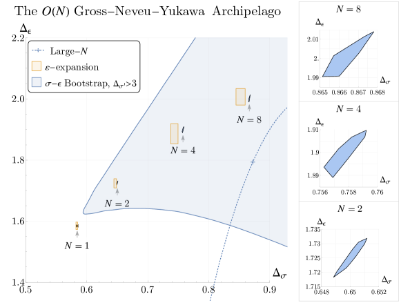
Figure 3: Bootstrap islands for $N=2,4,8$ $O(N)$ GNY model from Erramilli:2022kgp at $\Lambda=35$, projected onto the $(\Delta_{\sigma},\Delta_{\epsilon})$ plane. Dotted blue curve: perturbative estimates in the large-$N$ expansion. Orange boxes: Borel-resummations of the $(4-\epsilon)$-expansion Ihrig:2018hho . The “x” indicates the location of the $N=1$ island of Atanasov:2022bpi . Shaded region: the general $\sigma$-$\epsilon$ bootstrap bounds with the assumption $\Delta_{\sigma^{\prime}}>3$ from Atanasov:2018kqw .

	$\Delta_{\psi}$	$\Delta_{\sigma}$	$\Delta_{\epsilon}$	$\eta_{\psi}$	$\eta_{\phi}$	$\nu^{-1}$
$N=2$	$1.06861\mathbf{(12)}$	$0.6500\mathbf{(12)}$	$1.725\mathbf{(7)}$	$0.13722\mathbf{(24)}$	$0.3000\mathbf{(23)}$	$1.275\mathbf{(7)}$
$N=4$	$1.04356\mathbf{(16)}$	$0.7578\mathbf{(15)}$	$1.899\mathbf{(10)}$	$0.08712\mathbf{(32)}$	$0.5155\mathbf{(30)}$	$1.101\mathbf{(10)}$
$N=8$	$1.02119\mathbf{(5)}$	$0.8665\mathbf{(13)}$	$2.002\mathbf{(12)}$	$0.04238\mathbf{(11)}$	$0.7329\mathbf{(27)}$	$0.998\mathbf{(12)}$

Table 3: Scaling dimensions and critical exponents obtained in for the $O(N)$ GNY model, with rigorous error bars in boldface Erramilli:2022kgp .

It should be noted that there is another closely related Lagrangian

$$\mathcal{L}=\frac{1}{2}(\partial\phi)^{2}+\frac{i}{2}\psi_{i}^{A}\not{\partial}\psi_{i}^{A}+\frac{1}{2}m^{2}\phi^{2}+\frac{\lambda}{2}\phi^{4}+i\frac{g_{1}}{2}\phi(\psi_{i}^{L}\psi_{i}^{L}+\psi_{i}^{R}\psi_{i}^{R})+i\frac{g_{2}}{2}\phi(\psi_{i}^{L}\psi_{i}^{L}+\psi_{i}^{R}\psi_{i}^{R}),$$ (7)

where $i=1,\dots,\frac{N}{2}$ is an $O(N/2)$ vector index and $A=L,R$ labels two species of fermions. If $g_{1}=0,g_{2}\neq 0$, it corresponds to the $O(N)$ GNY Lagrangian (6), and its fixed point is bootstrapped in Erramilli:2022kgp . If $g_{1}\neq 0,g_{2}=0$, the model has $O(N/2)^{2}\rtimes Z_{2}$ symmetry, where $Z_{2}$ is realized by $\psi_{i}^{L}\leftrightarrow\psi_{i}^{R}$, $\phi\to-\phi$. At a critical value of mass, the $O(N/2)^{2}\rtimes Z_{2}$ GNY model is expected to flow to the “chiral Ising” universality class, which is different from the $O(N)$ GNY CFT. Various Monte Carlo simulations Huffman:2019efk ; Liu:2019xnb have studied this phase transition. There are interesting applications of this model in graphene and D-wave superconductors (see Erramilli:2022kgp for a summary). It would be interesting to see if future bootstrap studies of the $O(N/2)^{2}\rtimes Z_{2}$ GNY CFT can distinguish its critical exponents from those of the $O(N)$ GNY CFT.

5 Tiptop

In many situations, we are interested in the maximum or minimum value of a certain parameter over the allowed region. The tiptop algorithm Chester:2020iyt was designed to explore the ”tip” of a convex region. Like Delauney triangulation, tiptop usually works in pair the cutting surface algorithm: tiptop recommends new points near the tip in a direction of a certain scaling dimension, while the cutting surface algorithm is called to decide the (dis)allowedness of those points. In this section we briefly describe this algorithm and its application to the 3D $O(3)$ vector model.

5.1 The tiptop algorithm

We consider a bootstrap problem depending on $n+1$ parameters: $x\in\mathbb{R}^{n}$ and $y$. We want to know the maximum value of $y$ in the allowed region. For example, $x$ may comprise $n$ scaling dimensions and $y$ another scaling dimension we are particularly interested in. We assume the allowed region around the maximum $y$ is convex, so that as $y$ increases the allowed region of $x$ (for a fixed $y$) shrinks to zero size. The tiptop algorithm starts with some disallowed points and at least one allowed point at current $y=y_{\text{allowed}}$. Given a list of allowed, disallowed, and in-progress points (which are treated as disallowed by tiptop), it recommends one point to look at next.

To do that, tiptop first checks if the shape and the size of the allowed region at $y_{\text{allowed}}$ are well understood. An affine coordinate transformation of the $x$ space is performed, such that the region of known allowed $x$ at $y_{\text{allowed}}$ is roughly spherical. The full region of interest is then rescaled so that it is the cube $[-1,1]^{n}$. One recursively subdivides this region into cells, which are cubes of size $2^{-k}$, $k=0,1,\ldots,\min(K,47)$ , where $K$ is the first integer such that $2^{-K}$ is less than $f$ times the minimum coordinate extents of the set of allowed points, and $f$ is a user-defined parameter (e.g. $f=2$ works well). The algorithm then recommends a new point to be placed in the largest empty cell (i.e. a cell in which there is no point), which is diagonally adjacent to a cell containing allowed points.

If there is no such empty cell, the shape of allowed region at $y_{\text{allowed}}$ is considered well-understood. In this case, the algorithm recommends a new point at a higher $y$. The $x$ of the new point is roughly in the center of allowed points at $y_{\text{allowed}}$, while $y$ is half-way between $y_{\text{allowed}}$ and $y_{\text{ceiling}}$ (i.e. a bisection step). At first, $y_{\text{ceiling}}$ is a user-defined value safely larger than $y_{\max}$. After some points have been checked, $y_{\text{ceiling}}$ is the lowest disallowed $y$. If $y_{\text{allowed}}-y_{\text{ceiling}}$ is smaller than a certain user-specified value, the algorithm stops.

5.2 Application to the $O(3)$ instability problem

The $O(3)$ vector model can be defined by the Lagrangian (4) with $\phi$ in the vector representation of $O(3)$. Alternatively, the Heisenberg model on the cubic lattice with the Hamiltonian

$${\cal H}=-J\sum_{\langle x,y\rangle}\sigma_{x}\cdot\sigma_{y},$$ (8)

where $\sigma_{x}\in\mathbb{R}^{3}$ are classical spins of unit length, has the phase transition in the same universality class.

The work Chester:2020iyt bootstrapped correlators of $\phi,s,t$, which are the leading scalars in the $O(3)$ vector, singlet, rank-2 traceless symmetric tensor irreps. The bootstrap setup of the $O(3)$ CFT is similar to the $O(2)$ case except that there are more irreducible representation channels in the OPE expansion $t\times t$. Of particular interest is the operator $t_{4}$, the leading 4-index traceless symmetric tensor, appearing in this OPE.

With the assumption that $\phi,s,t$ are the only relevant scalars in their representation, the work Chester:2020iyt made two bootstrap computations. In the first computation, a conservative assumption $\Delta_{t_{4}}\geqslant 2$ was made. Then, Delauney triangulation and cutting surface were used to map out the $O(3)$ allowed island at the derivative order $\Lambda=43$. Rigorous results for the scaling dimensions of $s,\phi,t$ from this computation are given in Table 4.

CFT data	value
$\Delta_{s}$	1.59488(81)
$\Delta_{\phi}$	1.518936(61)
$\Delta_{t}$	1.20954(32)

Table 4: Conformal bootstrap results of Chester:2020iyt for the scaling dimensions of $s,\phi,t$, the leading scalars in the $O(3)$ vector, singlet, rank-2 traceless symmetric tensor irreps. Bold uncertainties are rigorous.

In the second computation, Chester:2020iyt used the tiptop algorithm to find a rigorous upper bound on $\Delta_{t_{4}}$, with the result $\Delta_{t_{4}}\leqslant 2.99056$ at $\Lambda=35$. Therefore $t_{4}$ is relevant, although very weakly so. Fig. 4 gives an idea of the progress of tiptop as it was maximizing $\Delta_{t_{4}}$.

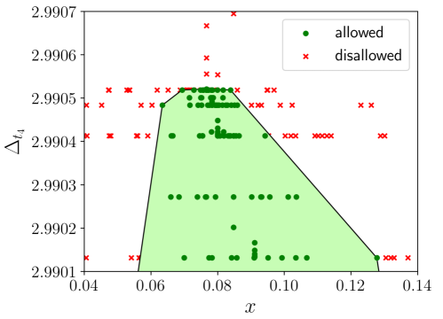
Figure 4: A two-dimensional projection of the progress of tiptop as it was maximizing $\Delta_{t_{4}}$. Figure from Chester:2020iyt .

The relevance of $t_{4}$ has phenomenological implications, which we review below. Since $t_{4}$ is relevant, the Heisenberg fixed point is unstable with respect to perturbations by (a linear combination of components of) $t_{4}$. A particularly interesting linear combination is

$$\sum_{i=1}^{3}(t_{4})_{iiii},$$ (9)

which preserves the symmetry group $B_{3}\equiv S_{3}\ltimes(\mathbb{Z}_{2})^{3}\subset O(3)$, called the cubic group. This triggers an RG flow to another fixed point called the cubic fixed point PhysRevB.8.4270 , whose symmetry group is $B_{3}$. Since $t_{4}$ is so weakly relevant, this RG flow is extremely short, and the critical exponents of the Heisenberg and cubic fixed point are very close to each other.

Previously, the (ir)relevance of $t_{4}$ was studied for many decades in perturbation theory. These studies compute the critical exponent $Y=3-\Delta_{t_{4}}$. Since $Y$ is close to zero, it is not easy to determine its sign. By year 2000, RG studies converged to the conclusion that $Y_{O(3)}>0$ at the Heisenberg fixed point, while $Y_{B_{3}}<0$ at the cubic fixed point (see Pelissetto:2000ek , Sec. 11.3, Table 33). However the error bars of these studies were significant, and the sign of $Y$ was only determined at a 2$\sigma$ level. Monte Carlo simulations improved this to 3$\sigma$ in 2011 Hasenbusch2011 . The above bootstrap result gives a rigorous proof than indeed $t_{4}$ is relevant.

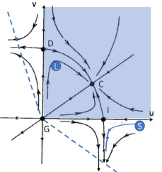
Figure 5: RG flow in the coupling plane $(u,v)$ for the case $t_{4}$ is irrelevant at the Heisenberg fixed point (I), driving the flow to the cubic fixed point (C), located at $v>0$. Figure from Aharony:2022ajv . The distance between $C$ and $I$ is exaggerated - in reality these fixed points are very close to each other. Also shown in this diagram is the schematic position of $\text{SrTiO}_{3}$ (S), flowing to a first-order transition, and $\text{LaAlO}_{3}$ (L), which is attracted to the cubic fixed point and should show a second-order transition with significant corrections to scaling.

Let us discuss phenomenological implications of the relevance of $t_{4}$. For ferromagnets this is not so important - the perturbing cubic coupling (9) will have for them a very small coefficient, having spin-orbit origin. An example when this term is important is the structural phase transition in perovskites. Perovskites like $\text{SrTiO}_{3}$ and $\text{LaAlO}_{3}$ have crystal cells preserving cubic symmetry at high temperature. As temperature decreases below a certain critical temperature $T_{c}$, the materials undergo a structural phase transition, where the lattice is stretched in a direction along an axis or a diagonal. Using the Landau theory, this phase transition can be modeled by the potential $\mu|\vec{\phi}|^{2}+u|\vec{\phi}|^{4}+v\sum_{i=1}^{3}(\phi_{i})^{4}$, where $v>0$ and $v<0$ correspond to order parameter $\phi$ breaking the cubic symmetry along an axis or a diagonal. RG studies show that the (stable as we now know for sure) cubic fixed point lies at $v>0$. The RG flow diagram is as in Fig. 5. It follows that perovskites like $\text{SrTiO}_{3}$, whose low-$T$ structure breaks the cubic symmetry along an axis, will have a first-order phase transition, while $\text{LaAlO}_{3}$ whose structure breaks cubic symmetry along a diagonal will have a second-order phase transition, in the cubic universality class Aharony:2022ajv . However, since $Y$ is so small, the flow is attracted to the cubic fixed point very slowly along the $v$ direction. Hence we expect strong corrections to scaling.

6 Navigator function

6.1 General idea

Delaunay triangulation, surface cutting and tiptop algorithms from the previous sections alleviate the curse of dimensionality in determining the shape of the allowed region. All these algorithms use SDPB in the oracle mode, testing individual points for being allowed or disallowed. The navigator function method NingSu-letter ; Reehorst:2021ykw is a radically new idea departing from the oracle philosophy. In this method a single SDPB run returns not a 0/1 information for allowed/disallowed, but a real number whose sign indicates allowed/disallowed, while the magnitude shows how far the tested point is from the allowed region boundary. This leads to even more efficient strategies for multi-parameter bootstrap studies.

As usual, we consider a bootstrap problem characterized by a finite vector of parameters $x$. Typically, $x$ includes scaling dimensions of a few operators, their OPE coefficients, and spectrum gap assumptions. Spacetime dimension $d$ and the global symmetry group parameters (such as $N$ for the $O(N)$ symmetry) may also be included in $x$.

The navigator function Reehorst:2021ykw is a continuous differentiable function $\mathcal{N}(x)$ whose sublevel set $\{x:\mathcal{N}(x)\leqslant 0\}$ coincides with the allowed region $A$. Typically this function has a nice convex shape in a neighborhood of the allowed region, with a single minimum inside it, see Fig. 6. See below for how to set up such a function and compute it using SDPB. Importantly, the gradient $\nabla\mathcal{N}(x)$ is also inexpensive to compute Reehorst:2021ykw . This is because the navigator will be given as a result of an optimization problem, and first-order variations of the objective at extremality can be found without computing the change in the minimizer.

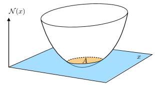
Figure 6: Schematic view of the navigator function $\mathcal{N}(x)$. The allowed region $A=\{x:\mathcal{N}(x)\leqslant 0\}$.

A typical task from which any bootstrap study starts is to find a single allowed point. This may be nontrivial if one works at a high derivative order, so that the allowed region is very small. With the navigator function, an allowed point is searched for by minimizing $\mathcal{N}(x)$ via a quasi-Newton method Reehorst:2021ykw such as BFGS wiki:BFGS . We start from an initial guess $x_{0}$ in the excluded region, and go through a sequence of points $x_{0}\rightarrow x_{1}\rightarrow x_{2}\rightarrow\cdots.$ If the allowed region is not empty, we will reach it after a finite number of steps. If, on the contrary, we reach a positive minimum of $\mathcal{N}(x)$, we conclude that the allowed region is empty.

Another typical task is to understand the shape of the allowed region. Since its boundary is the zero set of the navigator $\{x:\mathcal{N}(x)=0\}$, we can follow it by making steps tangential to the boundary and then projecting back to the boundary. This is easy to do since $\nabla\mathcal{N}(x)$ is available. For example, we can easily follow the boundary until we hit an extremal point in a certain direction Reehorst:2021ykw . This strategy supersedes the tiptop algorithm.

6.2 Existence and gradient

It is not trivial that the navigator function exists. We will explain why this is so on the prototypical example of a single correlator crossing equation:

$$\sum_{\mathcal{O}\in\phi\times\phi}p_{\phi\phi\mathcal{O}}F_{\Delta,\ell}(u,v)=0,\quad p_{\phi\phi\mathcal{O}}\geqslant 0\,.$$ (10)

We impose the constraints that

$$\ell=0:\qquad\Delta=0\ (\text{unit operator})\quad{\rm or}\quad\Delta\geqslant\Delta_{\ast},$$ (11)

while for $\ell>0$ all $\Delta$ must be at or above the unitarity bound $\Delta_{\ell}$. Eq. (10) with these constraints is the primal problem, depending on $x=(\Delta_{\phi},\Delta_{\ast})$. The dual problem is obtained by considering a linear functional $\alpha$ such that:

$$\alpha(F_{\Delta=0,\ell=0}(u,v))>0\,,$$

$$\alpha(F_{\Delta,\ell=0}(u,v))\geqslant 0\quad{\rm for}\quad\Delta\geqslant\Delta_{\ast}\,,$$ (12)

$$\alpha(F_{\Delta,\ell}(u,v))\geqslant 0\quad{\rm for}\quad\Delta\geqslant\Delta_{\ell}\,.$$

As usual, if $\alpha$ solving the dual problem exists, then there is no $p_{\phi\phi\mathcal{O}}\geqslant 0$ solving the primal problem, and $x$ is disallowed.

The navigator function is defined by solving the following modified dual problem with an objective:

$$\mathcal{N}(x)= \max_{\alpha}\alpha(F_{\Delta=0,\ell=0}(u,v))\,,\qquad\text{where}$$ (13)

$$\alpha(F_{\Delta,\ell=0}(u,v))\geqslant 0\quad{\rm for}\quad\Delta\geqslant\Delta_{\ast}\,,$$

$$\alpha(F_{\Delta,\ell}(u,v))\geqslant 0\quad{\rm for}\quad\Delta\geqslant\Delta_{\ell}\,,$$

$$\alpha(F_{{\rm norm}}(u,v))=1\,.$$

Clearly, this problem is of the form which can be handled by SDPB. The normalization vector $F_{{\rm norm}}(u,v)$ should be chosen appropriately to ensure that the navigator is finite. The criterion for this choice is that the $F_{{\rm norm}}(u,v)$ should lie strictly inside the cone $\mathcal{C}$ which is generated by all vectors $F_{\Delta,\ell}(u,v)$ allowed to appear in the crossing equation NingL4 . This naturally leads to the first navigator construction from Reehorst:2021ykw , the $\Sigma$-navigator, when one chooses:

$$F_{{\rm norm}}(u,v)=\sum_{i}F_{\Delta_{i},\ell_{i}}(u,v)$$ (14)

for a finite set of $\Delta_{i},\ell_{i}$ satisfying the spectrum constraints.

In the primal formulation, one computes the navigator as:

$$\mathcal{N}(x)=\min\lambda\,,\qquad\text{where}$$ (15)

$$\sum_{\mathcal{O}\in\phi\times\phi}p_{\phi\phi\mathcal{O}}F_{\Delta,\ell}(u,v)-\lambda F_{{\rm norm}}(u,v)=0,\quad p_{\phi\phi\mathcal{O}}\geqslant 0\,.$$

This leads to the second navigator construction from Reehorst:2021ykw , the GFF-navigator, when one chooses $-F_{{\rm norm}}(u,v)$ to be the sum of a few conformal blocks of a generalized free field (GFF) solution to crossing. The GFF navigator is naturally bounded from above by 1.

6.3 Applications

Although very recent, the navigator function method has already been applied in several studies which would be very hard or impossible with previous techniques Reehorst:2021hmp ; Sirois:2022vth ; Henriksson:2022gpa ; Chester:2022hzt . We would like to give here a brief description of these results.

6.3.1 Rigorous bounds on irrelevant operators of the 3D Ising CFT

Reehorst Reehorst:2021hmp studied the 3D Ising model CFT using the navigator function depending on 13 parameters: dimensions of 5 operators $\sigma$, $\epsilon$, $\sigma^{\prime}$, $\epsilon^{\prime}$, $T^{\prime}$ (which is the first spin-2 operator after the stress tensor), central charge $c_{T}$, and 7 OPE coefficients $\lambda_{\sigma\sigma\varepsilon}$, $\lambda_{\varepsilon\varepsilon\varepsilon}$, $\lambda_{\sigma\sigma\varepsilon^{\prime}}$, $\lambda_{\varepsilon\varepsilon\varepsilon^{\prime}}$, $\lambda_{\sigma\varepsilon\sigma^{\prime}}$, $\lambda_{\sigma\sigma T^{\prime}}$, $\lambda_{\varepsilon\varepsilon T^{\prime}}$. Imposing gaps $\Delta_{\sigma^{\prime\prime}},\Delta_{\varepsilon^{\prime\prime}},\Delta_{T^{\prime\prime}}\geqslant 6$, he determined an allowed region for the navigator function parameters. This led to rigorous two-sided bounds on all these parameters (Reehorst:2021hmp ,Table 1), for example:

$$\Delta_{\varepsilon^{\prime}}=3.82951(\mathbf{61})\qquad\text{}(\Lambda=31).$$ (16)

Previously, only four of these parameters namely $\Delta_{\sigma},\Delta_{\varepsilon},\lambda_{\sigma\sigma\varepsilon}$, $\lambda_{\varepsilon\varepsilon\varepsilon}$ Kos:2016ysd had such rigorous bounds. The bounds on other quantities were determined non-rigorously Simmons-Duffin:2016wlq by performing a partial scan over 20 points in the allowed island in the $\Delta_{\sigma},\Delta_{\varepsilon},\lambda_{\sigma\sigma\varepsilon}/\lambda_{\varepsilon\varepsilon\varepsilon}$ space, minimizing $c_{T}$ for each of them, extracting the spectrum via the extremal functional method ElShowk:2012hu , and estimating errors as one standard deviation. For $\varepsilon^{\prime}$ this non-rigorous determination gave

$$\Delta_{\varepsilon^{\prime}}=3.82968(23)\qquad\left(\text{{\cite[cite]{\@@bibref{Authors Phrase1YearPhrase2}{Simmons-Duffin:2016wlq}{\@@citephrase{(}}{\@@citephrase{)}}}}, }\Lambda=43\right).$$ (17)

We see that the rigorous determination (16), though consistent, has a larger error because it uses smaller $\Lambda$ and because the non-rigorous method is based on a very partial scan, which may further underestimate the error. Surprisingly though, for some quantities the rigorous error turns out to be somewhat smaller than the non-rigorous one, despite smaller $\Lambda$, e.g.

$$\lambda_{\varepsilon\varepsilon\varepsilon^{\prime}}=\left\{\begin{array}[]{ll}1.5362(\mathbf{12})&\left(\text{{\cite[cite]{\@@bibref{Authors Phrase1YearPhrase2}{Reehorst:2021hmp}{\@@citephrase{(}}{\@@citephrase{)}}}}, }\Lambda=19\right),\\ 1.5360(16)&\left(\text{{\cite[cite]{\@@bibref{Authors Phrase1YearPhrase2}{Simmons-Duffin:2016wlq}{\@@citephrase{(}}{\@@citephrase{)}}}}, }\Lambda=43\right).\end{array}\right.$$ (18)

As explained in Reehorst:2021hmp , in this case the non-rigorous $\lambda_{\varepsilon\varepsilon\varepsilon^{\prime}}$ determination is polluted by outlier solutions which contain not one but two nearly degenerate operators near $\Delta_{\varepsilon^{\prime}}$, sharing the OPE coefficient $\lambda_{\varepsilon\varepsilon\varepsilon^{\prime}}$ (the sharing effect Liu:2020tpf ). In the navigator function method of Reehorst:2021hmp , the operator $\varepsilon^{\prime}$ is isolated by definition, excluding the sharing effect and leading to a more robust determination of $\lambda_{\varepsilon\varepsilon\varepsilon^{\prime}}$.

6.3.2 Navigating through the $O(N)$ archipelago

Previously, Ref. Kos:2015mba studied the $O(N)$ model in $d=3$ for discrete integer values of $N=1,2,3$, …, using the scan method. Using the three-correlators setup $\langle\phi\phi\phi\phi\rangle$, $\langle\phi\phi ss\rangle$, $\langle ssss\rangle$, where $\phi,s$ are the lowest scalars in the $O(N)$ vector and singlet irreps, they isolated the $O(N)$ model in $d=3$ to islands, referred to as the $O(N)$ archipelago.

Recently, Sirois Sirois:2022vth applied the navigator method to the $O(N)$ model in the same three-correlators setup, but making $N$ and $d$ to vary continuously. The navigator function depended on four arguments $\Delta_{\phi},\Delta_{s},\lambda_{sss}/\lambda_{\phi\phi s},\Delta_{t}$, where $t$ is the lowest scalar in the $O(N)$ symmetric traceless tensor irrep. A gap up to $\Delta=d$ was imposed in these three channels, as well as gaps of $0.5$ above the stress tensor and the conserved current operators. With these assumptions, at $\Lambda=19$, Ref. Sirois:2022vth followed the islands along three continuous families in the $(d,N)$ space:

$$\left\{1\leqslant N\leqslant 3,\quad d=3\right\},$$

$$\left\{N=2,\quad 3\leqslant d\leqslant 4\right\},$$ (19)

$$\left\{N=3,\quad 3\leqslant d\leqslant 4\right\}.$$

The position and size of the islands were determined along each line and compared to the predictions from the $\epsilon$-expansion, finding good agreement.

This study adds further evidence that one should not be afraid to apply the unitary numerical conformal bootstrap method to models with noninteger $N$ and $d$ (for prior evidence in non-integer $d$ see El-Showk:2013nia ; Cappelli:2018vir ; Bonanno:2022ztf ). Indeed, while such models are nominally non-unitary Maldacena:2011jn ; Hogervorst:2014rta ; Hogervorst:2015akt , unitarity violations are secluded at very high operator dimensions, and are invisible at the currently attainable numerical accuracy. This should be true as long as $N$ and $d$ are sufficiently large.

The situation changes however when $N$ becomes too small. For example, the limit $N\rightarrow 1$ is dangerous because the symmetric traceless and antisymmetric irreps, used in the $O(N)$ model bootstrap analysis, do not exist for $N=1$ (their dimension goes to zero as $N\rightarrow 1$). Ref. Sirois:2022vth found that the island shrunk to zero size when $N\rightarrow 1^{+}$ as $d=3$ (the first family in (19)). This is because there are primary operators in the spectrum at $N>1$ whose squared OPE coefficients go linearly to zero as $N\rightarrow 1^{+}$, preventing continuation of the unitary solution to crossing to $N<1$. Numerically, Ref. Sirois:2022vth identified two such operators in the solution to crossing at $d=3$. Analytically, similar phenomena were shown to occur in the free $O(N)$ theory, and in the perturvative setting of $d=4-\varepsilon$.

6.3.3 Ising CFT as a function of $d$: spectrum continuity and level repulsion

Previosuly, the Ising CFT was studied as a function of $d\in[2,4]$ using the single-correlator setup $\langle\sigma\sigma\sigma\sigma\rangle$, identifying the position of the theory with the kink in $\Delta_{\varepsilon}$-maximization El-Showk:2013nia or in the $c_{T}$-minimization Cappelli:2018vir ; Bonanno:2022ztf . For a few intermediate values $d=3.25,3.5,3.75$, islands were found (via scans) in the three-correlator setup $\langle\sigma\sigma\sigma\sigma\rangle$, $\langle\sigma\sigma\varepsilon\varepsilon\rangle$, $\langle\varepsilon\varepsilon\varepsilon\varepsilon\rangle$ Behan:2016dtz . All these studies gave results in good agreement with the $\epsilon$-expansion.

Recently, Ref. Henriksson:2022gpa carried out a systematic study of the Ising CFT spectrum for $2.6\leqslant d\leqslant 4$ using the navigator function $\mathcal{N}(\Delta_{\sigma},\Delta_{\varepsilon},\lambda_{\varepsilon\varepsilon\varepsilon}/\lambda_{\sigma\sigma\varepsilon})$. Working at $\Lambda=30$, the low-lying spectrum was extracted applying the extremal function method at the navigator minimum for several dimensions in the $2.6\leqslant d\leqslant 4$ range.

This study led to two lessons. Firstly, it provided further evidence that the spectrum of the Ising CFT varies continuously with $d$. Secondly, their important finding was the observation of avoided level crossing between two scalar $\mathbb{Z}_{2}$-even operators $\varepsilon^{\prime\prime}$ and $\varepsilon^{\prime\prime\prime}$ which start in $d=4-\varepsilon$ with $\Delta^{\prime\prime}=6+O(\varepsilon)$ and $\Delta^{\prime\prime\prime}=8-O(\varepsilon)$. As $d$ is lowered, the lowest order $\varepsilon$-expansion predicts crossing in $d\approx 3.3$. The perturbative $\varepsilon$-expansion does not take into account non-perturbative mixing effects between operators with the same quantum numbers. Such effects are expected to lead to avoided level crossing Korchemsky:2015cyx ; Behan:2017mwi , although the precise mechanism of how this happens when deforming in $d$ is not yet clarified. Ref. Henriksson:2022gpa provided evidence for this scenario, observing that $\Delta^{\prime\prime}$ and $\Delta^{\prime\prime\prime}$ do get close to each other and then repel around $d\approx 2.78$ with minimal difference $(\Delta^{\prime\prime\prime}-\Delta^{\prime\prime})_{\min}\approx 0.136$ (see Fig. 7).

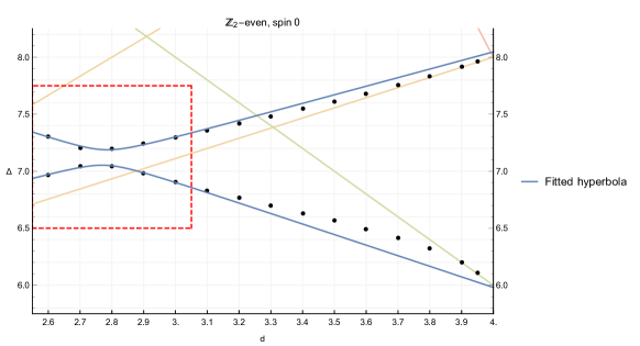
Figure 7: Observation of the level repulsion effect Henriksson:2022gpa .

In the future, it would be interesting to repeat the study of Henriksson:2022gpa at higher $\Lambda$, to determine $(\Delta^{\prime\prime\prime}-\Delta^{\prime\prime})_{\min}$ more precisely and to gain evidence that their avoided level crossing is not a finite $\Lambda$ artifact. It would also be very interesting to develop a theoretical understanding of the non-perturbative mixing effects which control $(\Delta^{\prime\prime\prime}-\Delta^{\prime\prime})_{\min}$.

6.3.4 3-state Potts model: towards the upper critical dimension

The 3-state Potts model has a second-order phase transition in $d=2$ while it has a first-order phase transition in $d=3$ Janke:1996qb . It would be interesting to get a bootstrap proof of this fact, ruling out the existence of $S_{3}$ symmetric 3D CFTs which could describe such a transition OpenProblems . It is natural to expect that the critical and the tricritical 3-state Potts CFTs merge and annihilate at some $d_{c}<3$. It would also be interesting to determine $d_{c}$.

Recently, Ref. Chester:2022hzt attacked the second question using the navigator function method. Their setup involved all 19 4pt correlation functions of external operators $\sigma,\sigma^{\prime}$, $\varepsilon$, where $\sigma,\sigma^{\prime}$ are the two relevant scalar primaries in the fundamental irrep while $\varepsilon$ is the relevant scalar singlet (assumed the only relevant scalars in these irreps). Their theory space had 10 parameters: 3 scaling dimensions of $\sigma,\sigma^{\prime}$, $\varepsilon$, and 7 ratios of OPE coefficients among them. Using the Delauney triangulation/cutting surface algorithm, they found a cone-shaped allowed region in the space of $(\Delta_{\sigma},\Delta_{\sigma^{\prime}},\Delta_{\varepsilon})$ and identifed the 3-state Potts CFT with the sharp tip of this region, see Fig. 8.

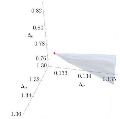
Figure 8: The cone-shaped allowed region in the space of $(\Delta_{\sigma},\Delta_{\sigma^{\prime}},\Delta_{\varepsilon})$ in $d=2$, $\Lambda=11$, whose tip (red dot) closely agrees with the exact solution of the critical 3-state Potts model Chester:2022hzt .

They also propose a similar identification for the tricritical 3-state Potts CFT, using a navigator function setup involving the second relevant singlet scalar $\varepsilon^{\prime}$ and a subset of 21 4pt correlation functions involving $\sigma,\sigma^{\prime},\varepsilon,\varepsilon^{\prime}$. In $d=2$, and at $\Lambda=11$, both identification agree very well with the exact solution.

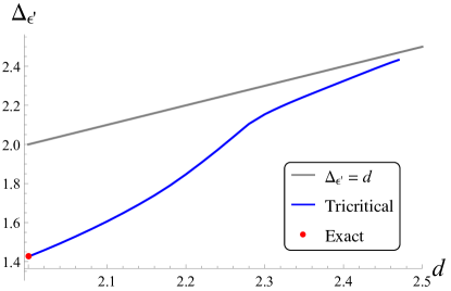
Figure 9: Tricritical $\Delta_{\varepsilon^{\prime}}$ as a function of $d$ extracted by Chester:2022hzt .

Inspired by this agreement, using the navigator function setups, Ref. Chester:2022hzt tried to track the critical and the tricritical CFTs as a function of $d>2$, assuming the same identification as in $d=2$. They wanted to see if the two CFTs come together and merge. The results of this study were not fully satisfactory. First, while the tricritical scaling dimensions varied continuously, the critical dimensions experienced an unexpected discontinuous jump at $d\approx 2.03$. Second, focusing on the cleaner tricritical curve, one could have hoped to detect $d_{c}$ as the point where $\Delta_{\varepsilon^{\prime}}(d)=d$. On general grounds, one expects a square-root behavior near this crossing Gorbenko:2018ncu :

$$\Delta_{\varepsilon^{\prime}}(d)-d_{c}\propto\sqrt{d_{c}-d}\qquad(d_{c}-d\ll 1).$$ (20)

Instead, Ref. Chester:2022hzt observed the behavior in Fig. 9. We see that $\Delta_{\varepsilon^{\prime}}$ starts approaching the $\Delta=d$ line according to the square-root law, but around $d\sim 2.28$ the behavior crosses over to a linear approach.

To overcome these difficulties, it would be desirable to find a bootstrap setup where the critical and tricritical CFT would be isolated into islands. Then $d_{c}$ could be determined from the disappearance of the islands. Unfortunately, such a setup remains elusive.

7 Skydive

In this section we will describe skydive NingSu-skydive ; Liu:2023elz , the latest dramatic improvement in the series of numerical conformal bootstrap technology improvements which started with the introduction of the navigator function.

7.1 Basic idea

The typical procedure in navigator computation involves the following steps: (1) select a point in the parameter space and generate the corresponding SDP; (2) compute the SDP to obtain the navigator function and its gradient; (3) make a move in the parameter space based on the local information from the navigator function; and then repeat the process. In the step (2), the SDP needs to be fully solved. In the technical terminology of the SDP algorithm realized in SDPB Simmons-Duffin:2015qma , an SDP is considered solved when an internal parameter $\mu$, which can be interpreted as an error measure, is reduced below a certain threshold, typically $10^{-30}$. Hot-starting often leads to the stalling of the solver if the checkpoint has a very small $\mu$. A robust strategy avoids hot-starting. A typical navigator run spends most of its time computing SDPs.

The basic idea of skydive is to optimize this approach, using an intuition that an SDP does not need to be completely solved to obtain a rough estimate of the navigator function value. Indeed, a good estimation of the navigator function can be achieved at a finite $\mu$, and such information is sufficient to indicate a good move in theory space. An ideal scenario is as follows: when the solver is far from the final optimal point, it computes the SDP until the $\mu$ is small enough to provide a reliable estimation of the navigator function, yet not so small as to cause stalling during hot-starting. Based on this estimation, the solver then moves to a new SDP nearby in the parameter space and initiates the computation of this new SDP with the previous checkpoint. In the new computation, only a few iterations are needed to obtain an acceptable estimate of the navigator function, since the checkpoint is essentially almost correct. As the solver progresses toward the final optimal point, we should methodically decrease $\mu$ to refine the estimates of the navigator function, eventually converging on the optimal point with $\mu$ below the threshold. This ideal scenario is illustrated in Figure 10.

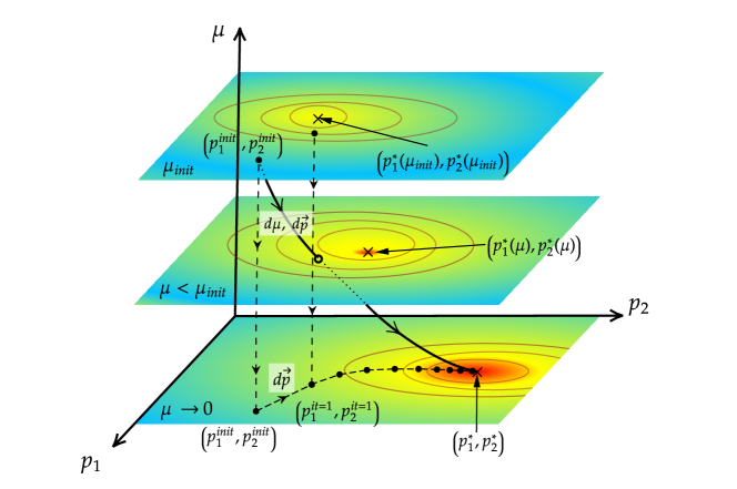
Figure 10: Original navigator function method v.s. skydiving algorithm, as illustrated in Liu:2023elz . The goal is to minimize the navigator function $\mathcal{N}(p)$ where $p=(p_{1},p_{2})$ represents parameters in theory space. In the original navigator method, we solve an SDP at fixed $(p_{1},p_{2})$ to get $\mathcal{N}(p)$ at $\mu=0$, following the vertical dashed path. Then, we update $(p_{1},p_{2})$ (suggested by the BFGS algorithm), compute another SDP starting from $\mu_{\text{init}}$, and repeat the process. On the other hand, skydive changes both $p$ and $\mu$ simultaneously, as depicted by the solid black path,converging to the same navigator minimum.

7.2 Algorithm

We will now describe the skydiving algorithm realizing this idea Liu:2023elz , which dramatically accelerates navigator-type computations.

The skydiving algorithm can be understood as an upgrade of the primal-dual interior point algorithm used in SDPB. We begin with a brief summary of the latter. The SDP can be formulated using the Lagrange function:

$$L_{\mu}(x,y,X,Y)=c^{T}x+b^{T}y-x^{T}By+\text{Tr}((X-x^{T}A_{*})Y)-\mu\log\det X,$$ (21)

where $X,Y\in\mathcal{S}^{K}$ (symmetric $K\times K$ matrices), $A_{*}=(A_{1},\ldots,A_{P})\in(\mathcal{S}^{K})^{P}$, $B\in\mathbb{(}\mathbb{R}^{n})^{P}$ are rectangular $n\times P$ matrices, and $c,x\in\mathbb{R}^{P}$, $b,y\in\mathbb{R}^{n}$ are vectors. In bootstrap applications, the constant $b,c,B,A$ quantities are related to the bootstrap conditions and conformal blocks, following the procedure in Simmons-Duffin:2015qma . In this formalism, the SDP consists in finding the stationary point of $L_{\mu}$ as $\mu\to 0$, subject to $X,Y\succeq 0$. The last term of (21) represents a barrier function which pushes us to the interior of the set $X,Y\succeq 0$. This barrier function disappears when the limit $\mu\to 0$ is taken. The primal-dual interior point algorithm solves the SDP using a variant of the Newton method with two tweaks: (1) to approach the limit $\mu\to 0$, it gradually decreases $\mu$ by replacing $\mu\to\beta\mu$ in each iteration of the Newton method, with $0<\beta<1$; (2) In each step, if the standard Newton steps $dX,dY$ violate the condition $X+dX,Y+dY\succeq 0$, the algorithm performs a partial Newtonian step, rescaling $dX,dY$ with a factor $0<\alpha<1$, to ensure that the positive semidefiniteness of $X,Y$ is preserved.

The user-chosen parameter $\beta$ is important. If $\beta$ is too small, there is a risk of stalling, a phenomenon where $\alpha$ decreases to 0, so the steps become shorter and shorter, while the solver is not at the optimal solution. Stalling indicates that the solver is too close to the boundary of the region $X,Y\succeq 0$. On this boundary we have $\det(X)=0,\det(Y)=0$. If $\mu$ is not sufficiently small, movement towards optimality is severely constrained by being close the boundary. As mentioned in Section 7.1, stalling also frequently occurs when hot-starting a new SDP (i.e. initializing the solver with given $x,y,X,Y$) using a checkpoint at small $\mu$. This is because one of the stationary conditions is $XY=\mu I$. As $\mu\to 0$, $XY\to 0$, and $X,Y$ become degenerate. From the perspective of the new SDP, the checkpoint is positioned too close to the degeneracy surface while the solution is far from optimal in the new SDP.

Suppose next that we have a family of SDP depending on a parameter $p$ (which may be multi-dimensional). For a fixed $p$ the SDP encodes the computation of a navigator function $\mathcal{N}(p)$, which we want to minimize. This means that we aim to perform optimization not only in $x,y,X,Y$ but also in $p$. We thus extend the Lagrange function to also depend on $p$:

$$L_{\mu}(x,y,X,Y,p)=c^{T}(p)x+b^{T}(p)y-x^{T}B(p)y+\text{Tr}((X-x^{T}A_{*})Y)-\mu\log\det X.$$ (22)

One might have hoped to follow the same idea as in the primal-dual interior point algorithm, i.e. using the Newton method in the space of $(x,y,X,Y,p)$ and gradually decreasing $\mu$. Unfortunately, this naive approach does not work due to very different roles played by $x,y,X,Y$ and by $p$: (1) In practical conformal bootstrap applications, the dimensions of $x,y,X,Y$ are usually much larger than those of $p$. (2) The Lagrange function depends on $x,y,X,Y$ in a smooth and convex way, but the dependence on $p$ does not have to be convex. In fact it is known that the navigator function can exhibit non-convexity (away from its minimum) and even non-smoothness. If one does try a naive Newton step treating $x,y,X,Y$ and $p$ on equal footing, performance is poor. As the solver moves through a rough landscape in $p$, fixing a constant decreasing rate $\beta$ is a bad idea and often leads to stalling. And when $x,y,X,Y$ are not stationary at a fixed $p$ and $\mu$, the predicted step in $(x,y,X,Y,p)$ is often inaccurate.

Overcome these difficulties required several new ideas introduced in Liu:2023elz . (1) The solver dynamically determines a $\beta$ based on the likelihood of stalling and may even temporarily increase $\mu$ (i.e. use $\beta>1$) when facing a higher risk of stalling. (2) The solver first finds a stationary solution for $x,y,X,Y$ at fixed $p,\mu$, and only then performs a Newton step in $p$. In other words, it attempts to optimize the “finite-$\mu$ navigator function”, defined as $N(p,\mu)=L_{\mu}(x^{*},y^{*},X^{*},Y^{*},p)$, where $x^{*},y^{*},X^{*},Y^{*}$ represents the stationary solution for a given $p,\mu$. Since the dimension of $p$ is not too large in practice, the latter optimization is much more manageable than the optimization of $L_{\mu}(x,y,X,Y,p)$. Moreover, solving the stationary solution for $x,y,X,Y$ at a fixed $p,\mu$ is, in fact, inexpensive. Ref. Liu:2023elz developed a technique that accelerates this part of the computation, typically requiring fewer than four Newton iterations to find a solution with the desired accuracy.

The above discussion would apply generically, when extremizing within a family of SDPs. However, additional difficulties arise when specializing to conformal bootstrap problems. A notable feature of the navigator function in typical conformal bootstrap studies is that it’s fairly flatness within the bootstrap island. The gradient inside and outside the island can differ by many orders of magnitude. This feature already poses a challenge in the applications of the navigator function using the original method of Reehorst:2021ykw . For the skydiving algorithm, this feature would pose a serious challenge to finding the boundary of an island, because the Lagrange function won’t detect the island (defined by $L<0$) until $\mu$ is small enough, contrary to the general idea of skydiving algorithm to move toward the optimal point at relatively big $\mu$. To overcome this challenge, Liu:2023elz proposed a modification of the Lagrangian (22) at $\mu>0$, which leads to the same allowed island and the same navigator minimum as $\mu\to 0$, but speeds up the optimization algorithm. This modification worked well in the tested examples. See Liu:2023elz for the details.

Ref. Liu:2023elz tested the skydiving algorithm on two previously studied problems involving multiple four-point functions: the 3D Ising correlators of $\sigma,\epsilon$, and the O(3) model correlators of lowest vector, singlet, and rank-2 tensor primaries. The results showed that the skydiving algorithm improved computational efficiency in these examples, compared to using the navigator function without hot-starting, by factors of 10 to 100.

The skydiving algorithm has already been used in several bootstrap studies. Notably, Ref. Rong:2023owx investigated the O(3)-symmetric correlators of $v$ (vector), $s$ (singlet), $t_{2}$ and $t_{4}$ scalar primaries (where $t_{k}$ is a traceless symmetric $k$-index irrep). The information extracted from this computation was used to perform conformal perturbation theory around the O(3) fixed point, to predict the critical exponents of the cubic fixed point. This work also numerically confirmed the large charge expansion prediction $\Delta_{Q,l}=c_{3/2}Q^{3/2}+c_{1/2}Q^{1/2}-0.094+\sqrt{\frac{l(l+1)}{2}}$ Hellerman:2015nra ; Monin:2016jmo , including for the first time the spin dependent term comparing $l=0,2$. The setup in Rong:2023owx involved the largest number of crossing equations ever explored using the numerical bootstrap: 82 equations. The computations were completed in about 10 days with the skydiving algorithm. In comparison, it would have taken more than a year using the original navigator function method of Reehorst:2021ykw (without hot-starting).

Another application of skydive was Ref. Chester:2023njo , which considered SO(5)-symmetric four-point functions of $v$, $s$, and $t_{2}$ to investigate the possibility of a conjectural scenario where DQCP is a tricritical point corresponding to a unitary CFT.

Finally, the upcoming work ono2talk ; ono2 uses skydive to study multiscalar CFTs with $O(N)\times O(2)$ global symmetry. In this work skydive is used to find the minimal value of the parameter $N$ beyond which the unitary $O(N)\times O(2)$ symmetric fixed point seizes to exist.

Clearly, the skydiving algorithm has opened new opportunities in the numerical conformal bootstrap. The algorithm of Liu:2023elz represents the first attempt at efffective optimization in the $x,y,X,Y,p$ space. Although the algorithm worked for the tested examples, its robustness needs further study, and future improvements are welcome.

8 Omissions

Unfortunately, in our review we could not describe nor mention every single numerical conformal bootstrap result obtained since the previous review Poland:2018epd . Notable omissions include: work on boundary CFTs Behan:2020nsf ; Behan:2021tcn ; solutions of the truncated bootstrap equations (Gliozzi’s method Gliozzi:2013ysa ) in situations where there is no positivity, for 4-point functions Rong:2020gbi ; Nakayama:2021zcr and for 5-point functions Poland:2023vpn ; work on superconformal field theories Bissi:2020jve ; Gimenez-Grau:2019hez ; Binder:2020ckj ; Agmon:2019imm ; Lin:2019vgi ; Gimenez-Grau:2020jrx ; Bissi:2021rei ; Liendo:2018ukf ; conformal bootstrap in situations where the spectrum is known but OPE coefficients need to be determined: Cavaglia:2021bnz ; Cavaglia:2022qpg ; Niarchos:2023lot and Picco:2019dkm ; Nivesvivat:2020gdj ; Grans-Samuelsson:2021uor ; Ribault:2022qwq ; bounds on CFT correlators Paulos:2021jxx ; work on other numerical methods such as the extremal flow method Afkhami-Jeddi:2021iuw , outer approximation and the analytic functional basis outerlimit ; Ghosh:2023onl , Machine Learning bootstrap Kantor:2021jpz , stochastic optimization LuvianoValenzuela:2022yli ; Laio:2022ayq . Regrettably, we also could not describe the work in closely related fields: the modular bootstrap for 2D CFTs Lin:2019kpn ; Lin:2021udi ; Lin:2023uvm ; Grigoletto:2021zyv ; Grigoletto:2021oho ; Chiang:2023qgo ; Fitzpatrick:2023lvh ; Huang:2019xzm ; Bae:2018qym ; Bae:2018yre ; Hartman:2019pcd ; Benjamin:2020zbs ; Benjamin:2022pnx ; Collier:2021ngi ; Afkhami-Jeddi:2020hde ; Lanzetta:2022lze ; bootstrap for Laplacian eigenvalues on surfaces Bonifacio:2020xoc ; Bonifacio:2021msa ; Kravchuk:2021akc ; Bonifacio:2021aqf ; Bonifacio:2023ban ; Gesteau:2023brw (as first shown in Kravchuk:2021akc , for hyperbolic surfaces this is extremely closely related to the conformal bootstrap). We could not describe significant progress being achieved in the sister field of the numerical S-matrix bootstrap Kruczenski:2022lot . There appeared also several other “bootstraps” where, like in the conformal bootstrap, positivity is used to get bounds on spaces of solutions (although the analogy with the conformal bootstrap is less complete due to the absence of analogues of families of conformal blocks). Those deserve separate reviews, and we list but a few entry points into the literature: the lattice model bootstrap Anderson:2016rcw ; Kazakov:2022xuh ; Cho:2022lcj , the matrix model bootstrap Lin:2020mme ; Kazakov:2021lel , the quantum mechanics bootstrap Han:2020bkb ; Lin:2023owt .

9 Discussion and outlook

In this review, we have covered some advances in numerical conformal bootstrap techniques over the last few years. The development of highly efficient software for computing conformal blocks, effectively solving SDPs, and search algorithms in theory space has been very fruitful. With these progresses in numerics, many interesting works have been done. In particular, 3D super-Ising, O(2), O(3), and GNY models have been solved to obtain high-precision critical exponents with rigorous error bars.

Many questions remain to be investigated in the future. There are many CFT targets that we would like to solve. How can we bootstrap critical gauge theories to obtain precise CFT data? Which correlators are the most constraining? How to numerically explore correlators that involve Wilson lines? How can we bootstrap multi-scalar CFTs beyond the Ising and Ising-like theories? What are the most effective gap assumptions? These are still wide open questions.

Interestingly, these questions are open even for the 2D minimal models. Can we find a systematic way to constrain minimal models into small bootstrap islands? If so, we might hope to extend these islands into non-integer dimensions $d>2$.

To bootstrap these and other targets one may think of, it is likely that we will need to further develop the bootstrap machinery to make it ever more powerful. Given a set of correlators, can we make the bootstrap bound converge faster? This question is especially crucial for correlators of large dimension operators (as is the case for critical gauge theories) since they often converge slowly in the current computational framework. There are several possibilities for acceleration:

• We may hope to accelerate the higher $\Lambda$ computation with information from a lower $\Lambda$ computation. This has been employed in the 2D chiral modular bootstrap and has achieved amazing acceleration in computation Afkhami-Jeddi:2019zci .

• In various limits, analytic understandings of the spectrum have been achieved, such as the lightcone limit and large charge limit for O(N). Combining this analytic information with numerical bootstrap should further strengthen the constraining power. A non-rigorous “hybrid bootstrap” method to combine the numerical and the lightcone information has been explored in Su:2022xnj . It would be interesting to explore more robust and rigorous methods.

• Instead of using the derivative basis, there are better bases that could converge faster. By using a better basis, amazing improvement has been achieved in the 1D CFT Paulos:2019fkw ; Ghosh:2021ruh and 2D CFT case Ghosh:2023onl . In particular in the latter work the authors observed that the bound at large external dimensions converges significantly better than what can be practically achieved with the derivative basis. Overcoming the remaining challenges to extend this method to 3D would be very useful for bootstrapping the targets mentioned in the previous paragraphs.

We remain optimistic that numerical bootstrap technology will continue seeing significant improvements in the future, and we hope that these advancements will continue yielding fascinating insights in physics questions.

Appendix A Comment on islands, isolated regions, and kinks

In this review, we used island, isolated/closed regions, and kinks to describe various bootstrap results. We would like to clarify how we use those terms.

We call an isolated allowed region in the CFT parameter space a bootstrap island of theory X if it satisfies the following conditions: (1) The gap assumptions are mild (i.e. not too close to the actual value in theory X) and/or naturally motivated (for example, by the number of relevant operators, or by equations of motion creating gaps in the spectrum, etc); (2) The isolated region is insensitive to the gap assumptions, i.e., the region doesn’t change much if the gaps are varied slightly; (3) The isolated region is small enough that it does not contain any other known theories but X. For example, we consider the 3D Ising CFT island in Figure 1 of Kos:2016ysd to satisfy these conditions. When a bootstrap island is obtained, we often can determine some CFT data with more or less rigorous error bars, by scanning over the island. One of the main goals of the conformal bootstrap program is to find the correct setups to isolate various CFTs into islands.

Kinks are sudden changes of the slope of the boundary of a feasible region. We call a kink a stable kink of theory X to mean that (1) The gap assumptions leading to the kink are mild and naturally motivated, and (2) the location of the kink is insensitive to the gap assumptions and is consistent with what is known or conjectured about the position of theory X. For example, the kink in Figure 5 of El-Showk:2012cjh is stable 3D Ising CFT kink because, when the gap changes slightly, the location remains the same, although the sharpness of the kink may change. With a stable kink, we often could make prediction on some CFT data, although the error bars may not be as rigorous as with the islands. Sometimes, one observes moving kinks, whose location changes with the gap assumptions. Those are obviously less useful than the stable kinks, but not totally useless. Indeed, in some examples, it is expected that when a certain gap is set to the actual CFT value, the CFT would precisely saturate the kink’s moving position. In these cases, bootstrap computation could make predictions on CFT data once a few pieces of information obtained using other methods are injected.

One should be careful when considering large-$N$ CFT islands. Different CFTs could have the same CFT data in the $N\to\infty$ limit. Therefore, in the theory space, there could be multiple solutions that are very close to each other at large-$N$, which may not be easily distinguishable by numerical bootstrap. These solutions may show a significant split when $N$ becomes small. Consequently, apparent success at large-$N$ does not automatically translate to success at smaller $N$. For example, in the case of the bosonic QED₃ feasible region shown in FIG. 3 of He:2021xvg , the region is closed for sufficiently large-$N$, but not at small $N$. It’s unclear whether this is purely due to a convergence issue or if there are several CFTs satisfying the imposed conditions.

Even though the ultimate goal of the conformal bootstrap program is to solve CFTs, for many target theories, it’s not yet clear how to obtain islands or stable kinks. In those cases, people compute generic bounds, while the target CFTs are not on the boundary of the bounds. These bootstrap bound are also very valuable, since sufficiently strong bounds could offer insight into related physics questions (for example, as in the case of DQCP, reviewed in Section E of Poland:2018epd ).

References

- (1) D. Poland, S. Rychkov, and A. Vichi, “The Conformal Bootstrap: Theory, Numerical Techniques, and Applications,” Rev. Mod. Phys. 91 no. 1, (2019) 15002, arXiv:1805.04405 [hep-th].
- (2) R. Rattazzi, V. S. Rychkov, E. Tonni, and A. Vichi, “Bounding scalar operator dimensions in 4D CFT,” JHEP 0812 (2008) 031, arXiv:0807.0004 [hep-th].
- (3) D. Poland and D. Simmons-Duffin, “Snowmass White Paper: The Numerical Conformal Bootstrap,” in Snowmass 2021. arXiv:2203.08117 [hep-th].
- (4) W. Landry and D. Simmons-Duffin, “Scaling the semidefinite program solver SDPB,” arXiv:1909.09745 [hep-th].
- (5) D. Simmons-Duffin, “A Semidefinite Program Solver for the Conformal Bootstrap,” JHEP 06 (2015) 174, arXiv:1502.02033 [hep-th].
- (6) S. El-Showk, M. F. Paulos, D. Poland, S. Rychkov, D. Simmons-Duffin, and A. Vichi, “Solving the 3D Ising Model with the Conformal Bootstrap,” Phys. Rev. D86 (2012) 025022, arXiv:1203.6064 [hep-th].
- (7) S. El-Showk, M. F. Paulos, D. Poland, S. Rychkov, D. Simmons-Duffin, and A. Vichi, “Solving the 3d Ising Model with the Conformal Bootstrap II. c-Minimization and Precise Critical Exponents,” J. Stat. Phys. 157 (2014) 869, arXiv:1403.4545 [hep-th].
- (8) C. Behan, P. Kravchuk, W. Landry, and D. Simmons-Duffin, “scalar_blocks,” 2019. https://gitlab.com/bootstrapcollaboration/scalar_blocks.
- (9) R. S. Erramilli, L. V. Iliesiu, and P. Kravchuk, “Recursion relation for general 3d blocks,” JHEP 12 (2019) 116, arXiv:1907.11247 [hep-th].
- (10) R. S. Erramilli, L. V. Iliesiu, P. Kravchuk, W. Landry, D. Poland, and D. Simmons-Duffin, “blocks_3d: software for general 3d conformal blocks,” JHEP 11 (2021) 006, arXiv:2011.01959 [hep-th].
- (11) D. Simmons-Duffin. https://github.com/davidsd/hyperion.
- (12) N. Su. https://gitlab.com/bootstrapcollaboration/simpleboot.
- (13) M. F. Paulos, “JuliBootS: a hands-on guide to the conformal bootstrap,” arXiv:1412.4127 [hep-th].
- (14) C. Behan, “PyCFTBoot: A flexible interface for the conformal bootstrap,” Commun. Comput. Phys. 22 no. 1, (2017) 1–38, arXiv:1602.02810 [hep-th].
- (15) T. Ohtsuki. https://github.com/tohtsky/cboot.
- (16) M. Go and Y. Tachikawa, “autoboot: A generator of bootstrap equations with global symmetry,” JHEP 06 (2019) 084, arXiv:1903.10522 [hep-th].
- (17) M. Go, “An Automated Generation of Bootstrap Equations for Numerical Study of Critical Phenomena,” arXiv:2006.04173 [hep-th].
- (18) F. Kos, D. Poland, and D. Simmons-Duffin, “Bootstrapping Mixed Correlators in the 3D Ising Model,” JHEP 11 (2014) 109, arXiv:1406.4858 [hep-th].
- (19) T. Grover, D. N. Sheng, and A. Vishwanath, “Emergent Space-Time Supersymmetry at the Boundary of a Topological Phase,” Science 344 no. 6181, (2014) 280–283, arXiv:1301.7449 [cond-mat.str-el].
- (20) D. Bashkirov, “Bootstrapping the SCFT in three dimensions,” arXiv:1310.8255 [hep-th].
- (21) L. Iliesiu, F. Kos, D. Poland, S. S. Pufu, D. Simmons-Duffin, and R. Yacoby, “Bootstrapping 3D Fermions,” JHEP 03 (2016) 120, arXiv:1508.00012 [hep-th].
- (22) J. Rong and N. Su, “Bootstrapping the minimal = 1 superconformal field theory in three dimensions,” JHEP 06 (2021) 154, arXiv:1807.04434 [hep-th].
- (23) A. Atanasov, A. Hillman, and D. Poland, “Bootstrapping the Minimal 3D SCFT,” JHEP 11 (2018) 140, arXiv:1807.05702 [hep-th].
- (24) N. Zerf, L. N. Mihaila, P. Marquard, I. F. Herbut, and M. M. Scherer, “Four-loop critical exponents for the Gross-Neveu-Yukawa models,” Phys. Rev. D 96 no. 9, (2017) 096010, arXiv:1709.05057 [hep-th].
- (25) J. Rong and N. Su, “Bootstrapping the Wess-Zumino models in three dimensions,” arXiv:1910.08578 [hep-th].
- (26) A. Atanasov, A. Hillman, D. Poland, J. Rong, and N. Su, “Precision bootstrap for the = 1 super-Ising model,” JHEP 08 (2022) 136, arXiv:2201.02206 [hep-th].
- (27) S. Gukov, “RG Flows and Bifurcations,” Nucl. Phys. B 919 (2017) 583–638, arXiv:1608.06638 [hep-th].
- (28) T. Senthil, A. Vishwanath, L. Balents, S. Sachdev, and M. P. A. Fisher, “Deconfined Quantum Critical Points,” Science 303 no. 5663, (2004) 1490–1494, arXiv:cond-mat/0311326.
- (29) T. Senthil, L. Balents, S. Sachdev, A. Vishwanath, and M. P. A. Fisher, “Quantum criticality beyond the landau-ginzburg-wilson paradigm,” Phys. Rev. B 70 (Oct, 2004) 144407. http://link.aps.org/doi/10.1103/PhysRevB.70.144407.
- (30) M. Hermele, T. Senthil, and M. P. A. Fisher, “Algebraic spin liquid as the mother of many competing orders,” Physical Review B 72 no. 10, (2005) .
- (31) X.-Y. Song, Y.-C. He, A. Vishwanath, and C. Wang, “From spinon band topology to the symmetry quantum numbers of monopoles in Dirac spin liquids,” Phys. Rev. X 10 no. 1, (2020) 011033, arXiv:1811.11182 [cond-mat.str-el].
- (32) X.-Y. Song, C. Wang, A. Vishwanath, and Y.-C. He, “Unifying Description of Competing Orders in Two Dimensional Quantum Magnets,” Nature Commun. 10 no. 1, (2019) 4254, arXiv:1811.11186 [cond-mat.str-el].
- (33) S. M. Chester and S. S. Pufu, “Towards bootstrapping QED3,” JHEP 08 (2016) 019, arXiv:1601.03476 [hep-th].
- (34) S. M. Chester, L. V. Iliesiu, M. Mezei, and S. S. Pufu, “Monopole Operators in Chern-Simons-Matter Theories,” JHEP 05 (2018) 157, arXiv:1710.00654 [hep-th].
- (35) Y. Nakayama and T. Ohtsuki, “Conformal Bootstrap Dashing Hopes of Emergent Symmetry,” Phys. Rev. Lett. 117 no. 13, (2016) 131601, arXiv:1602.07295 [cond-mat.str-el].
- (36) L. Iliesiu, “Talk at Simons Center for Geometry and Physics: Bootstrapping the Néel-VBS quantum phase transition,” November, 2018.
- (37) Z. Li, “Conformality and self-duality of QED3,” Phys. Lett. B 831 (2022) 137192, arXiv:2107.09020 [hep-th].
- (38) Y.-C. He, M. P. Zaletel, M. Oshikawa, and F. Pollmann, “Signatures of Dirac Cones in a DMRG Study of the Kagome Heisenberg Model,” Phys. Rev. X 7 (2017) 031020.
- (39) S. Hu, W. Zhu, S. Eggert, and Y.-C. He, “Dirac Spin Liquid on the Spin-1 /2 Triangular Heisenberg Antiferromagnet,” Physical Review Letters 123 no. 20, (Nov., 2019) 207203, arXiv:1905.09837 [cond-mat.str-el].
- (40) Y.-C. He, J. Rong, and N. Su, “Conformal bootstrap bounds for the Dirac spin liquid and Stiefel liquid,” SciPost Phys. 13 no. 2, (2022) 014, arXiv:2107.14637 [cond-mat.str-el].
- (41) S. Albayrak, R. S. Erramilli, Z. Li, D. Poland, and Y. Xin, “Bootstrapping =4 conformal QED3,” Phys. Rev. D 105 no. 8, (2022) 085008, arXiv:2112.02106 [hep-th].
- (42) X.-Y. Song, Y.-C. He, A. Vishwanath, and C. Wang, “From Spinon Band Topology to the Symmetry Quantum Numbers of Monopoles in Dirac Spin Liquids,” Phys. Rev. X 10 (Feb, 2020) 011033.
- (43) X.-Y. Song, C. Wang, A. Vishwanath, and Y.-C. He, “Unifying description of competing orders in two-dimensional quantum magnets,” Nature Communications 10 (Sept., 2019) 4254, arXiv:1811.11186 [cond-mat.str-el].
- (44) N. Karthik and R. Narayanan, “No evidence for bilinear condensate in parity-invariant three-dimensional QED with massless fermions,” Phys.Rev.D 93 no. 4, (2016) 045020, arXiv:1512.02993 [hep-lat].
- (45) N. Karthik and R. Narayanan, “Scale invariance of parity-invariant three-dimensional QED,” Phys.Rev.D 94 no. 6, (2016) 065026, arXiv:1606.04109 [hep-th].
- (46) N. Karthik and R. Narayanan, “Numerical determination of monopole scaling dimension in parity-invariant three-dimensional noncompact QED,” Phys.Rev.D 100 no. 5, (2019) 054514, arXiv:1908.05500 [hep-lat].
- (47) Z. Li, “Solving QED3 with Conformal Bootstrap,” arXiv:1812.09281 [hep-th].
- (48) M. Reehorst, M. Refinetti, and A. Vichi, “Bootstrapping traceless symmetric scalars,” SciPost Phys. 14 no. 4, (2023) 068, arXiv:2012.08533 [hep-th].
- (49) Y.-C. He, J. Rong, and N. Su, “A roadmap for bootstrapping critical gauge theories: decoupling operators of conformal field theories in dimensions,” SciPost Phys. 11 (2021) 111, arXiv:2101.07262 [hep-th].
- (50) A. Nahum, “Note on Wess-Zumino-Witten models and quasiuniversality in 2+1 dimensions,” Phys. Rev. B 102 no. 20, (2020) 201116, arXiv:1912.13468 [cond-mat.str-el].
- (51) R. Ma and C. Wang, “Theory of deconfined pseudocriticality,” Phys. Rev. B 102 no. 2, (2020) 020407, arXiv:1912.12315 [cond-mat.str-el].
- (52) V. Gorbenko, S. Rychkov, and B. Zan, “Walking, weak first-order transitions, and complex CFTs,” Journal of High Energy Physics 2018 no. 10, (Oct, 2018) 108, arXiv:1807.11512 [hep-th].
- (53) V. Gorbenko, S. Rychkov, and B. Zan, “Walking, Weak first-order transitions, and Complex CFTs II. Two-dimensional Potts model at ,” SciPost Physics 5 no. 5, (Nov, 2018) 050, arXiv:1808.04380 [hep-th].
- (54) T. Ohtsuki, Applied Conformal Bootstrap. PhD thesis, University of Tokyo, 2016.
- (55) Z. Li and D. Poland, “Searching for gauge theories with the conformal bootstrap,” JHEP 03 (2021) 172, arXiv:2005.01721 [hep-th].
- (56) Y.-C. He, J. Rong, and N. Su, “Non-Wilson-Fisher kinks of numerical bootstrap: from the deconfined phase transition to a putative new family of CFTs,” SciPost Phys. 10 no. 5, (2021) 115, arXiv:2005.04250 [hep-th].
- (57) D. M. Hofman and J. Maldacena, “Conformal collider physics: energy and charge correlations,” Journal of High Energy Physics 2008 no. 5, (May, 2008) 012, arXiv:0803.1467 [hep-th].
- (58) A. Dymarsky, J. Penedones, E. Trevisani, and A. Vichi, “Charting the space of 3D CFTs with a continuous global symmetry,” JHEP 05 (2019) 098, arXiv:1705.04278 [hep-th].
- (59) M. Reehorst, E. Trevisani, and A. Vichi, “Mixed Scalar-Current bootstrap in three dimensions,” arXiv:1911.05747 [hep-th].
- (60) F. Kos, D. Poland, and D. Simmons-Duffin, “Bootstrapping the vector models,” JHEP 06 (2014) 091, arXiv:1307.6856 [hep-th].
- (61) Y.-C. He, J. Rong, N. Su, and A. Vichi, “Non-Abelian currents bootstrap,” arXiv:2302.11585 [hep-th].
- (62) J. Rong and S. Rychkov, “Classifying irreducible fixed points of five scalar fields in perturbation theory,” arXiv:2306.09419 [hep-th].
- (63) J. Rong and N. Su, “Scalar CFTs and Their Large N Limits,” JHEP 09 (2018) 103, arXiv:1712.00985 [hep-th].
- (64) A. Stergiou, “Bootstrapping hypercubic and hypertetrahedral theories in three dimensions,” JHEP 05 (2018) 035, arXiv:1801.07127 [hep-th].
- (65) A. Aharony, “Critical Behavior of Anisotropic Cubic Systems,” Phys. Rev. B 8 (1973) 4270–4273.
- (66) S. R. Kousvos and A. Stergiou, “Bootstrapping Mixed Correlators in Three-Dimensional Cubic Theories,” SciPost Phys. 6 no. 3, (2019) 035, arXiv:1810.10015 [hep-th].
- (67) S. R. Kousvos and A. Stergiou, “Bootstrapping Mixed Correlators in Three-Dimensional Cubic Theories II,” SciPost Phys. 8 no. 6, (2020) 085, arXiv:1911.00522 [hep-th].
- (68) Y. Nakayama and T. Ohtsuki, “Approaching the conformal window of symmetric Landau-Ginzburg models using the conformal bootstrap,” Phys.Rev. D89 no. 12, (2014) 126009, arXiv:1404.0489 [hep-th].
- (69) J. Henriksson, S. R. Kousvos, and A. Stergiou, “Analytic and Numerical Bootstrap of CFTs with Global Symmetry in 3D,” SciPost Phys. 9 no. 3, (2020) 035, arXiv:2004.14388 [hep-th].
- (70) A. Stergiou, “Bootstrapping MN and Tetragonal CFTs in Three Dimensions,” SciPost Phys. 7 (2019) 010, arXiv:1904.00017 [hep-th].
- (71) J. Henriksson and A. Stergiou, “Perturbative and Nonperturbative Studies of CFTs with MN Global Symmetry,” SciPost Phys. 11 (2021) 015, arXiv:2101.08788 [hep-th].
- (72) S. R. Kousvos and A. Stergiou, “Bootstrapping mixed MN correlators in 3D,” SciPost Phys. 12 no. 6, (2022) 206, arXiv:2112.03919 [hep-th].
- (73) S. R. Kousvos and A. Stergiou, “CFTs with global symmetry in 3D and the chiral phase transition of QCD,” SciPost Phys. 15 no. 2, (2023) 075, arXiv:2209.02837 [hep-th].
- (74) M. Reehorst and B. Sirois, “Bootstrapping frustrated magnets: model,”. Talk at Bootstrap 2023, Saõ Paulo, Brazil, June 30, 2023.
- (75) M. Reehorst, S. Rychkov, B. Sirois, and B. C. van Rees, “Bootstrapping frustrated magnets: the fate of the chiral universality class,”. to appear.
- (76) C. Behan, “Bootstrapping the long-range Ising model in three dimensions,” J. Phys. A52 no. 7, (2019) 075401, arXiv:1810.07199 [hep-th].
- (77) C. Behan, E. Lauria, M. Nocchi, and P. van Vliet, “Analytic and numerical bootstrap for the long-range Ising model,” arXiv:2311.02742 [hep-th].
- (78) F. Gliozzi, “More constraining conformal bootstrap,” Phys.Rev.Lett. 111 (2013) 161602, arXiv:1307.3111.
- (79) J. Padayasi, A. Krishnan, M. A. Metlitski, I. A. Gruzberg, and M. Meineri, “The extraordinary boundary transition in the 3d O(N) model via conformal bootstrap,” SciPost Phys. 12 no. 6, (2022) 190, arXiv:2111.03071 [cond-mat.stat-mech].
- (80) F. Kos, D. Poland, D. Simmons-Duffin, and A. Vichi, “Bootstrapping the O(N) Archipelago,” JHEP 11 (2015) 106, arXiv:1504.07997 [hep-th].
- (81) F. Kos, D. Poland, D. Simmons-Duffin, and A. Vichi, “Precision Islands in the Ising and Models,” JHEP 08 (2016) 036, arXiv:1603.04436 [hep-th].
- (82) S. M. Chester, W. Landry, J. Liu, D. Poland, D. Simmons-Duffin, N. Su, and A. Vichi, “Carving out OPE space and precise model critical exponents,” JHEP 06 (2020) 142, arXiv:1912.03324 [hep-th].
- (83) S. M. Chester, W. Landry, J. Liu, D. Poland, D. Simmons-Duffin, N. Su, and A. Vichi, “Bootstrapping Heisenberg magnets and their cubic instability,” Phys. Rev. D 104 no. 10, (2021) 105013, arXiv:2011.14647 [hep-th].
- (84) Wikipedia, “Delaunay triangulation.”.
- (85) S. M. Chester and N. Su, “Upper critical dimension of the 3-state Potts model,” arXiv:2210.09091 [hep-th].
- (86) J. A. Lipa, D. R. Swanson, J. A. Nissen, T. C. P. Chui, and U. E. Israelsson, “Heat Capacity and Thermal Relaxation of Bulk Helium very near the Lambda Point,” Phys. Rev. Lett. 76 (1996) 944–947.
- (87) J. A. Lipa, D. R. Swanson, J. A. Nissen, Z. K. Geng, P. R. Williamson, D. A. Stricker, T. C. P. Chui, U. E. Israelsson, and M. Larson, “Specific Heat of Helium Confined to a 57- mum Planar Geometry near the Lambda Point,” Phys. Rev. Lett. 84 (2000) 4894–4897.
- (88) J. Lipa, J. Nissen, D. Stricker, D. Swanson, and T. Chui, “Specific heat of liquid helium in zero gravity very near the lambda point,” Phys.Rev. B68 (2003) 174518.
- (89) M. Hasenbusch, “Monte Carlo study of an improved clock model in three dimensions,” Phys. Rev. B 100 no. 22, (2019) 224517, arXiv:1910.05916 [cond-mat.stat-mech].
- (90) J. A. Gracey, “Fermion bilinear operator critical exponents at in the QED-Gross-Neveu universality class,” Phys. Rev. D 98 no. 8, (2018) 085012, arXiv:1808.07697 [hep-th].
- (91) A. N. Manashov and M. Strohmaier, “Correction exponents in the Gross–Neveu–Yukawa model at ,” Eur. Phys. J. C 78 no. 6, (2018) 454, arXiv:1711.02493 [hep-th].
- (92) R. S. Erramilli, L. V. Iliesiu, P. Kravchuk, A. Liu, D. Poland, and D. Simmons-Duffin, “The Gross-Neveu-Yukawa archipelago,” JHEP 02 (2023) 036, arXiv:2210.02492 [hep-th].
- (93) B. Ihrig, L. N. Mihaila, and M. M. Scherer, “Critical behavior of Dirac fermions from perturbative renormalization,” Phys. Rev. B 98 no. 12, (2018) 125109, arXiv:1806.04977 [cond-mat.str-el].
- (94) E. Huffman and S. Chandrasekharan, “Fermion-bag inspired Hamiltonian lattice field theory for fermionic quantum criticality,” Phys. Rev. D 101 no. 7, (2020) 074501, arXiv:1912.12823 [cond-mat.str-el].
- (95) Y. Liu, W. Wang, K. Sun, and Z. Y. Meng, “Designer Monte Carlo simulation for the Gross-Neveu-Yukawa transition,” Phys. Rev. B 101 no. 6, (2020) 064308, arXiv:1910.07430 [cond-mat.stat-mech].
- (96) A. Aharony, “Critical behavior of anisotropic cubic systems,” Phys. Rev. B 8 (1973) 4270–4273.
- (97) A. Pelissetto and E. Vicari, “Critical phenomena and renormalization-group theory,” Phys. Rept. 368 (2002) 549–727, arXiv:cond-mat/0012164.
- (98) M. Hasenbusch and E. Vicari, “Anisotropic perturbations in three-dimensional O(N)-symmetric vector models,” Phys. Rev. B 84 no. 12, (2011) 125136, arXiv:1108.0491 [cond-mat.stat-mech].
- (99) M. Hasenbusch, “Cubic fixed point in three dimensions: Monte Carlo simulations of the 4 model on the simple cubic lattice,” Phys. Rev. B 107 no. 2, (2023) 024409, arXiv:2211.16170 [cond-mat.stat-mech].
- (100) J. Rong and N. Su, “From O(3) to Cubic CFT: Conformal Perturbation and the Large Charge Sector,” arXiv:2311.00933 [hep-th].
- (101) A. Aharony, O. Entin-Wohlman, and A. Kudlis, “Different critical behaviors in cubic to trigonal and tetragonal perovskites,” Phys. Rev. B 105 (2022) 104101, arXiv:2201.08252 [cond-mat.stat-mech].
- (102) N. Su, “The Indicator , Letter to Slava Rychkov (March 7, 2020),”.
- (103) M. Reehorst, S. Rychkov, D. Simmons-Duffin, B. Sirois, N. Su, and B. van Rees, “Navigator Function for the Conformal Bootstrap,” SciPost Phys. 11 (2021) 072, arXiv:2104.09518 [hep-th].
- (104) Wikipedia, “Broyden–Fletcher–Goldfarb–Shanno algorithm.”.
- (105) N. Su, “Semidefinite program and the navigator function,”. Mini-Course of Numerical Conformal Bootstrap, Lecture 4, April 27, 2023.
- (106) M. Reehorst, “Rigorous bounds on irrelevant operators in the 3d Ising model CFT,” JHEP 09 (2022) 177, arXiv:2111.12093 [hep-th].
- (107) B. Sirois, “Navigating through the O(N) archipelago,” SciPost Phys. 13 no. 4, (2022) 081, arXiv:2203.11597 [hep-th].
- (108) J. Henriksson, S. R. Kousvos, and M. Reehorst, “Spectrum continuity and level repulsion: the Ising CFT from infinitesimal to finite ,” JHEP 02 (2023) 218, arXiv:2207.10118 [hep-th].
- (109) D. Simmons-Duffin, “The Lightcone Bootstrap and the Spectrum of the 3d Ising CFT,” JHEP 03 (2017) 086, arXiv:1612.08471 [hep-th].
- (110) S. El-Showk and M. F. Paulos, “Bootstrapping Conformal Field Theories with the Extremal Functional Method,” Phys. Rev. Lett. 111 no. 24, (2013) 241601, arXiv:1211.2810 [hep-th].
- (111) J. Liu, D. Meltzer, D. Poland, and D. Simmons-Duffin, “The Lorentzian inversion formula and the spectrum of the 3d O(2) CFT,” JHEP 09 (2020) 115, arXiv:2007.07914 [hep-th]. [Erratum: JHEP 01, 206 (2021)].
- (112) S. El-Showk, M. Paulos, D. Poland, S. Rychkov, D. Simmons-Duffin, and A. Vichi, “Conformal Field Theories in Fractional Dimensions,” Phys. Rev. Lett. 112 (2014) 141601, arXiv:1309.5089 [hep-th].
- (113) A. Cappelli, L. Maffi, and S. Okuda, “Critical Ising Model in Varying Dimension by Conformal Bootstrap,” JHEP 01 (2019) 161, arXiv:1811.07751 [hep-th].
- (114) C. Bonanno, A. Cappelli, M. Kompaniets, S. Okuda, and K. J. Wiese, “Benchmarking the Ising Universality Class in dimensions,” SciPost Phys. 14 (2023) 135, arXiv:2210.03051 [hep-th].
- (115) J. Maldacena and A. Zhiboedov, “Constraining Conformal Field Theories with A Higher Spin Symmetry,” J.Phys. A46 (2013) 214011, arXiv:1112.1016 [hep-th].
- (116) M. Hogervorst, S. Rychkov, and B. C. van Rees, “Truncated conformal space approach in d dimensions: A cheap alternative to lattice field theory?,” Phys. Rev. D 91 (2015) 025005, arXiv:1409.1581 [hep-th].
- (117) M. Hogervorst, S. Rychkov, and B. C. van Rees, “Unitarity violation at the Wilson-Fisher fixed point in 4- dimensions,” Phys. Rev. D 93 no. 12, (2016) 125025, arXiv:1512.00013 [hep-th].
- (118) J. Golden and M. F. Paulos, “No unitary bootstrap for the fractal Ising model,” JHEP 03 (2015) 167, arXiv:1411.7932 [hep-th].
- (119) G. P. Korchemsky, “On level crossing in conformal field theories,” JHEP 03 (2016) 212, arXiv:1512.05362 [hep-th].
- (120) C. Behan, “Conformal manifolds: ODEs from OPEs,” JHEP 03 (2018) 127, arXiv:1709.03967 [hep-th].
- (121) W. Janke and R. Villanova, “Three-dimensional three state Potts model revisited with new techniques,” Nucl. Phys. B 489 (1997) 679–696, arXiv:hep-lat/9612008.
- (122) S. Rychkov, “Open Problems in Conformal Bootstrap. Problem 1: Bootstrap proof of first-order transitions?,”. 2020.
- (123) J. Lee and J. M. Kosterlitz, “Three-dimensional q-state Potts model: Monte Carlo study near ,” Phys. Rev. B 43 (1991) 1268–1271.
- (124) V. Gorbenko, S. Rychkov, and B. Zan, “Walking, Weak first-order transitions, and Complex CFTs,” JHEP 10 (2018) 108, arXiv:1807.11512 [hep-th].
- (125) N. Su, “Skydiving to Bootstrap Islands: an Algorithm for Dynamically Constrained SDP,”. Talk at the 2022 Collaboration on the Nonperturbative Bootstrap Annual Meeting (November 10-11, 2022).
- (126) A. Liu, D. Simmons-Duffin, N. Su, and B. C. van Rees, “Skydiving to Bootstrap Islands,” arXiv:2307.13046 [hep-th].
- (127) N. Su, “The Hybrid Bootstrap,” arXiv:2202.07607 [hep-th].
- (128) S. Hellerman, D. Orlando, S. Reffert, and M. Watanabe, “On the CFT Operator Spectrum at Large Global Charge,” JHEP 12 (2015) 071, arXiv:1505.01537 [hep-th].
- (129) A. Monin, D. Pirtskhalava, R. Rattazzi, and F. K. Seibold, “Semiclassics, Goldstone Bosons and CFT data,” JHEP 06 (2017) 011, arXiv:1611.02912 [hep-th].
- (130) S. M. Chester and N. Su, “Bootstrapping Deconfined Quantum Tricriticality,” arXiv:2310.08343 [hep-th].
- (131) C. Behan, L. Di Pietro, E. Lauria, and B. C. Van Rees, “Bootstrapping boundary-localized interactions,” JHEP 12 (2020) 182, arXiv:2009.03336 [hep-th].
- (132) C. Behan, L. Di Pietro, E. Lauria, and B. C. van Rees, “Bootstrapping boundary-localized interactions II. Minimal models at the boundary,” JHEP 03 (2022) 146, arXiv:2111.04747 [hep-th].
- (133) J. Rong and J. Zhu, “On the 3 theory above six dimensions,” JHEP 04 (2020) 151, arXiv:2001.10864 [hep-th].
- (134) Y. Nakayama, “Is there supersymmetric Lee–Yang fixed point in three dimensions?,” Int. J. Mod. Phys. A 36 no. 24, (2021) 2150176, arXiv:2104.13570 [hep-th].
- (135) D. Poland, V. Prilepina, and P. Tadić, “The five-point bootstrap,” JHEP 10 (2023) 153, arXiv:2305.08914 [hep-th].
- (136) A. Bissi, A. Manenti, and A. Vichi, “Bootstrapping mixed correlators in = 4 super Yang-Mills,” JHEP 05 (2021) 111, arXiv:2010.15126 [hep-th].
- (137) A. Gimenez-Grau and P. Liendo, “Bootstrapping line defects in theories,” JHEP 03 (2020) 121, arXiv:1907.04345 [hep-th].
- (138) D. J. Binder, S. M. Chester, M. Jerdee, and S. S. Pufu, “The 3d = 6 bootstrap: from higher spins to strings to membranes,” JHEP 05 (2021) 083, arXiv:2011.05728 [hep-th].
- (139) N. B. Agmon, S. M. Chester, and S. S. Pufu, “The M-theory Archipelago,” JHEP 02 (2020) 010, arXiv:1907.13222 [hep-th].
- (140) Y.-H. Lin, D. Meltzer, S.-H. Shao, and A. Stergiou, “Bounds on Triangle Anomalies in (3+1),” arXiv:1909.11676 [hep-th].
- (141) A. Gimenez-Grau and P. Liendo, “Bootstrapping Coulomb and Higgs branch operators,” JHEP 01 (2021) 175, arXiv:2006.01847 [hep-th].
- (142) A. Bissi, F. Fucito, A. Manenti, J. F. Morales, and R. Savelli, “OPE coefficients in Argyres-Douglas theories,” JHEP 06 (2022) 085, arXiv:2112.11899 [hep-th].
- (143) P. Liendo, C. Meneghelli, and V. Mitev, “Bootstrapping the half-BPS line defect,” JHEP 10 (2018) 077, arXiv:1806.01862 [hep-th].
- (144) A. Cavaglià, N. Gromov, J. Julius, and M. Preti, “Integrability and conformal bootstrap: One dimensional defect conformal field theory,” Phys. Rev. D 105 no. 2, (2022) L021902, arXiv:2107.08510 [hep-th].
- (145) A. Cavaglià, N. Gromov, J. Julius, and M. Preti, “Bootstrability in defect CFT: integrated correlators and sharper bounds,” JHEP 05 (2022) 164, arXiv:2203.09556 [hep-th].
- (146) V. Niarchos, C. Papageorgakis, P. Richmond, A. G. Stapleton, and M. Woolley, “Bootstrability in Line-Defect CFT with Improved Truncation Methods,” arXiv:2306.15730 [hep-th].
- (147) M. Picco, S. Ribault, and R. Santachiara, “On four-point connectivities in the critical 2d Potts model,” SciPost Phys. 7 no. 4, (2019) 044, arXiv:1906.02566 [hep-th].
- (148) R. Nivesvivat and S. Ribault, “Logarithmic CFT at generic central charge: from Liouville theory to the -state Potts model,” SciPost Phys. 10 no. 1, (2021) 021, arXiv:2007.04190 [hep-th].
- (149) L. Grans-Samuelsson, R. Nivesvivat, J. L. Jacobsen, S. Ribault, and H. Saleur, “Global symmetry and conformal bootstrap in the two-dimensional model,” SciPost Phys. 12 no. 5, (2022) 147, arXiv:2111.01106 [hep-th].
- (150) S. Ribault, “Diagonal fields in critical loop models,” SciPost Phys. Core 6 (2023) 020, arXiv:2209.09706 [hep-th].
- (151) M. F. Paulos and Z. Zheng, “Bounding 3d CFT correlators,” JHEP 04 (2022) 102, arXiv:2107.01215 [hep-th].
- (152) N. Afkhami-Jeddi, “Conformal bootstrap deformations,” JHEP 09 (2022) 225, arXiv:2111.01799 [hep-th].
- (153) W. Landry. https://github.com/davidsd/sdpb/tree/outer.
- (154) K. Ghosh and Z. Zheng, “Numerical Conformal bootstrap with Analytic Functionals and Outer Approximation,” arXiv:2307.11144 [hep-th].
- (155) G. Kántor, V. Niarchos, and C. Papageorgakis, “Conformal bootstrap with reinforcement learning,” Phys. Rev. D 105 no. 2, (2022) 025018, arXiv:2108.09330 [hep-th].
- (156) U. A. Luviano Valenzuela, Stochastic Minimization in the Conformal Bootstrap. PhD thesis, SISSA, Trieste, 2022.
- (157) A. Laio, U. L. Valenzuela, and M. Serone, “Monte Carlo approach to the conformal bootstrap,” Phys. Rev. D 106 no. 2, (2022) 025019, arXiv:2206.05193 [hep-th].
- (158) Y.-H. Lin and S.-H. Shao, “Anomalies and Bounds on Charged Operators,” Phys. Rev. D100 no. 2, (2019) 025013, arXiv:1904.04833 [hep-th].
- (159) Y.-H. Lin and S.-H. Shao, “ symmetries, anomalies, and the modular bootstrap,” Phys. Rev. D 103 no. 12, (2021) 125001, arXiv:2101.08343 [hep-th].
- (160) Y.-H. Lin and S.-H. Shao, “Bootstrapping noninvertible symmetries,” Phys. Rev. D 107 no. 12, (2023) 125025, arXiv:2302.13900 [hep-th].
- (161) A. Grigoletto and P. Putrov, “Spin-Cobordisms, Surgeries and Fermionic Modular Bootstrap,” Commun. Math. Phys. 401 no. 3, (2023) 3169–3245, arXiv:2106.16247 [hep-th].
- (162) A. Grigoletto, “Anomalies of fermionic CFTs via cobordism and bootstrap,” arXiv:2112.01485 [hep-th].
- (163) L.-Y. Chiang, T.-C. Huang, Y.-t. Huang, W. Li, L. Rodina, and H.-C. Weng, “The Geometry of the Modular Bootstrap,” arXiv:2308.11692 [hep-th].
- (164) A. L. Fitzpatrick and W. Li, “Improving Modular Bootstrap Bounds with Integrality,” arXiv:2308.08725 [hep-th].
- (165) Y.-T. Huang, W. Li, and G.-L. Lin, “The geometry of optimal functionals,” arXiv:1912.01273 [hep-th].
- (166) J.-B. Bae, S. Lee, and J. Song, “Modular Constraints on Superconformal Field Theories,” JHEP 01 (2019) 209, arXiv:1811.00976 [hep-th].
- (167) J.-B. Bae, “Constraining Two dimensional CFTs with Modular Invariance,” PoS ICHEP2018 (2019) 318.
- (168) T. Hartman, D. Mazáč, and L. Rastelli, “Sphere Packing and Quantum Gravity,” JHEP 12 (2019) 048, arXiv:1905.01319 [hep-th].
- (169) N. Benjamin and Y.-H. Lin, “Lessons from the Ramond sector,” SciPost Phys. 9 no. 5, (2020) 065, arXiv:2005.02394 [hep-th].
- (170) N. Benjamin and C.-H. Chang, “Scalar modular bootstrap and zeros of the Riemann zeta function,” JHEP 11 (2022) 143, arXiv:2208.02259 [hep-th].
- (171) S. Collier, D. Mazac, and Y. Wang, “Bootstrapping boundaries and branes,” JHEP 02 (2023) 019, arXiv:2112.00750 [hep-th].
- (172) N. Afkhami-Jeddi, H. Cohn, T. Hartman, D. de Laat, and A. Tajdini, “High-dimensional sphere packing and the modular bootstrap,” JHEP 12 (2020) 066, arXiv:2006.02560 [hep-th].
- (173) R. A. Lanzetta and L. Fidkowski, “Bootstrapping Lieb-Schultz-Mattis anomalies,” Phys. Rev. B 107 no. 20, (2023) 205137, arXiv:2207.05092 [cond-mat.str-el].
- (174) J. Bonifacio and K. Hinterbichler, “Bootstrap Bounds on Closed Einstein Manifolds,” JHEP 10 (2020) 069, arXiv:2007.10337 [hep-th].
- (175) J. Bonifacio, “Bootstrap bounds on closed hyperbolic manifolds,” JHEP 02 (2022) 025, arXiv:2107.09674 [hep-th].
- (176) P. Kravchuk, D. Mazac, and S. Pal, “Automorphic Spectra and the Conformal Bootstrap,” arXiv:2111.12716 [hep-th].
- (177) J. Bonifacio, “Bootstrapping closed hyperbolic surfaces,” JHEP 03 (2022) 093, arXiv:2111.13215 [hep-th].
- (178) J. Bonifacio, D. Mazac, and S. Pal, “Spectral Bounds on Hyperbolic 3-Manifolds: Associativity and the Trace Formula,” arXiv:2308.11174 [math.SP].
- (179) E. Gesteau, S. Pal, D. Simmons-Duffin, and Y. Xu, “Bounds on spectral gaps of Hyperbolic spin surfaces,” arXiv:2311.13330 [math.SP].
- (180) M. Kruczenski, J. Penedones, and B. C. van Rees, “Snowmass White Paper: S-matrix Bootstrap,” arXiv:2203.02421 [hep-th].
- (181) P. D. Anderson and M. Kruczenski, “Loop Equations and bootstrap methods in the lattice,” Nucl. Phys. B 921 (2017) 702–726, arXiv:1612.08140 [hep-th].
- (182) V. Kazakov and Z. Zheng, “Bootstrap for lattice Yang-Mills theory,” Phys. Rev. D 107 no. 5, (2023) L051501, arXiv:2203.11360 [hep-th].
- (183) M. Cho, B. Gabai, Y.-H. Lin, V. A. Rodriguez, J. Sandor, and X. Yin, “Bootstrapping the Ising Model on the Lattice,” arXiv:2206.12538 [hep-th].
- (184) H. W. Lin, “Bootstraps to strings: solving random matrix models with positivity,” JHEP 06 (2020) 090, arXiv:2002.08387 [hep-th].
- (185) V. Kazakov and Z. Zheng, “Analytic and numerical bootstrap for one-matrix model and “unsolvable” two-matrix model,” JHEP 06 (2022) 030, arXiv:2108.04830 [hep-th].
- (186) X. Han, S. A. Hartnoll, and J. Kruthoff, “Bootstrapping Matrix Quantum Mechanics,” Phys. Rev. Lett. 125 no. 4, (2020) 041601, arXiv:2004.10212 [hep-th].
- (187) H. W. Lin, “Bootstrap bounds on D0-brane quantum mechanics,” JHEP 06 (2023) 038, arXiv:2302.04416 [hep-th].
- (188) N. Afkhami-Jeddi, T. Hartman, and A. Tajdini, “Fast Conformal Bootstrap and Constraints on 3d Gravity,” JHEP 05 (2019) 087, arXiv:1903.06272 [hep-th].
- (189) M. F. Paulos and B. Zan, “A functional approach to the numerical conformal bootstrap,” JHEP 09 (2020) 006, arXiv:1904.03193 [hep-th].
- (190) K. Ghosh, A. Kaviraj, and M. F. Paulos, “Charging up the functional bootstrap,” JHEP 10 (2021) 116, arXiv:2107.00041 [hep-th].
- (191) S. El-Showk, M. F. Paulos, D. Poland, S. Rychkov, D. Simmons-Duffin, and A. Vichi, “Solving the 3D Ising Model with the Conformal Bootstrap,” Phys. Rev. D 86 (2012) 025022, arXiv:1203.6064 [hep-th].