Probing spin fractionalization with ESR-STM absolute magnetometry

Abstract

The emergence of effective $S=1/2$ spins at the edges of $S=1$ Haldane spin chains is one of the simplest examples of fractionalization. Whereas there is indirect evidence of this phenomenon, direct measurement of the magnetic moment of an individual edge spin remains to be done. Here we show how scanning tunnel microscopy electron-spin resonance (ESR-STM) can be used to map the stray field created by the fractional $S=1/2$ edge spin and we propose efficient methods to invert the Biot-Savart equation, obtaining the edge magnetization map. This permits one to determine unambiguously the two outstanding emergent properties of fractional degrees of freedom, namely, their fractional magnetic moment and their localization length $\xi$.

Fractionalization is one of the most dramatic examples of emergence in many-body systems Su et al. (1980); Tsui et al. (1982); Laughlin (1983). It shows how new quantized degrees of freedom, such as quasiparticles with charge $e/3$, can govern the low-energy properties of a system of interacting electrons with charge $e$. In the case discussed here, a chain of interacting $S=1$ spin behaves as if two $S=1/2$ spin degrees of freedom were localized at the edges. These examples illustrate how we can not rule out that the quantum numbers of the so-called fundamental particles are actually emerging out of an interacting system made of degrees of freedom with different quantum numbers Laughlin and Pines (2000).

Haldane spin chains Haldane (1983a, b) provide one of the simplest examples of fractionalization and emergence. Out of a model of interacting $S=1$ spins without intrinsic energy and length scales, a Haldane gap $\Delta_{H}$, and two $S=1/2$ degrees of freedom localized at the edges with localization length $\xi$ emerge. Given that the building blocks of the model have $S=1$, the $S=1/2$ edge states are fractional. Their emergence can be rationalized in terms of the AKLT Affleck et al. (1987) valence bond solid state, that in turn has a number of outstanding properties, including being a resource state for measurement-based quantum computing Wei et al. (2011).

The fractional charge of quasiparticles in the Fractional Quantum Hall effect was determined by an outstanding experimentSaminadayar et al. (1997); De-Picciotto et al. (1998) that leveraged on the relation between shot noise and chargeKane and Fisher (1994). In the case of spin fractionalization, a direct measurement of the spin of the fractional edge states and their localization length remains to be done. Until recently, experimental probes of Haldane spin chains relied on bulk probes, such as neutron scattering Buyers et al. (1986); Tun et al. (1990); Yokoo et al. (1995); Zaliznyak et al. (2001); Kenzelmann et al. (2003) and electron spin resonance Brunel et al. (1992); Batista et al. (1999); Smirnov et al. (2008), and provided indirect evidence of the presence of $S=1/2$ degrees of freedom and a Haldane gap. Advances in on-surface synthesis combined with atomic-scale resolution inelastic electron tunnel spectroscopy (IETS) based on scanning tunnel microscopy (STM) have made it possible to probe individual Haldane spin chains made with covalently coupled $S=1$ nanographene triangulenes Mishra et al. (2021). IETS of triangulene spin chains showed the presence of a Haldane gap in the center of the chains as well as in-gap edge excitations for short chains and zero bias Kondo peaks for longer chains Mishra et al. (2021), consistent with the existence of emergent $S=1/2$ edge spins Delgado et al. (2013).

Here we propose a direct measurement of the edge magnetic moment $M=g\mu_{B}S_{\rm edge}$ associated to the fractional $S_{\rm edge}=1/2$ degrees of freedom using STM-based electron spin resonance (ESR-STM)Baumann et al. (2015). We assume that a Haldane spin chain, not necessarily made with triangulenes, is deposited on a surface, sufficiently decoupled from the substrate so that the Kondo effect is suppressed, the magnetic moment of the edge states is preserved and can be probed with ESR-STM magnetometry Choi et al. (2017). The feasibility of this weak-coupling scenario has been demonstrated in several ESR-STM experiments where $S=1/2$ species, such as Ti Choi et al. (2017), Cu Yang et al. (2018) and alkali atoms Kovarik et al. (2022), are deposited on a bilayer of MgO on top of an Ag surface.

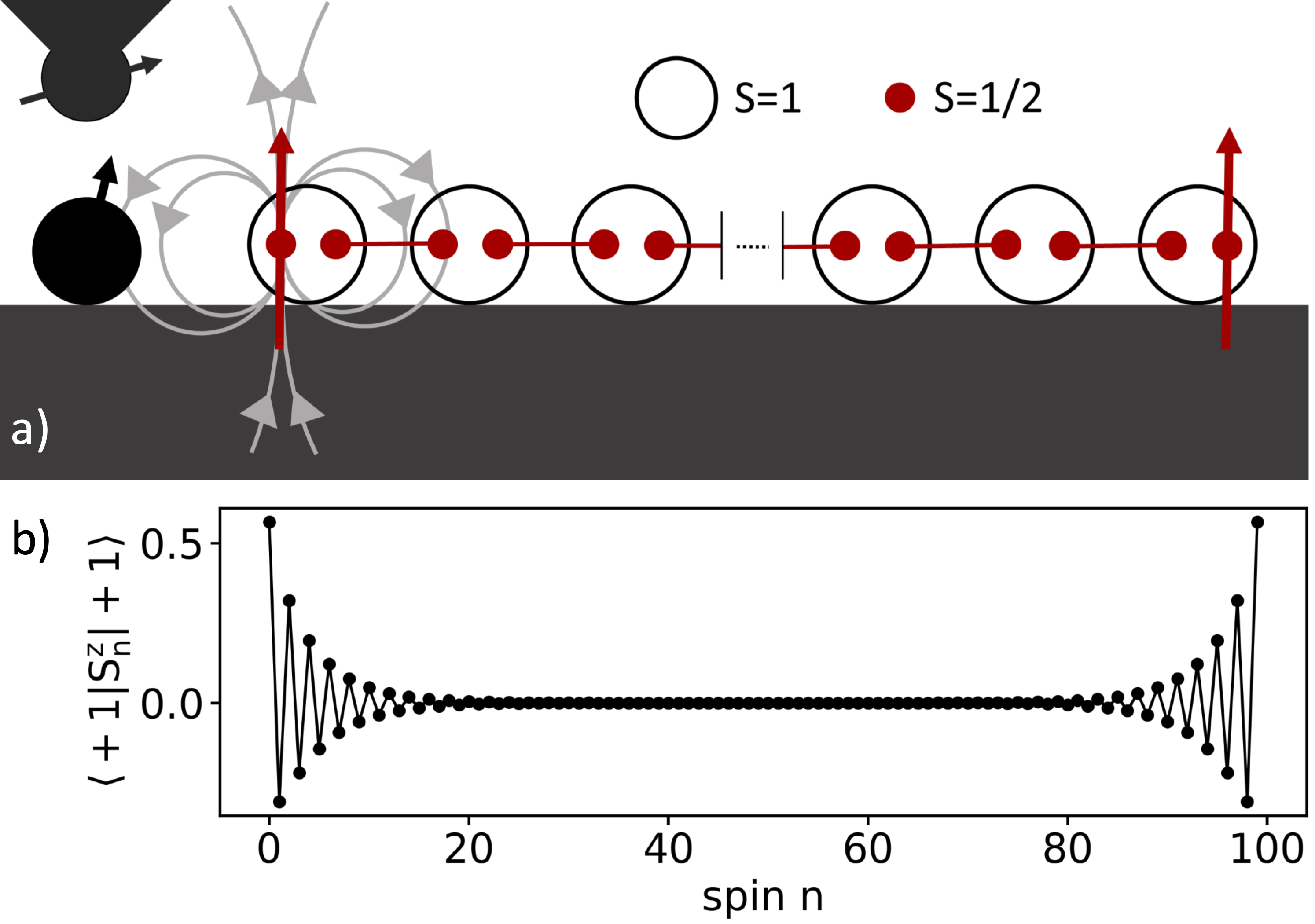
Figure 1: a) Scheme of the proposed experiment to measure fractionalization by means of ESR-STM. A Haldane chain is built on a kondo-free surface. The system is described as if there were two $S=1/2$ objects at the edge. An ESR active atom (sensor atom) is placed near the chain to infer the magnetic moments of such chain from its stray field. b) Spin density of the $S^{z}=+1$ triplet state for $\beta=0.09$.

Our proposal (see Fig. 1) relies on the demonstrated capability of ESR-STM to act as an absolute magnetometer Natterer et al. (2017); Choi et al. (2017). To do so, an ESR-STM active spin acts as a sensor that can be placed at several distances of a second spin or group of spins denoted as target. At finite temperature, the target spins can occupy different quantum states, each of which generates its own stray fieldChoi et al. (2017); del Castillo and Fernández-Rossier (2023). As a result, the ESR-STM spectrum of the sensor spin features several peaks, whose frequency and intensity relate to the stray-field and occupation probability of the quantum state of the target. As we show below, this can be used to obtain a direct measurement of the magnetic moment, and thereby the spin, of the edge states in Haldane spin chains.

We assume that a Haldane spin chain with $N$ spins $S=1$ is placed on a surface and can be described with the Hamiltonian:

$$\begin{split}{\cal H}=\sum_{n=1,N-1}J&\bigg{[}\vec{S}_{n}\cdot\vec{S}_{n+1}+\beta\left(\vec{S}_{n}\cdot\vec{S}_{n+1}\right)^{2}\bigg{]}\\ &+\sum_{n=1,N}g\mu_{B}\vec{S}_{n}\cdot\vec{B}\end{split}$$ (1)

We take values of $\beta$ in the range $0<\beta<\frac{1}{3}$. The low energy manifold is conformed by a singlet with $S=0$ and a $S=1$ triplet. The singlet-triplet splitting is given by the sum of the effective inter-edge coupling and the Zeeman energy:

$$E(S,S^{z})=S\Delta_{ST}(N)+g\mu_{B}S^{z}B^{z},$$ (2)

where $\mu_{B}$ is the Bohr magneton, $g=2$ and $S=0,1$ and $S^{z}=\pm 1,0$. We choose the quantization axis of the spin to be parallel to the external magnetic field.

The singlet-triplet splitting shows an exponential decay given by $\Delta_{ST}\propto e^{-N/\xi}$, where $N$ is the system size and $\xi$ represents the localization length. This quantity remains significantly smaller than the Haldane gap, the energy splitting between the low-energy manifold and the bulk states. The exponential dependence of $\Delta_{ST}$ closely resembles what would be expected if two $S=1/2$ spins were localized at the edges of the chain, with a localization length on the order of $\xi$. This characteristic is illustrated in Fig. 1b, where we calculate the expectation value of the $S^{z}_{n}$ operators for the low-energy states with $S=1$ and $S^{z}=+1$. Clearly, these states form a magnetic texture localized at each edge, with a combined magnetic moment of $S^{z}=\sum_{n=1,N/2}\langle\pm 1|S^{z}_{n}|\pm 1\rangle=\pm 1/2$.

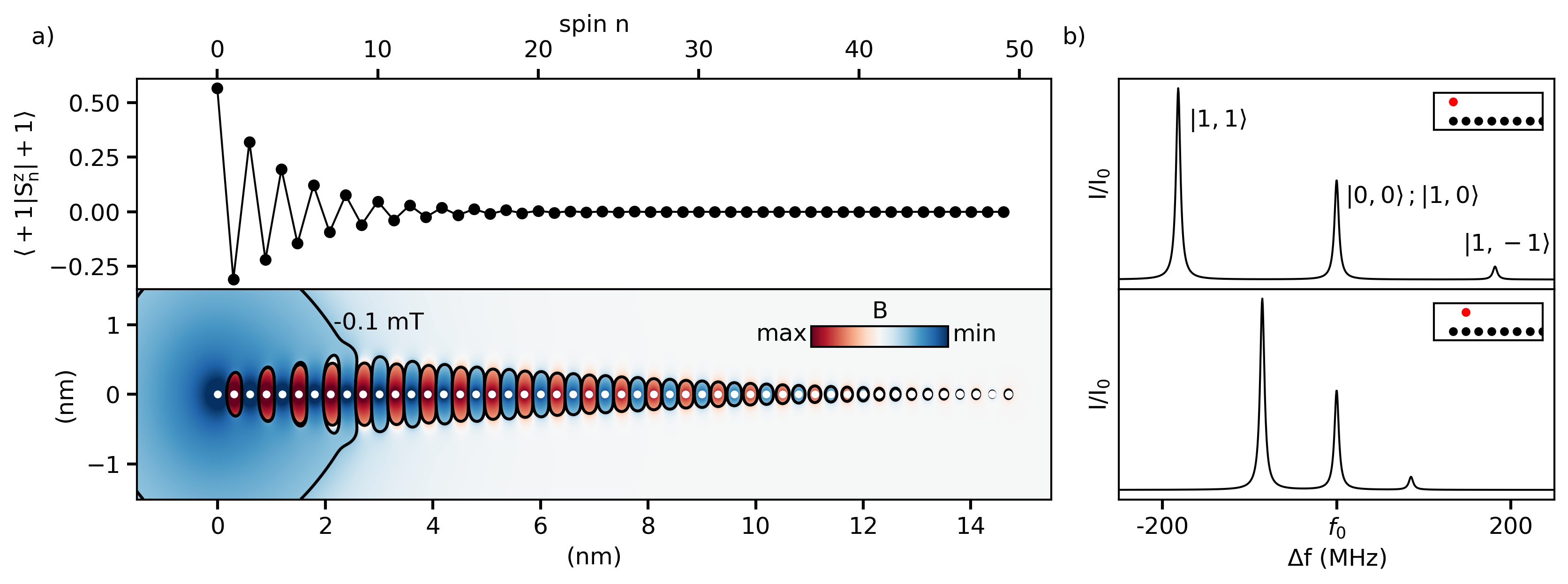
Figure 2: a) The top panel shows the $\langle S^{n}_{z}\rangle$ in the $S^{z}=1$ state of the low-energy manifold for the first half of a Haldane chain of 100 spins with $S=1$ (full chain in the inset). The lower panel illustrates the $z$ component of the stray field generated by the magnetic moments from the spins in the top panel (represented as white dots) on the $xy$ plane. In this example, the chain is located spanning from $(x=0,y=0,z=0)$ to $(x=+Na,y=0,z=0)$. Here, $a$ represents the physical spacing between the $S=1$ spins, treated as point particles. We choose $g=2$ and a spacing of $0.3\text{nm}$ from each other. The contour lines highlight regions where the stray field has a magnitude of $\pm 0.1\text{mT}$. b) ESR spectra produced by the low-energy manifold states of the spin array described in panel a), measured by sensors at different locations (red dots in the inset scheme). The sensors are located at a distance of $0.5\,\text{nm}$ from the array. In this example, $J=18\,\text{meV}$, $T=1\,\text{K}$, $B_{z}=1,\text{T}$, and $\beta=0.09$.

We now consider that an STM-ESR-active spin picks up the straight field generated by a nearby Haldane spin chain. In ESR-STM experiments the DC current across the STM-surface junction is measured as a function of the frequency of the driving voltage. The ESR-STM spectrum for this lateral-sensing setup can be described by the following equation Choi et al. (2017); del Castillo and Fernández-Rossier (2023):

$$I_{DC}(f)=\sum_{\ell}p_{\ell}{\cal L}(f-f(\ell)),$$ (3)

where the sum runs over the eigenstates of the Hamiltonian (eq. 1) of the spin chain, ${\cal H}|\ell\rangle=E_{\ell}|\ell\rangle$, $p_{\ell}=\frac{1}{Z}e^{-E_{\ell}/(k_{B}T)}$ are the thermal occupations of each eigenstate and ${\cal L}(f-f_{\ell})$ is a Lorentzian type resonance curve centered around the frequency $f_{\ell}$. We assume that the external magnetic field is perpendicular to the sample so that the stray field created by the chain at the sensor location is also perpendicular to the substrate. As a result, the resonant frequency of the sensor shifts linearly with the stray field:

$$f(\ell)=\frac{\mu_{B}g_{\rm s}}{h}(B+b(\ell)),$$ (4)

where $h=2\pi\hbar$, and $g_{\rm s}$ is the gyromagnetic factor of the sensor, $B$ and $b_{\ell}$ denote the external field and the stray field generated by the target spins in the state $\ell$, respectively, both along the off-plane direction.

In turn, the stray field is given by:

$$b^{z}(\ell)=-\frac{\mu_{0}}{4\pi}\sum_{n=1}^{N}\frac{m_{n}^{z}(\ell)}{(d^{n})^{3}},$$ (5)

where $d^{n}$ is the distance between the sensor and the spin $n$. The magnetic moment vector $m_{n}^{z}(l)$ is generated by the spin $n$ in each state $\ell$, and its components are given by:

$$m_{n}^{z}(\ell)=-g\mu_{B}\langle\ell|S^{z}_{n}|\ell\rangle.$$ (6)

Equations 3, 4 5, 6 relate the expectation value of the magnetic moments in a given Haldane-chain state $|\ell\rangle$ to the ESR-STM spectrum of a nearby sensor. We now discuss how to determine the magnetic moment of these states and verify fractionalization. Importantly, we assume that the temperature is much smaller than the Haldane gap , so that only the four states of the ground state manifold of the chain contribute to the sum in eq. (3). Only two of these states, with $S=1$ and $S^{z}=\pm 1$ have a non-vanishing expectation value of the spins. The corresponding magnetic profile of the $S^{z}=+1$ states calculated using DMRG White (1992); White and Huse (1993); Catarina and Murta (2023); Lado (2023), is shown in figure 1b, for $\beta=0.09$, relevant for triangulene spin chainsMishra et al. (2021); Henriques and Fernández-Rossier (2023). It corresponds to two physically separated objects with $S^{z}=1/2$ localized at the edges. The $S^{z}=-1$ has analogous properties. In contrast, the expectation value of the spin operators is identically zero when calculated with the $S^{z}=0$ states. Consequently, the four low-energy states of the Haldane spin chain correspond to three distinct magnetic states, with a vanishing stray field for the $S=0$ and $S=1,S^{z}=0$ states, and a finite stray field of opposite sign for the $S^{z}=\pm 1$ states (see Fig. (2a). As a result, the ESR-STM spectrum of the spin-sensor has three distinct peaks corresponding to three different stray fields (See figure 2b). Expectedly, the stray fields of the $S^{z}=\pm 1$ have the same magnitude and opposite sign. From the splitting of these peaks, it is possible to pull out the value of the stray field at the location of the sensor:

$$b^{z}(\pm 1)=\frac{h}{g_{s}\mu_{B}}(f_{0}-f_{\pm 1})$$ (7)

here, $f_{\pm 1}$ represents the resonant frequencies measured at the sensor when the Haldane spin chain occupies the states with $S^{z}=\pm 1$ within the ground state manifold.

In order to determine the magnetic moments of the $N/2$ spins of one half of the chain, that define a vector ${\cal M}\equiv(m_{1}(\pm),...,m_{N/2}(\pm))$, we need to measure the stray field in a set of different locations $N_{M}$, that yields a vector in the readout-location space, ${\cal B}\equiv(b_{1}(\pm),...,b_{N_{M}}(\pm))$. We have considered two methods to pull out the vector ${\cal M}$ out of ${\cal B}$. The first method is the full inversion of the Biot-Savart’s equation (FIBS), that can be written down as ${\cal{B}}=-(\mu_{0}/4\pi)\textbf{D}\cal{M}$, where the elements of the matrix D are $|d^{n}_{n_{m}}|^{-3}$. In this case, it is apparent that the number of necessary readouts equals half of the chain length, $N_{M}=N/2$. The second method involves the use of artificial neural networks and requires a dramatically smaller number of measurements to determine the magnetization map (Fig. 3c,d).

The finite magnetic sensitivity of the readouts, denoted by $\delta{\cal{B}}$ imposes an uncertainty in the determination of the edge magnetic moment. The sensor spectral resolution is ultimately limited by the shot noise sup :

$$\delta B_{\text{min}}=\frac{4}{3}\frac{h\delta f}{g_{s}\mu_{B}}\sqrt{\frac{e}{I_{0}\Delta t}}$$ (8)

where $\delta f$ is the linewidth, $I_{0}$ is the maximal current in the resonance peak, and $\Delta t$ is measurement time, that may be limited by factors such as thermal drift of the tip. The associated minimal shift in the sensor frequency is given by $\Delta f{\rm min}=g\mu_{B}\delta B_{\rm min}/h$ in the range of 1MHz have been reported in STM-ESR magnetometry Choi et al. (2017).

In the case of the FIBS, the uncertainty of the edge magnetic moments is given by:

$$\delta\langle S^{z}\rangle=\left(\frac{4\pi}{\mu_{0}\mu_{B}g}\sum_{n,n_{m}}|(\textbf{D}^{-1})^{n}_{n_{m}}|\right)\delta B_{\rm min}.$$ (9)

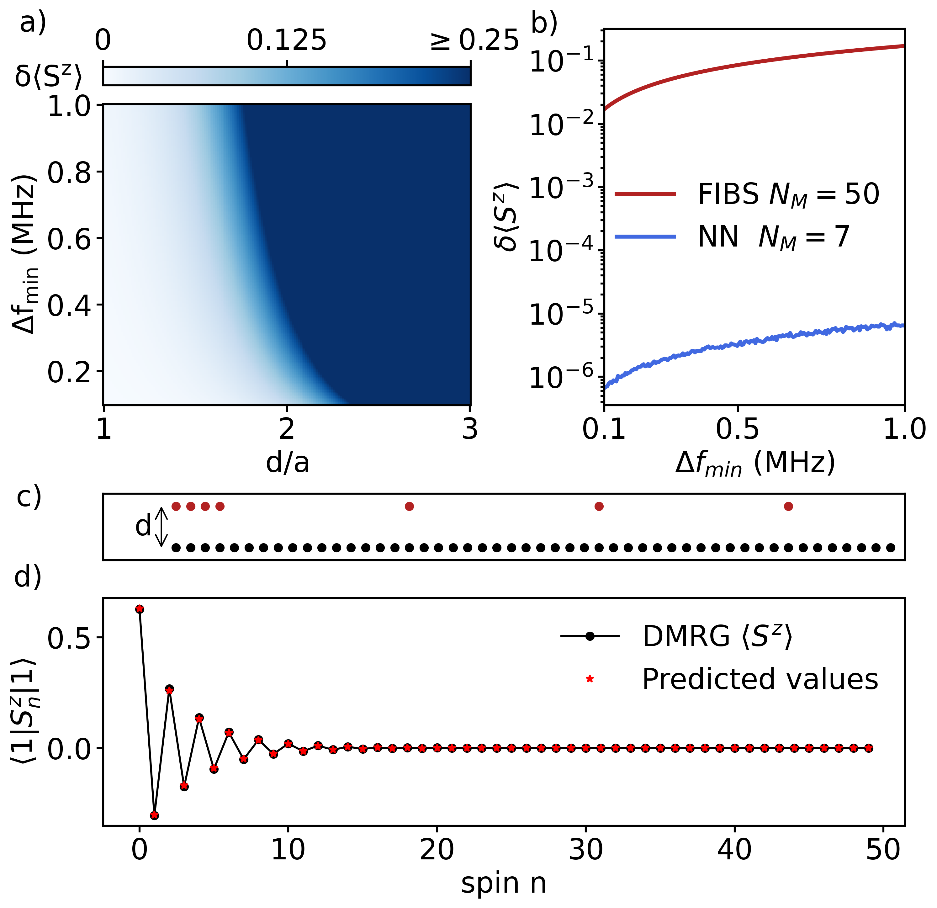
Figure 3: a) $\delta\langle S^{z}\rangle$ as a function of both, the perpendicular distance of the $N_{m}$ sensors to the chain (d) and the spectral resolution $\Delta f_{min}$ for a $S=1/2$ sensor, with $N_{m}=N/2$ different locations from $(x=0,y=d)$ to $(x=+N_{m}a,y=d)$. b) Error comparison between linear inversion of the Biot-Savart’s equation (FIBS) and NN using $N_{m}=7$ sensor positions ($d=0.5$ nm) c) Location of the sensor positions of the NN configuration (red dots) near the spin chain (black dots) d) Neural network prediction of the expectation values of the spins using a magnetic profile with noise compared to the original values

In Figure 3a, we show that assuming the reported resolution, $\Delta f{\rm min}=1\,\text{MHz}$ Choi et al. (2017)), the uncertainty in the determination of the edge spin, $\delta\langle S^{z}\rangle$, is an order of magnitude lower than $\langle S^{z}\rangle$. In principle, longer readout times would make it possible to decrease $\delta f$, and thereby, $\delta\langle S^{z}\rangle$.

We now discuss a second method to invert the Biot-Savart equation that makes use of artificial neuron networks (NN) to invert Biot-Savart’s equation. This method comes with two advantages. First, it reduces the number of ESR-STM measurements. Second, it yields a dramatically smaller uncertainty in the determination of the fractional spin. Our approach involves two different NNs. The first NN classifies magnetic profiles derived from ESR readouts, confirming the presence of the characteristic Haldane spin chain edge magnetization (See Fig. (1b)). The second NN is trained to convert Haldane-type magnetic profiles, with a specific number of measurements, into spin expectation values. The training set incorporates several thousand spin distributions obtained varying $\beta$ between $0$ and $1/3$, each with its characteristic magnetic profile. In addition, we added random noise with amplitude bounded by the magnetic sensitivity range (See Supplemental Material sup ). The synergistic application of these two neural networks reduces the training time to a few minutes on a conventional laptop. This is crucial since a distinct NN needs to be trained for each experimental layout, considering factors such as spin arrangement, sensor positions, sensor type, and spectral resolution.

In Figure 3b, we used $N_{M}=7$ strategically positioned measurements sup , as shown in Figure 3c. Our calculations reveal that, with a number ESR readouts much smaller than $N/2$, it is possible to obtain the magnetization maps and, therefore, the total magnetic moment of half of the chain with an uncertainty as low as $\delta\langle M_{z}\rangle\approx 10^{-4}\mu_{B}$ (See Supplemental Material sup ), as shown in Figure 3b. Consequently, this methodology proves sufficient for determining the presence of an $S=1/2$ object and its localization length, using state-of-the-art ESR-STM instrumentation.

We now discuss how to infer another important property of the edge spins, namely, their localization length $\xi$. This is based on two facts. First, the inversion of the Biot-Savart equation yields the value of the magnetic moment at many sites close to the edge. Second, our numeric work shows that we can parametrize the spins with the following equation:

$$\langle S_{n}^{z}\rangle_{\pm}=\pm(-1)^{n}{\cal A}e^{-\frac{n}{\xi}}$$ (10)

where $\mathcal{A}$ represents the maximum value of $\langle S^{z}_{n}\rangle$ at the edge spin, ensuring that $\sum_{n=1}^{N/2}\langle S^{z}_{n}\rangle=\frac{1}{2}$. Our numerical calculation (see Supplemental Material sup ) shows that the second moment of the magnetization field $\langle n\rangle=\frac{\sum_{n}|\langle S^{z}_{n}\rangle|\cdot n}{\sum_{n}|\langle S^{z}_{n}\rangle|}$ is proportional to $\xi$ in an almost one-to-one relation ($\langle n\rangle\approx 1.02\,\xi$), which permits one to determine this quantity with an uncertainty associated to $\delta\langle S_{n}^{z}\rangle$. For the reported spectral resolution of 1 MHz and d=0.5 nm, the relative errors would be $\frac{\delta\xi}{\xi}\approx 10^{-1}$ for FIBS and $\frac{\delta\xi}{\xi}\approx 10^{-5}$ for NNs sup .

In conclusion, we propose a method to measure the two outstanding properties of the $S=1/2$ fractional degrees of freedom that emerge at the edges of Haldane $S=1$ chains: their fractional magnetic moment $M=g\mu_{B}S$ and their localization length or spatial extension, $\xi$. Our theoretical analysis shows that our method can be implemented with state-of-the-art ESR-STM magnetometry. Our proposal permits one to go beyond previous work, where the presence of fractional degrees of freedom is inferred indirectly, but the actual fractionalization of the magnetic moment is not measured directly. This approach could be used to probe fractional edge spins expected to occur in two-dimensional AKLT models and could also inspire similar experiments using related atomic scale magnetometers, such as NV centers Grinolds et al. (2013); Rondin et al. (2014); Chatterjee et al. (2019); Finco and Jacques (2023).

We acknowledge Arzhang Ardavan for fruitful discussions and Jose Lado for technical assistance on the implementation of DMRG. J.F.R. acknowledges financial support from FCT (Grant No. PTDC/FIS-MAC/2045/2021), SNF Sinergia (Grant Pimag), Generalitat Valenciana funding Prometeo2021/017 and MFA/2022/045, and funding from MICIIN-Spain (Grant No. PID2019-109539GB-C41). YDC acknowledges funding from FCT, QPI, (Grant No.SFRH/BD/151311/2021) and thanks the hospitality of the Departamento de Física Aplicada at the Universidad de Alicante.

References

- Su et al. (1980) W.-P. Su, J. Schrieffer, and A. Heeger, Physical Review B 22, 2099 (1980).
- Tsui et al. (1982) D. C. Tsui, H. L. Stormer, and A. C. Gossard, Physical Review Letters 48, 1559 (1982).
- Laughlin (1983) R. B. Laughlin, Physical Review Letters 50, 1395 (1983).
- Laughlin and Pines (2000) R. B. Laughlin and D. Pines, Proceedings of the national academy of sciences 97, 28 (2000).
- Haldane (1983a) F. Haldane, Physics Letters A 93, 464 (1983a).
- Haldane (1983b) F. D. M. Haldane, Phys. Rev. Lett. 50, 1153 (1983b).
- Affleck et al. (1987) I. Affleck, T. Kennedy, E. H. Lieb, and H. Tasaki, Phys. Rev. Lett. 59, 799 (1987).
- Wei et al. (2011) T.-C. Wei, I. Affleck, and R. Raussendorf, Phys. Rev. Lett. 106, 070501 (2011).
- Saminadayar et al. (1997) L. Saminadayar, D. Glattli, Y. Jin, and B. c.-m. Etienne, Physical Review Letters 79, 2526 (1997).
- De-Picciotto et al. (1998) R. De-Picciotto, M. Reznikov, M. Heiblum, V. Umansky, G. Bunin, and D. Mahalu, Physica B: Condensed Matter 249, 395 (1998).
- Kane and Fisher (1994) C. Kane and M. P. Fisher, Physical review letters 72, 724 (1994).
- Buyers et al. (1986) W. J. L. Buyers, R. M. Morra, R. L. Armstrong, M. J. Hogan, P. Gerlach, Hirakawa, and K., Phys. Rev. Lett. 56, 371 (1986).
- Tun et al. (1990) Z. Tun, W. Buyers, R. Armstrong, K. Hirakawa, and B. Briat, Physical Review B 42, 4677 (1990).
- Yokoo et al. (1995) T. Yokoo, T. Sakaguchi, K. Kakurai, and J. Akimitsu, journal of the physical society of japan 64, 3651 (1995).
- Zaliznyak et al. (2001) I. Zaliznyak, S.-H. Lee, and S. Petrov, Physical Review Letters 87, 017202 (2001).
- Kenzelmann et al. (2003) M. Kenzelmann, G. Xu, I. Zaliznyak, C. Broholm, J. DiTusa, G. Aeppli, T. Ito, K. Oka, and H. Takagi, Physical review letters 90, 087202 (2003).
- Brunel et al. (1992) L. Brunel, T. Brill, I. Zaliznyak, J. Boucher, and J. Renard, Physical review letters 69, 1699 (1992).
- Batista et al. (1999) C. Batista, K. Hallberg, and A. Aligia, Physical Review B 60, R12553 (1999).
- Smirnov et al. (2008) A. Smirnov, V. Glazkov, T. Kashiwagi, S. Kimura, M. Hagiwara, K. Kindo, A. Y. Shapiro, and L. Demianets, Physical Review B 77, 100401 (2008).
- Mishra et al. (2021) S. Mishra, G. Catarina, F. Wu, R. Ortiz, D. Jacob, K. Eimre, J. Ma, C. A. Pignedoli, X. Feng, P. Ruffieux, J. Fernandez-Rossier, and R. Fasel, Nature 598, 287 (2021).
- Delgado et al. (2013) F. Delgado, C. Batista, and J. Fernández-Rossier, Physical Review Letters 111, 167201 (2013).
- Baumann et al. (2015) S. Baumann, W. Paul, T. Choi, C. P. Lutz, A. Ardavan, and A. J. Heinrich, Science 350, 417 (2015).
- Choi et al. (2017) T. Choi, W. Paul, S. Rolf-Pissarczyk, A. J. Macdonald, F. D. Natterer, K. Yang, P. Willke, C. P. Lutz, and A. J. Heinrich, Nature Nanotechnology 12, 420 (2017).
- Yang et al. (2018) K. Yang, P. Willke, Y. Bae, A. Ferrón, J. L. Lado, A. Ardavan, J. Fernández-Rossier, A. J. Heinrich, and C. P. Lutz, Nature nanotechnology 13, 1120 (2018).
- Kovarik et al. (2022) S. Kovarik, R. Robles, R. Schlitz, T. S. Seifert, N. Lorente, P. Gambardella, and S. Stepanow, Nano Letters 22, 4176 (2022).
- Natterer et al. (2017) F. D. Natterer, K. Yang, W. Paul, P. Willke, T. Choi, T. Greber, A. J. Heinrich, and C. P. Lutz, Nature 543, 226 (2017).
- del Castillo and Fernández-Rossier (2023) Y. del Castillo and J. Fernández-Rossier, Phys. Rev. B 108, 115413 (2023).
- White (1992) S. R. White, Physical review letters 69, 2863 (1992).
- White and Huse (1993) S. R. White and D. A. Huse, Phys. Rev. B 48, 3844 (1993).
- Catarina and Murta (2023) G. Catarina and B. Murta, arXiv preprint arXiv:2304.13395 (2023).
- Lado (2023) J. Lado, DMRGpy library (2023).
- Henriques and Fernández-Rossier (2023) J. C. Henriques and J. Fernández-Rossier, Physical Review B 108, 155423 (2023).
- (33) See Supplemental Material for a derivation of equation 8; the details of the NNs approach, the guidelines for sensor positions and its errors; the numerical calculation of the relation between localization length and position operator; and its uncertainties. The Supplemental Material also contains Ref. [34-36].
- Taylor et al. (2008) J. M. Taylor, P. Cappellaro, L. Childress, L. Jiang, D. Budker, P. Hemmer, A. Yacoby, R. Walsworth, and M. Lukin, Nature Physics 4, 810 (2008).
- Dréau et al. (2011) A. Dréau, M. Lesik, L. Rondin, P. Spinicelli, O. Arcizet, J.-F. Roch, and V. Jacques, Physical Review B 84, 195204 (2011).
- Barry et al. (2020) J. F. Barry, J. M. Schloss, E. Bauch, M. J. Turner, C. A. Hart, L. M. Pham, and R. L. Walsworth, Reviews of Modern Physics 92, 015004 (2020).
- Grinolds et al. (2013) M. S. Grinolds, S. Hong, P. Maletinsky, L. Luan, M. D. Lukin, R. L. Walsworth, and A. Yacoby, Nature Physics 9, 215 (2013).
- Rondin et al. (2014) L. Rondin, J.-P. Tetienne, T. Hingant, J.-F. Roch, P. Maletinsky, and V. Jacques, Reports on progress in physics 77, 056503 (2014).
- Chatterjee et al. (2019) S. Chatterjee, J. F. Rodriguez-Nieva, and E. Demler, Physical Review B 99, 104425 (2019).
- Finco and Jacques (2023) A. Finco and V. Jacques, APL Materials 11 (2023).