Variational Autoencoders for Feature Exploration and Malignancy Prediction of Lung Lesions

Abstract

Lung cancer is responsible for 21% of cancer deaths in the UK and five-year survival rates are heavily influenced by the stage the cancer was identified at. Recent studies have demonstrated the capability of AI methods for accurate and early diagnosis of lung cancer from routine scans. However, this evidence has not translated into clinical practice with one barrier being a lack of interpretable models. This study investigates the application Variational Autoencoders (VAEs), a type of generative AI model, to lung cancer lesions. Proposed models were trained on lesions extracted from 3D CT scans in the LIDC-IDRI public dataset. Latent vector representations of 2D slices produced by the VAEs were explored through clustering to justify their quality and used in an MLP classifier model for lung cancer diagnosis, the best model achieved state-of-the-art metrics of AUC 0.98 and 93.1% accuracy. Cluster analysis shows the VAE latent space separates the dataset of malignant and benign lesions based on meaningful feature components including tumour size, shape, patient and malignancy class. We also include a comparative analysis of the standard Gaussian VAE (GVAE) and the more recent Dirichlet VAE (DirVAE), which replaces the prior with a Dirichlet distribution to encourage a more explainable latent space with disentangled feature representation. Finally, we demonstrate the potential for latent space traversals corresponding to clinically meaningful feature changes. Our code is available at https://github.com/benkeel/VAE_lung_lesion_BMVC.

1 Introduction

Lung cancer is the third most common cancer in the UK, accounting for 13% of cases [CR UK (2018)] and the biggest cause of cancer death at 21% [CR UK (2019)]. Early diagnosis of lung cancer is important for prognosis, with five-year survival rates for diagnosis in stages 1–3 at 32.6% compared to 2.9% at stage 4 [ONS (2019)]. Radiologists diagnose lung cancer from medical images including Computed Tomography (CT) scans by visually inspecting lesions in a time-consuming and subjective process [Armato et al. (2009)]. A lesion is an area of tissue which has been damaged and is either a malignant tumour or a benign area of inflammation, abscess or ulcer [Institute (2022)]. CT scans are non-invasive and provide high detail images for medical diagnosis and treatment planning. The main contribution of this research is to:

• Build state-of-the-art prediction models for lung cancer lesions using VAEs.

• Investigate the effectiveness of Dirichlet VAEs for lung lesions, to the best of our knowledge this is the first application in the cancer imaging domain.

Several research papers have investigated the application of AI methods to lung cancer, utilising their ability for complex pattern recognition [Chiu et al. (2022), Jassim and Jaber (2022)]. The Variational Autoencoder (VAE) is an encoder-decoder architecture that maps input data to an $n$-dimensional latent space [Kingma and Welling (2013)]. Smoothness constraints on the latent space, typically enforced using a Gaussian distribution, promote clustering between similar images. Assuming this space captures sufficient information, these latent vectors can be used for classification purposes. Exploration of the space via latent arithmetic and clustering can lead to new insights about a dataset [Higgins et al. (2017), Klys et al. (2018), Shon et al. (2022)].

This paper also explores the use of a Dirichlet distribution in place of the Gaussian. The $K$-dimensional Dirichlet distribution is a multivariate generalisation of the beta distribution with $K$ strictly positive parameters, $\left\{\alpha_{i}\in\mathbb{R}^{+}\right\}^{i=K}_{i=1}$. These $\alpha$ parameters influence the sparsity and density of the probability simplex, the impact of different values is shown in Figure 1. The sum of the $\alpha$ values is known as the concentration parameter, which controls the dispersion. When all $\alpha$ equal $1$ it is a uniform distribution (Figure 1 (b)) and a lower/higher sum causes sparsity/density (Figure 1 (a), (c), (d)). A relatively high $\alpha_{i}$ will encourage more probability to be concentrated in the corresponding area of the simplex (Figure 1 (e), (f)). Choosing target $\alpha$ values in DirVAE influences the distribution of the VAE latent space.

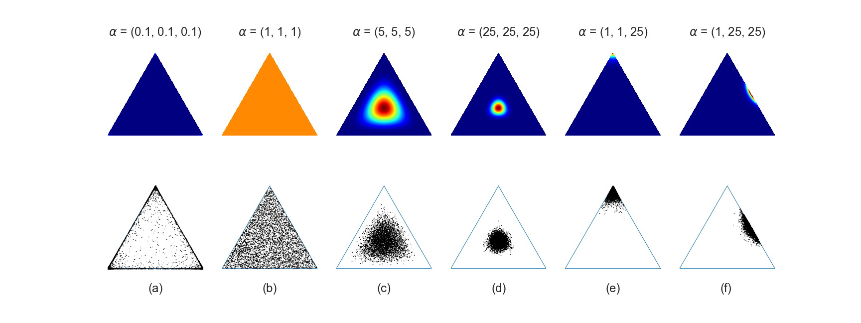
Figure 1: Examples of Dirichlet distribution simplex with 5000 samples given $\alpha$ parameters.

In summary, VAE models will be trained on 2D slices of CT scans cropped to lung lesions. The latent vector representations are used in Multilayered Perceptron (MLP) classification models for the task of lung cancer diagnosis. The latent vectors will be evaluated to justify their quality as feature vectors by showing that tumours with similar characteristics are grouped together in the latent space and to demonstrate the ability to predictably change features. This enhances the explainability of the method as it is more intuitive and interpretable for a non-technical audience. Additionally, comparisons between the Gaussian and Dirichlet latent space will show that the DirVAE has better disentanglement of features. To inform this research, we conducted a review of the published literature on AI for lung lesion diagnosis, applications of VAEs in the cancer domain and applications of DirVAEs.

2 Related Works

Jassim and Jaber (2022) conducted a systematic review of Artificial Intelligence (AI) for lung lesion diagnosis from medical images in the years 2017-2021 and found an accuracy range of 88% to 99.2% and AUC range of 0.7 to 0.967. Over half of the studies use 2D Convolutional Neural Network (CNN) architectures for feature extraction and a separate classifier, with transfer learning (TL) commonly applied. For instance, Mathews and Jeyakumar (2020) used TL with ResNet 50 He et al. (2015) and a shallow CNN, achieving 97.6% accuracy. Additionally, some studies have fused clinically known features with CNN derived features, for instance, Xie et al. (2018) obtained AUC of 0.967 and an accuracy of 89.5%. Jassim and Jaber (2022) did not include any papers applying VAE to lung cancer detection, however, there are some existing studies in this domain Silva et al. (2020); Astaraki et al. (2021); Gao et al. (2023). In the most similar study with the best diagnostic performance using VAEs, Silva et al. (2020) applied a VAE to lesions extracted from the LIDC-IDRI dataset and used retraining of the encoder with a Multi-Layered Perceptron (MLP) classifier, achieving AUC of 0.936. Additionally, several papers have applied VAEs to lung cancer for other tasks including segmentation, survival analysis and tumour growth prediction Pastor-Serrano et al. (2021); Li et al. (2022); Vo et al. (2020); Xiao et al. (2020); Jiang et al. (2021); Wang and Wang (2019). This paper builds upon the work of Silva et al. (2020) by improving both the diagnostic performance and the interpretability of the method.

Regarding the application of generative models to the cancer domain, several papers have explored the value of VAEs for latent space exploration Wang and Wang (2019); Schön et al. (2022); Kleesiek et al. (2021). For instance, Wang and Wang (2019) used VAEs to learn latent representations of the DNA to classify lung cancer subtypes. Kleesiek et al. (2021) used an approach based on autoencoders and GANs for generating synthetic abdominal CT scans and demonstrated adding and removing liver lesions.

Several previous studies have proposed VAEs which replace the prior distribution with a Dirichlet. However, to our knowledge, our work is the first to apply this idea within a cancer setting. The DirVAE was originally proposed by Srivastava and Sutton (2017) and was subsequently utilised in similar studies on topic modelling by Xiao et al. (2018) and Burkhardt and Kramer (2019). Later studies applied the model to image classification and demonstrated that DirVAE latent vectors were very capable in clustering images from the same category and separating them from others Joo et al. (2020); Gawlikowski et al. (2022). Li et al. (2020) proposed an approach which combined graph neural networks and the DirVAE for abstract graph clustering. In the medical domain, Kshirsagar et al. (2022) used the approach to disentangle DNA sequences into different cell types. Most recently, Harkness et al. (2023) used the DirVAE for chest X-ray classification.

Using the Dirichlet distribution in a VAE requires a reparameterisation trick which can produce a differentiable sample from the theoretical distribution. Various techniques have been used before which include the Laplace approximation Li et al. (2020), approximation of the inverse CDF Joo et al. (2020), rejection sampling variational inference Burkhardt and Kramer (2019) and implicit reparamterisation gradients Figurnov et al. (2018). Instead, sampling from the Dirichlet distribution is done using the pathwise gradient method introduced in Jankowiak and Obermeyer (2018) and subsequently implemented in PyTorch.

3 Methods

3.1 Dataset and Pre-Processing

The LIDC-IDRI public dataset contains 1,010 CT scans, consisting of 20,801 2D image slices which range from 0.6 to 5.0 mm thick with expert annotations Armato et al. (2011, 2015). The dataset was then limited to 875 patients with a lesion present totalling 13,916 slices. Silva et al. (2020) reported that the LIDC-IDRI contains 2,669 lesions larger than 3 mm. The lesions are categorised as malignant, ambiguous or benign in 5,249, 5,393 and 3,274 slices respectively, corresponding to 394, 580 and 454 patients. Note that some patients exhibit all three types. These labels were assigned based on a score of 1-5 agreed by four experienced thoracic radiologists: lesions with a score of 1 or 2 are benign, 3 is ambiguous, and 4 or 5 are malignant. All slices have segmentation masks that indicate where the lesion is located. Lesions measuring less than 3 mm in diameter and additionally any with less than 8 pixels were removed as they correspond to much smaller lesions which are not clinically relevant Gould et al. (2013); Xu et al. (2006).

Image slices are 512x512 pixels covering the cross-section of the body, from this a region of interest (ROI) of size 64x64 containing the segmentation masks was selected. Subsequently, 24 slices were excluded as they did not fit in the ROI and a further 64 slices as the bounding box went over the edge of the image, leaving a total of 13,852 in the final dataset.

Pixels in the scan are dimensionless Hounsfield units (HUs) in the range$[-3000,3000]\in\mathbb{R}$. HUs measure the intensity of an X-ray beam, which is altered based on the density of a structure. In this context, HU values below -1000 correspond to air, above 400 are bone, and in between are tissues. Since this work is concerned with lesions which are based in the tissues, upper and lower limits are set for the HU and values are scaled to the range $(0,1)$ as in Silva et al. (2020). This scaling will help to homogenise structures of bone and air to reduce variation.

3.2 Model Description and Training

3.2.1 Initial VAE Training

The VAE architecture proposed in this paper is visualised in Figure 2. The architecture is loosely adapted from Hansen (2019) with additional hyperparameter training and different activation functions. The encoder component uses blocks of 2D Convolutional (Conv) layers with a Gaussian Error Linear Unit (GELU) activation function Hendrycks and Gimpel (2016) and 2D Batch Normalisation Ioffe and Szegedy (2015). For the Gaussian VAE, the output of the encoder is used in two separate 2D Conv layers for mean ($\mu$) and log variance $\left(\text{log}(\sigma^{2})\right)$, whereas in the DirVAE a single 2D linear layer is used for the alpha ($\alpha$) parameters. These layers form a latent space of lesion feature representations for the respective models. The decoder takes a parameterised version of the latent vectors, sampled from an $n$-dimensional Gaussian or Dirichlet distribution. The decoder is a symmetric architecture which applies upsampling to the feature maps to reconstruct the images. Firstly, with a 2D Convolutional Transpose layer and secondly, using a combination of bilinear interpolation with 2D Conv layers. This second approach is less computationally expensive and helps avoid artifacts Odena et al. (2016). The decoder produces a tensor of the same shape as the input containing the reconstructed images which are then evaluated against the original images in the loss function.

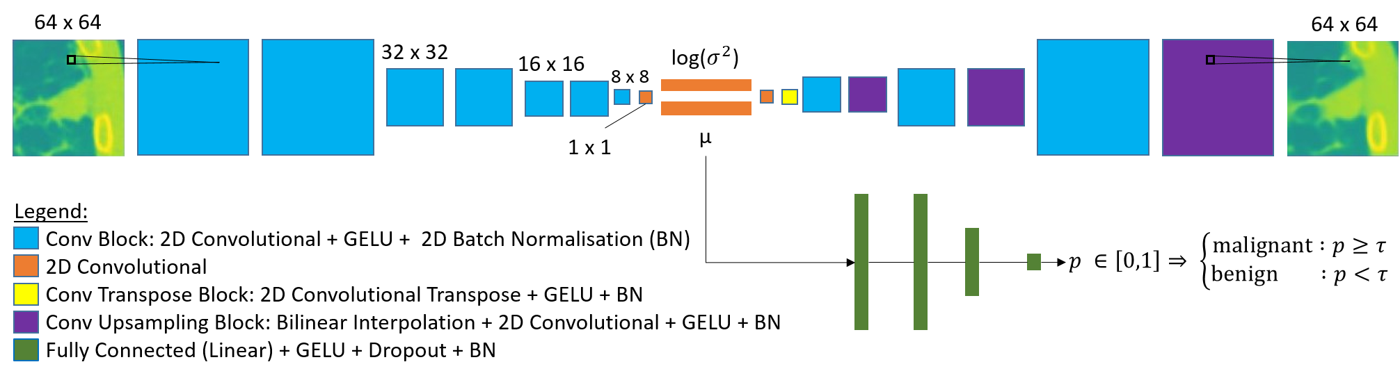
Figure 2: Proposed Model Architecture: VAE with MLP classifier. The feature map size is in the format ‘$n$ x $n$’ and these sizes follow left to right. The decoder architecture is symmetric to the encoder. Note that the final layers for the VAE and MLP have Sigmoid activation instead of GELU and do not have Batch Normalisation (BN) or Dropout.

The loss function is a weighted combination of three terms: the L1 Loss, the Kullback-Leibler Divergence (KLD) Kullback and Leibler (1951) and the Structural Similarity Index Measure (SSIM) Wang et al. (2004) or the Multi-Scale SSIM (MS-SSIM) Wang et al. (2003) for each image $i$ as follows,

$$\frac{1}{\text{batch\_size}\cdot\text{base}}\displaystyle\sum_{i=1}^{n}\lambda\cdot\psi\cdot\text{L1 Loss}_{i}+(1-\lambda)\cdot\gamma\cdot\text{SSIM}_{i}+a\cdot\beta_{\text{norm}}\cdot\text{KLD}_{i}.$$ (1)

The scale factor ${(\text{batch\_size}\cdot\text{base})}^{-1}$ is applied so that the values are consistent across different hyperparameters; ‘base’ is a scalar parameter controlling the number of feature maps in the VAE model. The first two components, L1 Loss and either SSIM or MS-SSIM, measure image reconstruction quality and the KLD is the standard measure of latent space smoothness Kingma and Welling (2013). The reconstruction metrics are balanced using the hyperparameter constant $\lambda\in[0,1]$. Two other hyperparameters are used to weight theses components, $\psi\in\{1,2,3\}$ and $\gamma\in\{0,1,\text{batch\_size}\}$ which is used to either exclude or include the mean or the sum of the SSIM. Finally, the KLD is scaled by the hyperparameter $\beta_{\text{norm}}=\beta\cdot\frac{\text{latent\_size}}{\text{image\_size}}$, as discussed in Higgins et al. (2017), this formulation with $\beta>1$ leads to better disentanglement of the latent space, here $\beta$ values are in the range $[1,50]$. An annealing function $a$ was also included which linearly decreases the KLD by a maximum of 1 across the training epochs. The loss function was altered based on the above hyperparameters to find a combination which balanced the adversarial objectives of image quality and latent space smoothness.

In total, the VAE models have 12 trainable hyperparameters which were explored using a random search strategy, including upper and lower bound for the HU, number of feature maps in VAE layers (base), size of the latent vector, the 4 parameters in the loss function in equation 1, whether to use the SSIM or MS-SSIM, whether or not annealing was applied to the KLD, the learning rate and batch size. The DirVAE had an additional hyperparameter for the target alpha parameters which the KLD compares against tries to move towards. The values are in the range $\alpha_{i}\in[0.5,0.99]$, ranging from a sparse and disentangled distribution to almost a uniform distribution at higher values (c.f. Figure 1 (a) and (b)).

The dataset of 875 patients was randomly split 70/30 into train and test sets with approximately 613 and 262 patients. The VAE reconstructions were evaluated qualitatively, and quantitatively with the average SSIM, Mean Squared Error (MSE) and Mean Absolute Error (MAE) which are conventionally used in the literature.

3.2.2 Fine-Tuning and Classification

After initial training, the loss function (1) is updated to add a new term ‘$\text{BCE}_{i}$’ which is the binary cross entropy loss Bridle (1991) of the MLP malignancy classifier Haykin (1994) shown in the model architecture (Figure 2). The aim is to enable the VAE to be simultaneously useful for reconstruction and classification.

We employ a greedy optimisation strategy similar to Expectation-Maximimisation (EM) optimisation as described in the following pseudocode.

1. Train the VAE model using loss function (1) and extract the latent vectors.

2. Using these latent vectors, find optimal hyperparameters for the MLP classifier using BCE loss.

3. Repeat steps 1 and 2 until convergence, adding the BCE loss of the current optimal MLP to the loss function.

The MLP hidden layers include GELU activation, dropout and batch normalisation, with a sigmoid activation on the output layer to return probabilities, with a parameter $\tau$ controlling the threshold beyond which a example is predicted as positive. The key hyperparameters which were trained using a random search strategy include $\tau$ with a value in the range $[0.4,0.6]$, learning rate, batch size, number of nodes in each layer, whether there are 4 or 5 layers and a dropout probability. The 13,852 slices were split into 5 sets with train, validation and test sets in ratio $3:1:1$ for 5-fold cross-validation; evaluation metrics are reported as the mean of these runs with standard deviations given for AUC and accuracy. Classification performance will be evaluated using the AUC primarily, though we also report the accuracy, precision, recall, specificity, and F1-score. The VAE and MLP models were built in Python 3.9 using PyTorch 1.12 and trained using the Adam optimiser Kingma and Ba (2014).

3.2.3 Clustering and Latent Space Exploration

Two clustering methods, K-Means MacQueen (1967) and CLASSIX Chen and Güttel (2022), were used to partition the latent vectors into distinct groups. An optimal range of values for parameter $k$, the number of clusters in K-Means, was investigated with an elbow graph of the sum of squared distances within each cluster to find a good balance in the number of clusters and their density. The density parameter in CLASSIX is chosen using a grid search to maximise separation by malignancy class. K-Means is non-deterministic and so results are averaged over 50 runs.

Directions in the latent space corresponding to feature changes were found by collecting two groups of latent vectors, with and without a desired feature and taking the average direction vector between the groups. Latent traversal figures were produced by applying multiples of the direction vector to a new image and plotting the decoded images.

4 Results

4.1 VAE Lung Lesion Reconstructions

Here a random sample of 16 images and the reconstructions by the GVAE are qualitatively reviewed in Figure 3. Firstly, observe that the overall macrostructure is captured well and so are most of the microstructures, however, some heterogeneity is lost. The most obvious missing information is that some of the lung parenchyma which could be alveoli are not fully captured in the reconstructed versions. Clinical collaborators specialising in oncology, AQ and DJ, confirmed the reconstructions captured the important clinical features considered in diagnosis. Based on a hyperparameter search of around 120 GVAE and 40 DirVAE candidates, overall the DirVAE had a poorer image reconstruction. The best GVAE achieved SSIM of 0.89, MSE of 0.0032 and MAE of 0.027, whereas the best DirVAE achieved SSIM 0.65, MSE of 0.017 and MAE of 0.055.

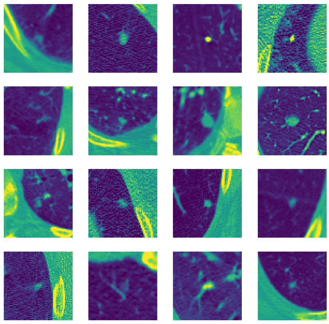
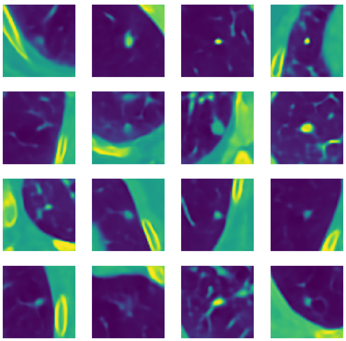
Figure 3: Demonstration of VAE reconstruction quality with original images (a) and the corresponding VAE reconstructions (b).

4.2 Classification Performance

Results are generated from a mean of 5-fold cross-validation of MLP classifiers and are summarised in Table 1. Separate results are given for 1: malignant vs non-malignant and 2: malignancy vs benign with ambiguous excluded. This method achieves state-of-the-art results exceeding the maximum AUC of 0.967 from Jassim and Jaber (2022) (c.f. Section 2). For a direct comparison with similar methodology, Silva et al. (2020) achieved AUC 0.936 after retraining the encoder. For a comparison to clinical radiologist performance, Al Mohammad et al. (2019) conducted a study based on 60 CT scans evaluated by 4 expert radiologists and compared to pathologically confirmed cases. The radiologists had a mean AUC of 0.846, recall of 0.749, specificity of 0.81. Results provided give performance metrics after initial training and after Expectation-Maximisation optimisation with the classifier loss (‘$X_{EM}$’). Clearly, the fine-tuning improves the performance of the classifiers but also the VAE performance metrics for image reconstruction and the KLD do not significantly change and in most cases improve. The best individual model performance outside of cross-validation is a malignant vs benign classifier using GVAE latent vectors which achieved AUC 0.99 and 95.9% accuracy. Overall the EM-optimised VAEs had a virtually idenitcal performance, the GVAE had the highest AUC of 0.98 and DirVAE had the highest accuracy of 93.9%.

Table 1: Latent vector malignancy classifier results before and after Expectation Maximisation (EM) optimisation. 1: malignant vs non-malignant, 2: malignant vs benign for Gaussian (G) and Dirichlet (D) variants. Results given as $\mu\pm\sigma$ (mean $\pm$ std dev) across 5 runs.

Model	AUC	Accuracy	Precision	Recall	Specificity	F1 Score
$G1_{EM}$	0.975 $\pm 0.004$	0.934 $\pm 0.014$	0.90	0.92	0.94	0.91
$D1_{EM}$	0.974 $\pm 0.001$	0.933 $\pm 0.001$	0.90	0.92	0.94	0.91
$G1$	0.850 $\pm 0.017$	0.793 $\pm 0.018$	0.69	0.74	0.82	0.71
$D1$	0.831 $\pm 0.020$	0.782 $\pm 0.030$	0.65	0.74	0.80	0.69
$G2_{EM}$	0.980 $\pm 0.008$	0.931 $\pm 0.017$	0.93	0.96	0.89	0.94
$D2_{EM}$	0.978 $\pm 0.007$	0.939 $\pm 0.020$	0.93	0.96	0.90	0.95
$G2$	0.894 $\pm 0.021$	0.819 $\pm 0.027$	0.81	0.88	0.74	0.84
$D2$	0.841 $\pm 0.013$	0.770 $\pm 0.017$	0.81	0.81	0.70	0.81

4.3 Clustering and Latent Space Exploration

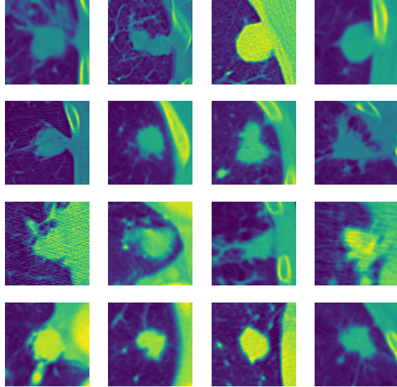
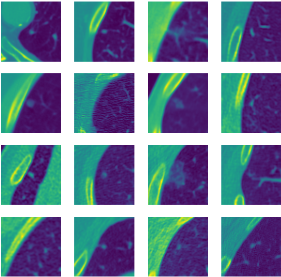
Figure 4: Latent vectors clustered by visual features: sample of 16 images from a cluster with 100% malignant lesions (a) and a cluster with 97% non-malignant lesions (b).

In Figure 4 visual similarities can be observed, for instance in (a) there is a large circular mass in the centre, whereas in (b) more bone is concentrated in the top left corner.

Table 2: CLASSIX (C) and K-Means (KM) clustering statistics. Patient abbreviated as Pt.

Statistic	$G_{C}$	$D_{C}$	$G_{KM}$	$D_{KM}$
Pt in a single cluster	13%	25%	15%	19%
50% Pt slices in one cluster	33%	51%	35%	42%
25% Pt slices in one cluster	81%	91%	80%	84%
Clusters with above 75% of one class	66%	77%	75%	63%
Clusters with above 66.67% of one class	82%	88%	86%	78%

Clustering statistics for the GVAE (G) and DirVAE (D) models with 131 clusters are given in Table 2; these show that the latent space is capable of separating the lesions based on clinically relevant features such as tumour size and malignancy class, and furthermore attempts to group multiple images of the same patient together. It is worth noting that this clustering is post EM optimisation, which increased the separation by malignancy class. This indicates that the VAE was encouraged to encode features related to class in the latent space. Although, the clusters already had a high separation before using the classifier loss which indicates the latent space naturally encodes these meaningful attributes.



Finally, to demonstrate the capabilities of VAE models in this domain, in Figure 5 there are two examples of latent space traversals (c.f. Section 3.2.3). These directions were applied to a new lesion not used in finding the direction and it appears to generalise well including maintaining the surrounding bone structure and generating realistic images at each step. Animations of latent traversals were generated by this analysis showing smooth transitions with more samples. Traversals are constructed by sampling from the latent space, either by using a start and end image and interpolating, or choosing a start point and moving in the direction of the desired feature as in Figure 5. Note that all images other than the start point are synthetic. Further examples are provided on the GitHub page.

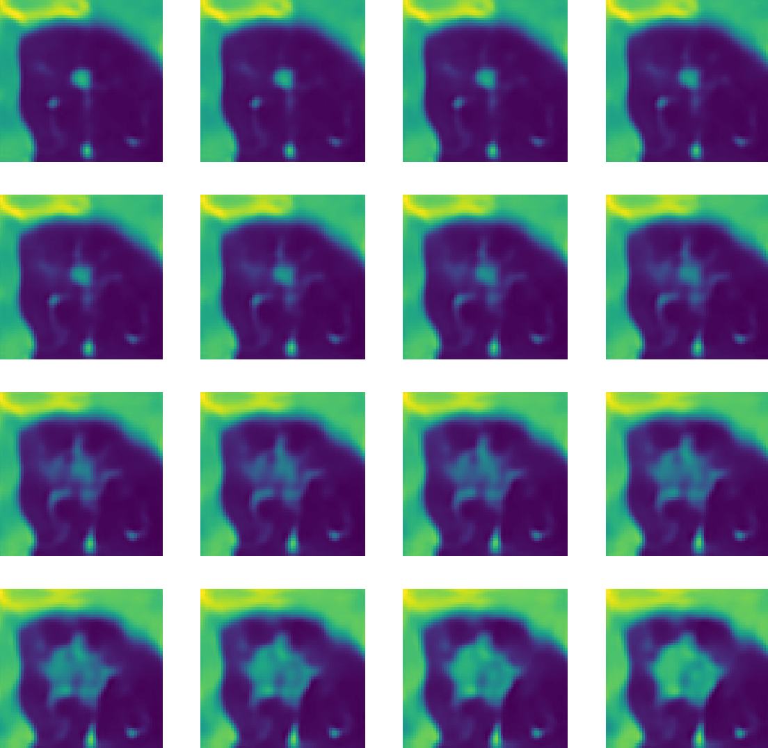
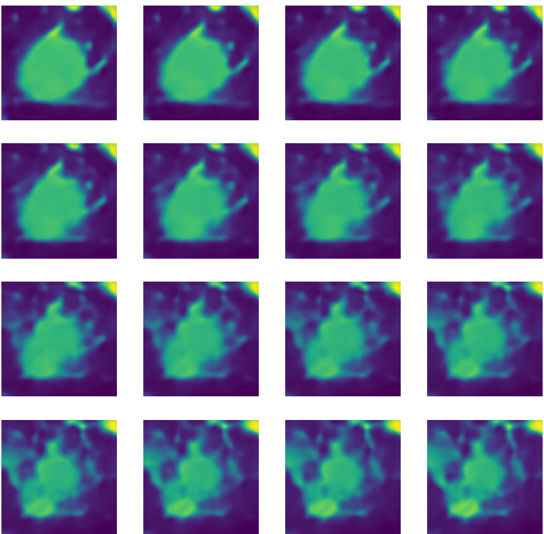
Figure 5: Capability for clinically meaningful traversals in the latent space related to lung tumour growth (a) and increased parenchyma/irregular tumour border (b) (c.f. Section 3.2.3).

5 Discussion

The most significant contribution of this work is the novel use of DirVAEs in the cancer imaging domain. This work has also shown that a VAE and MLP combination can achieve state-of-the-art classification performance for lung lesion diagnosis with AUC 0.98 which compares to radiologist performance of 0.846 and is on par with the best AI-based approaches. Overall the results suggest that both approaches produce good classification models, the key difference is that the DirVAE demonstrates greater disentanglement and separation by clinically meaningful characteristics, whilst GVAE produces better reconstructions. In practice, the best model will likely depend upon the context, dataset and specific task.

This approach for encoding the images with a VAE lends robustness and an element of explainability as we can observe that lesions with similar characteristics have representations that are close together in the latent space as demonstrated by the clustering results. This aspect of the work may be valuable for generating pseudo-labels in tasks without a ground truth. Although this paper demonstrates accurate classification models, it is important to discuss some of the limitations of the proposed method. Firstly, the labels are generated by expert radiologists rather than the gold standard of pathological confirmation. Secondly, the data uses a non-standardised slice thickness, while some may argue it is better to standardise, this approach may be more generalisable to the real world. One further limitation of the 2D approach is that slices from the same patient are not independent both in structure and the likelihood of malignancy. While extending this analysis to 3D may produce a more robust model, data samples would reduce from 13,852 to 875 and model complexity would increase.

Some of the lung parenchyma were not fully captured by the latent vectors as demonstrated in Figure 3. However, the lung naturally has more connective tissue septa than other parts of the body and these hold little relevance to malignancy diagnosis, meaning that failure to capture the parenchyma could actually increase the signal-to-noise ratio. Further experimentation is needed to determine whether they are important for the overall classification.

6 Conclusion and Future Work

Overall, (1) VAEs with Gaussian and Dirichlet priors were trained to produce a latent space which was capable of capturing macro details to a very high standard and micro details to a satisfactory standard. (2) Clustering algorithms were implemented, with results showing that latent vectors were clustered by patient and lesion type and that the Dirichlet prior was better at separating the data in this way. (3) MLP classifiers for malignant or benign lesions were trained using latent vectors from the VAEs, the best model achieved state-of-the-art performance with an AUC of 0.98 and 93.1% accuracy.

Future work could include combining 2D slice level prediction into higher level predictions such as at the 3D lesion or patient level. This would mitigate the limitations associated with a 2D approach including slice thickness and independence of samples. Further improvements to the VAE methodology could include segmenting bone and fat to remove this impact from the latent space. Additionally, extending the latent space exploration to see how different features affect classifications. For instance, using the tumour growth direction or other feature changes such as adding/removing parenchyma to see the impact on the probability of malignancy. Applying methods for latent direction discovery by selecting the best traversals based on metrics such as largest change in prediction score. Finally, to look at implementing DirVAE latent traversals along single dimensions to demonstrate its disentanglement and to add value for model interpretation.

References

- Al Mohammad et al. (2019) B. Al Mohammad, S. L. Hillis, W. Reed, M. Alakhras, and P. C. Brennan. Radiologist performance in the detection of lung cancer using CT. Clinical Radiology, 74(1):67–75, 2019. URL https://doi.org/10.1016/j.crad.2018.10.008.
- Armato et al. (2009) Samuel G Armato, Rachael Y Roberts, Masha Kocherginsky, Denise R Aberle, and Ella A Kazerooni et al. Assessment of Radiologist Performance in the Detection of Lung Nodules : Dependence on the Definition of "Truth". Academic Radiology, 16(1):28–38, 2009. URL https://pubmed.ncbi.nlm.nih.gov/19064209/.
- Armato et al. (2011) Samuel G. Armato, Geoffrey McLennan, Luc Bidaut, Michael F. McNitt-Gray, and Charles R. Meyer et al. The lung image database consortium (lidc) and image database resource initiative (idri: A completed reference database of lung nodules on ct scans. Medical Physics, 38(2):915–931, 2011. URL https://doi.org/10.1118/1.3528204.
- Armato et al. (2015) Samuel G. Armato, Geoffrey McLennan, Luc Bidaut, Michael F. McNitt-Gray, and Charles R. Meyer et al. Data from lidc-idri. the cancer imaging archive. 2015. URL https://doi.org/10.7937/K9/TCIA.2015.LO9QL9SX.
- Astaraki et al. (2021) Mehdi Astaraki, Yousuf Zakko, Iuliana Toma Dasu, Örjan Smedby, and Chunliang Wang. Benign-malignant pulmonary nodule classification in low-dose CT with convolutional features. Physica Medica, 83(March):146–153, 2021. ISSN 1724191X. URL https://doi.org/10.1016/j.ejmp.2021.03.013.
- Bridle (1991) John S Bridle. Probabilistic interpretation of feedforward classification network outputs, with relationships to statistical pattern recognition. Proceedings of the Royal Society of London. Series B, Biological Sciences, 244(1310):175–196, 1991. URL https://link.springer.com/chapter/10.1007/978-3-642-76153-9_28.
- Burkhardt and Kramer (2019) Sophie Burkhardt and Stefan Kramer. Decoupling sparsity and smoothness in the dirichlet variational autoencoder topic model. Journal of Machine Learning Research, 20:1–27, 2019. URL https://jmlr.org/papers/v20/18-569.html.
- Chen and Güttel (2022) Xinye Chen and Stefan Güttel. Fast and explainable clustering based on sorting. arXiv EPrint arXiv:2202.01456, The University of Manchester, UK, 2022. URL https://arxiv.org/abs/2202.01456.
- Chiu et al. (2022) Hwa-Yen Chiu, Heng-Sheng Chao, and Yuh-Min Chen. Application of artificial intelligence in lung cancer. Cancers, 14(6), 2022. ISSN 2072-6694. 10.3390/cancers14061370. URL https://www.mdpi.com/2072-6694/14/6/1370.
- CR UK (2018) CR UK. Cancer incidence for common cancers, cancer research uk. https://www.cancerresearchuk.org/health-professional/cancer-statistics/incidence/common-cancers-compared#heading-Zero, 2018.
- CR UK (2019) CR UK. Cancer mortality for common cancers, cancer research uk. https://www.cancerresearchuk.org/health-professional/cancer-statistics/mortality/common-cancers-compared#heading-Zero, 2019.
- Figurnov et al. (2018) Michael Figurnov, Shakir Mohamed, and Andriy Mnih. Implicit reparameterization gradients. Advances in Neural Information Processing Systems, 2018-December(NeurIPS):441–452, 2018. URL https://dl.acm.org/doi/10.5555/3326943.3326984.
- Gao et al. (2023) Zhihui Gao, Ryohei Nakayama, Akiyoshi Hizukuri, Kosuke Shibuya, and Shoji Kido. Anomaly Detection for Lung CT Images Using SVDD-AE. pages 734–735, 2023. URL https://doi.org/10.1109/gcce56475.2022.10014074.
- Gawlikowski et al. (2022) Jakob Gawlikowski, Sudipan Saha, Anna Kruspe, and Xiao Xiang Zhu. An Advanced Dirichlet Prior Network for Out-of-Distribution Detection in Remote Sensing. IEEE Transactions on Geoscience and Remote Sensing, 60:1–19, 2022. URL https://doi.org/10.1109/TGRS.2022.3140324.
- Gould et al. (2013) Michael K. Gould, Jessica Donington, William R. Lynch, Peter J. Mazzone, and David E. Midthun et al. Evaluation of individuals with pulmonary nodules: When is it lung cancer? Chest, 5(143), 2013. URL https://doi.org/10.1378/chest.12-2351.
- Hansen (2019) L. Hansen. Mec19 vae tutorial solution, github. https://github.com/multimodallearning/mec19_vae_tutorial_solution/blob/master/colab/mec19_vae_tutorial_solution.ipynb, 2019.
- Harkness et al. (2023) Rachael Harkness, Alejandro F Frangi, Kieran Zucker, and Nishant Ravikumar. Learning disentangled representations for explainable chest X-ray classification using Dirichlet VAEs. 2023. URL http://arxiv.org/abs/2302.02979.
- Haykin (1994) Simon Haykin. Neural networks: a comprehensive foundation. Prentice Hall PTR, 1994.
- He et al. (2015) Kaiming He, Xiangyu Zhang, Shaoqing Ren, and Jian Sun. Deep residual learning for image recognition. CoRR, 2015. URL http://arxiv.org/abs/1512.03385.
- Hendrycks and Gimpel (2016) Dan Hendrycks and Kevin Gimpel. Gaussian error linear units (gelu). 2016. 10.48550/ARXIV.1606.08415. URL https://arxiv.org/abs/1606.08415.
- Higgins et al. (2017) Irina Higgins, Loic Matthey, Arka Pal, Christopher Burgess, and Xavier Glorot et al. beta-VAE: Learning basic visual concepts with a constrained variational framework. In International Conference on Learning Representations, 2017. URL https://openreview.net/forum?id=Sy2fzU9gl.
- Institute (2022) National Cancer Institute. Nci dictionary of cancer terms. https://www.cancer.gov/publications/dictionaries/cancer-terms/def/lesion, 2022.
- Ioffe and Szegedy (2015) Sergey Ioffe and Christian Szegedy. Batch normalization: Accelerating deep network training by reducing internal covariate shift. CoRR, 2015. URL http://arxiv.org/abs/1502.03167.
- Jankowiak and Obermeyer (2018) Martin Jankowiak and Fritz Obermeyer. Pathwise derivatives beyond the reparameterization trick. 35th International Conference on Machine Learning, ICML 2018, 5:3511–3528, 2018.
- Jassim and Jaber (2022) Mustafa M. Jassim and Mustafa M. Jaber. Systematic review for lung cancer detection and lung nodule classification: Taxonomy, challenges, and recommendation future works. Journal of Intelligent Systems, 31(1):944–964, 2022. https://doi.org/10.1515/jisys-2022-0062. URL https://doi.org/10.1515/jisys-2022-0062.
- Jiang et al. (2021) Ling Jiang, Mengxi Zhang, Ran Wei, Bo Liu, Xiangzhi Bai, and Fugen Zhou. Reconstruction of 3D CT from A Single X-ray Projection View Using CVAE-GAN. 2021 IEEE International Conference on Medical Imaging Physics and Engineering, ICMIPE 2021 - Proceedings, 2021. URL https://doi.org/10.1109/ICMIPE53131.2021.9698875.
- Joo et al. (2020) Weonyoung Joo, Wonsung Lee, Sungrae Park, and Il Chul Moon. Dirichlet Variational Autoencoder. Pattern Recognition, 107:1–17, 2020. ISSN 00313203. 10.1016/j.patcog.2020.107514. URL https://arxiv.org/abs/1901.02739.
- Kingma and Ba (2014) Diederik P. Kingma and Jimmy Ba. Adam: A method for stochastic optimization, 2014. URL https://arxiv.org/abs/1412.6980.
- Kingma and Welling (2013) Diederik P. Kingma and Max Welling. Auto-encoding variational bayes. arXiv, 2013. https://doi.org/10.48550/ARXIV.1312.6114. URL https://arxiv.org/abs/1312.6114.
- Kleesiek et al. (2021) Jens Kleesiek, Benedikt Kersjes, Kai Ueltzhöffer, Jacob M. Murray, and Carsten Rother et al. Discovering digital tumor signatures—using latent code representations to manipulate and classify liver lesions. Cancers, 13(13), 2021. ISSN 2072-6694. 10.3390/cancers13133108. URL https://www.mdpi.com/2072-6694/13/13/3108.
- Klys et al. (2018) Jack Klys, Jake Snell, and Richard Zemel. Learning latent subspaces in variational autoencoders. Advances in Neural Information Processing Systems, 2018-December(NeurIPS):6444–6454, 2018. URL https://arxiv.org/abs/1812.06190.
- Kshirsagar et al. (2022) Meghana Kshirsagar, Han Yuan, Juan Lavista Ferres, and Christina Leslie. BindVAE: Dirichlet variational autoencoders for de novo motif discovery from accessible chromatin. Genome Biology, 23(1):1–33, 2022. ISSN 1474760X. URL https://doi.org/10.1186/s13059-022-02723-w.
- Kullback and Leibler (1951) Solomon Kullback and Richard Leibler. On information and sufficiency. The Annals of Mathematical Statistics, 22(1):79–86, 1951. ISSN 00034851. URL http://www.jstor.org/stable/2236703.
- Li et al. (2020) Jia Li, Jianwei Yu, Jiajin Li, Honglei Zhang, and Kangfei et al. Zhao. Dirichlet graph variational autoencoder. Advances in Neural Information Processing Systems, 2020-Decem(NeurIPS):1–10, 2020. URL https://arxiv.org/pdf/2010.04408.pdf.
- Li et al. (2022) Jiaxin Li, Houjin Chen, Yanfeng Li, Yahui Peng, Jia Sun, and Pan Pan. Cross-modality synthesis aiding lung tumor segmentation on multi-modal MRI images. Biomedical Signal Processing and Control, 76(February):103655, 2022. ISSN 17468108. 10.1016/j.bspc.2022.103655. URL https://doi.org/10.1016/j.bspc.2022.103655.
- MacQueen (1967) J. MacQueen. Some methods for classification and analysis of multivariate observations. 1967.
- Mathews and Jeyakumar (2020) Arun B. Mathews and M. K. Jeyakumar. Automatic detection of segmentation and advanced classification algorithm. In 2020 Fourth International Conference on Computing Methodologies and Communication (ICCMC), pages 358–362, 2020. URL https://doi.org/10.1109/ICCMC48092.2020.ICCMC-00067.
- Odena et al. (2016) Augustus Odena, Vincent Dumoulin, and Chris Olah. Deconvolution and checkerboard artifacts. Distill, 2016. 10.23915/distill.00003. URL http://distill.pub/2016/deconv-checkerboard.
- ONS (2019) ONS. Cancer survival in england - adults diagnosed, office of national statistics. https://www.ons.gov.uk/peoplepopulationandcommunity/healthandsocialcare/conditionsanddiseases/datasets/cancersurvivalratescancersurvivalinenglandadultsdiagnosed, 2019.
- Pastor-Serrano et al. (2021) Oscar Pastor-Serrano, Danny Lathouwers, and Zoltán Perkó. A semi-supervised autoencoder framework for joint generation and classification of breathing. Computer Methods and Programs in Biomedicine, 209:106312, 2021. ISSN 18727565. 10.1016/j.cmpb.2021.106312. URL https://doi.org/10.1016/j.cmpb.2021.106312.
- Schön et al. (2022) Julian Schön, Raghavendra Selvan, and Jens Petersen. Interpreting latent spaces of generative models for medical images using unsupervised methods. arXiv, 2022. https://doi.org/10.48550/ARXIV.2207.09740. URL https://arxiv.org/abs/2207.09740.
- Shon et al. (2022) Kilhwan Shon, Kyung Rim Sung, Jiehoon Kwak, Joong Won Shin, and Joo Yeon Lee. Development of a -Variational Autoencoder for Disentangled Latent Space Representation of Anterior Segment Optical Coherence Tomography Images. Translational Vision Science and Technology, 11(2):1–10, 2022. URL https://doi.org/10.1167/tvst.11.2.11.
- Silva et al. (2020) Francisco Silva, Tania Pereira, Julieta Frade, José Mendes, and Claudia Freitas et al. Pre-training autoencoder for lung nodule malignancy assessment using ct images. Applied Sciences, 10(21), 2020. ISSN 2076-3417. https://doi.org/10.3390/app10217837. URL https://www.mdpi.com/2076-3417/10/21/7837.
- Srivastava and Sutton (2017) Akash Srivastava and Charles Sutton. Autoencoding variational inference for topic models. 5th International Conference on Learning Representations, ICLR 2017 - Conference Track Proceedings, pages 1–12, 2017. URL https://arxiv.org/abs/1703.01488.
- Vo et al. (2020) Thanh Hung Vo, Guee Samg Lee, Hyung Jeong Yang, Sae Ryung Kang, In Jae Oh, and Soo Hyung Kim. Multi-task with variational autoencoder for lung cancer prognosis on clinical data. ACM International Conference Proceeding Series, pages 234–237, 2020. URL https://doi.org/10.1145/3426020.3426080.
- Wang et al. (2003) Z. Wang, E.P. Simoncelli, and A.C. Bovik. Multiscale structural similarity for image quality assessment. volume 2, pages 1398–1402 Vol.2, 2003. URL https://doi.org/10.1109/ACSSC.2003.1292216.
- Wang and Wang (2019) Zhenxing Wang and Yadong Wang. Extracting a biologically latent space of lung cancer epigenetics with variational autoencoders. BMC Bioinformatics, 20(Suppl 18):1–7, 2019. ISSN 14712105. 10.1186/s12859-019-3130-9. URL http://dx.doi.org/10.1186/s12859-019-3130-9.
- Wang et al. (2004) Zhou Wang, Alan C. Bovik, Hamid Sheikh, and Eero Simoncelli. Image quality assessment: from error visibility to structural similarity. IEEE Transactions on Image Processing, 13(4):600–612, 2004. URL https://doi.org/10.1109/TIP.2003.819861.
- Xiao et al. (2020) Ning Xiao, Yan Qiang, Zijuan Zhao, Juanjuan Zhao, and Jianhong Lian. Tumour growth prediction of follow-up lung cancer via conditional recurrent variational autoencoder. IET Image Processing, 14(15):3975–3981, 2020. ISSN 17519659. URL https://doi.org/10.1049/iet-ipr.2020.0496.
- Xiao et al. (2018) Yijun Xiao, Tiancheng Zhao, and William Yang Wang. Dirichlet Variational Autoencoder for Text Modeling. 2018. URL http://arxiv.org/abs/1811.00135.
- Xie et al. (2018) Yutong Xie, Jianpeng Zhang, Yong Xia, Micheal J. Fulham, and Yanning Zhang. Fusing texture, shape and deep model-learned information at decision level for automated classification of lung nodules on chest ct. Information Fusion, 42:102–110, 2018. ISSN 1566-2535. https://doi.org/10.1016/j.inffus.2017.10.005. URL https://www.sciencedirect.com/science/article/pii/S1566253516301063.
- Xu et al. (2006) Dong M. Xu, Hester Gietema, Harry de Koning, René Vernhout, and Kristiaan Nackaerts et al. Nodule management protocol of the nelson randomised lung cancer screening trial. Lung Cancer, 54(2):177–184, 2006. ISSN 0169-5002. https://doi.org/10.1016/j.lungcan.2006.08.006. URL https://www.sciencedirect.com/science/article/pii/S016950020600434X.