MeshGPT: Generating Triangle Meshes with Decoder-Only Transformers

Abstract

We introduce MeshGPT, a new approach for generating triangle meshes that reflects the compactness typical of artist-created meshes, in contrast to dense triangle meshes extracted by iso-surfacing methods from neural fields. Inspired by recent advances in powerful large language models, we adopt a sequence-based approach to autoregressively generate triangle meshes as sequences of triangles. We first learn a vocabulary of latent quantized embeddings, using graph convolutions, which inform these embeddings of the local mesh geometry and topology. These embeddings are sequenced and decoded into triangles by a decoder, ensuring that they can effectively reconstruct the mesh. A transformer is then trained on this learned vocabulary to predict the index of the next embedding given previous embeddings. Once trained, our model can be autoregressively sampled to generate new triangle meshes, directly generating compact meshes with sharp edges, more closely imitating the efficient triangulation patterns of human-crafted meshes. MeshGPT demonstrates a notable improvement over state of the art mesh generation methods, with a 9% increase in shape coverage and a 30-point enhancement in FID scores across various categories.

1 Introduction

Triangle meshes are the main representation for 3D geometry in computer graphics. They are the predominant representation for 3D assets used in video games, movies, and virtual reality interfaces. Compared to alternative 3D shape representations such as point clouds or voxels, meshes provide a more coherent surface representation; they are more controllable, easier to manipulate, more compact, and fit directly into modern rendering pipelines, attaining high visual quality with far fewer primitives. In this paper, we tackle the task of automated generation of triangle meshes, streamlining the process of crafting 3D assets.

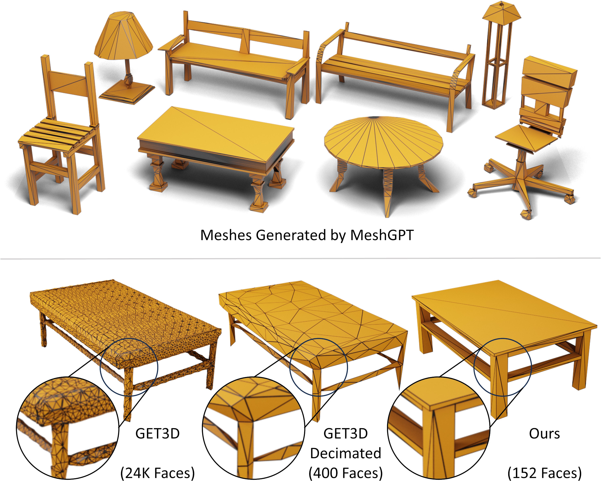
Recently, 3D vision research has seen great interest in generative 3D models using representations such as voxels Wu et al. 2016; Brock et al. 2016, point clouds Luo and Hu 2021; Zeng et al. 2022; Zhou et al. 2021, and neural fields Müller et al. 2023; Li et al. 2023; Liu et al. 2023; Gupta et al. 2023; Gao et al. 2022. However, these representations must then be converted into meshes through a post-process for use in downstream applications, for instance by iso-surfacing with Marching Cubes Lorensen and Cline 1998. Unfortunately, this results in dense, over-tessellated meshes that often exhibit oversmoothing and bumpy artifacts from the iso-surfacing, as shown in Figure 2. In contrast, artist-modeled 3D meshes are compact in representation, while maintaining sharp details with much fewer triangles.

Thus, we propose MeshGPT to generate a mesh representation directly, as a set of triangles. Inspired by powerful recent advances in generative models for language, we adopt a direct sequence generation approach to synthesize triangle meshes as sequences of triangles. Following text generation paradigms, we first learn a vocabulary of triangles. Triangles are encoded into latent quantized embeddings through an encoder. To encourage learned triangle embeddings to maintain local geometric and topological features, we employ a graph convolutional encoder. These triangle embeddings are then decoded by a ResNet He et al. 2016 decoder that processes the sequence of tokens representing a triangle to produce its vertex coordinates. We can then train a GPT-based architecture on this learned vocabulary to autoregressively produce sequences of triangles representing a mesh. Experiments across multiple categories of the ShapeNet dataset demonstrate that our method significantly improves 3D mesh generation quality in comparison with state of the art, with an average 9% increase in shape coverage and a 30-point improvement in FID scores.

Figure 2: Meshes generated by our method (top) for chairs, tables, benches, and lamps when trained on ShapeNet Chang et al. 2015. MeshGPT meshes tend to be compact, with the ability to represent both sharp details and curved boundaries. This contrasts with neural field-based approaches that yield dense triangulations not easily simplified through decimation (bottom).

In summary, our contributions are:

• A new generative formulation for meshes as a sequence of triangles, tailoring a GPT-inspired decoder-only transformer, to produce compact meshes with sharp edges.

• Triangles are represented as a vocabulary of latent geometric tokens to enable coherent mesh generation in an autoregressive fashion.

2 Related Work

Voxel-based 3D Shape Generation. Early shape generation approaches generated shapes as a grid of low-resolution voxels Wu et al. 2016; Choy et al. 2016; Jimenez Rezende et al. 2016; Brock et al. 2016 or, more recently, as high-resolution grids using efficient representations such as Octrees Tatarchenko et al. 2017 and sparse voxels Schwarz et al. 2022, with generative models such as GANs Goodfellow et al. 2020. These methods pioneered the extension of 2D generative techniques into the 3D domain. However, the voxel representation inherently constrains them with grid-like artifacts and high memory requirements, limiting their practical utility in capturing fine details and complex geometries.

Point Cloud Generation. Methods in this category represent 3D shapes by point samples on their surfaces, aiming to learn point distributions across shape datasets. Early works involved GANs for synthesizing point locations Li et al. 2018; Valsesia et al. 2018; Shu et al. 2019 and latent shape codes Achlioptas et al. 2018. Flow-based Yang et al. 2019 and gradient field-based models Cai et al. 2020 also yield impressive results. Recently, diffusion-based techniques have been adapted for point cloud generation Zhou et al. 2021; Zeng et al. 2022; Nichol et al. 2022, showing competitive performance in shape generation. However, point clouds, while useful, are not the ideal format for downstream applications requiring 3D content, as converting them to meshes, which apart from being non-trivial Peng et al. 2021; Sharp and Ovsjanikov 2020; Nan and Wonka 2017; Yang et al. 2018, can often fail to accurately reflect the characteristics of the underlying mesh datasets.

Neural Implicit Fields. Implicit representation of shapes as volumetric functions (e.g., signed distance functions) has become popular for encoding arbitrary topologies at any resolution Park et al. 2019; Mescheder et al. 2019. Various implicit generative methods have shown impressive performance using adversarial Chen and Zhang 2019; Shen et al. 2021 and diffusion-based Cheng et al. 2023; Gao et al. 2022; Müller et al. 2023 models. Diffusion-based neural field synthesis in MLP weight spaces Erkoç et al. 2023 and triplanes Shue et al. 2023 have also been explored, alongside leveraging image-based models for optimizing NeRFs Poole et al. 2022; Lin et al. 2023; Jain et al. 2022; Xu et al. 2023. However, like point clouds, these methods require mesh conversion Doi and Koide 1991; Lorensen and Cline 1998; Liao et al. 2018; Remelli et al. 2020; Shen et al. 2021 for downstream applications, often leading to dense meshes that don’t capture the properties of the underlying datasets (e.g., edge lengths, dihedral angles). In contrast, we directly fit a generative model to triangulated meshes, explicitly modeling the training data, resulting in clean, compact and coherent meshes as outputs.

3D Mesh Generation. While several discriminative approaches capable of learning signals directly on mesh structure were proposed over the recent years Gong et al. 2019; Sharp et al. 2022; Milano et al. 2020; Hu et al. 2022; Lim et al. 2018; Hanocka et al. 2019; Smirnov and Solomon 2021, direct mesh generation remains underexplored. Mesh generation has been approached with various learning-based methods Groueix et al. 2018; Dai and Nießner 2019; Chen et al. 2020; Nash et al. 2020. AtlasNet Groueix et al. 2018 and BSPNet Chen et al. 2020, for example, produce mesh patches and compact meshes through binary space partitioning, respectively. However, as we demonstrate in Sec. 4, these struggle with accurately capturing shape detail.

Closely related to our work, PolyGen Nash et al. 2020 employs two autoregressively trained networks to create explicit mesh structures. In contrast, our method utilizes a single decoder-only network, representing triangles through learned tokens for a more streamlined generation process compared to PolyGen’s separate vertex-and-face sequence approach. Additionally, we observe that PolyGen’s vertex generator, oblivious to face generation, and the face generator, not exposed to the generated vertex distribution during training, exhibit limited robustness during inference.

3 Method

Inspired by advancements in large language models, we develop a sequence-based approach to autoregressively generate triangle meshes as sequences of triangles. We first learn a vocabulary of geometric embeddings from a large collection of 3D object meshes, enabling triangles to be encoded to and decoded from this embedding. We then train a transformer for mesh generation as autoregressive next-index prediction over the learned vocabulary embeddings.

To learn the triangle vocabulary, we employ a graph convolution encoder operating on triangles of a mesh and their neighborhood to extract geometrically rich features that capture the intricate details of 3D shapes. These features are quantized as embeddings of a codebook using residual quantization Martinez et al. 2014; Juang and Gray 1982, effectively reducing sequence lengths of the mesh representation. These embeddings are sequenced and then decoded by a 1D ResNet He et al. 2016 guided by a reconstruction loss. This phase lays the groundwork for the subsequent training of the transformer.

We then train a GPT-style decoder-only transformer, which leverages these quantized geometric embeddings. Given a sequence of geometric embeddings extracted from the triangles of a mesh, the transformer is trained to predict the codebook index of the next embedding in the sequence. Once trained, the transformer can be auto-regressively sampled to predict sequences of embeddings. These embeddings can then be decoded to generate novel and diverse mesh structures that display efficient, irregular triangulations similar to human-crafted meshes.

3.1 Learning Quantized Triangle Embeddings

Figure 3: We employ a graph convolutional encoder to process mesh faces, leveraging geometric neighborhood information to capture strong features representing intricate details of 3D shapes. These features are then quantized into codebook embeddings using residual quantization Juang and Gray 1982; Martinez et al. 2014. In contrast to naive vector quantization, this ensures better reconstruction quality. The quantized embeddings are subsequently sequenced and decoded through a 1D ResNet He et al. 2016, guided by a reconstruction loss.

Autoregressive generative models, such as transformers, synthesize sequences of tokens where each new token is conditioned on previously generated tokens. For generating meshes using transformers, we must then define the ordering convention of generation, along with the tokens.

For sequence ordering, Polygen Nash et al. 2020 suggests a convention where faces are ordered based on their lowest vertex index, followed by the next lowest, and so forth. Vertices are sorted in $z$-$y$-$x$ order ($z$ representing the vertical axis), progressing from lowest to highest. Within each face, indices are cyclically permuted to place the lowest index first. In our method, we also adopt this sequencing approach.

To define the tokens to generate, we consider a practical approach to represent a mesh $\mathcal{M}$ for autoregressive generation: a sequence of triangles,

$$\mathcal{M}:=(f_{1},f_{2},f_{3},\ldots,f_{N}),$$ (1)

with $N$ faces (triangles), $f_{i}\in\mathbb{R}^{n_{\text{in}}}$ having $n_{\text{in}}$ features. A simple approach to describe each triangle is as its three vertices, comprising nine total coordinates. Upon discretization, these coordinates can be treated as tokens. The sequence length in this case would be $9N$.

However, we observe two major challenges when using coordinates directly as tokens. First, the sequence lengths become excessively long, as each face is represented by nine values. This length does not scale well with transformer architectures, which often have limited context windows. Second, representing discrete positions of a triangle as tokens fails to capture geometric patterns effectively. This is because such a representation lacks information about neighboring triangles and does not incorporate any priors from mesh distributions.

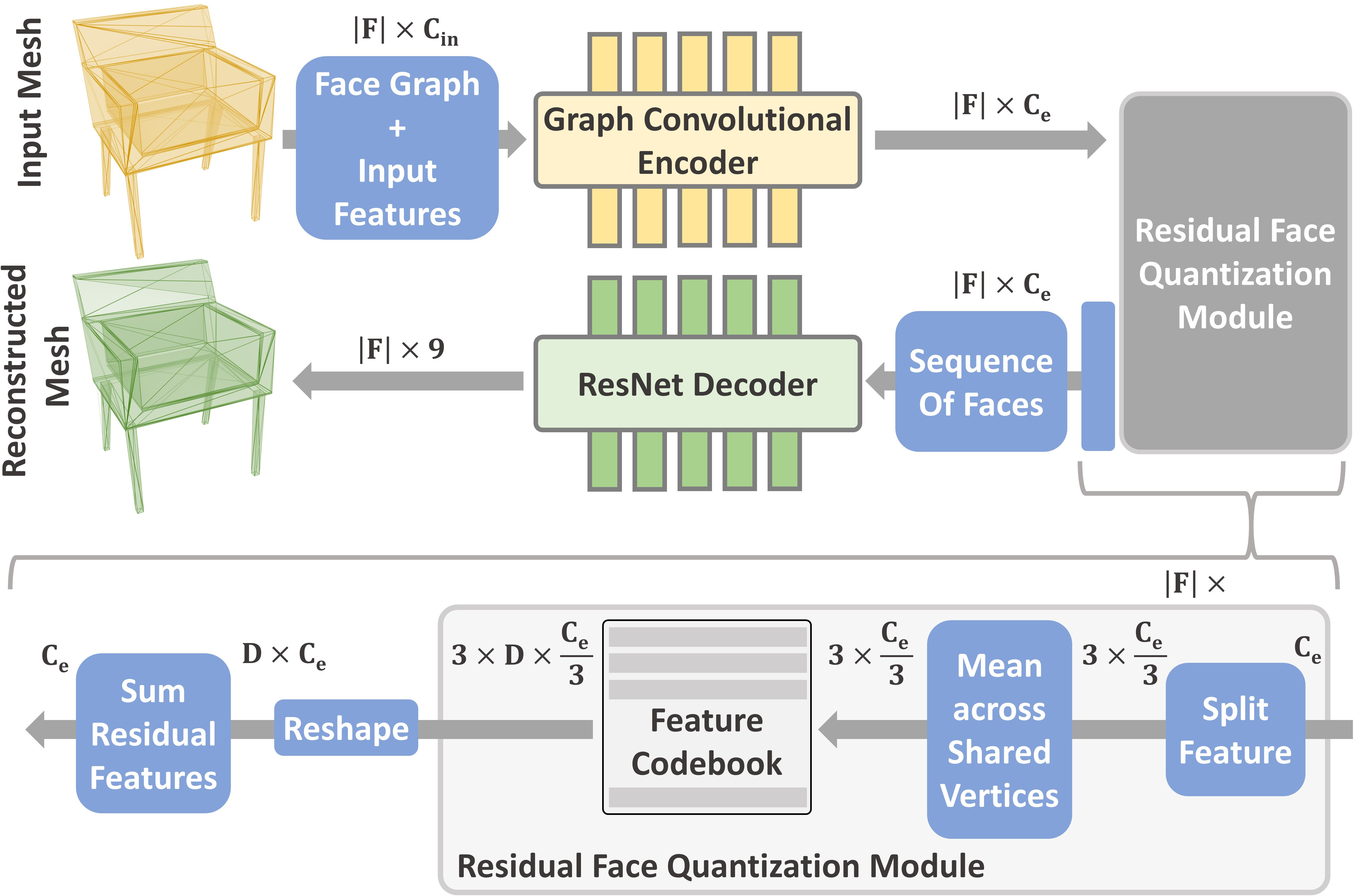
To address the aforementioned challenges, we propose to learn geometric embeddings from a collection of triangular meshes, utilizing an encoder-decoder architecture with residual vector quantization at its bottleneck (Fig. 3).

The network’s encoder $E$ employs graph convolutions on mesh faces, where each face forms a node and neighboring faces are connected by undirected edges. The input face node features are comprised of the nine positionally encoded coordinates of its vertices, face normal, angles between its edges, and area. These features undergo processing through a stack of SAGEConv Hamilton et al. 2017 layers, extracting a feature vector for each face. This graph convolutional approach enables the extraction of geometrically enriched features $z_{i}\in\mathbb{R}^{n_{\text{z}}}$ for each face,

$$\mathbf{Z}=(z_{1},z_{2},\ldots,z_{N})=E(\mathcal{M}),$$ (2)

fusing neighborhood information into the learned embeddings.

For quantization, we employ residual vector quantization (RQ) Martinez et al. 2014. We found that using a single code per face is insufficient for accurate reconstruction. Instead, we use a stack of D codes per face. Further, we find that instead of directly using D codes per face, it is more effective to first divide the feature channels among the vertices, aggregate the features by shared vertex indices, and then quantize these vertex-based features, giving $\frac{\text{D}}{3}$ codes per vertex, and therefore effectively D codes per face. This leads to sequences that are easier to learn for the transformer trained subsequently (see Tab. 3 and Fig. 10 for comparison). Formally, given a codebook $\mathcal{C}$, RQ with depth D represents features $\mathbf{Z}$ as

$$\mathbf{T}=(t_{1},t_{2},\ldots,t_{N})=\text{RQ}\,(\mathbf{Z};\mathcal{C},D),$$ (3)

$$t_{i}=(t_{i}^{1},t_{i}^{2},\ldots,t_{i}^{D}),$$ (4)

where $t_{i}$ is a stack of tokens, each token $t_{i}^{d}$ being an index to an embedding $\mathbf{e}(t_{i}^{d})$ in the codebook $\mathcal{C}$.

The decoder then decodes the quantized face embeddings to triangles. First, the stack of D features is reduced to a single feature per face through summation across embeddings and concatenation across vertices,

$$\mathbf{\hat{Z}}=(\hat{z}_{1},\ldots,\hat{z}_{N}),\;\text{with}\;\hat{z}_{i}=\oplus_{v=0}^{2}\sum_{d=1}^{\frac{D}{3}}{\,\mathbf{e}(t_{i}^{3.v+d})}.$$ (5)

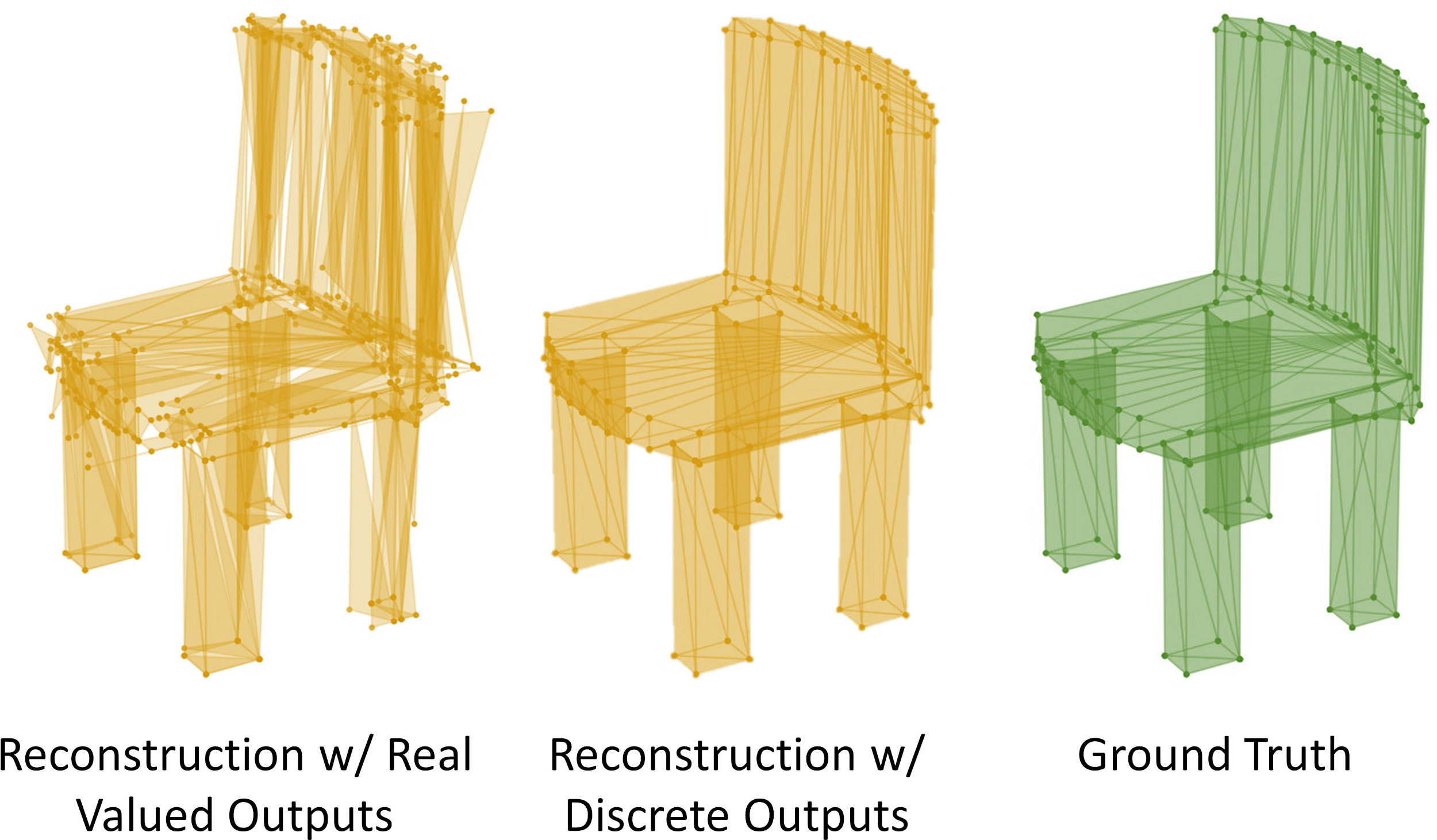
The face embeddings are arranged in the previously described order, and a 1D ResNet34 decoding head $G$ processes the resulting sequence to output the reconstructed mesh $\hat{\mathcal{M}}=G(\mathbf{\hat{Z}})$ with $9$ coordinates representing each face. We observe that predicting these coordinates as discrete variables, i.e. as a probability distribution over a set of discrete values, leads to a more accurate reconstruction compared to regressing them as real values (Fig. 4). A cross-entropy loss on the discrete mesh coordinates and a commitment loss for the embeddings guides the reconstruction process. More details can be found in supplementary.

Figure 4: Our method utilizes a ResNet He et al. 2016 decoder that outputs mesh faces as a distribution over discretized coordinate values (center), as opposed to regression of continuous values (left). This significantly reduces floating face artifacts, leading to reconstructions that more closely resemble the ground truth (right).

After training, the graph encoder $E$ and codebook $\mathcal{C}$ are incorporated into the transformer training, using $\mathbf{T}$ from Eq. 3 as the token sequence. With $|\mathbf{T}|=DN$, this sequence is more concise than the naive $9N$-length tokenization when $D<9$. Thus, we obtain geometrically rich embeddings with shorter sequence lengths, overcoming our initial challenges and paving the way for efficient mesh generation.

3.2 Mesh Generation with Transformers

Figure 5: We employ a transformer to generate mesh sequences as token indices from a pre-learned codebook vocabulary. During training, a graph encoder extracts features from mesh faces, which are quantized into a set of face embeddings. These embeddings are flattened, bookended with start and end tokens, and fed into a GPT-style transformer. This decoder predicts the subsequent codebook index for each embedding, optimized via cross-entropy loss.

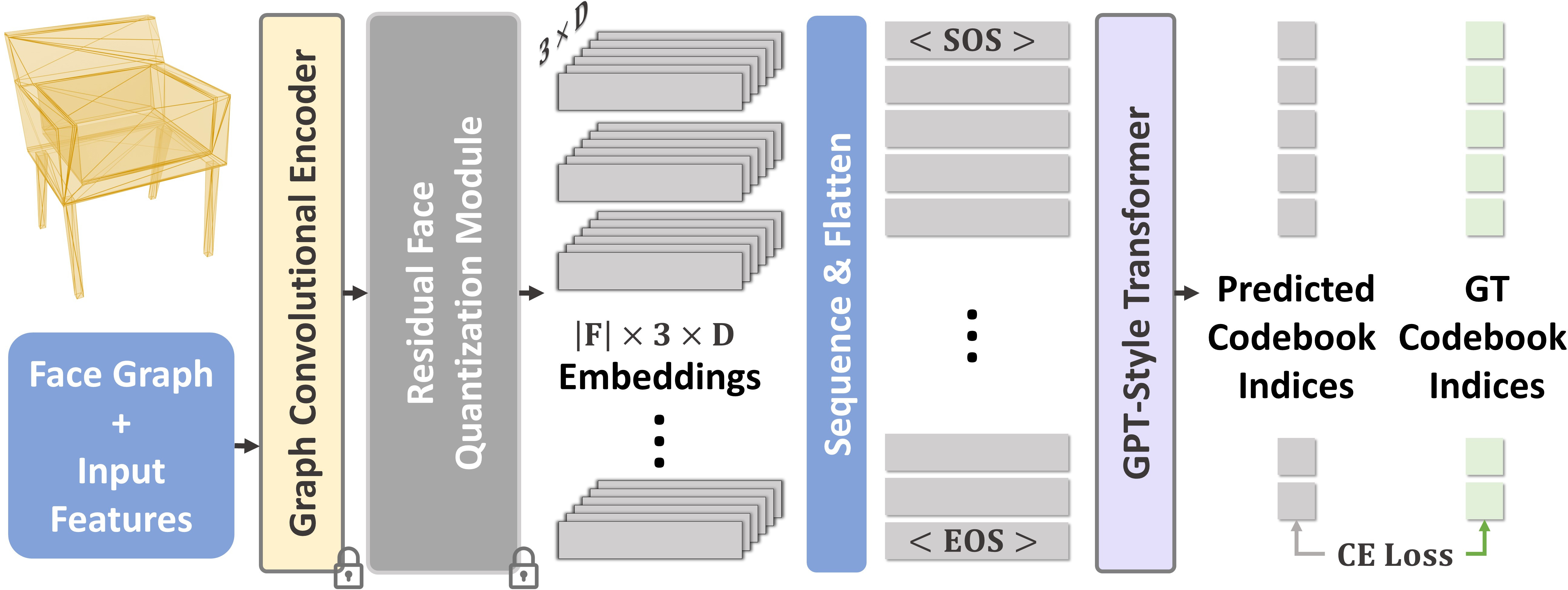
We employ a decoder-only transformer architecture from the GPT family of models to predict meshes as sequences of indices from the learned codebook in Sec. 3.1. The input to this transformer consists of embeddings $\mathbf{e}(t_{i}^{d})$ extracted from the mesh $\mathcal{M}$ using the GraphConv encoder $E$ and quantized using RQ (Eq. 3). The embeddings are prefixed and suffixed with a learned start and end embedding. Additionally, learned discrete positional encodings are added, indicating the position of each face in the sequence and the index of each embedding within the face. The features then pass through a stack of multiheaded self-attention layers, where the transformer is trained to predict the codebook index of the next embedding in the sequence (Fig. 5). Essentially, we maximize the log probability of the training sequences with respect to the transformer parameters $\theta$,

$$\prod_{i=1}^{N}\prod_{d=1}^{D}p\,(t_{i}^{d}\,|\,\mathbf{e}(t_{<i}^{d}),\,\mathbf{e}(t_{i}^{<d});\,\theta).$$ (6)

Once the transformer is trained, it can autoregressively generate a sequence of tokens, starting with a start token and continuing until a stop token is encountered using beam sampling. The codebook embeddings indexed by this sequence of tokens is then decoded by decoder $G$ to produce the generated mesh. As this output initially forms a ‘triangle soup’ with duplicate vertices for neighboring faces, we apply a simple post-processing operation to merge close vertices (e.g., with MeshLab), to yield the final mesh.

3.3 Implementation Details

In learning the triangle vocabulary, our residual quantization layer features a depth of 2, yielding $D=6$ embeddings per face, each with dimension 192. The codebook is dynamically updated using an exponential moving average of the clustered features. Following Lee et al. 2022, we incorporate stochastic sampling of codes and employ a shared codebook across all levels. The decoder predicts the coordinates of the faces across 128 classes, resulting in a discretization of space to $128^{3}$ possible values. This encoder-decoder network is trained using 2 A100 GPUs for $\approx$ 2 days.

For our transformer, we use a GPT2-medium model, equipped with a context window of up to 4608 embeddings. The model is trained on 4 A100 GPUs, for $\approx$ 5 days.

Both the encoder-decoder network and the transformer are written using the Pytorch  Paszke et al. 2019 and are trained utilizing the ADAM optimizer Kingma and Ba 2014. We set the learning rate at $1\times 10^{-4}$ and use an effective batch size of 64.

4 Experiments

4.1 Dataset and Metrics

Data. We present our results on the ShapeNetV2 dataset. Both the encoder-decoder network and the GPT model are trained across all 55 categories of this dataset. Additionally, we fine-tune the GPT model specifically on four categories: Chair, Table, Bench, and Lamp. The results are reported on these categories. During training, we employ augmentation techniques including random shifts and random scaling to enhance the diversity of the training meshes. Similar to Polygen Nash et al. 2020, we also apply planar decimation to further augment the shapes. To ensure that the entire mesh fits into the transformer’s context window, we select only those meshes for training that have fewer than 800 faces post-decimation. Detailed information regarding the augmentation processes, decimation techniques, and data splits are provided in the supplementary material.

Metrics. Evaluating the unconditional synthesis of 3D shapes presents challenges due to the absence of direct ground truth correspondence. Hence, we utilize established metrics for assessment, consistent with previous works Zeng et al. 2022; Luo and Hu 2021; Zhou et al. 2021. These include Minimum Matching Distance (MMD), Coverage (COV), and 1-Nearest-Neighbor Accuracy (1-NNA). For MMD, lower is better; for COV, higher is better; for 1-NNA, 50% is the optimal. We use a Chamfer Distance (CD) distance measure for computing these metrics in 3D. More details about these metrics can be found in the supplementary.

The aforementioned metrics effectively measure the quality of shapes but do not address the visual similarity of the generated meshes to the real distribution. To assess this aspect, we render both the generated meshes and the ShapeNet meshes as images from eight different viewpoints using Blender, applying a metallic material to emphasize the geometric structures. Subsequently, we calculate the FID (Fréchet Inception Distance) and KID (Kernel Inception Distance) scores for these image sets. For both FID and KID, lower scores indicate better performance. We further report compactness as the average number of vertices and faces in the generated meshes.

4.2 Results

Class	Method	COV$\uparrow$	MMD$\downarrow$	1-NNA	FID$\downarrow$	KID$\downarrow$	$\mid$V$\mid$	$\mid$F$\mid$
Chair	AtlasNet Groueix et al. 2018	9.03	4.05	95.13	170.71	0.169	2500	4050
	BSPNet Chen et al. 2020	16.48	3.62	91.75	46.73	0.030	673	1165
	Polygen Nash et al. 2020	31.22	4.41	93.56	61.10	0.043	248	603
	GET3D Gao et al. 2022	40.85	3.56	83.04	81.45	0.054	13725	27457
	GET3D*	38.75	3.57	84.07	78.29	0.065	199	399
	MeshGPT	43.28	3.29	75.51	18.46	0.010	125	228
Table	AtlasNet Groueix et al. 2018	7.16	3.85	96.30	161.38	0.150	2500	4050
	BSPNet Chen et al. 2020	16.83	3.14	93.58	30.78	0.017	420	699
	Polygen Nash et al. 2020	32.99	3.00	88.65	38.53	0.029	147	454
	GET3D Gao et al. 2022	41.70	2.78	85.54	93.93	0.076	13767	27537
	GET3D*	37.95	2.85	81.93	50.46	0.037	199	399
	MeshGPT	45.68	2.36	72.88	6.24	0.002	99	187
Bench	AtlasNet Groueix et al. 2018	20.53	2.47	90.58	189.39	0.163	2500	4050
	BSPNet Chen et al. 2020	28.74	2.05	88.44	59.11	0.030	457	756
	Polygen Nash et al. 2020	51.92	1.97	76.98	49.34	0.031	172	430
	MeshGPT	55.23	1.44	68.24	8.72	0.001	159	291
Lamp	AtlasNet Groueix et al. 2018	19.97	4.68	91.85	177.91	0.139	2500	4050
	BSPNet Chen et al. 2020	18.38	5.32	93.13	112.65	0.077	587	1011
	Polygen Nash et al. 2020	47.86	4.18	81.42	52.48	0.025	185	558
	MeshGPT	53.88	3.94	65.73	19.91	0.004	150	288

Table 1: Quantitative comparison on the task of unconditional mesh generation on a subset of categories from the ShapeNet Chang et al. 2015 dataset. GET3D* refers to meshes simplified to 400 faces using QEM Garland and Heckbert 1997. MMD values are multiplied by $10^{3}$. We outperform the baselines on shape quality, visual and compactness metrics.

Figure 6: Qualitative comparison of Chair and Table meshes from ShapeNet Chang et al. 2015. Our approach produces compact meshes with sharp geometric details. In contrast, baselines often either miss these details, produce over-triangulated meshes, or output too simplistic shapes.

Figure 7: Qualitative comparison of Bench and Lamp meshes from the ShapeNet Chang et al. 2015 dataset. Compared to baselines, our method produces valid meshes with high geometric fidelity.

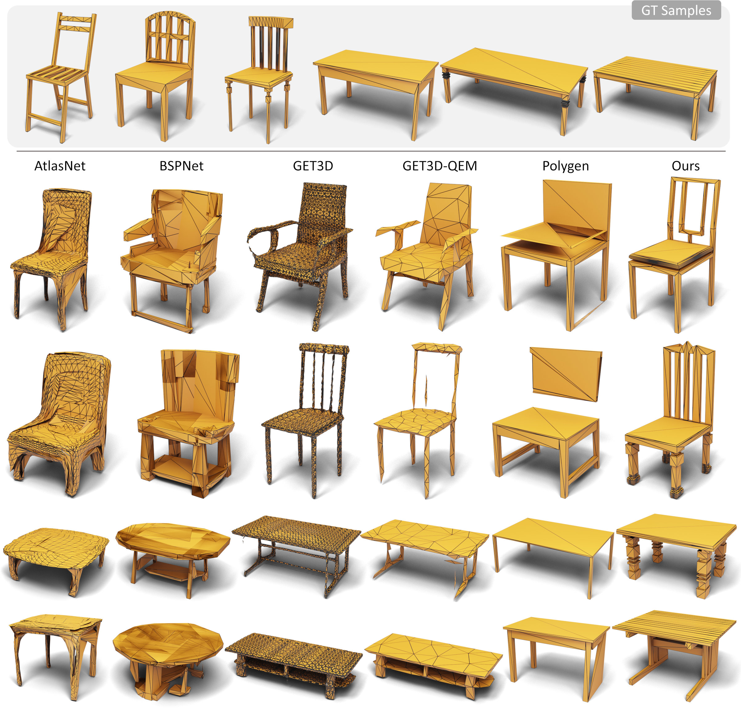
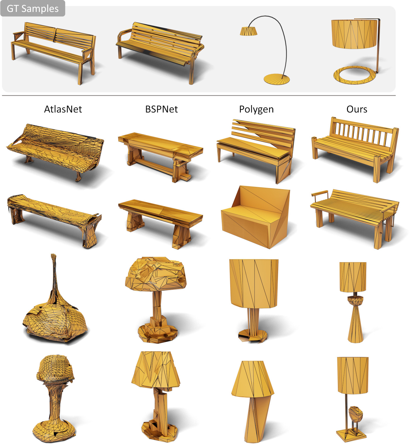
We benchmark our approach against leading mesh generation methods: Polygen Nash et al. 2020, which generates polygonal meshes by first generating vertices followed by faces conditioned on the vertices; BSPNet Chen et al. 2020, which represents a mesh through convex decompositions; and AtlasNet Groueix et al. 2018, which represents a 3D mesh as a deformation of multiple 2D planes. We additionally compare with a state-of-the-art neural field-based method, GET3D Gao et al. 2022, that creates shapes as 3D signed distance fields (SDFs) from which a mesh is extracted by differentiable marching tetrahedra. For BSPNet and AtlasNet, which are built on autoencoder backbones, we follow Achlioptas et al. 2018 to fit a Gaussian mixture model with 32 components to enable unconditional sampling of shapes.

As shown in Fig. 6, Fig. 7 and Tab. 1, our method outperforms all baselines in all four categories. Our method can generate sharp and compact meshes with high geometric details. Compared to Polygen, our approach creates shapes with more intricate details. Additionally, Polygen’s separate training for vertex and face models, with the latter only exposed to ground truth vertex distributions, makes it more susceptible to error accumulation during inference. AtlasNet often suffers from folding artifacts, resulting in lower diversity and shape quality. BSPNet’s use of BSP tree of planes tends to produce blocky shapes with unusual triangulation patterns. GET3D generates good high-level shape structures, but over-triangulated and with imperfect flat surfaces. Simplifying GET3D-generated meshes with algorithms such as QEM Garland and Heckbert 1997 results in a loss of fine structures.

User Study. We further conducted a user study, in Tab. 2, to assess generated mesh quality. 49 participants were shown pairs of four meshes, randomly selected from our method and each baseline method. Additionally, users were presented with ground truth ShapeNet meshes for comparison. Participants were asked their preference between our method and the baseline in terms of both overall shape quality and similarity of triangulation patterns to the ground truth meshes. This resulted in 784 total question responses. Our method was significantly preferred over AtlasNet, Polygen, and BSPNet in both shape and triangulation quality. Moreover, a majority of users (68%) favored our method over neural field-based GET3D in shape quality, with even higher preference (73%) for triangulation quality. This underscores our ability to generate high-quality meshes that align with human users’ preferences. Further user study details are provided in the supplemental.

Figure 8: Shape novelty analysis on ShapeNet Chang et al. 2015 chair category. We show the 3 nearest neighbors in terms of Chamfer Distance (CD) for a generated shape (top). We also plot the distribution of 500 generated chair samples from our method and their closeness to training distribution. Our method can generate shapes that are similar (low CD) as well as different (high CD) from the training distribution, with shapes at the $50^{\text{th}}$ percentile looking different from closest train shape.

Figure 9: Given a partial mesh, our method can infer multiple possible shape completions.

Preference	AtlasNet Groueix et al. 2018	BSPNet Chen et al. 2020	Polygen Nash et al. 2020	GET3D Gao et al. 2022
Our Shape	82.65%	78.57%	85.71%	68.37%
Our Triangulation	84.69%	71.43%	84.69%	73.47%

Table 2: Percentage of users who prefer our method over the baselines in terms of shape quality and the triangulation quality. Our generated meshes are preferred significantly more often.

Method	COV$\uparrow$	MMD$\downarrow$	1-NNA	FID$\downarrow$	KID$\downarrow$
w/o Learned Tokens	27.50	4.51	93.15	40.20	0.024
w/o Encoder Features	39.24	3.43	84.48	30.35	0.017
w/o Pretraining	36.97	3.73	84.69	27.54	0.014
w/o Sequence Compression	30.98	4.15	88.98	38.76	0.023
w/o per Vertex Quantization	23.57	5.49	98.35	74.94	0.050
MeshGPT	43.28	3.29	75.51	18.46	0.010

Table 3: Ablations of our design choices on the Chair category of the ShapeNet Chang et al. 2015 dataset. As highlighted by the drop in performance by removing any of them, each of these contribute to the final method.

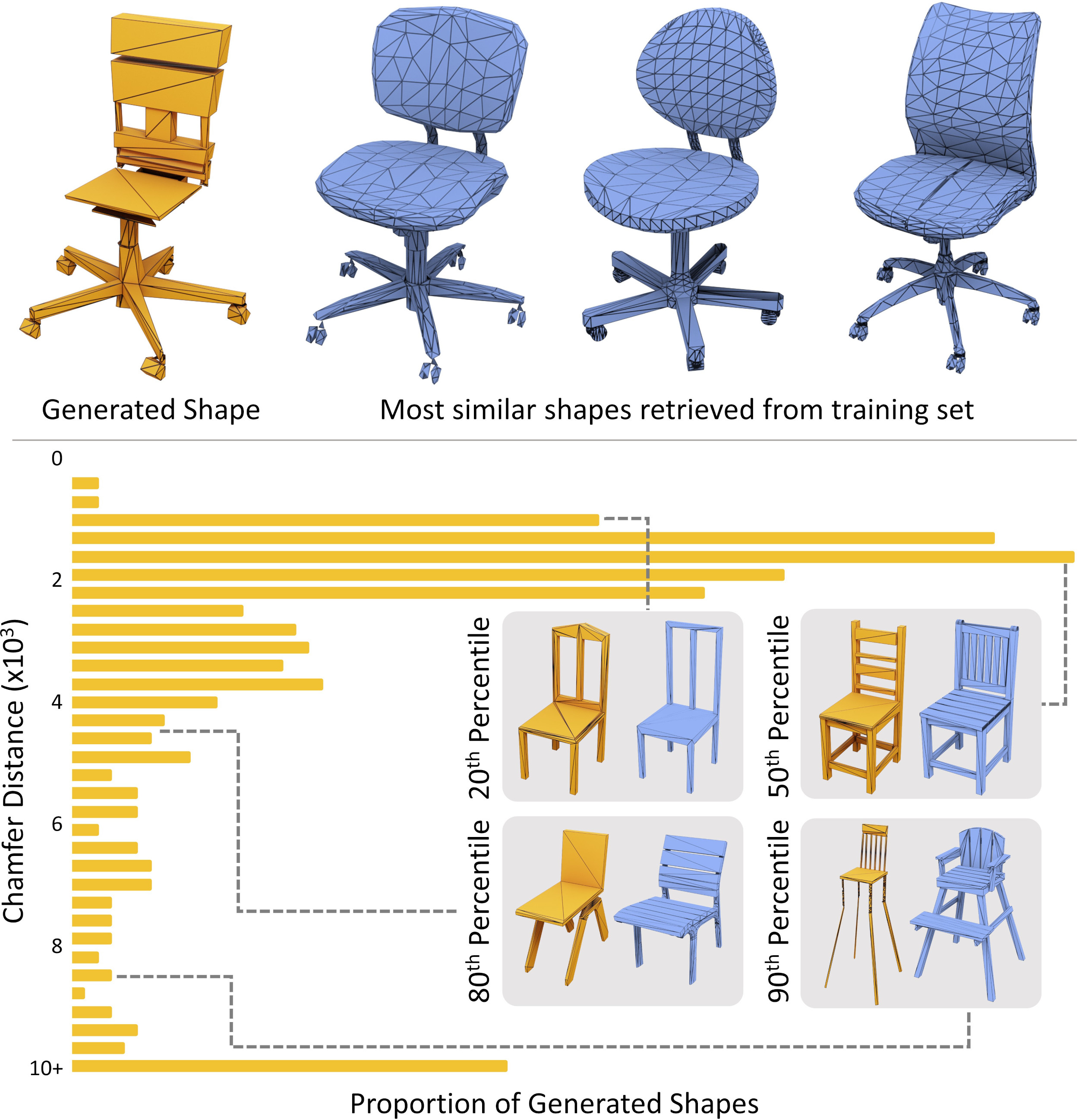
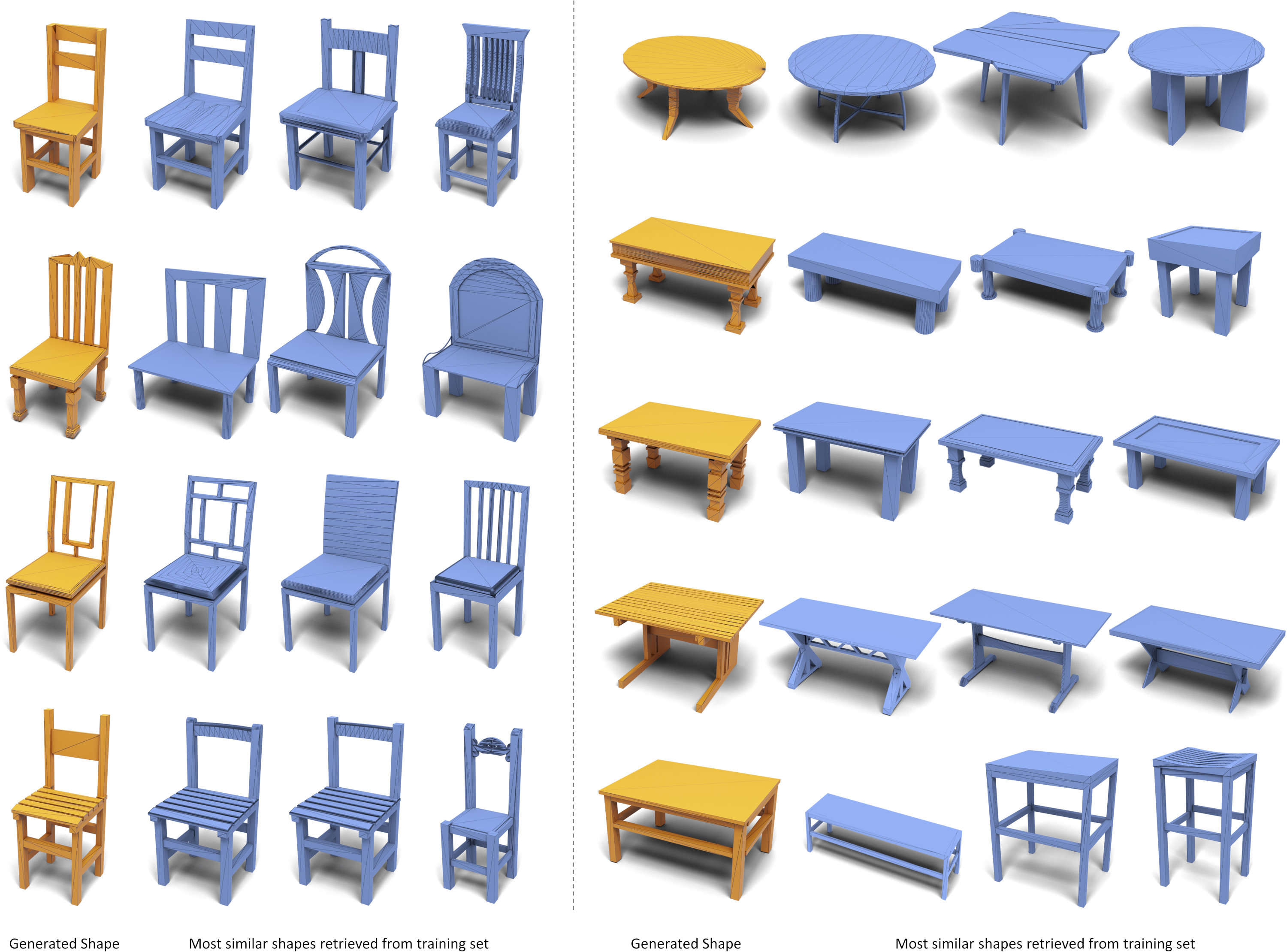
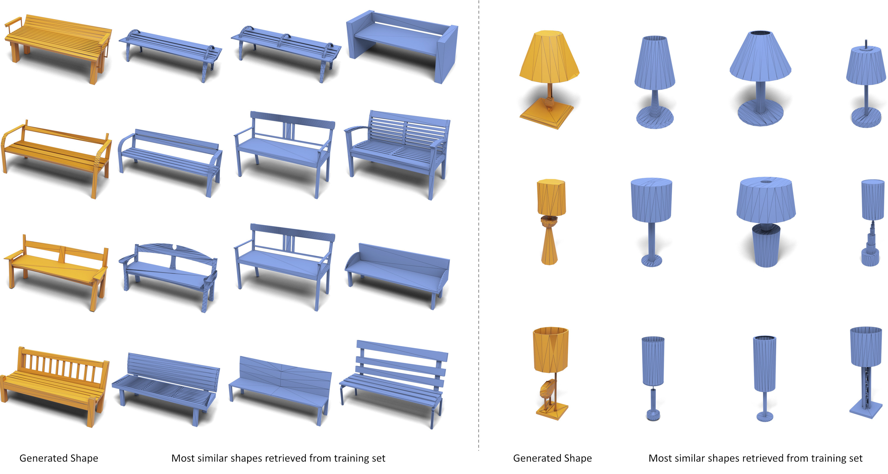
Shape Novelty Analysis. We investigate whether our method can generate novel shapes that extend beyond the training dataset, ensuring the model is not merely retrieving existing shapes. Following the methodology in previous studies Erkoç et al. 2023; Hui et al. 2022, we generate 500 shapes using our model. For each generated shape, we identify the top three nearest neighbors from the training set based on Chamfer Distance (CD). To ensure a fair distance computation, accounting for potential discrepancies due to scale or shift in the augmented generations, we normalize all generated and train shapes to be centered within $[0,1]^{3}$.

Fig. 8 displays the most similar shapes from the train set corresponding to a sample generated by our model. We conduct a detailed analysis of the shape similarity distribution between the retrieved and generated shapes on the Chair category in Fig. 8. The CD distribution reveals that our method not only covers shapes in the training set, indicated by low CD values, but also successfully generates novel and realistic-looking shapes, indicated by high CD values. In the supplemental, we present further analysis of the novelty of all meshes generated by our method, which are featured in the figures of this paper.

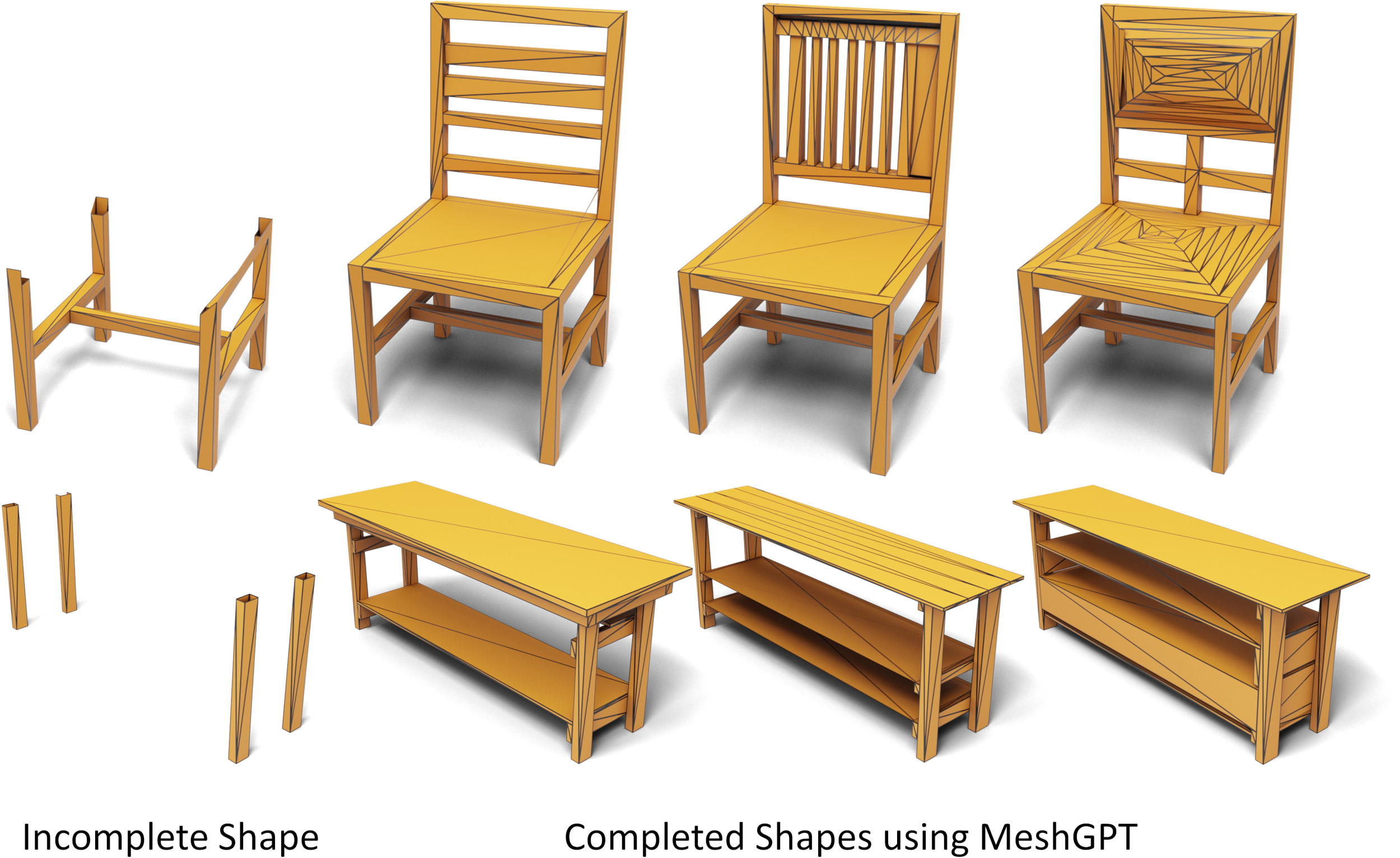
Shape Completion. Our model can infer multiple possible completions for a given partial shape, leveraging its probabilistic nature to generate diverse shape hypotheses. Fig. 9 illustrates examples of chair and table completions.

4.2.1 Ablations

In Tab. 3, we show a set of ablations on the task of unconditional mesh generation on ShapeNet Chair category. Further ablations are detailed in the supplementary.

Figure 10: Ablation over our method’s components. Naive tokenization (w/o Learned Tokens) and naive per face quantization (w/o per-vertex quantization) markedly diminishes shape quality. Longer sequences without sequence compression (w/o Sequence Compression) lead to the model forgetting the context and repeating shape elements in the output.

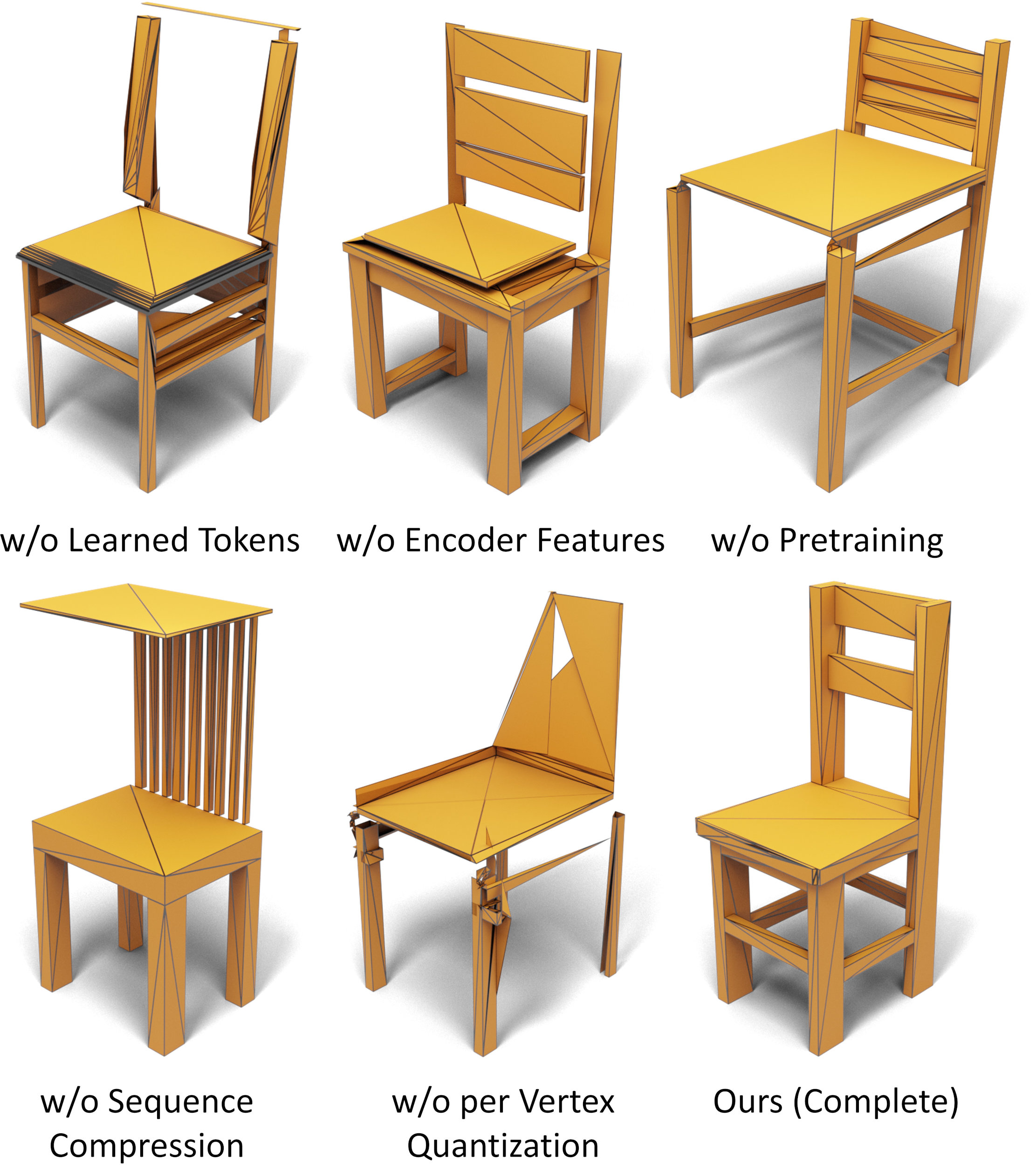
Do learned geometric embeddings help? Using our geometric embeddings in vocabulary learning significantly improves over naive coordinate tokenization (w/o Learned Tokens), as shown in Tab. 3 and Fig. 3.

Does sequence length compression help? As evidenced by Tab. 3 and Fig. 3, a model with a shorter sequence length performs better than without (w/o Sequence Compression), as shorter sequence lengths fit transformer context windows better. Visually, with longer sequences, shapes exhibit repeating structures due to limited context.

What is the effect of aggregation and quantization across vertex indices instead of faces? As discussed in Section 3, an alternative to having embeddings aggregated and quantized across vertex indices, is to simply have the same number of embeddings directly per face (w/o per Vertex Quantization). In Tab. 3, we observe that this makes sequences much harder to learn with the transformer.

Do features from graph convolutional encoder help in mesh generation? An alternative to using embeddings from the graph encoder and the codebook is to only use the codebook indices of these tokens as input to the transformer, and let the transformer learn the discrete token embeddings (w/o Encoder Features). While the transformer is able to still learn meaningful embeddings, these are still not as effective as using graph encoder features.

What is the effect of large-scale shape pretraining? Tab. 3 shows that training only on shapes from individual categories (w/o Pretraining) leads to overfitting and subobtimal performance, in contrast to pre-training our GPT transformer on all ShapeNet train shapes.

Limitations. MeshGPT significantly advances direct mesh generation but faces several limitations. Its autoregressive nature leads to slower sampling performance, with mesh generation times taking 30 to 90 seconds. Despite our learned tokenization approach reducing sequence lengths, which suffices for single object generation, it may not be as effective for scene-scale generation, suggesting an area for future enhancement. Moreover, our current computational resources limit us to using a GPT2-medium transformer, which is smaller than more sophisticated models like Llama2 Touvron et al. 2023. Given that larger language models benefit from increased data and computational power, expanding these resources could significantly boost MeshGPT’s performance and capabilities.

5 Conclusion

We have introduced MeshGPT, a novel shape generation approach that outputs meshes directly as triangles. We learn a vocabulary of geometric embeddings over a distribution of meshes, over which a transformer is trained to predict meshes autoregressively as a sequence of triangles. In contrast to existing mesh generation approaches, our method generates clean, coherent meshes which are compact and follow the triangulation patterns in real data more closely. We believe that MeshGPT will not only elevate the current landscape of mesh generation but also inspire new research in the area, offering a unique alternative to the more commonly explored representations for 3D content creation.

Appendix

In this supplementary document, we discuss additional details about our method MeshGPT. We provide implementation details of our method, loss functions, and the baselines in Section B. Additional details about the user study are provided in Section C. We also provide further qualitative and quantitative results (Section E), including a shape novelty analysis (Section D) for shapes from the main paper. We further encourage the readers to check out the supplemental video for a summary of the method and an overview of results.

Appendix A Data

Selection. We use the ShapeNetV2 Chang et al. 2015 dataset for all our experiments. We first apply planar decimation to each shape using Blender Community 2018, with the angle tolerance parameter $\alpha$ set within $[1,60]$. The impact of this decimation is assessed by calculating the Hausdorff distance Blumberg 1920 between the decimated and original shapes. We then choose, for each original shape, the decimated version with the Hausdorff distance closest to, but below, a pre-set threshold $\delta_{\text{hausdorff}}$. Shapes with more than 800 faces are excluded, resulting in a final count of 28980 shapes across all categories. The Chair, Table, Bench, and Lamp categories are further divided into a 9:1 train-test split. All shapes from rest of the categories are used for pretraining phase, while only the training subset from specific categories is used for pretraining and finetuning. All shapes are normalized to be centered at the origin and scaled to ensure the longest side is of unit length.

Figure 11: Additional novel shapes on Chairs, Tables, Benches and Lamps generated by our method.

Figure 12: Shape novelty analysis on ShapeNet Chang et al. 2015 chair and table category for shapes generated by our method shown in main paper. We show the 3 nearest neighbors in terms of Chamfer Distance (CD) for a generated shape. Shapes are scaled to a unit length along all axes to account for augmented generations before computing CD.

Figure 13: Shape novelty analysis on ShapeNet Chang et al. 2015 bench and lamp category for shapes generated by our method shown in main paper. We show the 3 nearest neighbors in terms of Chamfer Distance (CD) for a generated shape. Shapes are scaled to a unit length along all axes to account for augmented generations before computing CD.

Augmentation. During the training of both the encoder-decoder and the transformer, multiple augmentation techniques are applied to all train shapes. Scaling augmentation, ranging from $0.75$ to $1.25$, is independently applied across each axis. Post-scaling, meshes are resized to keep the longest side at unit length. Additionally, jitter-shift augmentation in the range of $[-0.1,0.1]$ is used, adjusted to maintain the mesh within the unit bounding box around the origin. We also implement varying levels of planar decimation for training shapes, provided the distortion remains below $\delta_{\text{hausdorff}}$.

Appendix B Method Details

B.1 Architecture

Figure 14: Our encoder-decoder network features an encoder with SAGEConv Hamilton et al. 2017 layers processing mesh faces as a graph. Each node inputs positionally encoded face triangle coordinates, area, edge angles, and normal. The decoder, a 1D ResNet-34 He et al. 2016, interprets face features as a sequence, outputting logits for the discretized face triangle coordinates in a $128^{3}$ space.

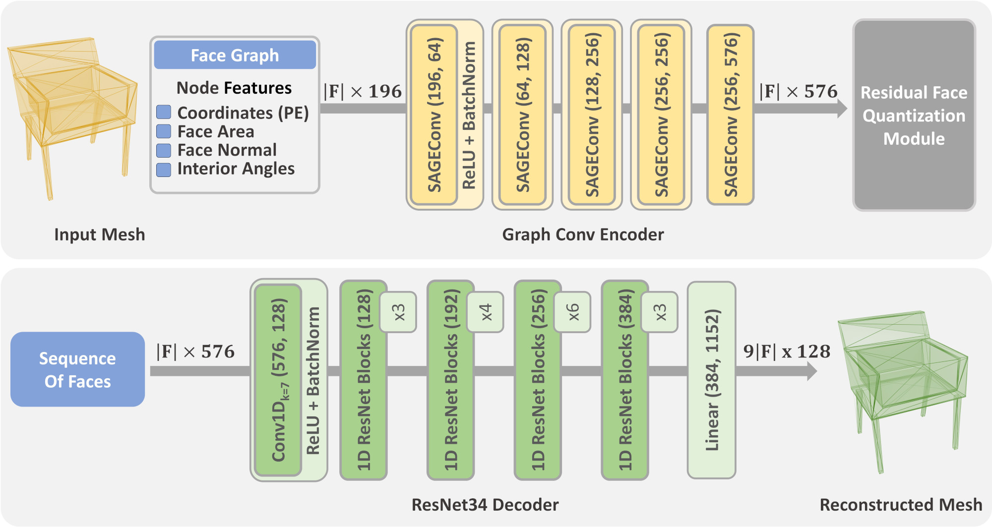
The architecture of our encoder-decoder network is elaborated in Fig. 14. The encoder comprises a series of SAGEConv Hamilton et al. 2017 graph convolution layers, processing the mesh in the form of a face graph. For each graph node, input features include the positionally encoded 9 coordinates of the face triangle, its area, the angles between its edges, and the normal of the face. The decoder is essentially a 1D ResNet-34 He et al. 2016 network, applied to the face features interpreted as a 1D sequence. It outputs logits corresponding to the 9 discrete coordinates of each face triangle, which are discretized within a $128^{3}$ space. The codebook $\mathcal{C}$ has a size of $16384$. The architecture of the transformer is simply a GPT-2 medium architecture, i.e. $24$ multi-headed self attention layers, $16$ heads, $768$ as feature width, with context length of $4608$.

B.2 Residual Vector Quantization

Fundamentals. For quantization, we employ residual vector quantization (RQ) Martinez et al. 2014; Lee et al. 2022. RQ discretizes a vector $\mathbf{z}$ with a stack of $D$ ordered codes. Starting with the $0^{\text{th}}$ residual $\mathbf{r}^{0}=\mathbf{z}$, RQ recursively computes $t^{d}$ as the code of the residual $\mathbf{r}^{d-1}$, and the next residual $\mathbf{r}^{d}$ as

$$t^{d} =\mathcal{Q}\,(\mathbf{r}^{d-1};\mathcal{C})$$ (7)

$$\mathbf{r}^{d} =\mathbf{r}^{d-1}-\mathbf{e}(t^{d})$$ (8)

where $\mathcal{Q}(\mathbf{z};\mathcal{C})$ denotes vector quantization of $\mathbf{z}$ with codebook $\mathcal{C}$, and $\mathbf{e}(t^{d})$ is the embedding in the codebook $\mathcal{C}$. Further, we define

$$\hat{\mathbf{z}}^{(d)}=\sum_{1}^{d}{\,\mathbf{e}(t^{d})}$$ (9)

as the partial sum of up to $d$ code embeddings, and $\hat{\mathbf{z}}=\hat{\mathbf{z}}^{D}$ is the quantized vector of $\mathbf{z}$. The recursive quantization of RQ thus approximates the vector $\mathbf{z}$ in a coarse-to-fine manner Lee et al. 2022. The commitment loss can now be defined between vector $\mathbf{z}$ and its quantization $\hat{\mathbf{z}}$ as

$$\mathcal{L}_{\text{commit}}(\mathbf{z},\hat{\mathbf{z}})=\sum_{d=1}^{D}\|\mathbf{z}-\text{sg}[\hat{\mathbf{z}}^{(d)}]\|_{2}^{2}$$ (10)

where sg denotes the stop gradient operation.

Per Vertex Residual Vector Quantization. Instead of directly applying RQ, for a face feature $\mathbf{z_{i}}$ extracted by the graph encoder, we first split this $576$ dimension face feature $\mathbf{z_{i}}$ into 3 features, $(\mathbf{z}_{i}^{1},\mathbf{z}_{i}^{2},\mathbf{z}_{i}^{3})$, each of $192$ dimensions representing the features of the face triangle’s 3 vertices. The features the fall on vertices that are shared across faces are averaged. On these per vertex index feature $\mathbf{z}_{i}^{j}$, RQ quantizes them into a stack of $\frac{D}{3}$ features,

$$\text{RQ}(\mathbf{z_{i}};\mathcal{C},D)=(\text{RQ}(\mathbf{z}^{1}_{i};\mathcal{C},\frac{D}{3}),\ldots,\text{RQ}(\mathbf{z}^{3}_{i};\mathcal{C},\frac{D}{3}))$$ (11)

for codebook $\mathcal{C}$, with

$$\text{RQ}(\mathbf{z^{j}_{i}};\mathcal{C},\frac{D}{3})=(t^{2j-\frac{D}{3}+1}_{i},t^{2j-\frac{D}{3}+2}_{i},\ldots,t^{2j}_{i}),$$ (12)

where $t^{d}_{i}$ is the index to the embedding $\mathbf{e}(t^{d}_{i})$ in the codebook $\mathcal{C}$. Taken together for each vertex, these form a stack of $D$ features,

$$\text{RQ}(\mathbf{z_{i}};\mathcal{C},D)=(t_{i}^{1},t_{i}^{2},\ldots,t_{i}^{D})=t_{i}.$$ (13)

Thus, the residual quantization for the features extracted for all the $N$ faces of the mesh $\mathbf{Z}=(z_{1},z_{2},\ldots,z_{N})$ is given as

$$\text{RQ}(\mathbf{Z};\mathcal{C},D)=\text{RQ}(\mathbf{z_{1}}\ldots\mathbf{z_{N}};\mathcal{C},D)$$ (14)

$$\text{RQ}(\mathbf{z_{1}}\ldots\mathbf{z_{N}};\mathcal{C},D)=(t_{0},t_{1},\ldots,t_{N}).$$ (15)

Fig. 16 gives an intuition on why ‘per vertex’ tokenization is better than ‘per face’ tokenization, with ablations in the main paper confirming it.

B.3 Loss Functions

Vocabulary Learning. Let $\mathcal{P}_{nijk}$ be the predicted probability distribution over the discrete coordinates, where $n$ is the face index, $i$ is the vertex index inside the face, $j$ is the coordinate’s axis index ($x$, $y$ or $z$), and $k$ goes over the discretized positions $\in\{1,2,3,\ldots,128\}$. If $V_{nij}$ is the target discretized position, then the reconstruction loss for the encoder-decoder network is given as

$$\mathcal{L}_{\text{recon}}=\sum_{n=1}^{N}\sum_{i=1}^{3}\sum_{j=1}^{3}\sum_{k=1}^{128}\text{w}_{nijk}\,\operatorname{log}\mathcal{P}_{nijk}$$ (16)

with

$$\text{w}_{nijk}=\text{smooth}\,(\text{one-hot}_{128}\,(V_{nij}))$$ (17)

is a smoothening kernel applied across the one-hot probability distribution over the targets, encouraging physically close coordinates to be penalized less. The loss over the encoder-decoder network is the sum of $\mathcal{L}_{\text{recon}}$ and $\mathcal{L}_{\text{commit}}$ previously described.

Transformer. Given a target sequence $\mathbf{T}=(t_{0},t_{1},\ldots,t_{N})$ with $t_{i}=(t_{i}^{1},t_{i}^{2},\ldots,t_{i}^{D})$, and $s_{i}^{j}$ is the corresponding predicted sequence element, then the transformer is trained with the loss

$$\mathcal{L}_{\text{recon}}=\sum_{i=1}^{N}\sum_{j=1}^{D}\sum_{k=1}^{|\mathcal{C}|}\operatorname{log}p(s_{i}^{k}=t_{i}^{j}).$$ (18)

B.4 Baselines

We utilize the official implementations for BSPNet Chen et al. 2020, AtlasNet Groueix et al. 2018, and GET3D Gao et al. 2022. For Polygen Nash et al. 2020, we re-implement it following the details in their paper. To align its architecture with our method, we employ the same GPT2-medium architecture for the vertex model in Polygen. Additionally, mirroring our approach, Polygen undergoes pretraining on all categories and is finetuned for each evaluated category, applying the same train-time augmentations as used in our method.

Appendix C User Study Details

Figure 15: User study interface. We show users a set of random ground-truth shapes for a category and then ask users for shape quality and triangulation preference among meshed generated by two methods.

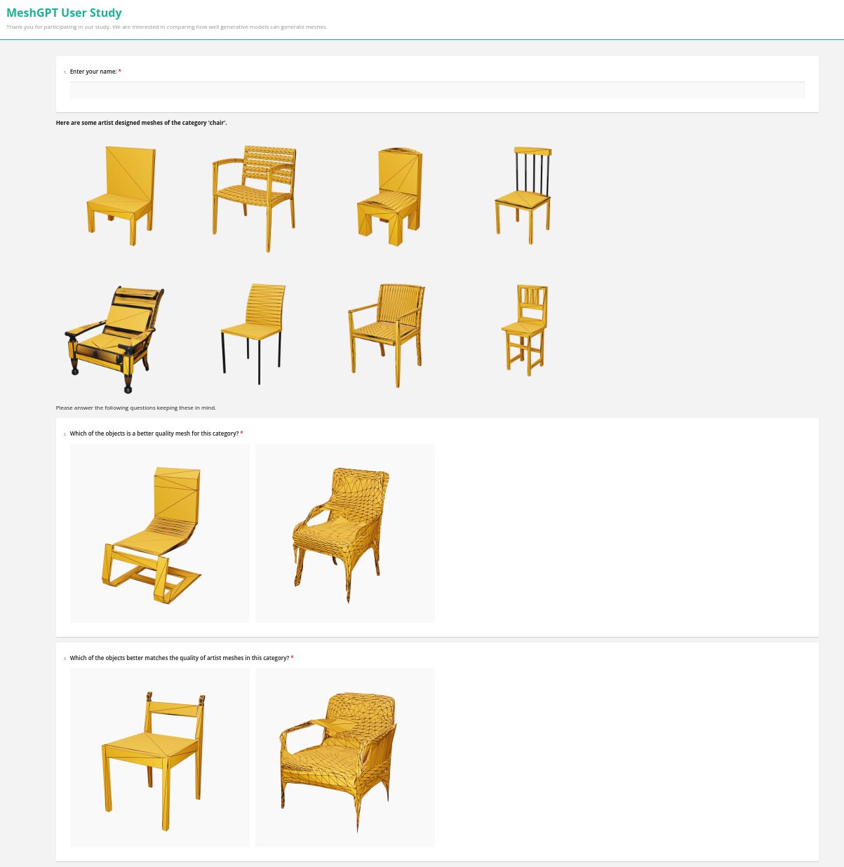
We develop a Django-based web application for the user study. In Fig. 15, we show the interface for the questionnaire. We randomly select 16 pairs of meshes from each baseline and our method across the Chair and Table categories, half of which are used for a question on preference based on shape quality, and the other half for preference based on triangulation quality. After the samples are prepared, we ask the users to pick the sample which they prefer more based on the question. To avoid biases in this user study, we shuffle the pairs so that there is no positional hint to our method. We also show a collection of ground-truth meshes to the user for them to get an idea of the real distribution. In the end, we gather 784 responses from 49 participants to calculate the preferences.

Appendix D Shape Novelty Analysis

Fig. 12 and 13 displays the top-3 most similar shapes from the train set corresponding to all samples used in the main paper that were generated by our model. These nearest neighbor shapes are identified based on Chamfer Distance (CD). To ensure a fair distance computation, accounting for potential discrepancies due to scale or shift in the augmented generations, we normalize all generated and train shapes to be centered within $[0,1]^{3}$ and scaled to the extremes of this cube.

Appendix E Additional Results

Metrics. Following recent works for unconditional shape generation Yu et al. 2022; Zeng et al. 2022; Erkoç et al. 2023 for calculating the shape metrics we define

$$\text{MMD}(S_{g},S_{r}) =\frac{1}{|S_{r}|}\sum_{Y\in S_{r}}\min_{X\in S_{g}}D(X,Y),$$

$$\text{COV}(S_{g},S_{r}) =\frac{|\{\operatornamewithlimits{argmin}_{Y\in S_{r}}D(X,Y)|X\in S_{g}\}|}{|S_{r}|},$$

$$\text{1-NNA}(S_{g},S_{r}) =\frac{\sum_{X\in S_{g}}\mathbbm{1}_{X}+\sum_{Y\in S_{r}}\mathbbm{1}_{Y}}{|S_{g}|+|S_{r}|},$$

$$\mathbbm{1}_{X} =\mathbbm{1}[N_{X}\in S_{g}],$$

$$\mathbbm{1}_{Y} =\mathbbm{1}[N_{Y}\in S_{r}],$$

where in the 1-NNA metric $N_{X}$ is a point cloud that is closest to $X$ in both generated and reference dataset, i.e.,

$$N_{X}=\operatornamewithlimits{argmin}_{K\in S_{r}\cup S_{g}}D(X,K)$$

We use a Chamfer Distance (CD) distance measure $D(X,Y)$ for computing these metrics in 3D. To evaluate these point-based measures, we sample $2048$ points randomly from all baseline outputs; and use $6000$, $1200$, $1000$, $8000$ generated shapes from chair, bench, lamp and table categories.

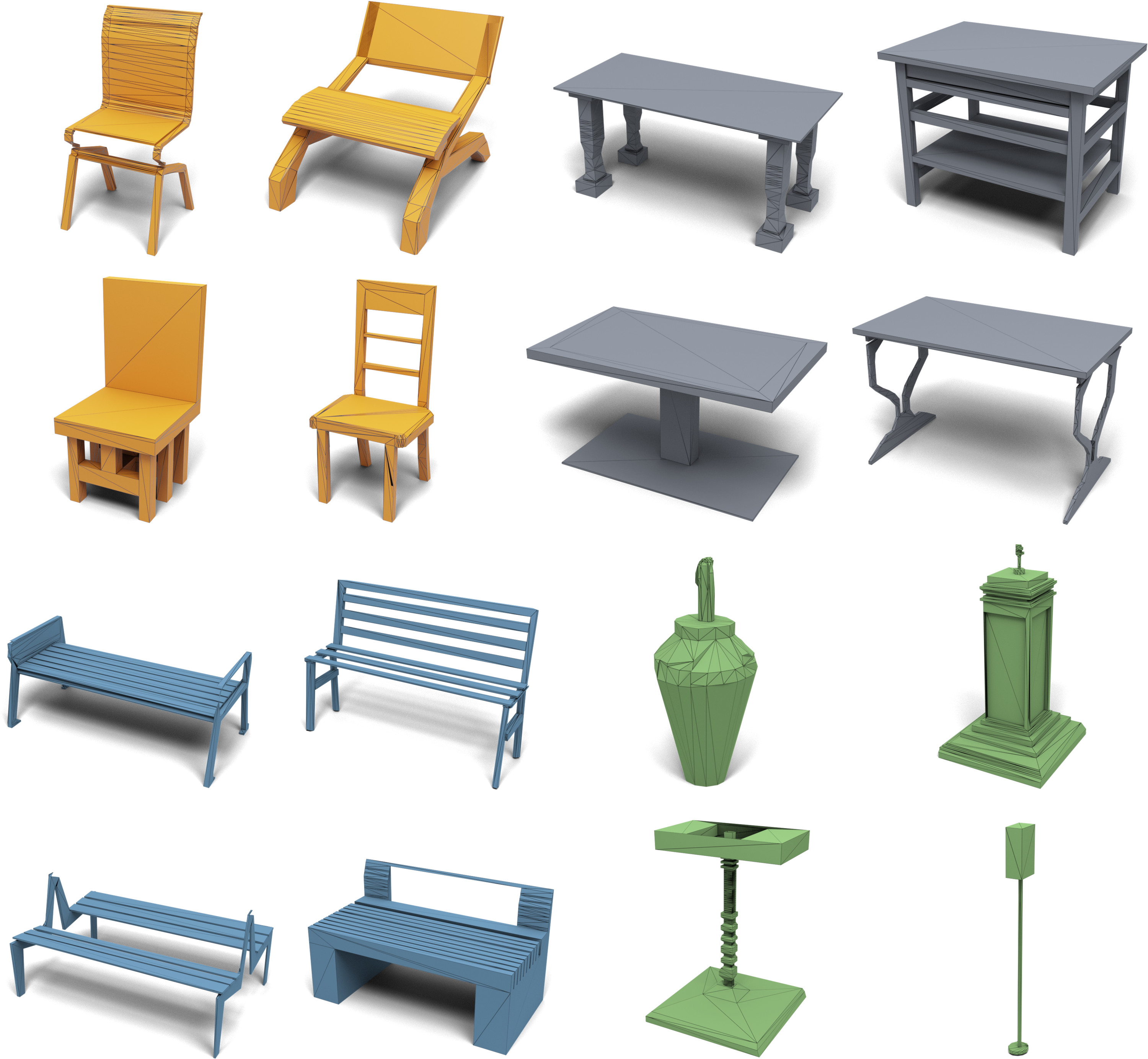
Qualitative Results. Fig. 11 shows more unconditional generations from our model across different ShapeNet categories.

Variant	Triangle Accuracy (%) $\uparrow$	Cross-Entropy $\downarrow$
w/o Positional Encoding	79.33	0.2484
w/o Output Discretization	22.03	0.5705
w/o Residual Quantization	1.29	4.6679
w/o per Vertex Quantization	98.64	0.1413
w/ PointNet Encoder	88.73	0.1896
w/ GAT Veličković et al. 2017 Encoder	86.14	0.2015
w/ EdgeConv Wang et al. 2019 Encoder	91.23	0.1702
w/ ResNet19 Decoder	96.29	0.1492
w/ PointNet Decoder	95.47	0.1528
MeshGPT	98.49	0.1473

Table 4: Ablations of our design choices for the encoder-decoder network on the Chair category of the ShapeNet Chang et al. 2015 dataset.

Encoder-Decoder Ablations. In Tab. 4, we show a set of ablations on the design choice for our encoder-decoder network used for learning the triangle embeddings. We measure the performance in terms of triangle accuracy, which measures average accuracy with which all 9 coordinates of faces are correctly predicted, and the cross-entropy loss on the test set.

Figure 16: The effectiveness of per-vertex quantization over per-face quantization can be understood through an example where two faces share an edge as shown above. With per-face tokenization assigning 6 tokens per face, the sequence yields 12 unique tokens. In contrast, per-vertex tokenization leads to repeated tokens in the sequence due to shared vertices between faces. This repetition makes the sequence easier for the transformer to learn compared to a wholly unique sequence per face, especially when both sequences are of equal length.

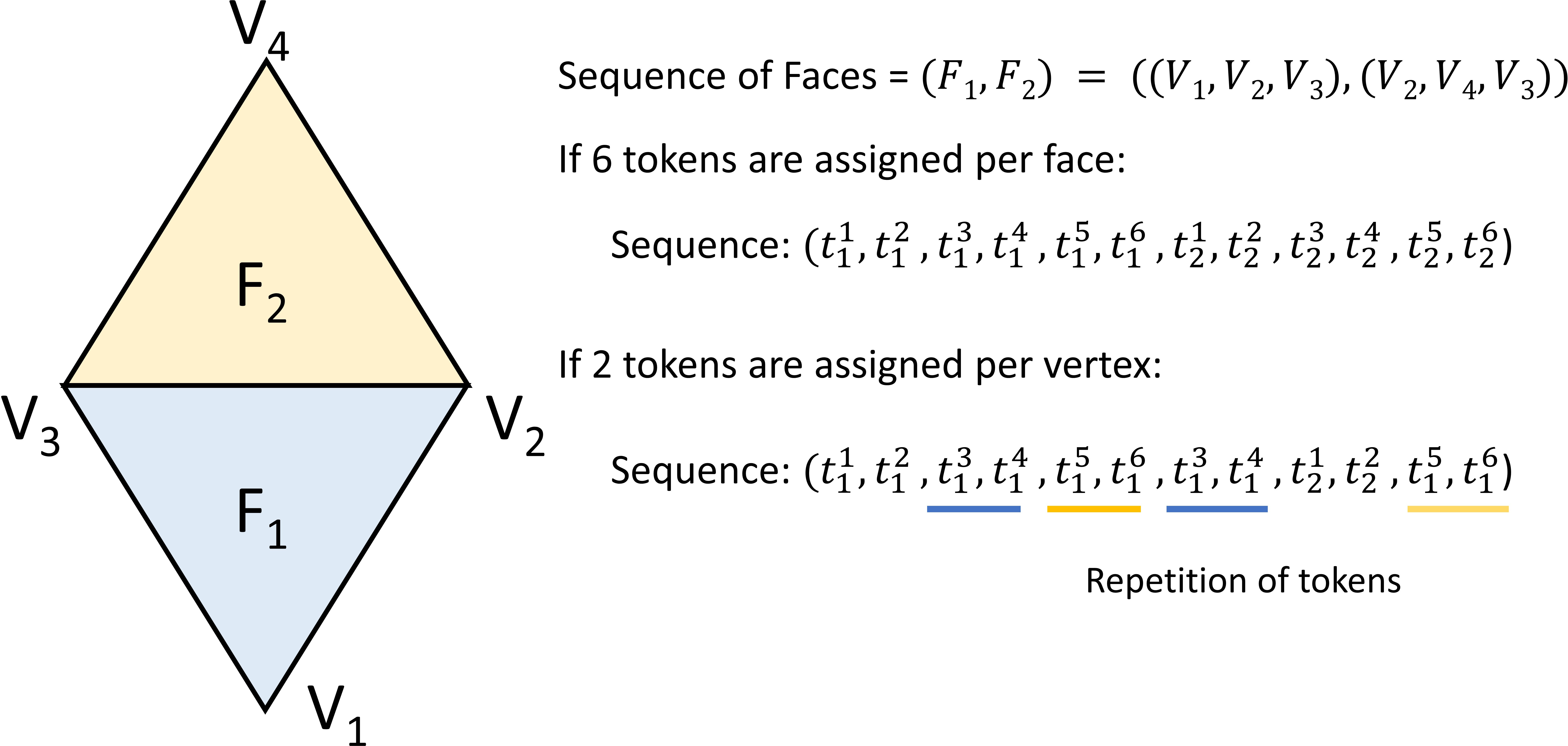
We evaluate the effect of various choices – how much does the positional encoding at input help, effect of using continuous predictions instead of discrete as outputs, using vector quantization (1 token per face) instead of residual quantization ($D$ tokens per face), encoder architecture as a point encoder, or different graph convolution operators, and decoder architecture as either ResNet19 or PointNet decoder. Note that even though for encoder-decoder reconstruction, ‘w/o per Vertex Quantization’ performs best, this variant works significantly worse than with per Vertex Quantization, as shown in the main paper. Fig. 16 describes an intuition of why the embeddings from this variant are more transformer friendly.

References

- Achlioptas et al. [2018] Panos Achlioptas, Olga Diamanti, Ioannis Mitliagkas, and Leonidas Guibas. Learning representations and generative models for 3d point clouds. In International conference on machine learning, pages 40–49. PMLR, 2018.
- Blumberg [1920] Henry Blumberg. Hausdorff’s grundzüge der mengenlehre. 1920.
- Brock et al. [2016] Andrew Brock, Theodore Lim, James M Ritchie, and Nick Weston. Generative and discriminative voxel modeling with convolutional neural networks. arXiv preprint arXiv:1608.04236, 2016.
- Cai et al. [2020] Ruojin Cai, Guandao Yang, Hadar Averbuch-Elor, Zekun Hao, Serge Belongie, Noah Snavely, and Bharath Hariharan. Learning gradient fields for shape generation. In Computer Vision–ECCV 2020: 16th European Conference, Glasgow, UK, August 23–28, 2020, Proceedings, Part III 16, pages 364–381. Springer, 2020.
- Chang et al. [2015] Angel X. Chang, Thomas Funkhouser, Leonidas Guibas, Pat Hanrahan, Qixing Huang, Zimo Li, Silvio Savarese, Manolis Savva, Shuran Song, Hao Su, Jianxiong Xiao, Li Yi, and Fisher Yu. ShapeNet: An Information-Rich 3D Model Repository. Technical Report arXiv:1512.03012 [cs.GR], Stanford University — Princeton University — Toyota Technological Institute at Chicago, 2015.
- Chen and Zhang [2019] Zhiqin Chen and Hao Zhang. Learning implicit fields for generative shape modeling. In Proceedings of the IEEE/CVF Conference on Computer Vision and Pattern Recognition, pages 5939–5948, 2019.
- Chen et al. [2020] Zhiqin Chen, Andrea Tagliasacchi, and Hao Zhang. Bsp-net: Generating compact meshes via binary space partitioning. In Proceedings of the IEEE/CVF Conference on Computer Vision and Pattern Recognition, pages 45–54, 2020.
- Cheng et al. [2023] Yen-Chi Cheng, Hsin-Ying Lee, Sergey Tulyakov, Alexander G Schwing, and Liang-Yan Gui. Sdfusion: Multimodal 3d shape completion, reconstruction, and generation. In Proceedings of the IEEE/CVF Conference on Computer Vision and Pattern Recognition, pages 4456–4465, 2023.
- Choy et al. [2016] Christopher B Choy, Danfei Xu, JunYoung Gwak, Kevin Chen, and Silvio Savarese. 3d-r2n2: A unified approach for single and multi-view 3d object reconstruction. In Computer Vision–ECCV 2016: 14th European Conference, Amsterdam, The Netherlands, October 11-14, 2016, Proceedings, Part VIII 14, pages 628–644. Springer, 2016.
- Community [2018] Blender Online Community. Blender - a 3D modelling and rendering package. Blender Foundation, Stichting Blender Foundation, Amsterdam, 2018.
- Dai and Nießner [2019] Angela Dai and Matthias Nießner. Scan2mesh: From unstructured range scans to 3d meshes. In Proceedings of the IEEE/CVF Conference on Computer Vision and Pattern Recognition, pages 5574–5583, 2019.
- Doi and Koide [1991] Akio Doi and Akio Koide. An efficient method of triangulating equi-valued surfaces by using tetrahedral cells. IEICE TRANSACTIONS on Information and Systems, 74(1):214–224, 1991.
- Erkoç et al. [2023] Ziya Erkoç, Fangchang Ma, Qi Shan, Matthias Nießner, and Angela Dai. Hyperdiffusion: Generating implicit neural fields with weight-space diffusion. arXiv preprint arXiv:2303.17015, 2023.
- Gao et al. [2022] Jun Gao, Tianchang Shen, Zian Wang, Wenzheng Chen, Kangxue Yin, Daiqing Li, Or Litany, Zan Gojcic, and Sanja Fidler. Get3d: A generative model of high quality 3d textured shapes learned from images. Advances In Neural Information Processing Systems, 35:31841–31854, 2022.
- Garland and Heckbert [1997] Michael Garland and Paul S Heckbert. Surface simplification using quadric error metrics. In Proceedings of the 24th annual conference on Computer graphics and interactive techniques, pages 209–216, 1997.
- Gong et al. [2019] Shunwang Gong, Lei Chen, Michael Bronstein, and Stefanos Zafeiriou. Spiralnet++: A fast and highly efficient mesh convolution operator. In Proceedings of the IEEE/CVF international conference on computer vision workshops, pages 0–0, 2019.
- Goodfellow et al. [2020] Ian Goodfellow, Jean Pouget-Abadie, Mehdi Mirza, Bing Xu, David Warde-Farley, Sherjil Ozair, Aaron Courville, and Yoshua Bengio. Generative adversarial networks. Communications of the ACM, 63(11):139–144, 2020.
- Groueix et al. [2018] Thibault Groueix, Matthew Fisher, Vladimir G Kim, Bryan C Russell, and Mathieu Aubry. A papier-mâché approach to learning 3d surface generation. In Proceedings of the IEEE conference on computer vision and pattern recognition, pages 216–224, 2018.
- Gupta et al. [2023] Anchit Gupta, Wenhan Xiong, Yixin Nie, Ian Jones, and Barlas Oğuz. 3dgen: Triplane latent diffusion for textured mesh generation. arXiv preprint arXiv:2303.05371, 2023.
- Hamilton et al. [2017] Will Hamilton, Zhitao Ying, and Jure Leskovec. Inductive representation learning on large graphs. Advances in neural information processing systems, 30, 2017.
- Hanocka et al. [2019] Rana Hanocka, Amir Hertz, Noa Fish, Raja Giryes, Shachar Fleishman, and Daniel Cohen-Or. Meshcnn: a network with an edge. ACM Transactions on Graphics (ToG), 38(4):1–12, 2019.
- He et al. [2016] Kaiming He, Xiangyu Zhang, Shaoqing Ren, and Jian Sun. Deep residual learning for image recognition. In Proceedings of the IEEE conference on computer vision and pattern recognition, pages 770–778, 2016.
- Hu et al. [2022] Shi-Min Hu, Zheng-Ning Liu, Meng-Hao Guo, Jun-Xiong Cai, Jiahui Huang, Tai-Jiang Mu, and Ralph R Martin. Subdivision-based mesh convolution networks. ACM Transactions on Graphics (TOG), 41(3):1–16, 2022.
- Hui et al. [2022] Ka-Hei Hui, Ruihui Li, Jingyu Hu, and Chi-Wing Fu. Neural wavelet-domain diffusion for 3d shape generation. In SIGGRAPH Asia 2022 Conference Papers, pages 1–9, 2022.
- Jain et al. [2022] Ajay Jain, Ben Mildenhall, Jonathan T Barron, Pieter Abbeel, and Ben Poole. Zero-shot text-guided object generation with dream fields. In Proceedings of the IEEE/CVF Conference on Computer Vision and Pattern Recognition, pages 867–876, 2022.
- Jimenez Rezende et al. [2016] Danilo Jimenez Rezende, SM Eslami, Shakir Mohamed, Peter Battaglia, Max Jaderberg, and Nicolas Heess. Unsupervised learning of 3d structure from images. Advances in neural information processing systems, 29, 2016.
- Juang and Gray [1982] Biing-Hwang Juang and A Gray. Multiple stage vector quantization for speech coding. In ICASSP’82. IEEE International Conference on Acoustics, Speech, and Signal Processing, pages 597–600. IEEE, 1982.
- Kingma and Ba [2014] Diederik P Kingma and Jimmy Ba. Adam: A method for stochastic optimization. arXiv preprint arXiv:1412.6980, 2014.
- Lee et al. [2022] Doyup Lee, Chiheon Kim, Saehoon Kim, Minsu Cho, and Wook-Shin Han. Autoregressive image generation using residual quantization. In Proceedings of the IEEE/CVF Conference on Computer Vision and Pattern Recognition, pages 11523–11532, 2022.
- Li et al. [2018] Chun-Liang Li, Manzil Zaheer, Yang Zhang, Barnabas Poczos, and Ruslan Salakhutdinov. Point cloud gan. arXiv preprint arXiv:1810.05795, 2018.
- Li et al. [2023] Muheng Li, Yueqi Duan, Jie Zhou, and Jiwen Lu. Diffusion-sdf: Text-to-shape via voxelized diffusion. In Proceedings of the IEEE/CVF Conference on Computer Vision and Pattern Recognition, pages 12642–12651, 2023.
- Liao et al. [2018] Yiyi Liao, Simon Donne, and Andreas Geiger. Deep marching cubes: Learning explicit surface representations. In Proceedings of the IEEE Conference on Computer Vision and Pattern Recognition, pages 2916–2925, 2018.
- Lim et al. [2018] Isaak Lim, Alexander Dielen, Marcel Campen, and Leif Kobbelt. A simple approach to intrinsic correspondence learning on unstructured 3d meshes. In Proceedings of the European Conference on Computer Vision (ECCV) Workshops, pages 0–0, 2018.
- Lin et al. [2023] Chen-Hsuan Lin, Jun Gao, Luming Tang, Towaki Takikawa, Xiaohui Zeng, Xun Huang, Karsten Kreis, Sanja Fidler, Ming-Yu Liu, and Tsung-Yi Lin. Magic3d: High-resolution text-to-3d content creation. In Proceedings of the IEEE/CVF Conference on Computer Vision and Pattern Recognition, pages 300–309, 2023.
- Liu et al. [2023] Zhen Liu, Yao Feng, Michael J Black, Derek Nowrouzezahrai, Liam Paull, and Weiyang Liu. Meshdiffusion: Score-based generative 3d mesh modeling. arXiv preprint arXiv:2303.08133, 2023.
- Lorensen and Cline [1998] William E Lorensen and Harvey E Cline. Marching cubes: A high resolution 3d surface construction algorithm. In Seminal graphics: pioneering efforts that shaped the field, pages 347–353. 1998.
- Luo and Hu [2021] Shitong Luo and Wei Hu. Diffusion probabilistic models for 3d point cloud generation. In Proceedings of the IEEE/CVF Conference on Computer Vision and Pattern Recognition, pages 2837–2845, 2021.
- Martinez et al. [2014] Julieta Martinez, Holger H Hoos, and James J Little. Stacked quantizers for compositional vector compression. arXiv preprint arXiv:1411.2173, 2014.
- Mescheder et al. [2019] Lars Mescheder, Michael Oechsle, Michael Niemeyer, Sebastian Nowozin, and Andreas Geiger. Occupancy networks: Learning 3d reconstruction in function space. In Proceedings of the IEEE/CVF conference on computer vision and pattern recognition, pages 4460–4470, 2019.
- Milano et al. [2020] Francesco Milano, Antonio Loquercio, Antoni Rosinol, Davide Scaramuzza, and Luca Carlone. Primal-dual mesh convolutional neural networks. Advances in Neural Information Processing Systems, 33:952–963, 2020.
- Müller et al. [2023] Norman Müller, Yawar Siddiqui, Lorenzo Porzi, Samuel Rota Bulo, Peter Kontschieder, and Matthias Nießner. Diffrf: Rendering-guided 3d radiance field diffusion. In Proceedings of the IEEE/CVF Conference on Computer Vision and Pattern Recognition, pages 4328–4338, 2023.
- Nan and Wonka [2017] Liangliang Nan and Peter Wonka. Polyfit: Polygonal surface reconstruction from point clouds. In Proceedings of the IEEE International Conference on Computer Vision, pages 2353–2361, 2017.
- Nash et al. [2020] Charlie Nash, Yaroslav Ganin, SM Ali Eslami, and Peter Battaglia. Polygen: An autoregressive generative model of 3d meshes. In International conference on machine learning, pages 7220–7229. PMLR, 2020.
- Nichol et al. [2022] Alex Nichol, Heewoo Jun, Prafulla Dhariwal, Pamela Mishkin, and Mark Chen. Point-e: A system for generating 3d point clouds from complex prompts. arXiv preprint arXiv:2212.08751, 2022.
- Park et al. [2019] Jeong Joon Park, Peter Florence, Julian Straub, Richard Newcombe, and Steven Lovegrove. Deepsdf: Learning continuous signed distance functions for shape representation. In Proceedings of the IEEE/CVF conference on computer vision and pattern recognition, pages 165–174, 2019.
- Paszke et al. [2019] Adam Paszke, Sam Gross, Francisco Massa, Adam Lerer, James Bradbury, Gregory Chanan, Trevor Killeen, Zeming Lin, Natalia Gimelshein, Luca Antiga, Alban Desmaison, Andreas Kopf, Edward Yang, Zachary DeVito, Martin Raison, Alykhan Tejani, Sasank Chilamkurthy, Benoit Steiner, Lu Fang, Junjie Bai, and Soumith Chintala. Pytorch: An imperative style, high-performance deep learning library. In Advances in Neural Information Processing Systems 32, pages 8024–8035. Curran Associates, Inc., 2019.
- Peng et al. [2021] Songyou Peng, Chiyu Jiang, Yiyi Liao, Michael Niemeyer, Marc Pollefeys, and Andreas Geiger. Shape as points: A differentiable poisson solver. Advances in Neural Information Processing Systems, 34:13032–13044, 2021.
- Poole et al. [2022] Ben Poole, Ajay Jain, Jonathan T Barron, and Ben Mildenhall. Dreamfusion: Text-to-3d using 2d diffusion. arXiv preprint arXiv:2209.14988, 2022.
- Remelli et al. [2020] Edoardo Remelli, Artem Lukoianov, Stephan Richter, Benoit Guillard, Timur Bagautdinov, Pierre Baque, and Pascal Fua. Meshsdf: Differentiable iso-surface extraction. Advances in Neural Information Processing Systems, 33:22468–22478, 2020.
- Schwarz et al. [2022] Katja Schwarz, Axel Sauer, Michael Niemeyer, Yiyi Liao, and Andreas Geiger. Voxgraf: Fast 3d-aware image synthesis with sparse voxel grids. Advances in Neural Information Processing Systems, 35:33999–34011, 2022.
- Sharp and Ovsjanikov [2020] Nicholas Sharp and Maks Ovsjanikov. Pointtrinet: Learned triangulation of 3d point sets. In Computer Vision–ECCV 2020: 16th European Conference, Glasgow, UK, August 23–28, 2020, Proceedings, Part XXIII 16, pages 762–778. Springer, 2020.
- Sharp et al. [2022] Nicholas Sharp, Souhaib Attaiki, Keenan Crane, and Maks Ovsjanikov. Diffusionnet: Discretization agnostic learning on surfaces. ACM Transactions on Graphics (TOG), 41(3):1–16, 2022.
- Shen et al. [2021] Tianchang Shen, Jun Gao, Kangxue Yin, Ming-Yu Liu, and Sanja Fidler. Deep marching tetrahedra: a hybrid representation for high-resolution 3d shape synthesis. Advances in Neural Information Processing Systems, 34:6087–6101, 2021.
- Shu et al. [2019] Dong Wook Shu, Sung Woo Park, and Junseok Kwon. 3d point cloud generative adversarial network based on tree structured graph convolutions. In Proceedings of the IEEE/CVF international conference on computer vision, pages 3859–3868, 2019.
- Shue et al. [2023] J Ryan Shue, Eric Ryan Chan, Ryan Po, Zachary Ankner, Jiajun Wu, and Gordon Wetzstein. 3d neural field generation using triplane diffusion. In Proceedings of the IEEE/CVF Conference on Computer Vision and Pattern Recognition, pages 20875–20886, 2023.
- Smirnov and Solomon [2021] Dmitriy Smirnov and Justin Solomon. Hodgenet: Learning spectral geometry on triangle meshes. ACM Transactions on Graphics (TOG), 40(4):1–11, 2021.
- Tatarchenko et al. [2017] Maxim Tatarchenko, Alexey Dosovitskiy, and Thomas Brox. Octree generating networks: Efficient convolutional architectures for high-resolution 3d outputs. In Proceedings of the IEEE international conference on computer vision, pages 2088–2096, 2017.
- Touvron et al. [2023] Hugo Touvron, Louis Martin, Kevin Stone, Peter Albert, Amjad Almahairi, Yasmine Babaei, Nikolay Bashlykov, Soumya Batra, Prajjwal Bhargava, Shruti Bhosale, et al. Llama 2: Open foundation and fine-tuned chat models. arXiv preprint arXiv:2307.09288, 2023.
- Valsesia et al. [2018] Diego Valsesia, Giulia Fracastoro, and Enrico Magli. Learning localized generative models for 3d point clouds via graph convolution. In International conference on learning representations, 2018.
- Veličković et al. [2017] Petar Veličković, Guillem Cucurull, Arantxa Casanova, Adriana Romero, Pietro Lio, and Yoshua Bengio. Graph attention networks. arXiv preprint arXiv:1710.10903, 2017.
- Wang et al. [2019] Yue Wang, Yongbin Sun, Ziwei Liu, Sanjay E Sarma, Michael M Bronstein, and Justin M Solomon. Dynamic graph cnn for learning on point clouds. ACM Transactions on Graphics (tog), 38(5):1–12, 2019.
- Wu et al. [2016] Jiajun Wu, Chengkai Zhang, Tianfan Xue, Bill Freeman, and Josh Tenenbaum. Learning a probabilistic latent space of object shapes via 3d generative-adversarial modeling. Advances in neural information processing systems, 29, 2016.
- Xu et al. [2023] Jiale Xu, Xintao Wang, Weihao Cheng, Yan-Pei Cao, Ying Shan, Xiaohu Qie, and Shenghua Gao. Dream3d: Zero-shot text-to-3d synthesis using 3d shape prior and text-to-image diffusion models. In Proceedings of the IEEE/CVF Conference on Computer Vision and Pattern Recognition, pages 20908–20918, 2023.
- Yang et al. [2019] Guandao Yang, Xun Huang, Zekun Hao, Ming-Yu Liu, Serge Belongie, and Bharath Hariharan. Pointflow: 3d point cloud generation with continuous normalizing flows. In Proceedings of the IEEE/CVF international conference on computer vision, pages 4541–4550, 2019.
- Yang et al. [2018] Yaoqing Yang, Chen Feng, Yiru Shen, and Dong Tian. Foldingnet: Point cloud auto-encoder via deep grid deformation. In Proceedings of the IEEE conference on computer vision and pattern recognition, pages 206–215, 2018.
- Yu et al. [2022] Xumin Yu, Lulu Tang, Yongming Rao, Tiejun Huang, Jie Zhou, and Jiwen Lu. Point-bert: Pre-training 3d point cloud transformers with masked point modeling. In Proceedings of the IEEE/CVF Conference on Computer Vision and Pattern Recognition, pages 19313–19322, 2022.
- Zeng et al. [2022] Xiaohui Zeng, Arash Vahdat, Francis Williams, Zan Gojcic, Or Litany, Sanja Fidler, and Karsten Kreis. Lion: Latent point diffusion models for 3d shape generation. In Advances in Neural Information Processing Systems, 2022.
- Zhou et al. [2021] Linqi Zhou, Yilun Du, and Jiajun Wu. 3d shape generation and completion through point-voxel diffusion. In Proceedings of the IEEE/CVF International Conference on Computer Vision, pages 5826–5835, 2021.