Learning Coarse Propagators in Parareal Algorithms

Abstract

The parareal algorithm represents an important class of parallel-in-time algorithms for solving evolution equations and has been widely applied in practice. To achieve effective speedup, the choice of the coarse propagator in the algorithm is vital. In this work, we investigate the use of learned coarse propagators. Building upon the error estimation framework, we present a systematic procedure for constructing coarse propagators that enjoy desirable stability and consistent order. Additionally, we provide preliminary mathematical guarantees for the resulting parareal algorithm. Numerical experiments on a variety of settings, e.g., linear diffusion model, Allen-Cahn model, and viscous Burgers model, show that learning can significantly improve parallel efficiency when compared with the more ad hoc choice of some conventional and widely used coarse propagators.

1 Introduction

This paper is devoted to accelerating a class of parareal solvers for parabolic problems using machine learning techniques. Let $T>0$ be a fixed terminal time. Consider the following initial value problem for $u\in C((0,T];D({\mathcal{A}}))\cap C([0,T];{\mathcal{H}})$:

(1) $$\left\{\begin{aligned} &u^{\prime}(t)+{\mathcal{A}}u(t)=f(t),\quad 0<t<T,\\ &u(0)=u^{0},\end{aligned}\right.$$

where $u^{0}\in{\mathcal{H}}$ is the initial data, $f:[0,T]\to{\mathcal{H}}$ is a given forcing term, and ${\mathcal{A}}$ is a positive definite, self-adjoint, linear operator with a compact inverse, defined over a Hilbert space $({\mathcal{H}},(\cdot,\cdot))$ (with the induced norm $\|\cdot\|$) with its domain $D({\mathcal{A}})$ dense in ${\mathcal{H}}$. This model arises in a very broad range of practical applications, and its effective numerical simulation is of enormous importance and has received a lot of attention [36].

The numerical solution of the model (1) commonly employs time discretization, and various time-stepping schemes have been proposed; see the monograph [36] for an in-depth treatment. Typically these schemes proceed step by step, and the process is sequential in nature. This represents the major bottleneck in the numerical solution of the model (1), especially for large time. In the ground-breaking work [27], Lions, Maday and Turinici proposed the so-called parareal algorithm for solving evolution models in a parallel-in-time manner. The method has been established as a fundamental tool to utilize highly parallel systems when distributed computing in space saturates. Since its inception, this class of methods have been applied successfully to numerous diverse practical applications, e.g., option pricing [5, 33], multiscale kinetics [12, 3], stochastic PDEs [8] and fractional diffusion [39, 26].

The parareal algorithm is based on two solvers, one coarse propagator (CP), of low accuracy but fast enough to be applied sequentially, and one fine propagator (FP) with full accuracy, applied in parallel in time. At each iteration, the CP is run sequentially over each subdomain, and then the FP is run in parallel as a correction. See Section 2.2 for the details on how the CP and FP interact. The CP is usually based on one or a few steps of a standard numerical solver, and in practice, it is often a numerical integrator using lower resolution, e.g., much larger time step size, in order to effectively propagate the information forward in time. Ideally, the parareal algorithm can achieve the accuracy of the FP at the efficiency of the CP. The choice of the CP is crucial to achieve the desired speedup on modern multicore / many-core computer architectures. Nonetheless, the optimal choice of CP remains highly nontrivial. Even worse, for the model (1) with nonsmooth data, the convergence of the parareal algorithm with the standard backward Euler CP is somehow limited [37, 30, 13, 41], which essentially restricts the achievable efficiency, cf. (5) below for the precise statement. This issue occurs with other commonly used CPs [13, Tables 1 and 2]. These observations naturally lead to the interesting question whether it is possible to overcome the convergence barrier of parareal algorithm by properly modifying the CP.

In this work we propose an innovative and easy-to-implement framework for designing CPs in parareal algorithms for problem (1). It builds on the error estimation framework [16, 35, 13, 41], and follows the prevalent paradigm of using learning to address challenges in scientific computing. Specifically, based on an analytic convergence factor derived in the error estimation framework, we construct a learned coarse propagator (LCP) to minimize an upper bound on the convergence factor. In this way, the LCP is specifically learned for the underlying FP, which differs markedly from the conventional choice where the CP is almost agnostic to the choice of the FP. We provide a systematic procedure for constructing CPs that respect highly desirable properties, e.g., stability and accuracy. We present a preliminary analysis of the framework, which shows that LCPs can indeed achieve the desired goal for linear evolution problems. Several numerical experiments on linear and nonlinear problems, including linear diffusion model, Allen-Cahn model and viscous Burgers equation, are presented to illustrate the approach. The numerical results show that employing learning techniques consistently enhances performance compared to the conventional choice of using the backward Euler scheme (or other popular single step methods) as the CP.

Broadly, this work follows the prevalent paradigm of learning numerical algorithms for scientific computing, which combines mathematically driven, handcrafted design of general algorithm structure with a data-driven adaptation to specific classes of tasks [6, 19, 31, 20, 23, 24]. For example, Guo et al [20] present a machine learning approach that automatically learns effective solvers for initial value problems in the form of ordinary differential equations, based on the Runge-Kutta integrator, and learn high-order integrators for targeted families of differential equations. The use of LCPs in designing new parareal algorithms has also been explored [40, 1, 32, 24]. Yalla and Engquist [40] explored the use of neural networks approximating the phase map as a CP for high-dimensional harmonic oscillators and localized multiscale problems. Agboh et al [1] used a feed-forward deep neural network as a CP to integrate an ODE, and observed improved performance. Nguyen and Tsai [32] used supervised learning to enhance its efficiency for wave propagation. Ibrahim et al [24] proposed to use a physics-informed neural network (PINN) as a CP, and show the speedup on the Black-Scholes equation which performs better than a numerical CP. The present work continues along this active line of research on enhancing parareal algorithms with learning concept [40, 1, 32, 24], but with the major difference of explicitly building analytic insights into the learning procedure, i.e., stability and consistency, and consequently the learned CPs proposed in this work enjoy rigorous mathematical guarantees.

The rest of the paper is organized as follows. In Section 2, we recall preliminary materials on single step time stepping methods and parareal algorithm. In Section 3 we develop learned coarse propagators, and analyze their properties. Then in Section 4 we illustrate the performance of trained coarse propagators on several model problems.

2 Single step methods and parareal algorithm

First we describe the abstract framework of single step time stepping methods for solving problem (1), and give a brief overview of the parareal algorithm. For an in-depth treatment of these topics, we refer interested readers to the monograph [36] and the review [14].

2.1 Single step solvers for parabolic equations

To discretize problem (1) in time, we divide the time interval $(0,T)$ into $N$ equidistant subintervals, each of length ${\Delta t}=T/N$, and let the grid points be $t_{n}=n{\Delta t}$, for $n=0,1,\ldots,N$. Then a single step scheme approximates the solution $u(t_{n+1})$ by

(2) $$u^{n+1}=r({\Delta t}{\mathcal{A}})u^{n}+{\Delta t}\sum_{i=1}^{m}p_{i}({\Delta t}{\mathcal{A}})f(t_{n}+c_{i}\Delta t),\quad\text{for}~{}0\leq n\leq N-1.$$

Here $r(\lambda)$ and the sequence $\{p_{i}(\lambda)\}^{m}_{i=1}$ are rational functions, and ${c_{i}}$ are distinct real numbers in $[0,1]$. Below we impose the following conditions on the scheme (2):

• $|r(\lambda)|<1$ and $|p_{i}(\lambda)|\leq c$, for all $i=1,\ldots,m$, for any ${\Delta t}$ and for any $\lambda>0$. Further, the numerator of $p_{i}(\lambda)$ is of strictly lower degree than the denominator.

• The scheme (2) is accurate of order $q$ in the sense that

  $$r(\lambda)=e^{-\lambda}+\mathcal{O}(\lambda^{q+1}),\quad\text{as}~{}\lambda\rightarrow 0.$$

  Additionally, for every $0\leq j\leq q$,

  $$\sum_{i=1}^{m}c_{i}^{j}p_{i}(\lambda)-\frac{j!}{(-\lambda)^{j+1}}\Big{(}e^{-\lambda}-\sum_{\ell=0}^{j}\frac{(-\lambda)^{\ell}}{\ell!}\Big{)}=\mathcal{O}(\lambda^{q-j}),\quad\text{as}~{}\lambda\rightarrow 0.$$

• The rational function $r(\lambda)$ is strongly stable in the sense that $|r(\infty)|<1$.

See, e.g., the monograph [36, p. 131] for the construction of rational functions satisfying properties (P1)-(P3). (P3) is crucial for ensuring the convergence of parareal iteration, for especially nonsmooth problem data (e.g., $u^{0}\in\mathcal{H}$). When $|r(\infty)|=1$ (e.g., Crank-Nicolson and implicit Runge-Kutta of Gauss type), the convergence of the parareal method depends on two factors. First, the eigenvalues of ${\mathcal{A}}$ must be bounded from above, which is typically not the case for parabolic equations. Second, the ratio between the coarse and fine step sizes must be sufficiently large, with the precise value determined by the upper bound of the eigenvalues of ${\mathcal{A}}$. Schemes not satisfying (P3) may lose the optimal convergence rate [36, Chapter 8].

In practice, it is often desirable to choose $p_{i}(\lambda)$ sharing the denominator with $r(\lambda)$, i.e., for polynomials $a_{i}(\lambda)$ and $g(\lambda)$ such that

$$r(\lambda)=\frac{a_{0}(\lambda)}{g(\lambda)}\quad\text{and}\quad p_{i}(\lambda)=\frac{a_{i}(\lambda)}{g(\lambda)},\quad\text{for}~{}i=1,2,\ldots,m.$$

Then the scheme (2) can be written as

$$g({\Delta t}{\mathcal{A}})u^{n+1}=a_{0}({\Delta t}{\mathcal{A}})u^{n}+{\Delta t}\sum_{i=1}^{m}a_{i}({\Delta t}{\mathcal{A}})f(t_{n}+c_{i}\Delta t),\quad\text{for}~{}1\leq n\leq N-1.$$

The following error estimate holds for the scheme (2) [36, Theorems 7.2 and 8.1].

Lemma 2.1.

Let conditions (P1)-(P3) be fulfilled, $u(t)$ the solution to problem (1), and $u^{n}$ the solution to the scheme (2). Then there holds

$$\|u^{n}-u(t_{n})\|\leq c\,(\Delta t)^{q}\Big{(}t_{n}^{-q}\|u^{0}\|+t_{n}\sum_{\ell=0}^{q-1}\sup_{s\leq t_{n}}\|{\mathcal{A}}^{q-\ell}f^{(\ell)}(s)\|+\int_{0}^{t_{n}}\|f^{(q)}(s)\|\,{\mathrm{d}}s\Big{)},$$

if $u_{0}\in{\mathcal{H}}$, $f^{(\ell)}\in C([0,T];\mathrm{Dom}({\mathcal{A}}^{q-\ell})$ with $0\leq\ell\leq q-1$ and $f^{(q)}\in L^{1}(0,T;{\mathcal{H}})$.

Remark 2.2.

By Lemma 2.1, under conditions (P1)-(P3), the solution $u^{n}$ of the scheme (2) converges to the exact one $u(t_{n})$ at an order $\mathcal{O}((\Delta t)^{q})$, if $f$ and $u_{0}$ fulfill certain compatibility conditions. For example, when ${\mathcal{A}}=-\Delta$, equipped with a zero Dirichlet boundary condition, the requirement is $(-\Delta)^{\ell}f^{(q-\ell)}=0$ on $\partial\Omega$ for $0\leq\ell\leq q$. To circumvent these stringent conditions, the scheme (2) is assumed to be strictly accurate of order $q$ such that

$$\sum_{i=1}^{m}c_{i}^{j}p_{i}(\lambda)-\frac{j!}{(-\lambda)^{j+1}}\Big{(}r(\lambda)-\sum_{\ell=0}^{j}\frac{(-\lambda)^{\ell}}{\ell!}\Big{)}=0,\quad\text{for}~{}0\leq j\leq q-1.$$

A scheme is strictly accurate of order $p_{0}<p$ if the truncation error vanishes for all $f$ and $u_{0}$ such that the solution is a polynomial in $t$ of degree at most $p_{0}-1$. While a single step method with a given $m\in\mathbb{N}$ might be accurate to order $2m$ (e.g., Gauss–Legendre method) [11, Section 2.2], it can be strictly accurate of order only up to order $m+1$ [9, Lemma 5].

Remark 2.3.

The error estimate in Lemma 2.1 can be improved if the integrator exhibits L-stability, i.e., $r(\infty)=0$ [36, Theorem 7.2].

2.2 Parareal algorithm

Now we present the parareal algorithm for the single step integrator (2). Let $\Delta T=J\Delta t$ be the coarse step size, $N_{c}=T/\Delta T\in\mathbb{N}$, and denote $T_{n}=n\Delta T$. The numerical propagators ${\mathcal{G}}$ and ${\mathcal{F}}$ correspond to the coarse and fine time grids, respectively. Typically, ${\mathcal{G}}$ is an inexpensive, low-order numerical method (e.g., backward Euler scheme), whereas ${\mathcal{F}}$ is defined by the single step integrator (2). For any given initial data $v\in{\mathcal{H}}$ and $f\in C([0,T];{\mathcal{H}})$, the coarse and fine propagators are respectively defined by

(3) $${\mathcal{G}}(T_{n},\Delta T,v,f) =R({\Delta T}{\mathcal{A}})v+{\Delta T}\sum_{i=1}^{M}P_{i}({\Delta T}{\mathcal{A}})f(T_{n}+C_{i}\Delta T),$$

(4) $${\mathcal{F}}(t_{n},\Delta t,v,f) =r({\Delta t}{\mathcal{A}})v+{\Delta t}\sum_{i=1}^{m}p_{i}({\Delta t}{\mathcal{A}})f(t_{n}+c_{i}\Delta t),$$

where $M$ and $m$ denote the numbers of stages of the CP $\mathcal{G}$ and FP $\mathcal{F}$, respectively, and $R$ and $P$ are rational functions for the CP $\mathcal{G}$, and $r$ and $p$ for the FP $\mathcal{F}$. The parareal iteration is given in Algorithm 1.

Algorithm 1 Parareal algorithm.

1:  Initialization: Compute $U_{0}^{n+1}={\mathcal{G}}(T_{n},\Delta T,U_{0}^{n+1},f)$ with $U_{0}^{0}=u^{0}$, $n=0,1,...,N_{c}-1$;

2:  for $k=0,1,\ldots,K$ do

3:     On each subinterval $[T_{n},T_{n+1}]$, sequentially compute for $j=0,1,2,\dots,J-1$

$$\widetilde{U}^{n,j+1}_{k}={\mathcal{F}}(T_{n}+j\Delta t,\Delta t,\widetilde{U}^{n,j}_{k},f),$$

with initial value $\widetilde{U}^{n,0}_{k}=U_{k}^{n}$, and set $\widetilde{U}^{n+1}_{k}=\widetilde{U}^{n,J}_{k}$.

4:     Perform sequential corrections, i.e., find $U_{k+1}^{n+1}$ by

$$U_{k+1}^{n+1}={\mathcal{G}}(T_{n},\Delta T,U_{k+1}^{n},f)+\widetilde{U}^{n+1}_{k}-{\mathcal{G}}(T_{n},\Delta T,U_{k}^{n},f)$$

with $U_{k+1}^{0}=u^{0}$, for $n=0,1,...,N_{c}-1$;

5:     Check the stopping criterion.

6:  end for

The convergence of parallel algorithms has been extensively studied (see, e.g., [4, 8, 16, 30, 37, 38, 13, 41] for a rather incomplete list). Very recently, for linear evolution equations, Yang, Yuan and Zhou [41] proved that with the backward Euler scheme as the CP, there exists a threshold $J_{*}>0$, independent of $\Delta T$, $\Delta t$ and the upper bound of the spectrum of ${\mathcal{A}}$, such that under conditions (P1)-(P3), if $J\geq J_{*}$, then the following bound holds with $\gamma\approx 0.3$,

(5) $$\max_{1\leq n\leq N_{c}}\|U_{k}^{n}-u^{nJ}\|\leq c\,\gamma^{k},$$

where $U_{k}^{n}$ denotes the parareal solution, and $u^{nJ}$ the fine time stepping solution. Numerically the estimate (5) is observed to be sharp. This issue arises with other types of CPs; the work [13] reported an optimal mesh-independent convergence factor $\gamma\approx 0.26$ when both CP and FP are the two-stage, second-order singly diagonally implicit Runge Kutta scheme (SDIRK-22), and $\gamma\approx 0.15$ when both are SDIRK-33, for $J\in\{4,8,16,32,64\}$. These observations naturally motivate the following question: Are there alternative CPs capable of overcoming these barriers, significantly improving convergence, while maintaining robustness across different $J$ values? Below we aim at learning new CPs to accelerate the convergence of the parareal algorithm.

3 Learning coarse propagators

Now we develop a systematic strategy to construct CPs, termed as learned CP (LCP), which yields a Learned CP (LCP) achieving a convergence factor $\gamma\approx 0.02$ when $J\in[16,128]$ for linear evolution problems, thereby overcoming the barrier (5) on the convergence rate. We also discuss basic properties of the resulting parareal algorithm.

3.1 Error estimation

Now we present the error estimation framework in the work [16, 41] by incorporating a general coarse/fine propagator. See also a tighter convergence bound in [35, Theorem 30]. Consider the coarse and fine propagators defined in (3)–(4), which both satisfy conditions (P1)-(P3). For the difference between the solution $U_{k+1}^{n+1}$ by the parareal time stepping scheme and the fine grid solution $u^{(n+1)J}$, we deduce

$$U_{k+1}^{n+1}-u^{(n+1)J} =R(\Delta T{\mathcal{A}})\Big{[}(U_{k+1}^{n}-u^{nJ})-(U_{k}^{n}-u^{nJ})\Big{]}$$

$$\quad+{\mathcal{F}}(T_{n}+(J-1)\Delta t,\Delta t,\widetilde{U}^{n,J-1}_{k},f)-{\mathcal{F}}(T_{n}+(J-1)\Delta t,\Delta t,u^{(n+1)J-1},f)$$

$$=R(\Delta T{\mathcal{A}})\Big{[}(U_{k+1}^{n}-u^{nJ})-(U_{k}^{n}-u^{nJ})\Big{]}+r(\Delta t{\mathcal{A}})(\widetilde{U}^{n,J-1}_{k}-u^{(n+1)J-1})$$

$$=R(\Delta T{\mathcal{A}})\Big{[}(U_{k+1}^{n}-u^{nJ})-(U_{k}^{n}-u^{nJ})\Big{]}+r(\Delta t{\mathcal{A}})^{J}(\widetilde{U}^{n,0}_{k}-u^{nJ})$$

$$=R(\Delta T{\mathcal{A}})\Big{[}(U_{k+1}^{n}-u^{nJ})-(U_{k}^{n}-u^{nJ})\Big{]}+r(\Delta t{\mathcal{A}})^{J}(U_{k}^{n}-u^{nJ}).$$

Upon letting $E_{k}^{n}=U_{k}^{n}-u^{nJ}$, we can rewrite the identity by

$$E_{k+1}^{n+1}=R(\Delta T{\mathcal{A}})(E_{k+1}^{n}-E_{k}^{n})+r(\Delta tA)^{J}E_{k}^{n}.$$

Recall that the linear operator ${\mathcal{A}}$ is positive definite and selfadjoint with a compact inverse on Hilbert space $({\mathcal{H}},(\cdot,\cdot))$. By the spectral theory for compact operators [42], ${\mathcal{A}}$ has positive eigenvalues $\{\lambda_{j}\}_{j=1}^{\infty}$, where $0<\lambda_{1}\leq\lambda_{2}\leq\ldots$ and $\lambda_{j}\rightarrow\infty$, and the corresponding eigenfunctions $\{\phi_{j}\}_{j=1}^{\infty}$ form an orthonormal basis of the Hilbert space ${\mathcal{H}}$. Then, with $e_{k,j}^{n}=(E_{k}^{n},\phi_{j})$, by means of spectral decomposition, we derive

$$e_{k+1,j}^{n+1}=R(\Delta T\lambda_{j})(e_{k+1,j}^{n}-e_{k,j}^{n})+r(\Delta t\lambda_{j})^{J}e_{k,j}^{n}.$$

Upon setting $d_{j}=\Delta T\lambda_{j}$, we get

$$e_{k+1,j}^{n+1}=R(d_{j})e_{k+1,j}^{n}+(r(d_{j}/J)^{J}-R(d_{j}))e_{k,j}^{n}.$$

Applying the recursion repeatedly and noting the condition $e_{k+1,j}^{0}=0$ yield

$$e_{k+1,j}^{n+1} =(r(d_{j}/J)^{J}-R(d_{j}))e_{k,j}^{n}+R(d_{j})e_{k+1,j}^{n}$$

$$=(r(d_{j}/J)^{J}-R(d_{j}))(e_{k,j}^{n}+R(d_{j})e_{k,j}^{n-1})+R(d_{j})^{2}e_{k+1,j}^{n-1}$$

$$=(r(d_{j}/J)^{J}-R(d_{j}))(e_{k,j}^{n}+R(d_{j})e_{k,j}^{n-1}+\dots+R(d_{j})^{n-1}e_{k,j}^{1}).$$

Now, taking the absolute value on both sides gives

$$|e_{k+1,j}^{n+1}| \leq|r(d_{j}/J)^{J}-R(d_{j})|\cdot(1+|R(d_{j})|+\dots+|R(d_{j})|^{n-1})\max_{1\leq n\leq N_{c}-1}{|e_{k,j}^{n}|}$$

$$\leq\frac{|r(d_{j}/J)^{J}-R(d_{j})|}{1-|R(d_{j})|}\max_{1\leq n\leq N_{c}-1}{|e_{k,j}^{n}|}$$

(6) $$\leq\sup_{s\in\{\Delta T\lambda_{j}\}_{j=1}^{\infty}}\frac{|r(s/J)^{J}-R(s)|}{1-|R(s)|}\max_{1\leq n\leq N_{c}-1}{|e_{k,j}^{n}|}.$$

This inequality naturally suggests the following componentwise convergence factor

$$\kappa(r,R,J,s)=\frac{r(s/J)^{J}-R(s)}{1-|R(s)|},$$

and likewise the convergence factor for $J_{0}$

(7) $$\kappa_{c}(r,R;J_{0})=\sup_{s\in\Lambda}|\kappa(r,R,J_{0},s)|,\quad\mbox{with }\Lambda=\{\Delta T\lambda_{j}\}_{j=1}^{\infty}.$$

The next result shows that $\kappa_{c}(r,R;J_{0})$ determines the convergence of the parareal method: If $\kappa_{c}(r,R;J_{0})<1$, then $\max_{1\leq n\leq N_{c}}\|E_{k}^{n}\|\to 0$ as $k\rightarrow\infty$. That is, the solution $U_{k}^{n}$ by the parareal algorithm converges to the fine time stepping solution $u^{nJ}$ as $k\rightarrow\infty$.

Theorem 3.1.

Let conditions (P1)-(P3) be fulfilled and the data regularity assumption in Lemma 2.1 hold. Let $u^{n}$ be the solution by the FP (4), and $U^{n}_{k}$ the solution by Algorithm 1. Then the following error estimate holds

$$\max_{1\leq n\leq N_{c}}\|U^{n}_{k}-u^{nJ}\|\leq c\kappa_{c}(r,R;J)^{k}.$$

Proof 3.2.

In Algorithm 1, the initial guess $U_{0}^{n}$ is obtained by the coarse propagator $\mathcal{G}$. Then Lemma 2.1 (with $q\geq 1$) implies

(8) $$\|U_{0}^{n}-u^{nJ}\| \leq\|U_{0}^{n}-u(T_{n})\|+\|u(T_{n})-u^{nJ}\|\leq cn^{-1}.$$

With $E_{k}^{n}=U_{k}^{n}-u^{nJ}$ and $e_{k,j}^{n}=(E_{k}^{n},\phi_{j})$, then the relation (3.1) implies

$$\max_{1\leq n\leq N_{c}}\|E_{k}^{n}\|^{2} \leq\sum_{j=1}^{\infty}\max_{1\leq n\leq N_{c}}|e_{k,j}^{n}|^{2}\leq{\kappa_{c}(r,R;J)}^{2}\sum_{j=1}^{\infty}\max_{1\leq n\leq N_{c}}|e_{k-1,j}^{n}|^{2}$$

$$\leq\cdots\leq\kappa_{c}(r,R;J)^{2k}\sum_{j=1}^{\infty}\max_{1\leq n\leq N_{c}}|e_{0,j}^{n}|^{2}.$$

This and the inequality $\max_{1\leq n\leq N_{c}}|e_{0,j}^{n}|^{2}\leq\sum_{n=1}^{N_{c}}|e_{0,j}^{n}|^{2}$ yield

$$\max_{1\leq n\leq N_{c}}\|E_{k}^{n}\|^{2} \leq c\kappa_{c}(r,R;J)^{2k}\sum_{j=1}^{\infty}\sum_{n=1}^{N_{c}}|e_{0,j}^{n}|^{2}\leq c\kappa_{c}(r,R;J)^{2k}\sum_{n=1}^{N_{c}}\|E_{0}^{n}\|^{2}$$

$$\leq c^{2}\kappa_{c}(r,R;J)^{2k}\sum_{n=1}^{N_{c}}n^{-2}\leq c^{2}\kappa_{c}(r,R;J)^{2k},$$

where the second last inequality is due to the estimate (8).

3.2 Learning coarse propagator

Given a high-order single step scheme as the FP $\mathcal{F}$, we shall learn a CP to expedite the convergence of parareal iteration. We consider a parametric stability function $R(\lambda,\bm{\theta})$ in terms of $\lambda$, defined by

(9) $$R(\lambda,\bm{\theta})=\frac{P_{n}(\lambda,\bm{\theta})}{Q_{m}(\lambda,\bm{\theta})}=\frac{\sum^{n}_{i=0}a_{i}\lambda^{i}}{1+\sum^{m}_{i=1}e^{b_{i}}\lambda^{i}}.$$

The parameters is grouped as $\bm{\theta}=(b_{1},...,b_{q},b_{q+1},...,b_{m},a_{q+1},...,a_{n})$ and $\bm{\theta}^{\prime}=(a_{0},...,a_{q})$, with $q<n\leq m$. Note that $\bm{\theta}^{\prime}$ is excluded from $\bm{\theta}$. We discuss this exclusion and the parameter $q$ below. The exponential representation in the denominator of $R(\lambda,\theta)$ is to enhance the training stability. For any optimal $\bm{\theta}^{*}$, according to conditions (P1)-(P3), ideally, the learned stability function $R(\lambda,\bm{\theta}^{*})$ in (9) of the LCP $\mathcal{G}_{\bm{\theta}^{*}}$ should satisfy

1. (P1), (P3): The LCP $\mathcal{G}_{\bm{\theta}^{*}}$ is stable and strongly stable, i.e.,

   $$|R(\lambda,\bm{\theta}^{*})|<1~{}\text{for}~{}\lambda>0~{}\text{and}~{}|R(\infty,\bm{\theta}^{*})|<1.$$

2. (P2): The LCP $\mathcal{G}_{\bm{\theta}^{*}}$ has an accuracy of order $q$, i.e., $R(\lambda,\bm{\theta}^{*})=e^{-\lambda}+\mathcal{O}(\lambda^{q+1})$.

Inspired by these requirements, we define the error function $e(\lambda,\bm{\theta}^{*})$ by

$$e(\lambda,\bm{\theta}^{*})=e^{-\lambda}-R(\lambda,\bm{\theta}^{*})=e^{-\lambda}-\frac{P_{n}(\lambda,\bm{\theta}^{*})}{Q_{m}(\lambda,\bm{\theta}^{*})},$$

and let $E(\lambda,\bm{\theta}^{*})\coloneqq e(\lambda,\bm{\theta}^{*})Q_{m}(\lambda,\bm{\theta}^{*})=e^{-\lambda}Q_{m}(\lambda,\bm{\theta}^{*})-P_{n}(\lambda,\bm{\theta}^{*})$. Given $q\leq n$, in order to ensure having enough trainable parameters, we request $E^{(k)}(0,\bm{\theta}^{*})=0,\ k=0,1,...,q$, i.e.,

$$\frac{{\rm d}^{k}}{{\rm d}\lambda^{k}}(e^{-\lambda}Q_{m})(0,\bm{\theta}^{*})=\frac{{\rm d}^{k}}{{\rm d}\lambda^{k}}P_{n}(0,\bm{\theta}^{*}),\quad k=0,1,\cdot\cdot\cdot,q.$$

By Taylor expansion, with $e^{-\lambda}=\sum^{\infty}_{i=0}c_{i}\lambda^{i}$, we obtain

(10) $$\sum^{k}_{j=0}c_{j}e^{b_{k-j}}=a_{k},\quad k=0,1,\cdot\cdot\cdot,q.$$

That is, the parameter vector $\bm{\theta}^{\prime}$ is fully determined by $(b_{1},\ldots,b_{q})$, one block of $\bm{\theta}$, under the given consistency constraint. In practice, it is not learned, and we use the identity (10) to determine $\bm{\theta}^{\prime}$ directly (i.e., $\bm{\theta}^{\prime}=\bm{\theta}^{\prime}(\bm{\theta})$), and learn only the parameters $\bm{\theta}$.

The learned stability function $R(\lambda,\bm{\theta})$ is chosen to minimize the convergence factor $\kappa_{c}(r,R;J_{0})$. However, it is inconvenient to compute $\Lambda$ since $\lambda_{j}\rightarrow\infty$. So we approximate the operator ${\mathcal{A}}$ with a matrix $A_{h}$ [36, Section 1], and approximate $\Lambda$ in (7) with $\Lambda_{h}$ (associated with $A_{h}$). This requires deriving upper and lower eigenvalue bounds of $A_{h}$, e.g., using Rayleigh quotient [18]. To approximate the set $\Lambda_{h}$, we sample uniformly over the eigenvalue range of $\Lambda_{h}$.

Now consider the learning of a CP $\mathcal{G}_{\bm{\theta}}$. Given the stability function $r(\lambda)$ of the FP $\mathcal{F}$, we select the parameters $m$, $n$, $q$, $J_{0}$ and $N_{1}$. The resulting optimization problem reads

(11) $$\underset{\bm{\theta}}{\text{min}}\ \kappa_{c}(r,R; J_{0})\quad\text{s.t.}\quad\sum^{k}_{j=0}c_{j}e^{b_{k-j}}=a_{k},\,k=0,1,\dots,q,\,\mbox{and}\,|R(\lambda,\bm{\theta})|<1,~{}\lambda>0.$$

These constraints enforce properties (P1)–(P3), i.e., stability and convergence order. The construction naturally respects highly desirable features of an ideal CP.

To strictly enforce the condition $|R(\lambda,\bm{\theta})|<1$ for $\lambda>0$, we define a set $\Lambda_{R}$ (with a cardinality $N_{R}$), which encompasses all positive critical points of $R(s,\bm{\theta})$ and the limit of $R(s,\bm{\theta})$ as $s\rightarrow\infty$. Since the stability function $R(s,\bm{\theta})$ is known, computing $\Lambda_{R}$ a priori is feasible for a fixed $\bm{\theta}$. Then it suffices to verify the condition $|R(\lambda,\bm{\theta})|<1$ for $\lambda\in\Lambda_{R}$. We adopt the barrier method [28, Chapter 13], in order to strictly enforce the condition:

(12) $$\mathcal{L}_{\rm b}(\bm{\theta})=\frac{1}{N_{R}}\sum_{s\in\Lambda_{R}}\log(1-R^{2}(s,\bm{\theta})).$$

Then the total loss $\mathcal{L}_{\rho}$ is given by

(13) $$\mathcal{L}_{\rho}(\bm{\theta})=\mathcal{L}_{\rm s}(\bm{\theta})-\rho\mathcal{L}_{\rm b}(\bm{\theta}),\quad\mbox{with }\mathcal{L}_{\rm s}(\bm{\theta})=\sup_{s\in\Lambda_{h}}\frac{|r(s/J_{0})^{J_{0}}-R(s,\bm{\theta})|}{1-|R(s,\bm{\theta})|},$$

where $\rho>0$ is the weight for the barrier function. To ensure the convergence of the barrier method to problem (11) during training, we choose the weight $\rho$ by a path-following strategy: we initialize with $\rho_{0}$, and then geometrically decrease its value, i.e., $\rho_{i+1}=\beta\rho_{i}$, for some $\beta\in(0,1)$. Let $\theta_{k}^{*}$ be a minimizer of the loss $\mathcal{L}_{\rho_{k}}(\theta)$. Then any limit point of the sequence $\{\bm{\theta}_{k}^{*}\}$ solves problem (11) [28, Chapter 13]. The complete procedure for learning the CP $\mathcal{G}_{\bm{\theta}}$ is given in Algorithm 2. To minimize the loss $\mathcal{L}_{\rho}$, we employ subgradient descent; see [17, 7, 34, 25] for relevant convergence analysis.

Algorithm 2 Learning the CP for the FP $\mathcal{F}$.

1:  Specify parameters $m,n,q,J_{0},N_{1},$ $\rho_{0}$, $\beta$, and initialize $\bm{\theta}$ randomly.

2:  Compute the set $\Lambda_{h}$.

3:  for $i=0,1,\ldots$ do

4:     $\rho_{i+1}=\beta\rho_{i}.$

5:     for $k=0,1,\ldots,K$ do

6:        Given $\bm{\theta}$, find the set $\Lambda_{R}$.

7:        Construct the loss $\mathcal{L}_{\rho_{i}}(\bm{\theta})=\mathcal{L}_{\rm s}(\bm{\theta})-\rho_{i}\cdot\mathcal{L}_{\rm b}(\bm{\theta})$

8:        Minimize the loss $\mathcal{L}_{\rho_{i}}(\bm{\theta})$ and update $\bm{\theta}$.

9:        Check the stopping criterion.

10:     end for

11:     Check the stopping criterion.

12:  end for

13:  return  $\bm{\theta}$.

Next we compute $P_{i}(\lambda,\bm{\theta})$, and request that the LCP is strictly accurate of order $q$:

(14) $$\sum_{i=1}^{m}C_{i}^{j}P_{i}(\lambda,\bm{\theta})-\frac{j!}{(-\lambda)^{j+1}}\Big{(}R(\lambda,\bm{\theta})-\sum_{\ell=0}^{j}\frac{(\lambda)^{\ell}}{\ell!}\Big{)}=0,\quad\forall 0\leq j\leq q-1.$$

We employ a uniform distribution for the values of $C_{i}^{j}$ within the interval $[0,1]$, so as to solve $P_{i}(\lambda,\bm{\theta})$ via linear systems. When $i=1$, we take $C_{i}^{j}=1$ in order to have the better stability of a backward scheme. Finally, $R(\lambda,\bm{\theta})$ and $P_{i}(\lambda,\bm{\theta})$ together define the LCP:

$${\mathcal{G}}(T_{n},\Delta T,v,f)=R({\Delta T}A,\bm{\theta})v+{\Delta T}\sum_{i=1}^{M_{1}}P_{i}({\Delta T}A,\bm{\theta})f(T_{n}+C_{i}\Delta T).$$

In practice, we take two, three, four-stage Lobatto IIIC method and three-stage Radau IIA method [21, 22] as the FP $\mathcal{F}$, and give the learned $R(\lambda,\bm{\theta})$ in Appendix A.

Proposition 3.3.

For any optimal choice of the parameter $\bm{\theta}$, the LCP is consistent and has an accuracy of order $q$. Furthermore, it is strongly stable.

Proof 3.4.

Note that we learn the LCP according to conditions (P1)-(P3). First, the LCP satisfies condition (P2) and equation (14), so it is consistent, with at least an accuracy of order $q$. Second, due to the presence of the penalty term $\mathcal{L}_{\rm b}(\bm{\theta})$ (12), the LCP satisfies both conditions (P1) and (P3), implying its strong stability.

3.3 Robustness with respect to $J$

In Algorithm 2, the ratio $J_{0}$ of the coarse step size $\Delta T$ to the fine one $\Delta t$ is predetermined for learning the parameters. It is important to study the robustness of the algorithm with respect to the choice of $J$. The next result shows that the convergence factor remains stable in $J$. To this end, we study the supremum of $\kappa(r,R,J,s)$ over the interval $\mathbb{R}_{+}:=(0,\infty)$: $\kappa_{c}(r,R;J)\leq\sup_{s\in\mathbb{R}_{+}}|\kappa(r,R,J,s)|$. The convexity assumption $g^{\prime\prime}(J)\geq 0$ on $g(J)=r(s/J)^{J}$ with respect to $J$ (for $s>0$) holds for two and four-stage Lobatto IIIC methods, and three-stage Radau IIA method. In practice, the ratio $J$ is important: a too small $J$ leads to big and non-negligible cost, whereas a too large $J$ requires more outer loops. Hence, we have chosen $J\in[16,128]$ in the analysis below.

Theorem 3.5.

Let $J_{1},J_{2}\in[16,128]$ such that $\ J_{1}\leq J_{2}$. Let $r(s)$ be the stability function of the FP, satisfying (i) conditions (P1)-(P3); (ii) $g^{\prime\prime}(J)>0$, with $g(J)=r(s/J)^{J}$ for any given $s\in\mathbb{R}_{+}$; and (iii) $r(s)\geq 0$, for any $s\in\mathbb{R}_{+}$. Let $R(s,\bm{\theta})$ be the stability function of the LCP. Then there holds

$$\sup_{s\in\mathbb{R}_{+}}|\kappa(r,R,J_{2},s)|-\sup_{s\in\mathbb{R}_{+}}|\kappa(r,R,J_{1},s)|\leq 112\sup_{s\in\mathbb{R}_{+}}|h(s)|,$$

with the function $h(s)$ given by

(15) $$h(s)=\frac{r(s)^{15}}{1-|R(16s,\bm{\theta})|}\cdot(r(s)\ln r(s)-r^{\prime}(s)s).$$

Proof 3.6.

By definition, for any $s^{*}\in\mathbb{R}_{+}$, we have

$$|\kappa(r,R,J_{2},s^{*})|-\sup_{s\in\mathbb{R}_{+}}|\kappa(r,R,J_{1},s)|$$

$$\leq |\kappa(r,R,J_{2},s^{*})|-|\kappa(r,R,J_{1},s^{*})|\leq|\kappa(r,R,J_{2},s^{*})-\kappa(r,R,J_{1},s^{*})|.$$

We claim that for any $J\in[16,128]$ and $s>0$

(16) $$\frac{\rm d}{{\rm d}J}\kappa(r,R,J,s)\leq 0\quad\text{and}\quad\frac{{\rm d}^{2}}{{\rm d}J^{2}}\kappa(r,R,J,s)\geq 0.$$

Now with $g(J)$, we have $\kappa(r,R,J,s)=\frac{g(J)-R(s,\bm{\theta})}{1-|R(s,\bm{\theta})|}$. Since $|R(s,\bm{\theta})|<1$ for $s>0$ (and independent of $J$), it suffices to prove $g^{\prime}(J)\leq 0$ and $g^{\prime\prime}(J)\geq 0$ for $J\in[16,128]$ and $s>0$. Let $f(J):=\ln g(J)=J\ln r(s/J)$. Then we have

(17) $$g^{\prime}(J)=f^{\prime}(J)g(J)\quad\mbox{and}\quad g^{\prime\prime}(J)=\frac{f^{\prime\prime}(J)g(J)^{2}+(g^{\prime}(J))^{2}}{g(J)}.$$

The first two derivatives of $f(J)$ in $J$ are given by

(18) $$f^{\prime}(J) =\ln r({s}/{J})-\frac{s}{r(s/J)}\frac{r^{\prime}(s/J)}{J}\quad\mbox{and}\quad f^{\prime\prime}(J) =\frac{r^{\prime\prime}(s/J)r(s/J)-(r^{\prime}(s/J))^{2}}{r(s/J)^{2}J^{3}}s^{2}.$$

Clearly, $r(0)=1$ and $r^{\prime}(0)=-1$, so we have $f^{\prime}(\infty)=0$. By assumption (ii), we have $g^{\prime\prime}(J)\geq 0$, and $g^{\prime}(\infty)=0$. These facts imply $g^{\prime}(J)\leq 0$, yielding the estimates in (16). Since $\kappa(r,R,J,s_{2})$ is twice differentiable in $J$ over the interval $[16,128]$, we obtain

$$|\kappa(r,R,J_{2},s^{*})-\kappa(r,R,J_{1},s^{*})|\leq\sup_{J\in[16,128]}\Big{|}\frac{\rm d}{{\rm d}J}\kappa(r,R,J,s^{*})\Big{|}(J_{2}-J_{1})$$

$$\leq \Big{|}\frac{\rm d}{{\rm d}J}\kappa(r,R,16,s^{*})\Big{|}(128-16)=112\sup_{s\in\mathbb{R}_{+}}\Big{|}\frac{\rm d}{{\rm d}J}\kappa(r,R,16,16s)\Big{|}.$$

Then noting the identity $h(s)=\frac{{\mathrm{d}}}{{\mathrm{d}}J}\kappa(r,R,16,16s)=\frac{r(s)^{15}}{1-|R(16s,\bm{\theta})|}\cdot(r(s)\ln r(s)-r^{\prime}(s)s)$, and taking the supremum over all $s\in\mathbb{R}_{+}$ complete the proof.

The next result discusses the robustness of the LCP for the two-stage Lobatto IIIC method.

Corollary 3.7.

The two-stage Lobatto IIIC method satisfies the assumptions in Theorem 3.5, and $|h(s)|\leq\text{4.91e-4}$. Further, for $J_{1},J_{2}\in[16,128]$ with $J_{1}\leq J_{2}$, we have

$$\sup_{s_{2}\in\mathbb{R}_{+}}|\kappa(r,R,J_{2},s_{2})|-\sup_{s_{1}\in\mathbb{R}_{+}}|\kappa(r,R,J_{1},s_{1})|\leq 0.055.$$

Proof 3.8.

For the two-stage Lobatto IIIC method, we have $r(s)=\frac{2}{s^{2}+2s+2}$. We claim that $r(s)$ satisfies the assumptions in Theorem 3.5. Indeed, Assumptions (i) and (iii) hold trivially. To see Assumption (ii), we write $r(s)={P_{r}(s)}/{Q_{r}(s)}$ and employ equations (17) and (18). We claim the following inequality

(19) $$r^{\prime\prime}(s)r(s)\geq(r^{\prime}(s))^{2},\quad\forall s\in\mathbb{R}_{+},$$

or equivalently,

$$\frac{P_{r}(s)P^{\prime\prime}_{r}(s)-(P^{\prime}_{r}(s))^{2}}{P_{r}(s)^{2}}\geq\frac{Q_{r}(s)Q^{\prime\prime}_{r}(s)-(Q^{\prime}_{r}(s))^{2}}{Q_{r}(s)^{2}},\quad\forall s\in\mathbb{R}_{+},$$

which can be verified directly using the explicit form of $r(s)$. For the two-stage Lobatto IIIC method, the stability function $R(s,\bm{\theta})$ of the LCP is given by (cf. Appendix A)

$$R(s,\bm{\theta})=\frac{{1.0-0.20967s+0.00484s^{2}}}{{1.0+0.79033s+0.37931s^{2}}},$$

For the function $h$ defined in (15), we claim $|h(s)|\leq\text{4.91e-4}$ for $s>0$. We divide the proof of the desired assertion into the following three steps: (i) $h(s)\leq 0$ for $s>0$; (ii) bound $h$ for $s\in[1/2,\infty)$, i.e., $h(s)>\text{-2.1e-4}$ for $s\in[1/2,\infty)$; and (iii) bound $h$ for $s\in(0,1/2)$, i.e., $h(s)\geq 0.506\cdot(\text{-9.5e-4})\geq\text{-4.91e-4}$.
Step (i): Let $\varphi(s)=\ln r(s)-\frac{r^{\prime}(s)s}{r(s)}$. From the inequality (19), we deduce $\varphi^{\prime}(s)=\frac{s((r^{\prime}(s))^{2}-r^{\prime\prime}(s)r(s))}{r^{2}(s)}\leq 0$. Then we derive $\varphi(s)\leq\varphi(0^{+})=0$, which implies $h(s)\leq h(0^{+})\leq 0$.
Step (ii): For $s\in[1/2,\infty)$, we have

$$\frac{\rm d}{{\rm d}s}R(s,\bm{\theta})\approx\frac{1.0-0.74894s+0.083355s^{2}}{(1.0+0.79033s+0.37931s^{2})^{2}}.$$

Thus $R(16s,\bm{\theta})$ has a unique extremum at $\bar{s}\approx 0.6353$, and $R(16s,\bm{\theta})$ is decreasing on $[1/2,\bar{s}]$ and increasing on $(\bar{s},\infty)$. Hence, $|R(16s,\bm{\theta})|\leq\max\{|R(16\bar{s},\bm{\theta})|,|R(\infty,\bm{\theta})|\}\leq\text{1.4e-2}$, and

$$h(s)\geq\frac{r(s)^{16}\ln r(s)}{1-|R(16s,\bm{\theta})|}\geq 1.015\cdot r(s)^{16}\ln r(s):=\psi(s).$$

Clearly, $\psi^{\prime}(s)=1.015r(s)^{15}r^{\prime}(s)(16\ln r(s)+r(s))$, and also $r>0$ and $r^{\prime}<0$, from which it follows directly that $\psi^{\prime}(s)>0$ for $s>1/2$. Hence, we deduce $h(s)\geq\psi(s)\geq\psi(1/2)>\text{-2.1e-4}$.
Step (iii): For $s\in(0,1/2]$, note that there exists a unique root $s^{\ast}\approx 0.341$ of $R(16s^{\ast},\bm{\theta})$. Let $\xi(s)=\frac{s}{1-|R(16s,\bm{\theta})|}$ and $\eta(s)=\frac{\ln r(s)}{s}$. Then

$$\xi^{\prime}(s) =\begin{cases}\frac{1-R(16s,\bm{\theta})+16R^{\prime}(16s,\bm{\theta})s}{(1-R(16s,\bm{\theta}))^{2}},&0<s<s^{\ast}_{1},\\ \frac{1+R(16s,\bm{\theta})-16R^{\prime}(16s,\bm{\theta})s}{(1+R(16s,\bm{\theta}))^{2}},&s^{\ast}_{1}\leq s<0.5,\end{cases}~{}\mbox{and}~{}\eta^{\prime}(s)=\frac{\frac{r^{\prime}(s)s}{r(s)}-\ln r(s)}{s^{2}}=-\frac{\varphi(s)}{s^{2}}.$$

Hence, $\eta(s)\leq 0$ and $\xi^{\prime}(s),\eta^{\prime}(s)\geq 0$ when $s\in(0,1/2)$. Then $h(s)$ can be bounded as

$$h(s) =\frac{s}{1-|R(16s,\bm{\theta})|}\cdot\Big{(}r(s)^{16}\frac{\ln r(s)}{s}-r(s)^{15}r^{\prime}(s)\Big{)}$$

$$=\xi(s)\cdot(r(s)^{16}\eta(s)-r(s)^{15}r^{\prime}(s))$$

$$\geq\xi(1/2)\cdot(r(s)^{16}\eta(0^{+})-r(s)^{15}r^{\prime}(s))$$

$$\geq 0.506(-r(s)^{16}-r(s)^{15}r^{\prime}(s)),$$

Further, let $\phi(s)=r(s)^{16}+r(s)^{15}r^{\prime}(s)$. Since $\phi^{\prime}(s)=r(s)^{14}(16r(s)r^{\prime}(s)+15(r^{\prime}(s))^{2}+r^{\prime\prime}(s)r(s))$, there is a unique root $\bar{s}^{\ast}$ of $\phi^{\prime}(s)$ when $s\in(0,1/2)$, and that $\phi(\bar{s}^{\ast})\leq\text{9.5e-4}$, i.e., $h(s)\geq 0.506\cdot(\text{-9.5e-4})\geq\text{-4.91e-4}$.
These three steps and Theorem 3.5 yield $\sup_{s\in\mathbb{R}_{+}}|\kappa(r,R,J_{2},s)|-\sup_{s\in\mathbb{R}_{+}}|\kappa(r,R,J_{1},s)|\leq 0.055$. This completes the proof of the corollary.

Remark 3.9.

Similar to Corollary 3.7, one can also derive upper bounds for four-stage Lobatto IIIC and three-stage Radau IIA methods. However, the stability function of the three-stage Lobatto IIIC method does not satisfy assumption (iii) in Theorem 3.5.

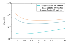
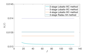
FP bound $\cdot 112$ 2-stage Lobatto IIIC 1.10e-2 4-stage Lobatto IIIC 2.20e-8 3-stage Radau IIA 5.20e-7	FP uniform bound 2-stage Lobatto IIIC 1.35e-2 3-stage Lobatto IIIC 1.40e-2 4-stage Lobatto IIIC 1.35e-2 3-stage Radau IIA 1.36e-2
(a) upper bound $\cdot 112$	(b) uniform bound

Figure 3.1: Numerical bounds for the propagators, and convergence rate versus $J$.

Remark 3.10.

The upper bound in Corollary 3.7 is not optimal. Fig. 3.1(a) shows the numerical upper bounds for the stability functions of two, four-stage Lobatto IIIC method and three-stage Radau IIA method, where the LCPs are more specialized.

Remark 3.11.

In Theorem 3.5, we have derived an upper bound, which however is not sharp. In Fig. 3.1(b), we show the function $k(J)=\sup_{s\in\mathbb{R}_{+}}|\kappa(r,R,J,s)|$, for four methods, i.e., two, three, four-stage Lobatto IIIC and three-stage Radau IIA. Note that we can only define $k(J)$ for the three-stage Lobatto IIIC method for $J\in\mathbb{N}$.

3.4 Parareal efficiency

Maday et al [29] put forth the useful concept of parareal efficiency. Since LCPs have greater complexity than standard ones, e.g. backward Euler scheme, a nuanced evaluation via parareal efficiency is useful. The speed-up, comparing a sequential FP to the parareal algorithm, is defined by

$$\textbf{speed-up}_{\text{para/seq}}(\eta,[0,T])={\textbf{cost}_{\text{seq}}(\eta,[0,T])}/{\textbf{cost}_{\text{para}}(\eta,[0,T])}.$$

In order to achieve a target accuracy $\eta$ for $u^{N_{c}J}$, i.e., $\|u^{N_{c}J}-\overline{u}^{N_{c}J}\|\leq\eta$, with $\overline{u}^{N_{c}J}$ denoting the vaule of the exact propagator at $t=T$, the parareal efficiency is defined as the ratio of the speed-up to the number $N_{c}$ of processors, i.e.,

$$\textbf{eff}_{\text{para/seq}}(\eta,[0,T])=\textbf{speed-up}_{\text{para/seq}}(\eta,[0,T])/{N_{c}}.$$

Throughout, we have ignored the communication cost.

4 Numerical experiments and discussions

Now we present numerical examples to complement the theoretical analysis. We compare LCPs with several commonly employed CPs in terms of optimal convergence factors, and show the parallel efficiency on three model problems. The code for reproducing the numerical experiments will be made available at https://github.com/Qingle-hello/LCPs.git.

4.1 Comparative study on convergence factor

We compare LCP with backward Euler scheme (BE), and the two-stage, second-order singly diagonally implicit Runge Kutta scheme (SDIRK-22) in terms of the mesh-independent convergence factor. The Butcher tableaux and stability function of SDIRK-22 are given respectively by

$\gamma$	$\gamma$	0
1	$(1-\gamma)$	$\gamma$
	$(1-\gamma)$	$\gamma$

and  $R(s)=\dfrac{(2\gamma-1)s+1}{(\gamma s+1)^{2}},$

with $\gamma=\frac{2-\sqrt{2}}{2}$. We take high-order Lobatto IIIC and Radau IIA as the FPs, and learn the LCP using Algorithm 2 with a ratio $J_{0}=16$.

Let $\phi(s)=\kappa(r,R,J,s)$, which varies with the choices of $r$, $R$ and $J$, and take $\phi^{\ast}=\max_{s\in[0,\infty)}\phi(s)$ as the optimal convergence factor (with $s^{\ast}$ being the maximizer). In Table 4.1, we present $\phi^{\ast}$ for different combinations of CPs and FPs: LCPs significantly outperform both BE scheme and SDIRK-22, as indicated by the much smaller convergence factor $\phi^{\ast}$, whereas BE and SDIRK-22 are largely comparable. The improvement is also shown in Figs. 4.1– 4.3, which exhibit pronounced differences in the local maximizer $s^{\ast}$ for BE and SDIRK-22, contrasting sharply with that for LCPs. Furthermore, with the increase of $J$, the variations in $\phi^{\ast}$ and the maximizer $s^{\ast}$ diminish, which agrees with Fig. 3.1.

Table 4.1: The maximum $\phi^{\ast}$ (optimal convergence factor) and maximizer $s^{*}$ of the function $\phi(s)=\kappa(r,R,J,s)$ for three CPs and four FPs.

CP	FP	Stage	Order	Padé approx.
	Lobatto IIIC	2	2	$(0,2)$
	$J$	2	4	16	64	128
BE	$\phi^{\ast}$	0.264	0.287	0.298	0.298	0.298
	$s^{\ast}$	1.65	1.74	1.79	1.79	1.79
SDIRK-22	$\phi^{\ast}$	0.269	0.263	0.262	0.262	0.262
	$s^{\ast}$	7.65	8.01	8.16	8.17	8.17
LCP	$\phi^{\ast}$	0.020	0.014	0.013	0.014	0.014
	$s^{\ast}$	0.73	0.44	10.02	2.37	2.37
	Lobatto IIIC	3	4	$(1,3)$
	$J$	2	4	16	64	128
BE	$\phi^{\ast}$	0.299	0.299	0.298	0.298	0.298
	$s^{\ast}$	1.80	1.79	1.79	1.79	1.79
SDIRK-22	$\phi^{\ast}$	0.261	0.261	0.262	0.262	0.262
	$s^{\ast}$	8.26	8.18	8.17	8.17	8.17
LCP	$\phi^{\ast}$	0.014	0.014	0.014	0.014	0.014
	$s^{\ast}$	2.45	0.39	0.39	0.39	0.39
	Lobatto IIIC	4	6	$(2,4)$
	$J$	2	4	16	64	128
BE	$\phi^{\ast}$	0.298	0.298	0.298	0.298	0.298
	$s^{\ast}$	1.79	1.79	1.79	1.79	1.79
SDIRK-22	$\phi^{\ast}$	0.262	0.262	0.262	0.262	0.262
	$s^{\ast}$	8.17	8.17	8.17	8.17	8.17
LCP	$\phi^{\ast}$	0.014	0.014	0.014	0.014	0.014
	$s^{\ast}$	10.01	10.02	10.02	10.02	10.02
	Radau IIA	3	5	$(2,3)$
	$J$	2	4	16	64	128
BE	$\phi^{\ast}$	0.298	0.298	0.298	0.298	0.298
	$s^{\ast}$	1.79	1.79	1.79	1.79	1.79
SDIRK-22	$\phi^{\ast}$	0.262	0.262	0.262	0.262	0.262
	$s^{\ast}$	8.18	8.17	8.17	8.17	8.17
LCP	$\phi^{\ast}$	0.014	0.014	0.014	0.014	0.014
	$s^{\ast}$	10.26	10.00	10.00	10.00	10.00

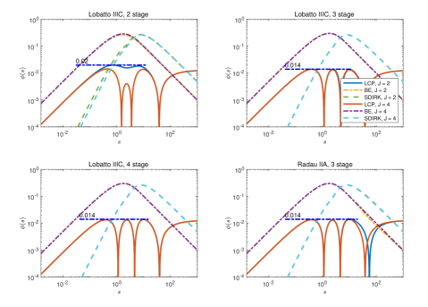
Figure 4.1: The function $\phi(s)$ for three CPs and four FPs when $J\in\{2,4\}$.

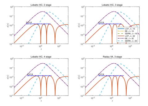
Figure 4.2: The function $\phi(s)$ for three CPs and four FPs when $J\in\{16,32\}$.

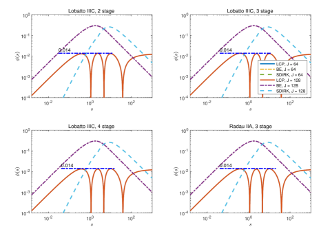
Figure 4.3: The function $\phi(s)$ for three CPs and four FPs when $J\in\{64,128\}$.

4.2 Illustration on model three problems

Next, we show the efficiency of LCPs on one-dimensional linear diffusion models.

Example 4.1.

Consider the following initial-boundary value problem

(20) $$\left\{\begin{aligned} \partial_{t}u(x,t)-\partial_{xx}u(x,t)&=f(x,t),&&x\in\Omega,\,0<t<T,\\ u(x,t)&=0,&&x\in\partial\Omega,\,0<t<T,\\ u(x,0)&=u^{0}(x),&&x\in\Omega.\end{aligned}\right.$$

with $\Omega=(0,\pi)$, and the following three sets of problem data: (a) $T=1$, $u^{0}(x)=x^{10}(x-\pi)^{10}/(\pi/2)^{10}$ and $f\equiv 0$; (b) $T=1$, $u^{0}(x)=\chi_{(0,\pi/2)}(x)$ and $f=\cos(t)\sin(x)$, where $\chi_{(0,\pi/2)}(x)$ denotes the characteristic function of the set $(0,\pi/2)$; (c) $T=100$, $u^{0}(x)=2\chi_{(0,\pi/2)}(x)-1$ and $f=50\sin(2\pi(x+t))$.

In the experiment, we divide the domain $\Omega$ into $M$ equal subintervals, each of length $h=\pi/M$, apply the Galerkin FEM with piesewise linear FEM with a mesh size $h=\pi/1000$, and initialize $U^{n}_{0}$ with the CP. We study the error between the iterative solution $U_{k}^{n}$ by the parareal algorithm and the fine time stepping solution $u^{nJ}$, i.e., $\text{error}=\max_{1\leq n\leq N_{c}}\|U^{n}_{k}-u^{nJ}\|_{L^{2}(\Omega)}$.

The problem data in case (a) is smooth and compatible with the zero Dirichlet boundary condition. In Fig. 4.4, we show the convergence rate of the parareal algorithm with LCPs for two, three, four-stage Lobatto IIIC methods and three-stage Radau IIA method with $J=20$, $100$ and $\Delta t=1/2000$ (i.e., $\Delta T=1/100$ and $1/20$), and take the backward Euler (BE) scheme as the benchmark CP. The convergence property of the parareal algorithm, with backward Euler as the CP, has been studied [41]. LCPs perform much better than BE and is also robust to $J$. The convergence rate of the parareal algorithm with the BE scheme is around 0.3 when $J=100$, as predicted by (5).

The initial data $u_{0}$ in case (b) is nonsmooth. From Fig. 4.4, the convergence rate of the parareal algorithm agrees well with the theoretical predictions from Theorem 3.1 (see also Remark 3.11). Note that for $J=20$, the parareal algorithm with LCPs is two steps faster than that with the BE scheme (for the error tolerance 1.0e-8). The efficiency is accentuated for $J=100$: the learned algorithm is nine steps faster than the standard one.

In Table 4.2, we show the efficiency of the parareal algorithm for case (c), with $J=100$ and a target accuracy $\eta=\text{1.0e-7}$. To achieve the target accuracy, we vary the fine step size with the method, and also exclude the two-stage Lobatto IIIC method due to its low accuracy. The time $t_{n}$ increases with the order of the method increases, but the speed-up decreases due to a shorter time needed to reach the desired accuracy. Meanwhile, the efficiency improves and the cost of ${\mathcal{G}}$ reduces, since maintaining the ratio $J$ requires fewer processors. The comparison between LCPs and BE indicates that despite the increase in its complexity, LCPs better suit the parareal algorithm for linear evolution problems.

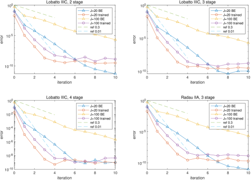
Figure 4.4: The convergence rate for Example 4.1(a) (smooth data).

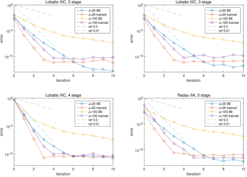
Figure 4.5: The convergence rate for Example 4.1(b) (nonsmooth data).

Table 4.2: The parareal efficiency for Example 4.1(c) (nonsmooth data), with $J=100$ and $\eta=\text{1.0e-7}$.

	three-stage Lobatto		three-stage Radau		four-stage Lobatto
$\Delta t$	1/150		1/45		1/30
Speed-up	BE	LCP	BE	LCP	BE	LCP
w cost ${\mathcal{G}}$	11.48	25.52	4.81	11.03	3.93	10.35
w/o cost ${\mathcal{G}}$	11.51	25.67	4.82	11.05	3.94	10.36
Efficiency	BE	LCP	BE	LCP	BE	LCP
w cost ${\mathcal{G}}$	7.65%	17.02%	10.68%	24.51%	13.09%	34.51%
w/o cost ${\mathcal{G}}$	7.68%	17.11%	10.71%	24.55%	13.10%	34.55%

Next we illustrate the method with a semilinear parabolic problem, the Allen–Cahn equation. It was proposed to describe the motion of anti-phase boundaries in crystalline solids [2], where $u$ denotes the concentration of one of the two metallic components of the alloy and $\epsilon>0$ controls the width of interface.

Example 4.2.

Consider the initial-boundary value problem of the Allen-Cahn equation:

(21) $$\left\{\begin{aligned} \partial_{t}u-\partial_{xx}u&=\epsilon^{-2}(u-u^{3})&&x\in\Omega,\,t\in(0,T],\\ \partial_{x}u(x,t)&=0&&x\in\partial\Omega,\,t\in(0,T],\\ u(x,0)&=u_{0}(x)&&x\in\Omega,\end{aligned}\right.$$

with $\Omega=(0,\pi)$, $T=1$ and $u_{0}=1-2\chi_{(\pi/2,\pi)}$.

In the experiment, we divide the domain $\Omega$ into 1000 equal subintervals of length $h=\pi/1000$ and apply the finite difference method in space. We take the CP $\mathcal{G}$ to be the first-order semi-implicit backward scheme: given $u^{n}$, find $u^{n+1}$ such that

$$u^{n+1}=R(\Delta T{\mathcal{A}})u^{n}+\Delta TP(\Delta T{\mathcal{A}})f({}u^{n}),\quad\text{with }f(u)=\epsilon^{-2}(u-u^{3}).$$

The FP $\mathcal{F}$ is a fully implicit, high-order, single step integrator, e.g., Lobatto IIIC or fully implicit Radau schemes: given $u^{n}$, we find $u^{n+1}$ such that

(22) $$\begin{cases}u^{ni}=u^{n-1}+\Delta t\sum^{m}_{j=1}a_{ij}({\mathcal{A}}u^{nj}+f(u^{nj})),&\\ u^{n}=u^{n-1}+\Delta t\sum^{m}_{i=1}b_{i}({\mathcal{A}}u^{ni}+f(u^{ni})).&\end{cases}$$

Here, $u^{ni}$ denotes the interstage of the implicit single step integrator. If the time step size $\Delta t$ is small, the nonlinear system (22) is uniquely solvable, e.g., via Newton’s algorithm. Since the FP $\mathcal{F}$ is fully nonlinear, it is time consuming to numerically realize the scheme, whereas the CP $\mathcal{G}$ is a linear scheme, so the parareal algorithm may greatly improve the efficiency.

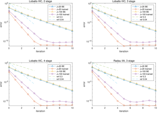
Figure 4.6: The convergence rate for Example 4.2 (Allen–Cahn equation) with $\epsilon^{2}=1$.

In the experiment, we take $\epsilon^{2}\in\{1,0.02\}$. In Fig. 4.6, for $\epsilon^{2}=1$, we illustrate LCPs with $J=20$, $100$ and $\Delta t=1/2000$ (i.e., $\Delta T=1/100$ and $1/20$). The results show that the convergence rate of the parareal algorithm, using LCPs, is approximately $0.04$, compared to $0.3$ with the BE scheme. Moreover, an increase in $J$ corresponds to a larger $\Delta T$, limiting the CP’s capability to accurately capture the solution structure. Thus, the convergence rate deteriorates as $J$ increases. In Fig. 4.7, for $\epsilon^{2}=0.02$, we illustrate LCPs with $J=10,$ $20$ and $\Delta t=1/10000$ (i.e., $\Delta T=1/1000$ and $1/500$). For $J=10$, $20$, the convergence rate of LCPs is about $0.04$. However, for larger $J$, the difference between the BE scheme and LCPs is small, calling for modifications of LCPs for nonlinear problems, especially for small $\epsilon$. In Table 4.3, we show the parareal efficiency for $\epsilon^{2}=1$, $T=10$, $J=20$ and a target accuracy $\eta=\text{1.0e-6}$. The trend of speed-up and efficiency is consistent with Table 4.2. However, the strong nonlinearity renders the efficiency improvement less pronounced.

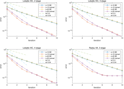
Figure 4.7: The convergence rate for Example 4.2 (Allen–Cahn equation) with $\epsilon^{2}=0.02$.

Table 4.3: The parareal efficiency for Example 4.2 with $\epsilon^{2}=1$, $T=10$, $J=20$ and $\eta=\text{1.0e-6}$.

	three-stage Lobatto		three-stage Radau		four-stage Lobatto
$\Delta t$	1/300		1/100		1/80
Speed-up	BE	LCP	BE	LCP	BE	LCP
w cost ${\mathcal{G}}$	10.93	18.78	3.65	7.90	3.43	11.63
w/o cost ${\mathcal{G}}$	11.62	19.70	3.74	8.40	3.48	11.90
Efficiency	BE	LCP	BE	LCP	BE	LCP
w cost ${\mathcal{G}}$	7.29%	12.52%	7.27%	15.80%	8.59%	29.08%
w/o cost ${\mathcal{G}}$	7.75%	13.13%	7.48%	16.80%	8.69%	29.75%

The third and last example is about viscous Burgers’ equation, which is a model problem in fluid dynamics, describing e.g., the decay of turbulence within a box.

Example 4.3.

Fix $T=1$, and $u_{0}(x)=\chi_{(0,1/2)}(x).$ Consider the viscous Burgers’ equation

$$\left\{\begin{aligned} \partial_{t}u+u\partial_{x}u&=\nu\partial_{xx}u,&&x\in(0,1),\,t\in(0,T],\\ u(0,t)&=u(1,t)=0,&&t\in(0,T],\\ u(x,0)&=u_{0}(x),&&x\in(0,1).\end{aligned}\right.$$

We take $\nu\in\{1,0.02\}$ in the experiment. In Fig. 4.8, for $\nu=1$, we examine LCPs with $J=20$, $100$ and $\Delta t=1/2000$ (i.e., $\Delta T=1/100$ and $1/20$). The results show that the convergence rate of the parareal algorithm, with LCPs, is approximately $0.04$, which agree well with that in Fig. 4.6. In Fig. 4.7, for the more challenging case $\nu=0.02$, we evaluate LCPs with $J=10,100$ and $\Delta t=1/10000$ (i.e., $\Delta T=1/1000$ and $1/100$). For $J=10$, the convergence rate of LCPs is approximately 0.06, whereas that for BE is around 0.21. Remarkably, the ratio $\Delta T/\nu$ is unchanged for $J=100$ in the linear case, cf. Fig. 4.8, so their behaviors are similar. This phenomenon has been analyzed for linear advection-diffusion cases in [15]. For $J=100$, both the parareal algorithm and the standard one exhibit slower convergence. Nonetheless, LCP is still competitive with the BE CP.

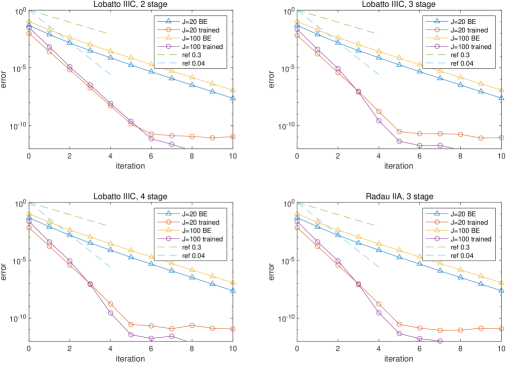
Figure 4.8: The convergence rate for Example 4.3 (viscous Burgers’ equation) with $\nu=1$.

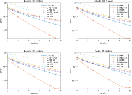
Figure 4.9: The convergence rate for Example 4.3 (viscous Burgers’ equation) with $\nu=0.02$.

5 Conclusion

We have explored the potential of learning coarse propagators in parareal algorithms to overcome the barrier in convergence order. The approach is based on rigorous error estimation for linear evolution problems, which ensures that the LCPs enjoy highly desirable properties, e.g., stability and consistent order. We have developed a systematic procedure for the learning of the CP. The numerical experiments fully confirm the theoretical prediction, including mildly nonlinear problems. Most remarkably, even for highly nonlinear problems, the LCPs can still outperform the classical BE scheme. One important question is to extend the idea to far more challenging situations, e.g., highly nonlinear problems, multiscale problems [26], and hyperbolic problems [10]. Also it is promising to develop the learning strategy for other parallel-in-time algorithms, e.g., the two-level MGRIT algorithm with FCF-smoother [35, 13].

Appendix A Explicit formulas of LCPs

In this appendix, we present the explicit formulas of LCPs, for $q=1$, $C_{1}^{0}=1$ and $J_{0}=16$. (1) For two-stage Lobatto IIIC method,

$$R_{2}(\lambda) =\frac{{1.0-0.20967\lambda+0.00484\lambda^{2}}}{{1.0+0.79033\lambda+0.37931\lambda^{2}}}\quad\mbox{and}\quad P_{1}(\lambda)=\frac{1.0+0.37447\lambda}{1.0+0.79033\lambda+0.37931\lambda^{2}}.$$

(2) For three-stage Lobatto IIIC method,

$$R_{3}(\lambda) =\frac{{1.0-0.21014\lambda+0.00486\lambda^{2}}}{{1.0+0.78986\lambda+0.38283\lambda^{2}}}\quad\mbox{and}\quad P_{1}(\lambda)=\frac{1.0+0.37797\lambda}{1.0+0.78986\lambda+0.38283\lambda^{2}}.$$

(3) For four-stage Lobatto IIIC method,

$$R_{4}(\lambda) =\frac{{1.0-0.21091\lambda+0.00476\lambda^{2}}}{{1.0+0.78909\lambda+0.37898\lambda^{2}}}\quad\mbox{and}\quad P_{1}(\lambda)=\frac{1.0+0.37422\lambda}{1.0+0.78909\lambda+0.37898\lambda^{2}}.$$

(4) For three-stage Radau IIA method,

$$R_{r}(\lambda) =\frac{{1.0-0.21125\lambda+0.00479\lambda^{2}}}{{1.0+0.78875\lambda+0.37922\lambda^{2}}}\quad\mbox{and}\quad P_{1}(\lambda)=\frac{1.0+0.37443\lambda}{1.0+0.78875\lambda+0.37922\lambda^{2}}.$$

In Fig. A.1, we show the stability functions of LCPs and the corresponding fine propagators. It is observed that they are all stable approximations of $e^{-\lambda}$ around $\lambda=0$.

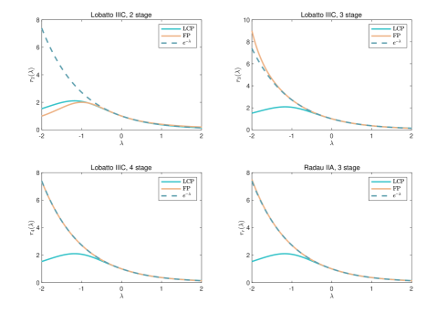
Figure A.1: The stability functions of the LCPs, for four FPs.

References

- [1] W. Agboh, O. Grainger, D. Ruprecht, and M. Dogar, Parareal with a learned coarse model for robotic manipulation, Comput. Vis. Sci., 23 (2020), pp. Paper No. 8, 10.
- [2] J. W. Allen, S. M.; Cahn, Ground state structures in ordered binary alloys with second neighbor interactions, Acta Metall., 20 (1972), pp. 423–433.
- [3] G. Ariel, S. J. Kim, and R. Tsai, Parareal multiscale methods for highly oscillatory dynamical systems, SIAM J. Sci. Comput., 38 (2016), pp. A3540–A3564.
- [4] G. Bal, On the convergence and the stability of the parareal algorithm to solve partial differential equations, in Domain decomposition methods in science and engineering, vol. 40 of Lect. Notes Comput. Sci. Eng., Springer, Berlin, 2005, pp. 425–432.
- [5] G. Bal and Y. Maday, A “parareal” time discretization for non-linear PDE’s with application to the pricing of an American put, in Recent developments in domain decomposition methods (Zürich, 2001), vol. 23 of Lect. Notes Comput. Sci. Eng., Springer, Berlin, 2002, pp. 189–202.
- [6] Y. Bar-Sinai, S. Hoyer, J. Hickey, and M. P. Brenner, Learning data-driven discretizations for partial differential equations, Proc. Natl. Acad. Sci. USA, 116 (2019), pp. 15344–15349.
- [7] P. Bianchi, W. Hachem, and S. Schechtman, Convergence of constant step stochastic gradient descent for non-smooth non-convex functions, Set-Valued Var. Anal., 30 (2022), pp. 1117–1147.
- [8] C.-E. Brehier and X. Wang, On parareal algorithms for semilinear parabolic stochastic PDEs, SIAM J. Numer. Anal., 58 (2020), pp. 254–278.
- [9] P. Brenner, M. Crouzeix, and V. Thomée, Single-step methods for inhomogeneous linear differential equations in Banach space, RAIRO Anal. Numér., 16 (1982), pp. 5–26.
- [10] H. De Sterck, R. D. Falgout, S. Friedhoff, O. A. Krzysik, and S. P. MacLachlan, Optimizing multigrid reduction-in-time and parareal coarse-grid operators for linear advection, Numer. Linear Algebra Appl., 28 (2021), pp. Paper No. e2367, 22.
- [11] B. L. Ehle, On Padé approximations to the exponential function and A-stable methods for the numerical solution of initial value problems, PhD thesis, University of Waterloo, Waterloo, Ontario, 1969.
- [12] S. Engblom, Parallel in time simulation of multiscale stochastic chemical kinetics, Multiscale Model. Simul., 8 (2009), pp. 46–68.
- [13] S. Friedhoff and B. S. Southworth, On “optimal” -independent convergence of parareal and multigrid-reduction-in-time using Runge-Kutta time integration, Numer. Linear Algebra Appl., 28 (2021), pp. Paper No. e2301, 30.
- [14] M. J. Gander, 50 years of time parallel time integration, in Multiple shooting and time domain decomposition methods, vol. 9 of Contrib. Math. Comput. Sci., Springer, Cham, 2015, pp. 69–113.
- [15] M. J. Gander and T. Lunet, A Reynolds number dependent convergence estimate for the parareal algorithm, in Domain decomposition methods in science and engineering XXV, vol. 138 of Lect. Notes Comput. Sci. Eng., Springer, Cham, 2020, pp. 277–284.
- [16] M. J. Gander and S. Vandewalle, Analysis of the parareal time-parallel time-integration method, SIAM J. Sci. Comput., 29 (2007), pp. 556–578.
- [17] J.-L. Goffin, On convergence rates of subgradient optimization methods, Mathematical programming, 13 (1977), pp. 329–347.
- [18] G. H. Golub and C. F. Van Loan, Matrix computations, Johns Hopkins University Press, Baltimore, MD, fourth ed., 2013.
- [19] D. Greenfeld, M. Galun, R. Basri, I. Yavneh, and R. Kimmel, Learning to optimize multigrid PDE solvers, in Proceedings of the International Conference on Machine Learning, 2019, pp. 2415–2423.
- [20] Y. Guo, F. Dietrich, T. Bertalan, D. T. Doncevic, M. Dahmen, I. G. Kevrekidis, and Q. Li, Personalized algorithm generation: a case study in learning ODE integrators, SIAM J. Sci. Comput., 44 (2022), pp. A1911–A1933.
- [21] E. Hairer and G. Wanner, Solving ordinary differential equations. II, Springer-Verlag, Berlin, second ed., 1996.
- [22] E. Hairer and G. Wanner, Stiff differential equations solved by Radau methods, J. Comput. Appl. Math., 111 (1999), pp. 93–111.
- [23] R. Huang, R. Li, and Y. Xi, Learning optimal multigrid smoothers via neural networks, SIAM J. Sci. Comput., 45 (2023), pp. S199–S225.
- [24] A. Q. Ibrahim, S. Götschel, and D. Ruprecht, Parareal with a physics-informed neural network as coarse propagator. Preprint, arXiv:2303.03848, 2023.
- [25] A. Khaled and P. Richtárik, Better theory for SGD in the nonconvex world, Trans. Machine Learn. Res., (2023).
- [26] G. Li and J. Hu, Wavelet-based edge multiscale parareal algorithm for parabolic equations with heterogeneous coefficients and rough initial data, J. Comput. Phys., 444 (2021), pp. 10572, 18.
- [27] J.-L. Lions, Y. Maday, and G. Turinici, Résolution d’EDP par un schéma en temps “pararéel”, C. R. Acad. Sci. Paris Sér. I Math., 332 (2001), pp. 661–668.
- [28] D. G. Luenberger and Y. Ye, Linear and nonlinear programming, Springer, New York, third ed., 2008.
- [29] Y. Maday and O. Mula, An adaptive parareal algorithm, J. Comput. Appl. Math., 377 (2020), pp. 112915, 18.
- [30] T. P. Mathew, M. Sarkis, and C. E. Schaerer, Analysis of block parareal preconditioners for parabolic optimal control problems, SIAM J. Sci. Comput., 32 (2010), pp. 1180–1200.
- [31] S. Mishra, A machine learning framework for data driven acceleration of computations of differential equations, Math. Eng., 1 (2019), pp. 118–146.
- [32] H. Nguyen and R. Tsai, Numerical wave propagation aided by deep learning, J. Comput. Phys., 475 (2023), pp. Paper No. 111828, 26.
- [33] G. Pagès, O. Pironneau, and G. Sall, The parareal algorithm for American options, C. R. Math. Acad. Sci. Paris, 354 (2016), pp. 1132–1138.
- [34] K. Scaman, C. Malherbe, and L. Dos Santos, Convergence rates of non-convex stochastic gradient descent under a generic Lojasiewicz condition and local smoothness, in International Conference on Machine Learning, PMLR, 2022, pp. 19310–19327.
- [35] B. S. Southworth, Necessary conditions and tight two-level convergence bounds for parareal and multigrid reduction in time, SIAM J. Matrix Anal. Appl., 40 (2019), pp. 564–608.
- [36] V. Thomée, Galerkin finite element methods for parabolic problems, Springer-Verlag, Berlin, second ed., 2006.
- [37] S.-L. Wu, Convergence analysis of some second-order parareal algorithms, IMA J. Numer. Anal., 35 (2015), pp. 1315–1341.
- [38] S.-L. Wu and T. Zhou, Convergence analysis for three parareal solvers, SIAM J. Sci. Comput., 37 (2015), pp. A970–A992.
- [39] Q. Xu, J. S. Hesthaven, and F. Chen, A parareal method for time-fractional differential equations, J. Comput. Phys., 293 (2015), pp. 173–183.
- [40] G. R. Yalla and B. Engquist, Parallel in time algorithms for multiscale dynamical systems using interpolation and neural networks, in HPC ’18: Proceedings of the High Performance Computing Symposium, 2018, pp. 9, 1–12.
- [41] J. Yang, Z. Yuan, and Z. Zhou, Robust convergence of parareal algorithms with arbitrarily high-order fine propagators, CSIAM Trans. Appl. Math., 4 (2023), pp. 566–591.
- [42] K. Yosida, Functional analysis, Springer-Verlag, Berlin, 1995.