Singular layer Physics Informed Neural Network method for Plane Parallel Flows

Abstract.

We construct in this article the semi-analytic Physics Informed Neural Networks (PINNs), called singular layer PINNs (or sl-PINNs), that are suitable to predict the stiff solutions of plane-parallel flows at a small viscosity. Recalling the boundary layer analysis, we first find the corrector for the problem which describes the singular behavior of the viscous flow inside boundary layers. Then, using the components of the corrector and its curl, we build our new sl-PINN predictions for the velocity and the vorticity by either embedding the explicit expression of the corrector (or its curl) in the structure of PINNs or by training the implicit parts of the corrector (or its curl) together with the PINN predictions. Numerical experiments confirm that our new sl-PINNs produce stable and accurate predicted solutions for the plane-parallel flows at a small viscosity.

1. Introduction

We aim in this article to construct a version of Physics Informed Neural Networks (PINNs) to predict the motion of certain symmetric flows especially when the viscosity is very small. To this end, we consider the stationary Navier-Stokes equations (NSE) in a periodic channel domain $\Omega:=(0,L)^{2}_{\text{per}}\times(0,1)$ when a symmetry imposed to the velocity vector field $\boldsymbol{u}^{\varepsilon}$ (sol. to NSE at a small viscosity $\varepsilon>0$) is given in the form,

$$\boldsymbol{u}^{\varepsilon}=(u^{\varepsilon}_{1}(z),\,u^{\varepsilon}_{2}(x,z),\,0).$$ (1.1)

Then the stationary NSE are reduced to:

$$\left\{\begin{array}[]{rl}\vspace{1.5mm}u^{\varepsilon}_{1}-\varepsilon{d^{2}_{z}u^{\varepsilon}_{1}}&=f_{1},\quad\text{in }\Omega,\\ \vspace{1.5mm}u^{\varepsilon}_{2}-\varepsilon{\partial^{2}_{x}u^{\varepsilon}_{2}}-\varepsilon{\partial^{2}_{z}u^{\varepsilon}_{2}}+u^{\varepsilon}_{1}\,{\partial_{x}u^{\varepsilon}_{2}}&=f_{2},\quad\text{in }\Omega,\\ \vspace{1.5mm}u^{\varepsilon}_{2}\text{ is periodic}&\text{in $x$ with period $L$},\\ u^{\varepsilon}_{i}&=0,\quad i=1,2,\text{ on }\Gamma,\text{ i.e., at }z=0,1,\end{array}\right.$$ (1.2)

provided that the smooth data $\boldsymbol{f}$, which is periodic in $x$, satisfies the symmetry in (1.1) as well. The fluid motion, associated with our model equations (1.2), occurs in the tangential directions in $x$ and $y$, i.e., $u^{\varepsilon}_{1}$ and $u^{\varepsilon}_{2}$, depending on the tangential variable $x$ and the normal variable $z$ in $\Omega$. Here and throughout this article, we use the notations, $d_{z}=d/dz$, $\partial_{x}=\partial/\partial_{x}$, and $\partial_{z}=\partial/\partial_{z}$.

We now introduce the vorticity of the Navier-Stokes solutions,

$$\boldsymbol{\omega}^{\varepsilon}=(\omega^{\varepsilon}_{1}(x,z),\omega^{\varepsilon}_{2}(z),\omega^{\varepsilon}_{3}(x,z)):=\textnormal{curl }\boldsymbol{u}^{\varepsilon}=\big{(}-\partial_{z}u^{\varepsilon}_{2},\,d_{z}u^{\varepsilon}_{1},\,\partial_{x}u^{\varepsilon}_{2}\big{)}.$$ (1.3)

By computing $-\partial_{z}$(1.2)₂, $d_{z}$(1.2)₁, and $\partial_{x}$(1.2)₂, we write the vorticity formulation of NSE (1.2) in the form,

$$\left\{\begin{array}[]{rl}\vspace{1.5mm}\omega^{\varepsilon}_{1}-\varepsilon{\partial^{2}_{x}\omega^{\varepsilon}_{1}}-\varepsilon{\partial^{2}_{z}\omega^{\varepsilon}_{1}}-\omega^{\varepsilon}_{2}\,\omega^{\varepsilon}_{3}+u^{\varepsilon}_{1}\,{\partial_{x}\omega^{\varepsilon}_{1}}&=-\partial_{z}f_{2},\quad\text{in }\Omega,\\ \vspace{1.5mm}\omega^{\varepsilon}_{2}-\varepsilon{d^{2}_{z}\omega^{\varepsilon}_{2}}&=d_{z}f_{1},\quad\text{in }\Omega,\\ \vspace{1.5mm}\omega^{\varepsilon}_{3}-\varepsilon{\partial^{2}_{x}\omega^{\varepsilon}_{3}}-\varepsilon{\partial^{2}_{z}\omega^{\varepsilon}_{3}}+u^{\varepsilon}_{1}\,{\partial_{x}\omega^{\varepsilon}_{3}}&=\partial_{x}f_{2},\quad\text{in }\Omega,\\ \omega^{\varepsilon}_{i}\text{ is periodic}&\text{in $x$ with period $L$, $i=1,3$}.\end{array}\right.$$ (1.4)

To derive a set of proper boundary conditions for the vorticity, we apply the Lighthill principle by restricting (1.2)_1,2 on $\Gamma$, and using (1.2)₄; see, e.g., [14] as well. Then we obtain the boundary conditions for $\boldsymbol{\omega}^{\varepsilon}$ as

$$\left\{\begin{array}[]{rl}\vspace{1.5mm}\partial_{z}\omega^{\varepsilon}_{1}&=\dfrac{1}{\varepsilon}f_{2},\quad\text{on }\Gamma,\\ \vspace{1.5mm}d_{z}\omega^{\varepsilon}_{2}&=-\dfrac{1}{\varepsilon}f_{1},\quad\text{on }\Gamma,\\ \vspace{1.5mm}\omega^{\varepsilon}_{3}&=0,\quad\text{on }\Gamma.\end{array}\right.$$ (1.5)

Setting $\varepsilon=0$ in the NSE (1.2) and (1.4), we find that the inviscid limits $\boldsymbol{u}^{0}=(u^{0}_{1}(z),\,u^{0}_{2}(x,z),\,0)$ of $\boldsymbol{u}^{\varepsilon}$ and $\boldsymbol{\omega}^{0}=\text{curl }\boldsymbol{u}^{0}$ of $\boldsymbol{\omega}^{\varepsilon}$ satisfy the following equations:

$$\left\{\begin{array}[]{rl}\vspace{1.5mm}u^{0}_{1}&=f_{1},\quad\text{in }\Omega,\\ \vspace{1.5mm}u^{0}_{2}+u^{0}_{1}\,{\partial_{x}u^{0}_{2}}&=f_{2},\quad\text{in }\Omega,\\ u^{0}_{2}\text{ is periodic}&\text{in $x$ with period $L$}.\end{array}\right.$$ (1.6)

$$\left\{\begin{array}[]{rl}\vspace{1.5mm}\omega^{0}_{1}-\omega^{0}_{2}\,\omega^{0}_{3}+u^{0}_{1}\,{\partial_{x}\omega^{0}_{1}}&=-\partial_{z}f_{2},\quad\text{in }\Omega,\\ \vspace{1.5mm}\omega^{0}_{2}&=d_{z}f_{1},\quad\text{in }\Omega,\\ \vspace{1.5mm}\omega^{0}_{3}+u^{0}_{1}\,{\partial_{x}\omega^{0}_{3}}&=\partial_{x}f_{2},\quad\text{in }\Omega,\\ \omega^{0}_{i}\text{ is periodic}&\text{in $x$ with period $L$, $i=1,3$}.\end{array}\right.$$ (1.7)

Under a sufficient regularity assumption on the data $f$, the well-posedness of (1.2), (1.4), (1.6) or (1.7), and the asymptotic behavior of solutions to (1.2) and (1.4) are fully investigated in [10] and [14] (for the time dependent case). More precisely, following the methodology of boundary layer analysis from, e.g., [13, 18, 32], it is verified in those earlier works that, as the viscosity $\varepsilon$ vanishes, the Navier-Stokes solution $\boldsymbol{u}^{\varepsilon}$ converges strongly in $L^{2}$ to the Euler solution $\boldsymbol{u}^{0}$ and that the corresponding Navier-Stokes vorticity $\boldsymbol{\omega}^{\varepsilon}$ converges to the Euler vorticity $\boldsymbol{\omega}^{0}$ in a certain weak sense, up to a positive measure supported on the boundary. Here we briefly recall this result from [10]:

Theorem 1.1.

Under a sufficient regularity assumption on the data $\boldsymbol{f}$, e.g., $\boldsymbol{f}\in H^{6}(\Omega)$, the viscous plane-parallel solution $\boldsymbol{u}^{\varepsilon}$ converges to the corresponding inviscid solution $\boldsymbol{u}^{0}$ in the sense that

$$\|\boldsymbol{u}^{\varepsilon}-\boldsymbol{u}^{0}\|_{L^{2}(\Omega)}\leq\kappa\varepsilon^{\frac{1}{4}},\quad\text{ as }\varepsilon\rightarrow 0.$$ (1.8)

In addition, as $\varepsilon\rightarrow 0$, we have

$$\lim_{\varepsilon\rightarrow 0}\big{(}\boldsymbol{\omega}^{\varepsilon},\,\boldsymbol{\psi}\big{)}_{L^{2}(\Omega)}=\big{(}\boldsymbol{\omega}^{0},\,\boldsymbol{\psi}\big{)}_{L^{2}(\Omega)}+\big{(}\boldsymbol{u}^{0}|_{\Gamma}\times\boldsymbol{n},\,\boldsymbol{\psi}\big{)}_{L^{2}(\Gamma)},\quad\forall\boldsymbol{\psi}\in C(\overline{\Omega}),$$ (1.9)

which expresses the fact that

$$\lim_{\varepsilon\rightarrow 0}\boldsymbol{\omega}^{\varepsilon}=\boldsymbol{\omega}^{0}+(\boldsymbol{u}^{0}|_{\Gamma}\times\boldsymbol{n})\delta_{\Gamma},$$ (1.10)

in the sense of weak^∗ convergence of bounded measures on $\overline{\Omega}$.

In proving Theorem 1.1 in [10] and [14], the authors employed the method of matching asymptotic expansions and introduce an expansion of $\boldsymbol{u}^{\varepsilon}$ (hence of $\boldsymbol{\omega}^{\varepsilon}$) at a small $\varepsilon$ in the form,

$$\boldsymbol{u}^{\varepsilon}\simeq\boldsymbol{u}^{0}+\boldsymbol{\varphi},\qquad\boldsymbol{\omega}^{\varepsilon}\simeq\boldsymbol{\omega}^{0}+\text{curl }\boldsymbol{\varphi},$$

by constructing an artificial function $\boldsymbol{\varphi}$, called corrector, which describes the singular behavior of $\boldsymbol{u}^{\varepsilon}-\boldsymbol{u}^{0}$ near the boundary $\Gamma$; see below Section 2 for more information about the asymptotic expansion above and the corrector $\boldsymbol{\varphi}$. In fact, performing involved analysis, the authors verify the validity at a small viscosity of the asymptotic expansion in the sense that

$$\left\{\begin{array}[]{l}\vspace{1.5mm}\|\overline{{u}}_{1}\|_{L^{2}(\Omega)}+\varepsilon^{\frac{1}{2}}\|d_{z}\overline{{u}}_{1}\|_{L^{2}(\Omega)}\leq\kappa\varepsilon,\\ \vspace{1.5mm}\|\overline{{u}}_{2}\|_{L^{2}(\Omega)}+\varepsilon^{\frac{1}{2}}\|\nabla\overline{{u}}_{2}\|_{L^{2}(\Omega)}\leq\kappa\varepsilon,\\ \vspace{1.5mm}{\|\overline{\omega}_{1}\|_{L^{2}(\Omega)}+\varepsilon^{\frac{1}{2}}\|\nabla\overline{\omega}_{1}\|_{L^{2}(\Omega)}\leq\kappa\varepsilon^{\frac{1}{2}},}\\ \vspace{1.5mm}\|\overline{\omega}_{2}\|_{L^{2}(\Omega)}+\varepsilon^{\frac{1}{2}}\|d_{z}\overline{\omega}_{2}\|_{L^{2}(\Omega)}\leq\kappa\varepsilon^{\frac{3}{4}},\\ {\|\overline{\omega}_{3}\|_{L^{2}(\Omega)}+\varepsilon^{\frac{1}{2}}\|\nabla\overline{\omega}_{3}\|_{L^{2}(\Omega)}\leq\kappa\varepsilon,}\end{array}\right.$$ (1.11)

where the difference between the viscous solution $\boldsymbol{u}^{\varepsilon}$ and the proposed expansion $\boldsymbol{u}^{0}+\boldsymbol{\varphi}$ is defined by

$$\overline{\boldsymbol{u}}=\boldsymbol{u}^{\varepsilon}-(\boldsymbol{u}^{0}+\boldsymbol{\varphi}),\qquad\overline{\boldsymbol{\omega}}=\text{curl }\overline{\boldsymbol{u}}.$$

Then, thanks to the properties of the corrector, Theorem 1.1 follows from (1.11).

It is well-understood that a singular perturbation problem, such as our model (1.2) or (1.4) - (1.5), generates a thin layer near the boundary, called boundary layer, where a sharp transition of the solution occurs; see, e.g., [13, 18, 28, 32]. Generally speaking, when we approximate a solution to any singularly perturbed boundary value problem, a very large computational error is created near the boundary, because of the stiffness nature of the solution inside boundary layers. Hence, to achieve a sufficiently accurate approximate solution, especially near the boundary, certain additional treatments are proposed and successfully employed, e.g., mesh refinements inside boundary layers [30, 34] and semi-analytic methods using the boundary layer corrector [10, 12, 16, 19]. The main idea of the semi-analytic method or the mesh refinement method is to provide more information about the solution or introduce more finer approximation of the solution inside the boundary layer. These enriched methods have proven to be highly efficient to approximate the solutions of singularly perturbed boundary value problems.

Neural networks, in particular the Physics Informed Neural Networks (PINNs), have developed as an important and effective tool for predicting solutions to partial differential equations. One special feature of PINNs is that the loss function is defined based on a residual from the differential equation under consideration where the collocation points in the time-space domain are used as the input for the neural network. This property makes PINNs well-suited particularly for solving time-dependent, multi-dimensional equations in a domain involved in complex geometries, see, e.g., [22, 25, 24, 29, 31, 37, 23, 27, 21, 26, 33, 36, 35]. Although the PINNs have become a popular tool in scientific machine learning, there is an well-known issue on their robustness for certain types of problems, including singularly perturbed boundary value problems. As investigated in some recent works, e.g., [1, 3, 5, 6, 4, 2, 15, 17, 20, 25], the PINNs experience some limitations to capture a singular behavior of solutions, e.g., inside a boundary/interior layer. Hence it is of great interest to overcome this challenging task by developing a methodology to build a version of robust and reliable PINN methods for singular perturbations.

In a series of recent papers [7, 8, 9], the authors suggested a new semi-analytic approach to enrich the conventional PINN methods applied to boundary layer problems. In fact, using the so-called corrector (which describes the singular behavior of the solution inside boundary/interior layers), the authors construct a version of PINNs enriched by the corrector and this new semi-analytic PINNs are proven to outperform the conventional PINNs for the 1 or 2D singularly perturbed elliptic/parabolic equations tested in the papers.

Following the methodology in [7, 8, 9], we aim in this article to construct the semi-analytic PINNs, called singular layer PINNs (or sl-PINNs), that are suitable to predict the stiff solutions of plane-parallel flows at a small viscosity. To this end, in Section 2 below, we first recall from [14, 13, 10] the asymptotic expansions for (1.2) and (1.4) - (1.5). Then, using the corresponding boundary layer analysis, we construct our new singular layer PINNs (sl-PINNs) for the velocity vector field in Sections 3.1 - 3.2, and (sl-PINNs) for the vorticity in Section 4.1. The numerical computations for our sl-PINNs with a comparison with those from the conventional PINNs appear in Section 3.3 for the velocity and 4.2 for the vorticity. It is verified numerically that our novel sl-PINNs capture well the sharp transition and hence produce good predicted solutions for the stiff plane-parallel flows.

2. Boundary layer analysis

We recall briefly from [10] the boundary layer analysis for our model systems (1.2) and (1.5):

We propose an asymptotic expansion of $\boldsymbol{u}^{\varepsilon}$, solution of (1.2), as

$$\boldsymbol{u}^{\varepsilon}\simeq\boldsymbol{u}^{0}+\boldsymbol{\varphi},$$ (2.1)

where $\boldsymbol{\varphi}$ is the corrector, which will be constructed below, in the form,

$$\boldsymbol{\varphi}=\big{(}\varphi_{1}(z),\,\varphi_{2}(x,z),\,0\big{)}.$$ (2.2)

Inserting $\boldsymbol{\varphi}$ into the difference between the equations (1.2) and (1.6), we collect all the terms of dominant order $\varepsilon^{0}$ and write the asymptotic equation for $\boldsymbol{\varphi}$ as the weakly coupled system below:

$$\left\{\begin{array}[]{rl}\vspace{1.5mm}\displaystyle\varphi_{1}-\varepsilon{d^{2}_{z}\varphi_{1}}&=0,\quad\text{in }\Omega,\\ \vspace{1.5mm}\displaystyle\varphi_{2}-\varepsilon\Delta\varphi_{2}+\big{(}\varphi_{1}+u^{0}_{1}\big{)}{\partial_{x}\varphi_{2}}+\varphi_{1}{\partial_{x}u^{0}_{2}}&=0,\quad\text{in }\Omega,\\ \varphi_{i}&=-u^{0}_{i},\quad\text{on }\Gamma,\text{ }i=1,2.\end{array}\right.$$ (2.3)

To construct the corrector $\boldsymbol{\varphi}$ as an (approximate) solution of (2.3) above, we introduce a $C^{\infty}$ truncation function $\sigma_{L}$ (and $\sigma_{R}$) near the boundary at $z=0$ (and $z=1$) such that

$$\begin{array}[]{ccc}\sigma_{L}(z)=\left\{\begin{array}[]{l}\vspace{1.5mm}1,\text{ }0\leq z\leq 1/4,\\ 0,\text{ }z\geq 1/2,\end{array}\right.&&\sigma_{R}(z)=\sigma_{L}(1-z).\end{array}$$ (2.4)

Using the truncations in (2.4), we define the first component $\varphi_{1}$ of the corrector as

$$\varphi_{1}(z)=\sigma_{L}(z)\,\varphi_{1,\,L}(z)+\sigma_{R}(z)\,\varphi_{1,\,R}(z),$$ (2.5)

where

$$\varphi_{1,\,L}(z)=-u^{0}_{1}(0)\,e^{-z/\sqrt{\varepsilon}},\qquad\qquad\varphi_{1,\,R}(z)=-u^{0}_{1}(1)\,e^{-(1-z)/\sqrt{\varepsilon}}.$$ (2.6)

One can verify that ${\varphi}_{1}$ enjoys the estimates,

$$\|{d_{z}^{m}\varphi_{1}}\|_{L^{p}(\Omega)}\leq\kappa\varepsilon^{\frac{1}{2p}-\frac{m}{2}},\quad m\geq 0,\quad 1\leq p\leq\infty,$$ (2.7)

as well as the proposed asymptotic equation in (2.3),

$$\left\{\begin{array}[]{rl}\vspace{1.5mm}\displaystyle{\varphi_{1}}-\varepsilon{d^{2}_{z}\varphi_{1}}&=e.s.t.,\quad\text{in }\Omega,\\ \displaystyle\varphi_{1}&=-u^{0}_{1},\quad\text{on }\Gamma,\end{array}\right.$$ (2.8)

where $e.s.t.$ denotes a term that is exponentially small with respect to the small viscosity parameter $\varepsilon$ in the spaces, e.g., $C^{s}(\Omega)$ or $H^{s}(\Omega)$, $0\leq s\leq\infty$.

Using the first component $\varphi_{1}$, we define $\varphi_{2,\,L}$ and $\varphi_{2,\,R}$ as the solutions of

$$\left\{\begin{array}[]{rl}\vspace{1.5mm}\displaystyle{\varphi_{2,\,L}}-\varepsilon\Delta\varphi_{2,\,L}+\big{(}\varphi_{1,\,L}+u^{0}_{1}\big{)}{\partial_{x}\varphi_{2,\,L}}&=-\varphi_{1,\,L}\,{\partial_{x}u^{0}_{2}},\quad z>0,\\ \vspace{1.5mm}\varphi_{2,\,L}\text{ is}&\text{$L$-periodic in }x,\\ \vspace{1.5mm}\displaystyle\varphi_{2,\,L}&=-u^{0}_{2},\quad z=0,\\ \varphi_{2,\,L}&\rightarrow 0,\quad\text{as }z\rightarrow\infty,\end{array}\right.$$ (2.9)

and

$$\left\{\begin{array}[]{rl}\vspace{1.5mm}\displaystyle{\varphi_{2,\,R}}-\varepsilon\Delta\varphi_{2,\,R}+\big{(}\varphi_{1,\,R}+u^{0}_{1}\big{)}{\partial_{x}\varphi_{2,\,R}}&=-\varphi_{1,\,R}\,{\partial_{x}u^{0}_{2}},\quad z<1,\\ \vspace{1.5mm}\varphi_{2,\,R}\text{ is}&\text{$L$-periodic in }x,\\ \vspace{1.5mm}\displaystyle\varphi_{2,\,R}&=-u^{0}_{2},\quad z=1,\\ \varphi_{2,\,R}&\rightarrow 0\quad\text{as }z\rightarrow-\infty.\end{array}\right.$$ (2.10)

The elliptic equation (2.9) (or (2.10)) is well-defined as all the coefficients are of class $C^{\infty}(0,\infty)$ (or $C^{\infty}(-\infty,1)$). Moreover, by performing the energy estimates, one can verify that the ${\varphi_{2,\,L}}$ (or ${\varphi_{2,\,R}}$) behaves like an exponentially decaying function with respect to the stretched variable $z/\sqrt{\varepsilon}$ (or $(1-z)/\sqrt{\varepsilon}$) in the sense that, for $*=L,R$,

$$\left\{\begin{array}[]{l}\vspace{1.5mm}\|\partial_{x}^{k}\varphi_{2,\,*}\|_{L^{p}(\Omega)}\leq\kappa\varepsilon^{\frac{1}{2p}},\quad k\geq 0,\quad 1\leq p\leq\infty,\\ \vspace{1.5mm}\|\partial_{x}^{k}\partial_{z}\varphi_{2,\,*}\|_{L^{1}(\Omega)}\leq\kappa,\quad k\geq 0,\\ \vspace{1.5mm}\|\partial_{x}^{k}\partial_{z}\varphi_{2,\,*}\|_{L^{2}(\Omega)}\leq\kappa\varepsilon^{-\frac{1}{4}},\quad k\geq 0,\\ \|\partial_{x}^{k}\partial^{2}_{z}\varphi_{2,\,*}\|_{L^{2}(\Omega)}\leq\kappa\varepsilon^{-\frac{3}{4}},\quad k\geq 0;\end{array}\right.$$ (2.11)

see, e.g., [14, 13] for the detailed verification of the estimates above.

Now, using the truncations in (2.4), we define the second component $\varphi_{2}$ of the corrector as

$$\varphi_{2}(x,z)=\sigma_{L}(z)\,\varphi_{2,\,L}(x,z)+\sigma_{R}(z)\,\varphi_{2,\,R}(x,z),$$ (2.12)

so that

$$\varphi_{2} \varphi_{2,\,*} \varphi_{2}$$ satisfies the estimates in (2.11) with replaced by . (2.13)

In addition, one can verify that the second component $\varphi_{2}$ satisfies the proposed asymptotic equation in(2.3) up to an exponentially small error:

$$\left\{\begin{array}[]{rl}\vspace{1.5mm}\displaystyle{\varphi_{2}}-\varepsilon\Delta\varphi_{2}+(\varphi_{1}+u^{0}_{1}){\partial_{x}\varphi_{2}}\par\par+\varphi_{1}{\partial_{x}u^{0}_{2}}&=e.s.t.,\quad\text{in }\Omega,\\ \varphi_{2}&=-u^{0}_{2},\quad\text{on }\Gamma.\end{array}\right.$$ (2.14)

When we construct our sl-PINN approximations below, we will use the profile of the corrector $\boldsymbol{\varphi}$ constructed in this section.

3. Numerical experiments for the velocity

In this section, we present the framework of our new singular layer PINN (sl-PINN) methods for solving the equations (1.2) with a small viscosity $0<\varepsilon\ll 1$. Then we compare the computational results of our sl-PINNs and those obtained by the conventional PINNs (PINNs). For this purpose, we first recall the conventional PINN (PINN) structure below:

An $L$-layer feed-forward neural network (NN) is recursively defined by

input layer: $$\mathcal{N}^{0}(\boldsymbol{x})=\boldsymbol{x}\in\mathbb{R}^{N_{0}},$$

hidden layers: $$\mathcal{N}^{l}(\boldsymbol{x})=\sigma(\boldsymbol{W}^{l}\mathcal{N}^{l-1}(\boldsymbol{x})+\boldsymbol{b}^{l})\in\mathbb{R}^{N_{l}},\quad 1\leq l\leq L-1,$$

output layer: $$\mathcal{N}^{L}(\boldsymbol{x})=\boldsymbol{W}^{L}\mathcal{N}^{L-1}(\boldsymbol{x})+\boldsymbol{b}^{L}\in\mathbb{R}^{N_{L}}.$$

Here $\boldsymbol{x}$ is an input vector, and $\boldsymbol{W}^{l}\in\mathbb{R}^{N_{l}\times N_{l-1}}$ and $\boldsymbol{b}^{l}\in\mathbb{R}^{N_{l}}$, $l=1,\cdots,L$, are the (unknown) weights and bias respectively. The $N^{l}$, $l=0,\cdots,L$, is the number of neurons in the $l$-th layer, and $\sigma$ is an activation function.

When we employ the conventional PINNs to solve (1.2), we construct first a Neural Network (NN) to predict $u_{1}^{\varepsilon}$, and then introduce another NN to predict $u_{2}^{\varepsilon}$ with using the predicted solution of $u_{1}^{\varepsilon}$ because (1.2) can be solved sequentially first for $u_{1}^{\varepsilon}$ and then for $u_{2}^{\varepsilon}$. Let $\hat{u}_{1}=\hat{u}_{1}(z;\boldsymbol{\theta}_{1})$ and $\hat{u}_{2}=\hat{u}_{2}(x,z;\boldsymbol{\theta}_{2})$ denote the outputs of the first and second NNs where $\boldsymbol{\theta}_{1},\boldsymbol{\theta}_{2}$ are the collections of the corresponding weights and bias for the outputs $\hat{u}_{1}$ and $\hat{u}_{2}$ respectively. Recalling that the conventional PINNs rely on minimizing the loss function, which is composed of equation residuals and boundary conditions, we define the loss functions for the conventional PINN predictions $\hat{u}_{1}$ and $\hat{u}_{2}$ as

$$\mathcal{L}_{1}(\boldsymbol{\theta}_{1};\mathcal{T}_{1})=\frac{1}{|\mathcal{T}_{1}|}\sum_{z\in\mathcal{T}_{1}}\left|\hat{u}_{1}-\varepsilon d_{z}^{2}\hat{u}_{1}-f_{1}\right|^{2}+\left|\hat{u}_{1}(z=0)\right|^{2}+\left|\hat{u}_{1}(z=1)\right|^{2},$$ (3.1)

where $\mathcal{T}_{1}\subset[0,1]$ is the set of training points, and

$$\begin{split}\mathcal{L}_{2}(\boldsymbol{\theta}_{2};\mathcal{T}_{2},\mathcal{T}_{\Gamma},\mathcal{T}_{B})&=\frac{1}{|\mathcal{T}_{2}|}\sum_{(x,z)\in\mathcal{T}_{2}}\left|\hat{u}_{2}-\varepsilon\Delta\hat{u}_{2}+\hat{u}_{1}\partial_{x}\hat{u}_{2}-f_{2}\right|^{2}\\ &+\frac{1}{|\mathcal{T}_{\Gamma}|}\sum_{(x,z)\in\mathcal{T}_{\Gamma}}\left|\hat{u}_{2}(x,z=0)\right|^{2}+\left|\hat{u}_{2}(x,z=1)\right|^{2}\\ &+\frac{1}{|\mathcal{T}_{B}|}\sum_{(x,z)\in\mathcal{T}_{B}}\left|\hat{u}_{2}(x=0,z)-\hat{u}_{2}(x=L,z)\right|^{2},\end{split}$$ (3.2)

where $\mathcal{T}_{2}\subset\Omega$ is the training data set chosen in the domain, $\mathcal{T}_{\Gamma}\subset\Gamma$ is the training data set chosen at $z=0,1$ and $\mathcal{T}_{B}\subset\partial\Omega\setminus\Gamma$ is the training data set chosen on the periodic boundary.

As mentioned in the introduction above, excessive computational costs are needed for PINNs to predict the solution which changes rapidly in a region such as boundary layer, and in many cases, the conventional PINNs happen to produce incorrect predictions for this stiff problem. In order to train a network to learn the solution’s behavior accurately inside the boundary layers, we will enrich our training solutions by leveraging the corrector, which is similar to our early studies [7, 8, 9]. The detail construction of our new training solutions are in the following Sections 3.1 and 3.2.

3.1. sl-PINN predictions for $u_{1}^{\varepsilon}$

To obtain an accurate prediction of $u_{1}^{\varepsilon}$ at a small $\varepsilon$, we enrich the NN output by incorporating a proper approximation of the corrector. More precisely, following the boundary layer analysis studied in Section 2, we modify the traditional PINN structure and construct the training solution in the form,

$$\tilde{u}_{1}(z;\boldsymbol{\theta}_{1})=\hat{u}_{1}(z;\boldsymbol{\theta}_{1})+\tilde{\varphi}_{1,L}(z;\boldsymbol{\theta}_{1})+\tilde{\varphi}_{1,R}(z;\boldsymbol{\theta}_{1}).$$ (3.3)

Here $\hat{u}_{1}$ is the neural network output and, using the explicit profile of the corrector ${\varphi}_{1}$ in (2.6), we set

$$\tilde{\varphi}_{1,L}(z;\boldsymbol{\theta}_{1}) =-\hat{u}_{1}(0;\boldsymbol{\theta}_{1})e^{-z/\sqrt{\varepsilon}},$$ (3.4)

$$\tilde{\varphi}_{1,R}(z;\boldsymbol{\theta}_{1}) =-\hat{u}_{1}(1;\boldsymbol{\theta}_{1})e^{-(1-z)/\sqrt{\varepsilon}}.$$ (3.5)

Note that the predicted solution $\tilde{u}_{1}$ in (3.3) satisfies the zero boundary condition at $z=0,1$, up to negligible $e.s.t.$ with respect to $\varepsilon$, thanks to the fact that the function $e^{-z/\sqrt{\varepsilon}}$ (or $e^{-(1-z)/\sqrt{\varepsilon}}$) decays exponentially fast away from the boundary at $z=0$ (or $z=1$). Hence the loss function for this sl-PINN for $u^{\varepsilon}_{1}$ is defined by

$$\mathcal{L}_{1}(\boldsymbol{\theta}_{1};\mathcal{T}_{1})=\frac{1}{|\mathcal{T}_{1}|}\sum_{z\in\mathcal{T}_{1}}\left|\tilde{u}_{1}-\varepsilon d_{z}^{2}\tilde{u}_{1}-f_{1}\right|^{2},$$ (3.6)

where $\mathcal{T}_{1}$ is the set of training points chosen in $\{z\ |\ 0\leq z\leq 1\}$, i.e., the boundary condition for $u^{\varepsilon}_{1}$ is already enforced to be satisfied (up to $e.s.t.$) in the structure of $\tilde{u}_{1}$.

Thanks to (2.8), we notice from the direct computation with (3.3) that

$$\tilde{u}_{1}-\varepsilon d_{z}^{2}\tilde{u}_{1}-f_{1}=-\varepsilon(z-1)d_{z}^{2}\hat{u}_{1}(z;\boldsymbol{\theta}_{1})-\hat{u}_{1}(z;\boldsymbol{\theta}_{1})-f_{1}+e.s.t.$$

Thus the loss function (3.6) remains bounded as $\varepsilon\to 0$. This important fact makes the training of our sl-PINN for $u^{\varepsilon}_{1}$ reliable and it leads to a solid minimization and accurate prediction. The schematics are illustrated in Figure 3.1 for both PINN and sl-PINN. The numerical experiments appear in Section 3.3.

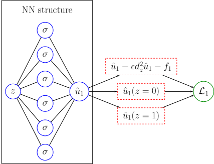
(a) traditional PINN for $u^{\varepsilon}_{1}$

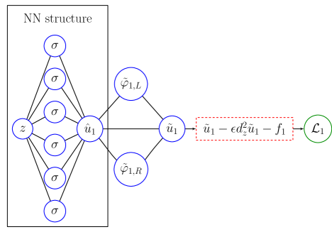
(b) sl-PINN for $u^{\varepsilon}_{1}$

Figure 3.1. Schematic difference between PINN and sl-PINN for $u_{1}^{\varepsilon}$.

3.2. sl-PINN predictions for $u_{2}^{\varepsilon}$

Here we construct our sl-PINN for the second component $u^{\varepsilon}_{2}$, solution of (1.2)₂.

Because the explicit expression of the corrector $\varphi_{2}$, defined in (2.12), is not available, we are no longer able to construct our (singular layer) PINN prediction of $u^{\varepsilon}_{2}$ as simple as that for $u^{\varepsilon}_{1}$ in (3.3). Instead, we train the viscous solution $u^{\varepsilon}_{2}$ and the corrector $\varphi_{2}$ at the same time. That is, we construct one neural network, in part to train $u^{\varepsilon}_{2}$ and also to train $\varphi_{2}$ as well, and hence they interact each other in the form,

$$\tilde{u}_{2}(x,z;\boldsymbol{\Theta}_{2})=\hat{u}_{2}(x,z;\boldsymbol{\theta}_{2})+\tilde{\varphi}_{2,L}(x,z;\boldsymbol{\theta}_{2,s,L})+\tilde{\varphi}_{2,R}(x,z;\boldsymbol{\theta}_{2,s,R}),$$ (3.7)

and

$$\vspace{1.5mm}\tilde{\varphi}_{2,L}(x,z;\boldsymbol{\theta}_{2},\boldsymbol{\theta}_{2,s,L}) =-\hat{u}_{2}(x,0;\boldsymbol{\theta}_{2})e^{-z/\sqrt{\varepsilon}}+ze^{-z/\sqrt{\varepsilon}}\hat{\varphi}_{2,L}(x,z;\boldsymbol{\theta}_{2,s,L}),$$ (3.8)

$$\tilde{\varphi}_{2,R}(x,z;\boldsymbol{\theta}_{2},\boldsymbol{\theta}_{2,s,R}) =-\hat{u}_{2}(x,1;\boldsymbol{\theta}_{2})e^{-(1-z)/\sqrt{\varepsilon}}+(1-z)e^{-(1-z)/\sqrt{\varepsilon}}\hat{\varphi}_{2,R}(x,z;\boldsymbol{\theta}_{2,s,R}),$$ (3.9)

where $\hat{u}_{2}$, $\hat{\varphi}_{2,L}$ and $\hat{\varphi}_{2,R}$ are the network outputs and $\boldsymbol{\Theta}_{2}=\{\boldsymbol{\theta}_{2},\boldsymbol{\theta}_{2,s,L},\boldsymbol{\theta}_{2,s,R}\}$ with $\boldsymbol{\theta}_{2}$, $\boldsymbol{\theta}_{2,s,L}$, and $\boldsymbol{\theta}_{2,s,R}$ are the unknown parameters of the outputs $\hat{u}_{2}$, $\hat{\varphi}_{2,L}$, and $\hat{\varphi}_{2,R}$ respectively. We refer readers to see the picture of NN structure in Figure 3.2 with a comparison to the conventional PINN structure.

As analyzed in (2.11); see [14, 11] as well, it is verified that $\varphi_{2,L}$ and $\varphi_{2,R}$ behave like exponentially decaying functions from the boundaries at $z=0$ and $z=1$ (at least in the $H^{k}$ sense for $k=0,1,2$). Using this property, we construct our sl-PINN predicted solutions for $\varphi_{2,L}$ and $\varphi_{2,R}$ in part by using the exponentially decaying functions with respect to the stretched variables $z/\sqrt{\varepsilon}$ and $(1-z)/\sqrt{\varepsilon}$; the first terms on the right-hand side of (3.8) and (3.9). In addition, in order to implement the (implicit) interaction between the correctors and the equation, we add the training parts in the structure, the second terms on on the right-hand side, in (3.8) and (3.9).

By our construction, the sl-PINN predictions of the correctors satisfies

• $\tilde{\varphi}_{2,L}=-\hat{u}_{2}$ at $z=0$ and $\tilde{\varphi}_{2,R}=-\hat{u}_{2}$ at $z=1$,

• $\tilde{\varphi}_{2,L}\to 0$ as $z\to\infty$ and $\tilde{\varphi}_{2,R}\to 0$ as $z\to-\infty$,

and hence we notice that

• $\tilde{u}_{2}=0$, up to an $e.s.t.$, at $z=0,1$.

Now, because the zero boundary condition is ensured in the structure of $\tilde{u}_{2}$ (up to an $e.s.t$), we define the loss function as

$$\begin{split}\mathcal{L}_{2}(\boldsymbol{\Theta}_{2};\mathcal{T}_{2},\mathcal{T}_{B})&=\frac{1}{|\mathcal{T}_{2}|}\sum_{(x,z)\in\mathcal{T}_{2}}\left|\tilde{u}_{2}-\varepsilon\Delta\tilde{u}_{2}+\tilde{u}_{1}\partial_{x}\tilde{u}_{2}-f_{2}\right|^{2}\\ &+\frac{1}{|\mathcal{T}_{B}|}\sum_{(x,z)\in\mathcal{T}_{B}}\left|\tilde{u}_{2}(x=0,z)-\tilde{u}_{2}(x=L,z)\right|^{2},\end{split}$$ (3.10)

where $\mathcal{T}_{2}$ is the training set chosen in the domain $\Omega$ and $\mathcal{T}_{B}$ is the training set chosen on the periodic boundary $\partial\Omega\setminus\Gamma$. Since there is no boundary layer occurring in $x$ direction, the periodic boundary condition is simply enforced by penalizing the equivalent in the second term of the loss function. It is straightforward (by direct computations with (3.7) - (3.9)) to verify that the loss function $\mathcal{L}_{2}$ defined in (3.10) is bounded as $\varepsilon\to 0$. Therefore, the training process is reliable enough to reach an expected minimizer. The numerical experiments can be found in the next subsection 3.3.

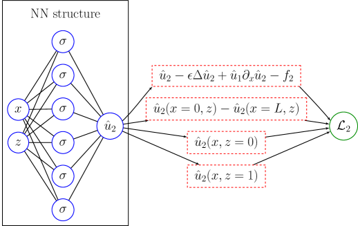
(a) traditional PINN for $u^{\varepsilon}_{2}$

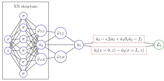
(b) sl-PINN for $u^{\varepsilon}_{2}$

Figure 3.2. Schematic difference between PINN and sl-PINN for $u_{2}^{\varepsilon}$.

3.3. Comparison between the conventional PINNs and the sl-PINNs for the velocity $\boldsymbol{u}^{\varepsilon}$

To examine the performance of the singular layer PINNs (sl-PINNs) enriched by the correctors, we introduce an exact solution $\boldsymbol{u}^{\varepsilon}$ for the problem (1.2) where the periodicity is set to be $L=1$ in the $x$-direction. By choosing the data $f_{1}(z)=1+z(1-z)$, we find the exact solution $u_{1}^{\varepsilon}$ as

$$u_{1}^{\varepsilon}(z)=(1-2\varepsilon)\left(1-\frac{1-e^{-\frac{1}{\sqrt{\varepsilon}}}}{1-e^{-\frac{2}{\sqrt{\varepsilon}}}}\left(e^{-\frac{z}{\sqrt{\varepsilon}}}+e^{-\frac{1-z}{\sqrt{\varepsilon}}}\right)\right).$$ (3.11)

By sequentially choosing the data $f_{2}$ as

$$f_{2}(x,z)=f_{1}(z)(1+\sin(2\pi x))+4\pi^{2}\varepsilon u_{1}^{\varepsilon}(z)\sin(2\pi x)+2\pi(u_{1}^{\varepsilon}(z))^{2}\cos(2\pi x),$$

we find that $u_{2}^{\varepsilon}$ as

$$u_{2}^{\varepsilon}(x,z)=u_{1}^{\varepsilon}(z)(1+\sin(2\pi x)).$$ (3.12)

We aim to verify the high-performance of our sl-PINNs for a small (but fixed) viscosity $0<\varepsilon\ll 1$ without excessive computational cost. Specifically, our goal is to sustain the efficiency of our learning method by preserving low computational costs while maintaining accurate approximations. To this end, we use two single-hidden-layer Neural Networks (NNs) with 20 neurons each to approximate $u_{1}^{\varepsilon}$ and $u_{2}^{\varepsilon}$ respectively. In addition, we select the number of training points $N=25$ uniformly distributed inside the domain $\Omega_{z}=[0,1]$ for training the loss $\mathcal{L}_{1}$ (3.6) and $N=50^{2}$ uniformly distributed inside the domain $\Omega=[0,1]\times[0,1]$ for training the loss $\mathcal{L}_{2}$ (3.10). The L-BFGS optimizer with learning rate $0.1$ is adopted to find a local minimum of $\mathcal{L}_{1}$ and $\mathcal{L}_{2}$ respectively. The maximum iteration is set as $50,000$, but the automatic termination is applied if tolerance is less than $10^{-8}$. In our experiments, we train the cases for $\varepsilon=10^{-3},10^{-4},10^{-5},10^{-6},10^{-7}$, and $10^{-8}$ with the same aforementioned settings. Five independent runs are conducted for each case to present the most accurate result. For the comparison, the conventional PINNs (PINNs) is also performed under the same settings for each case. We present here the loss values during the training process in Figures 3.3 and 3.4 for $\varepsilon=10^{-4}$, $10^{-6}$, and $10^{-8}$.

After completing the training process, we investigate the accuracy by plotting the testing points uniformly on the three locations in $z$ direction: $N_{test}=50$ points on the left boundary layer $\{z:0\leq z\leq\sqrt{\varepsilon}\}$, $N_{test}=50$ points on the right boundary layer $\{z:1-\sqrt{\varepsilon}\leq z\leq 1\}$ and $N_{test}=500$ points outside the boundary layer $\{z:\sqrt{\varepsilon}<z<1-\sqrt{\varepsilon}\}$. In the $x$-direction, $N_{test}=500$ testing points are simply drawn uniformly in $\{x:0\leq x\leq 1\}$. The results are shown in Tables 1 and 2 for approximating $u_{1}^{\varepsilon}$ and $u_{2}^{\varepsilon}$ respectively.

We observe that our sl-PINNs produce accurate predictions for every small viscosity $\varepsilon$, while the (usual) PINNs fail to predict the solution as the solution becomes stiffer. For in-depth understanding the solutions’ behavior, the profiles of the predicted solutions are shown in Figures 3.5 and 3.6 for $u_{1}^{\varepsilon}$ and in Figures 3.7 and 3.8 for $u_{2}^{\varepsilon}$. We notice that the smaller $\varepsilon>0$ gets, the more challenging it becomes for the PINNs to capture the (singular) behavior around the boundary layers. In contrast, the sl-PINNs predict well the (singular) solution for every small $\varepsilon$. Moreover, the training process of the sl-PINN is much faster than the PINN, as shown in the loss plots in Figures 3.3 and 3.4. These observations indicate that our sl-PINNs are not only accurate but also efficient for solving the stiff problems with a small viscosity $\varepsilon$.

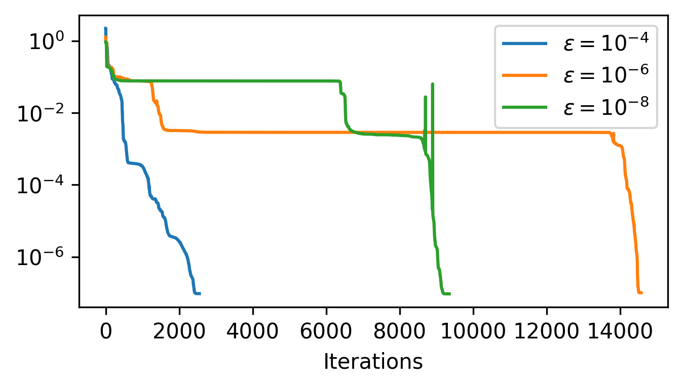
(a) PINNs

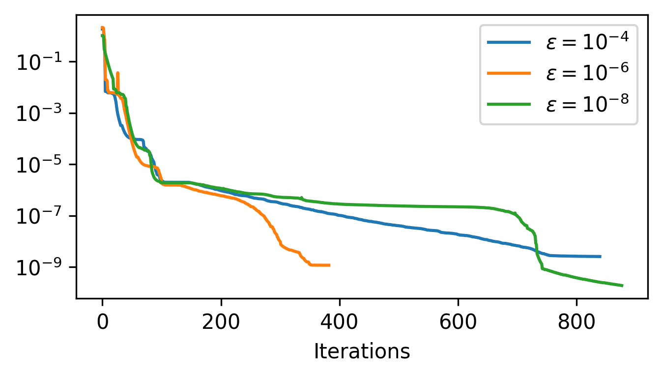
(b) sl-PINNs

Figure 3.3. The loss values during the training process for $u_{1}^{\varepsilon}$.

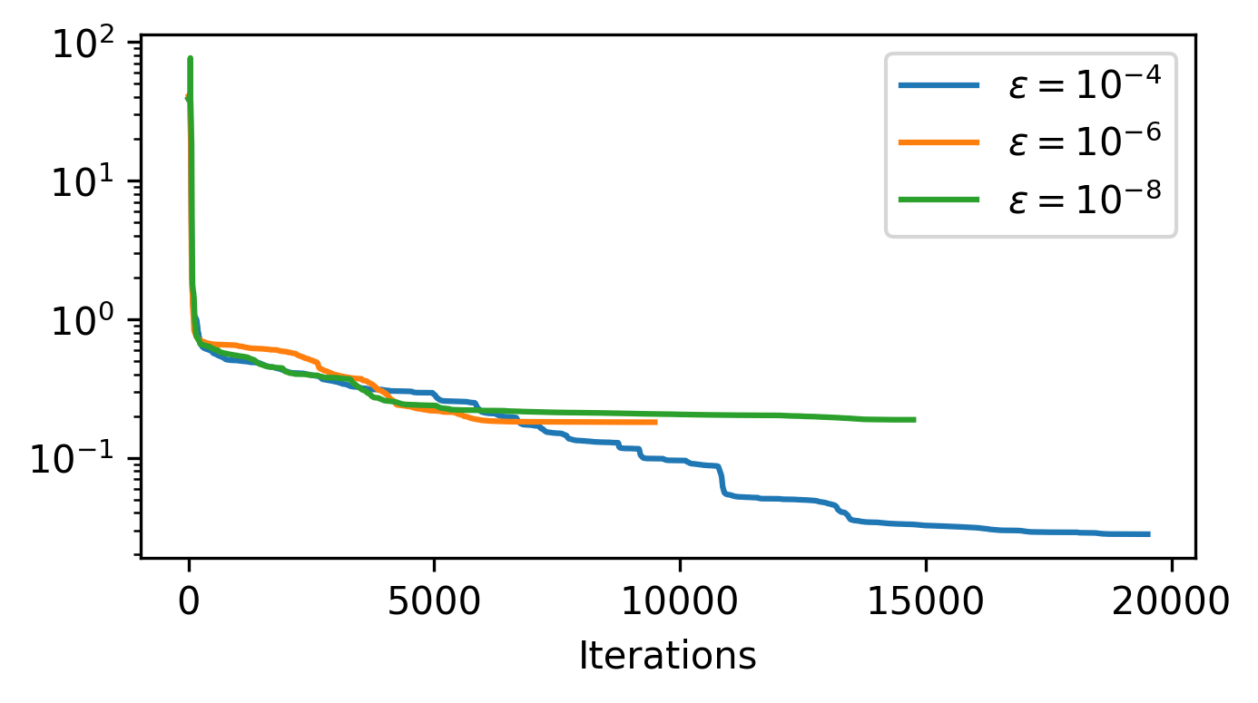
(a) PINNs

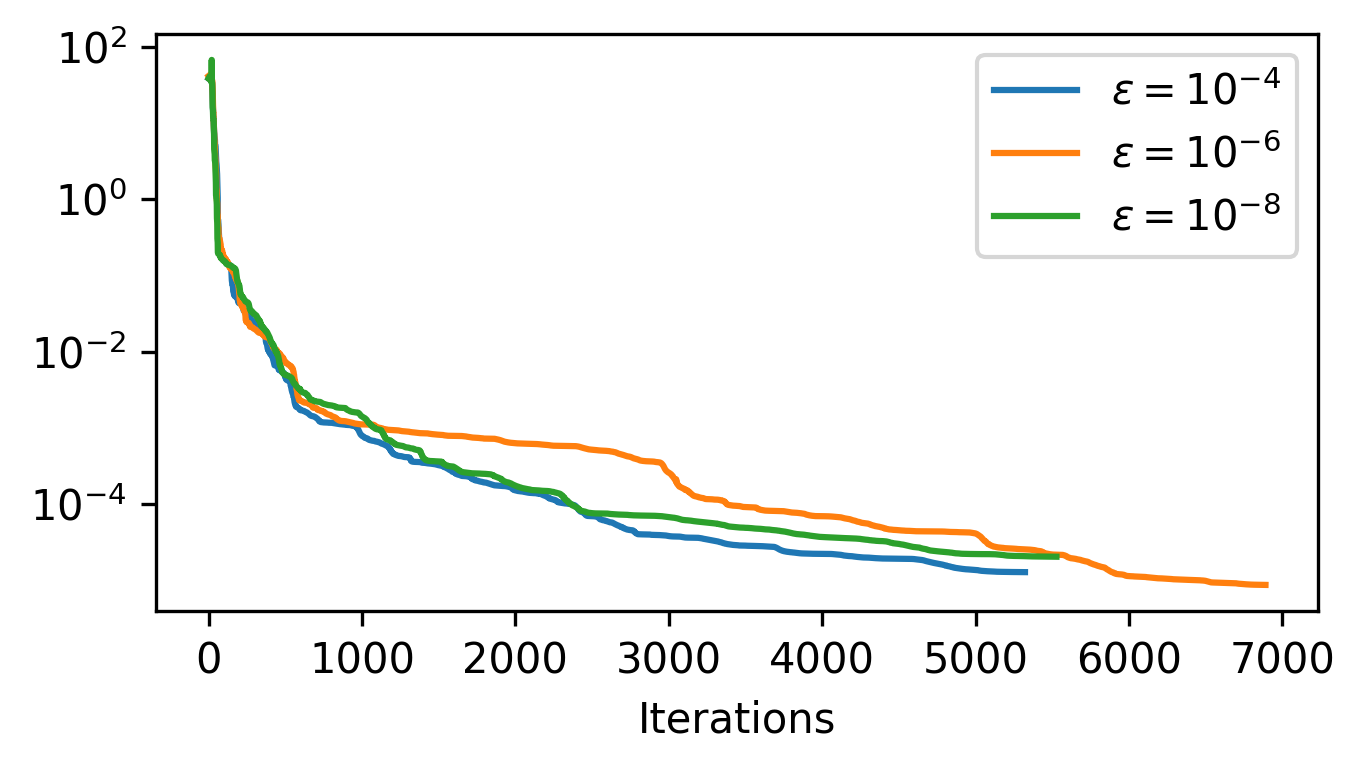
(b) sl-PINNs

Figure 3.4. The loss values during the training process for $u_{2}^{\varepsilon}$

	PINNs		sl-PINNs
	Relative $L^{2}$ error	Relative $L^{\infty}$ error	Relative $L^{2}$ error	Relative $L^{\infty}$ error
$\varepsilon=10^{-3}$	5.8741e-04	1.5534e-03	1.0452e-05	2.8015e-05
$\varepsilon=10^{-4}$	6.1017e-04	1.8356e-03	3.8054e-05	6.3043e-05
$\varepsilon=10^{-5}$	2.9297e-02	1.4135e-01	1.0672e-05	2.3559e-05
$\varepsilon=10^{-6}$	5.7345e-02	3.5576e-01	2.8798e-05	5.7216e-05
$\varepsilon=10^{-7}$	3.4765e-02	1.6841e-01	1.2835e-05	2.7431e-05
$\varepsilon=10^{-8}$	4.3961e-02	2.1925e-01	1.1757e-05	1.7917e-05

Table 1. Comparison between PINNs and sl-PINNs for $u_{1}^{\varepsilon}$.

	PINNs		sl-PINNs
	Relative $L^{2}$ error	Relative $L^{\infty}$ error	Relative $L^{2}$ error	Relative $L^{\infty}$ error
$\varepsilon=10^{-3}$	2.2551e-02	1.1572e-01	5.3896e-04	7.0597e-04
$\varepsilon=10^{-4}$	6.7786e-02	1.7088e-01	5.0758e-04	1.0775e-03
$\varepsilon=10^{-5}$	3.7465e-01	3.8308e+00	4.6892e-04	6.4305e-04
$\varepsilon=10^{-6}$	1.2475e-01	6.5216e-01	3.9502e-04	1.4244e-03
$\varepsilon=10^{-7}$	1.8177e-01	1.9354e+00	6.8371e-04	1.7341e-03
$\varepsilon=10^{-8}$	6.9807e+01	4.4609e+02	3.7568e-04	1.2459e-03

Table 2. Comparison between PINNs and sl-PINNs for $u_{2}^{\varepsilon}$.

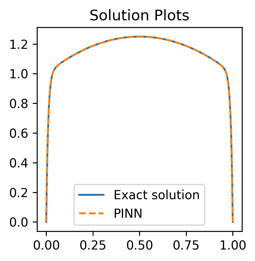
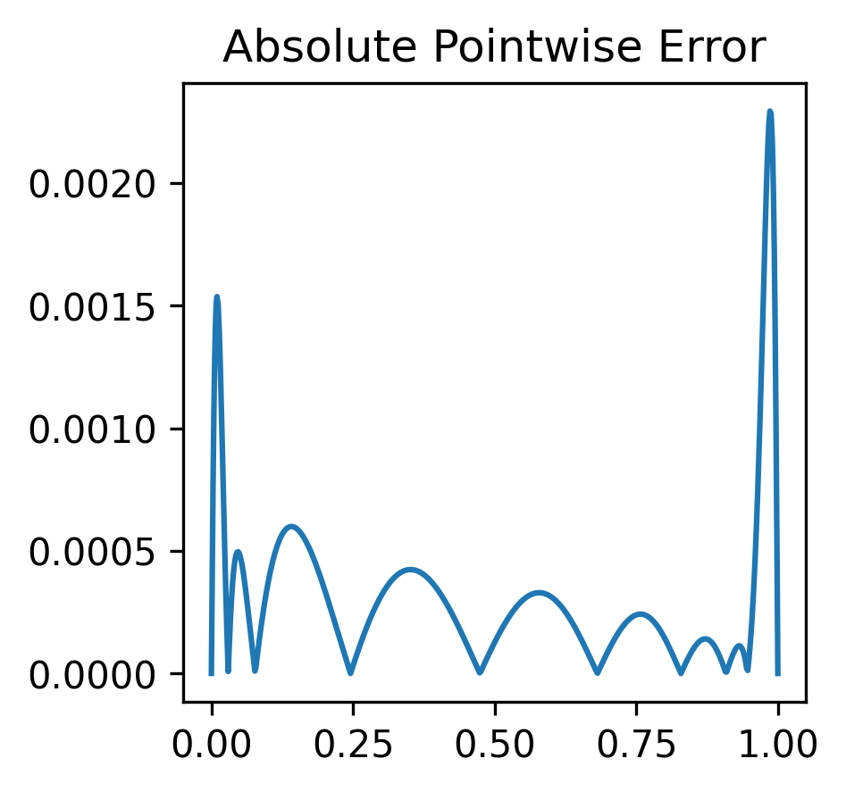
(a) $\varepsilon=10^{-4}$

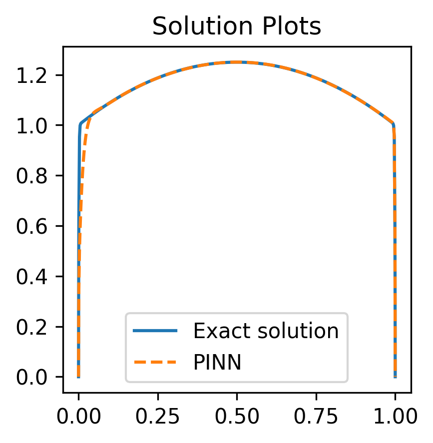
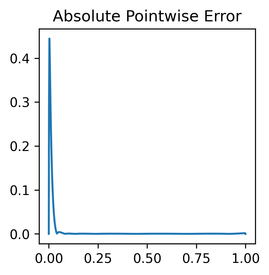
(b) $\varepsilon=10^{-6}$

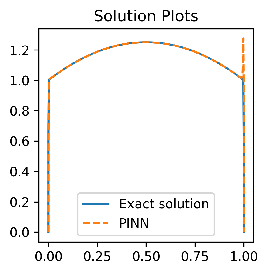
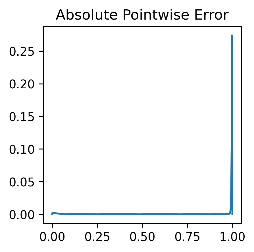
(c) $\varepsilon=10^{-8}$

Figure 3.5. Exact solutions and PINN predictions of $u_{1}^{\varepsilon}$.

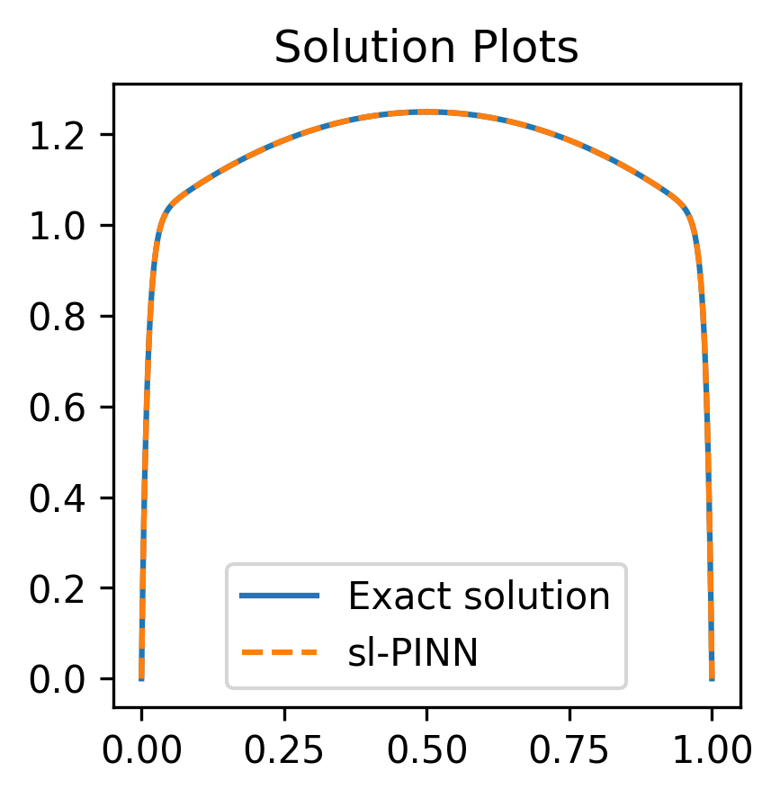
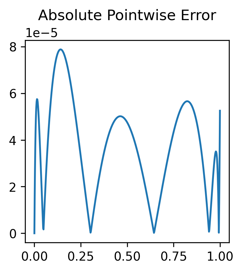
(a) $\varepsilon=10^{-4}$

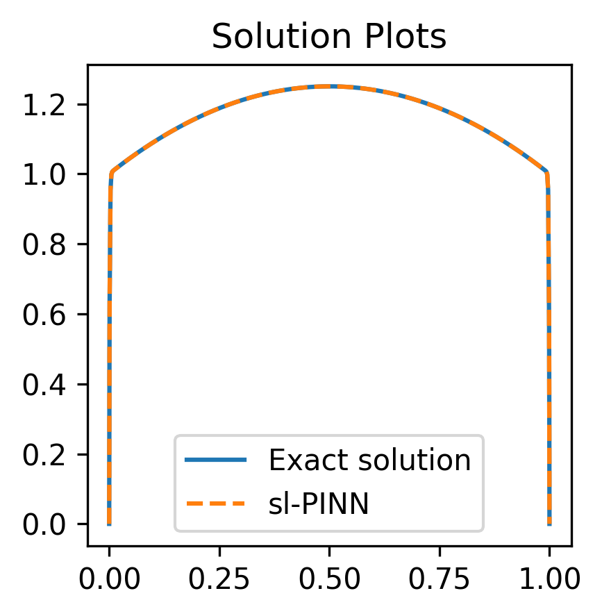
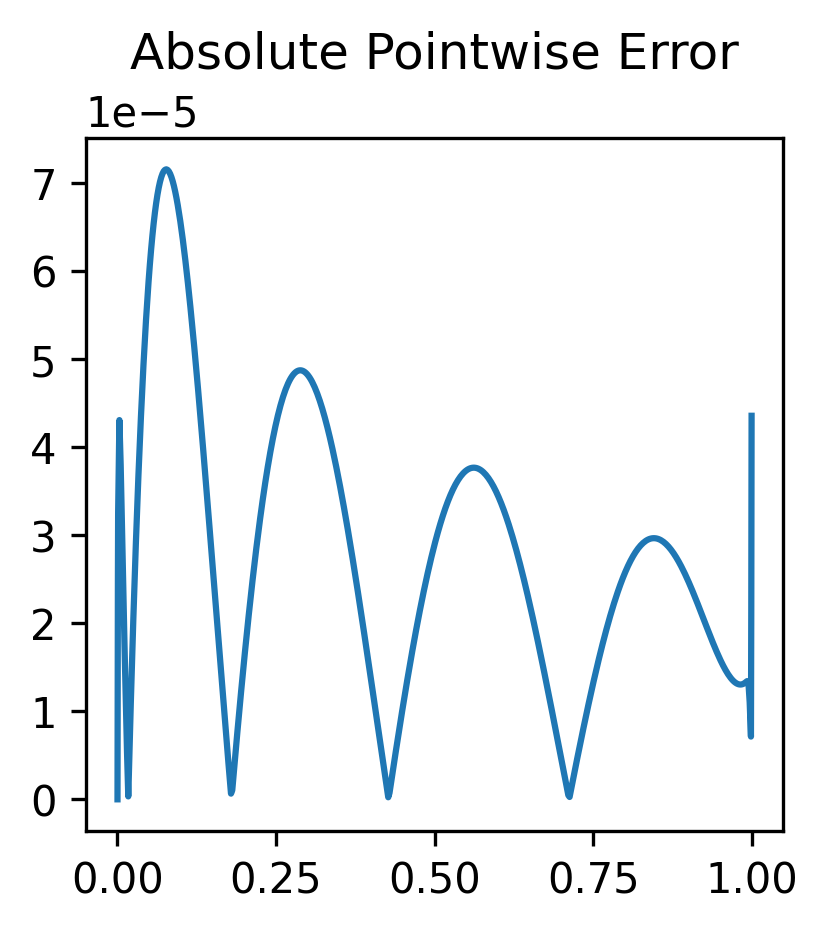
(b) $\varepsilon=10^{-6}$

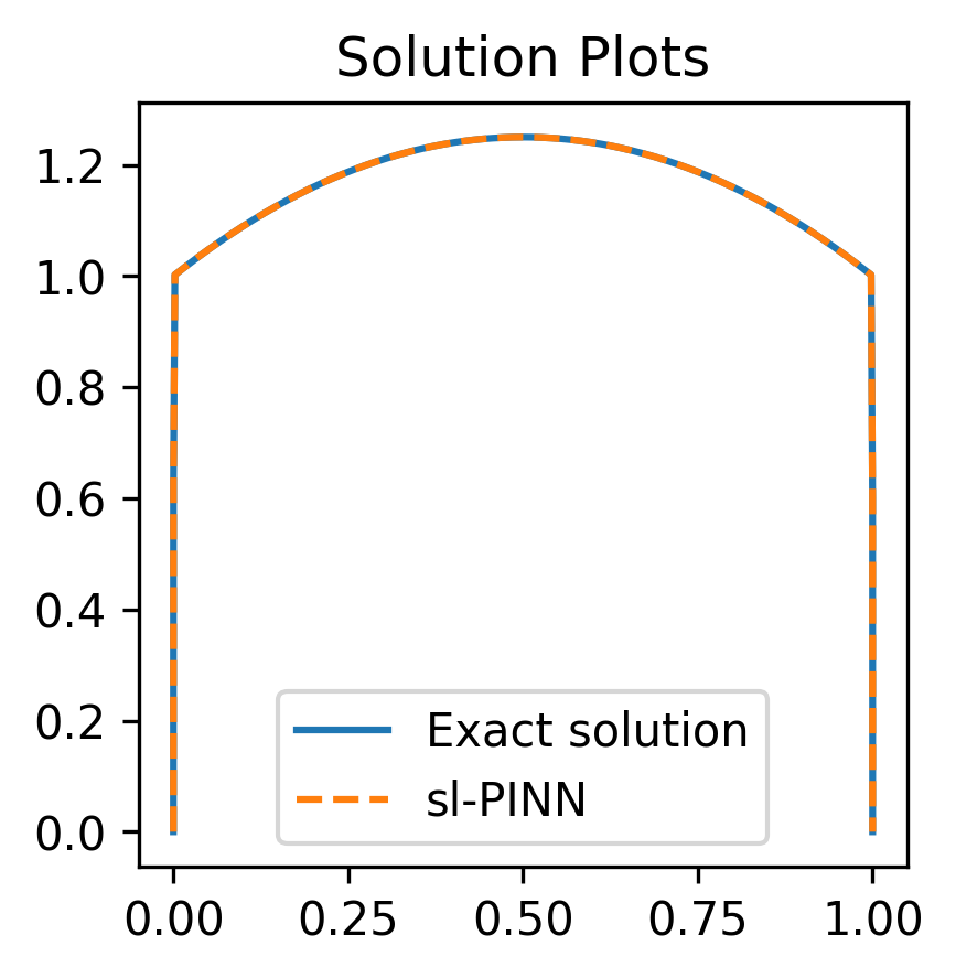
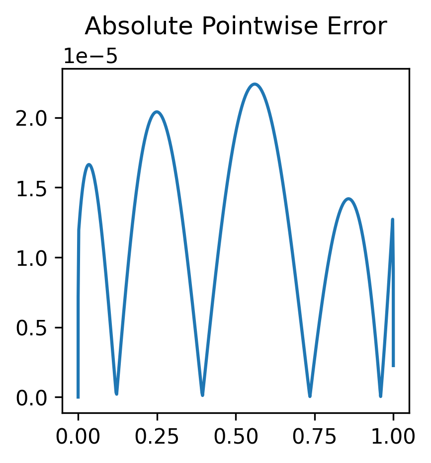
(c) $\varepsilon=10^{-8}$

Figure 3.6. Exact solutions and sl-PINN predictions of $u_{1}^{\varepsilon}$.

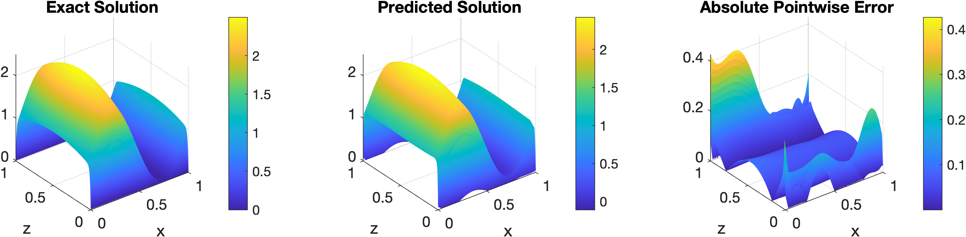
(a) $\varepsilon=10^{-4}$

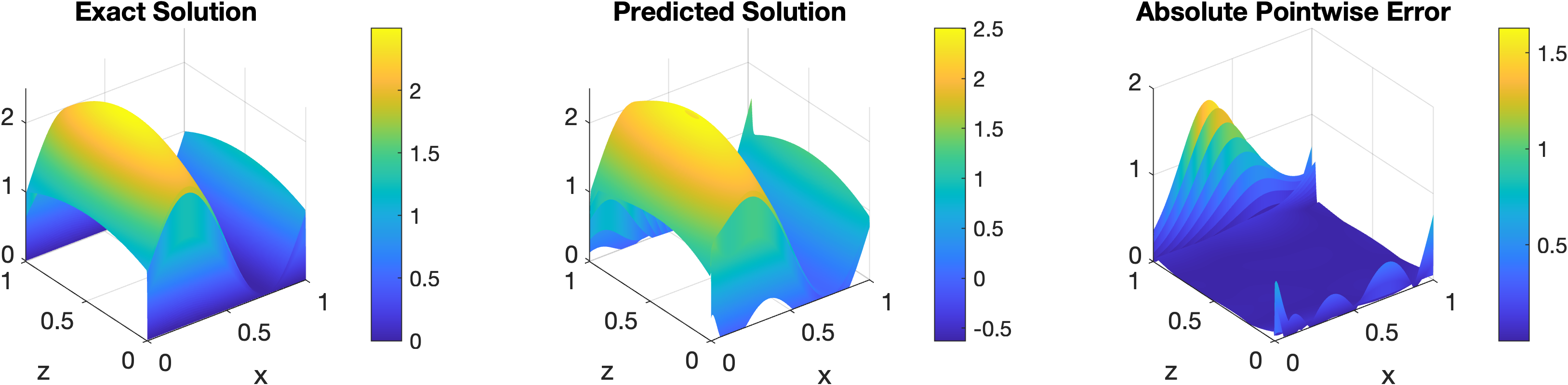
(b) $\varepsilon=10^{-6}$

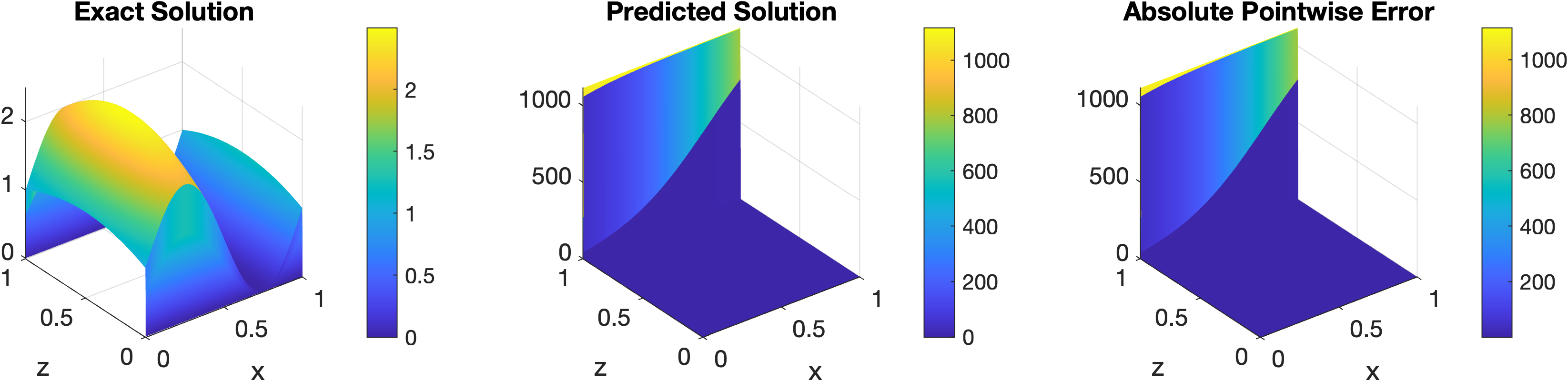
(c) $\varepsilon=10^{-8}$

Figure 3.7. Exact solutions and PINN predictions of $u_{2}^{\varepsilon}$.

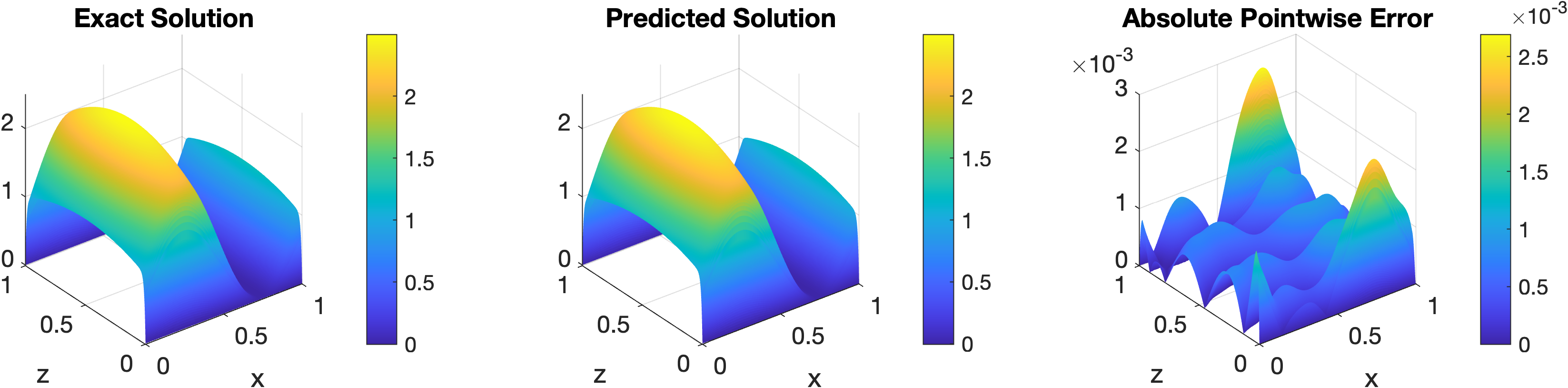
(a) $\varepsilon=10^{-4}$

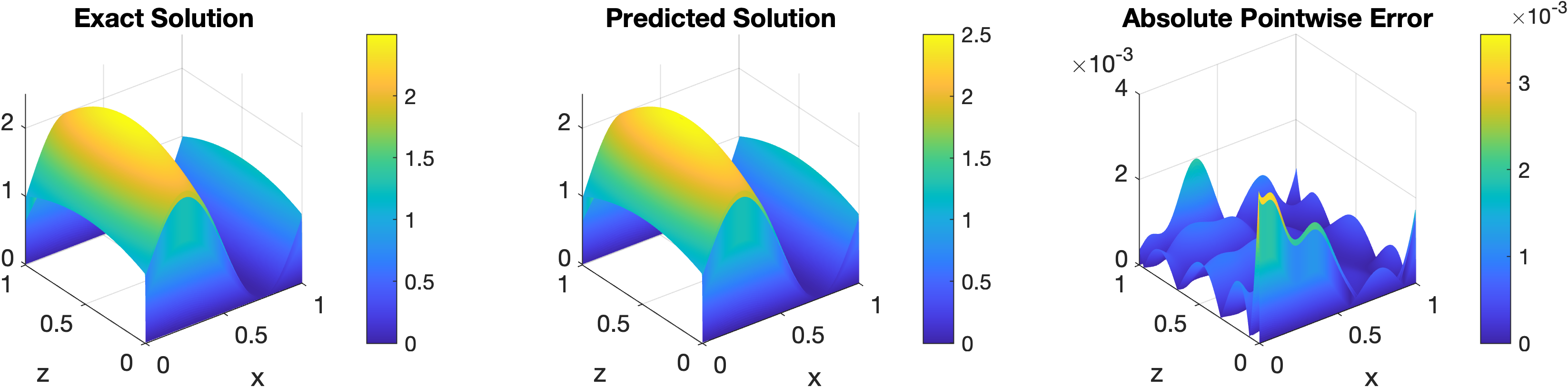
(b) $\varepsilon=10^{-6}$

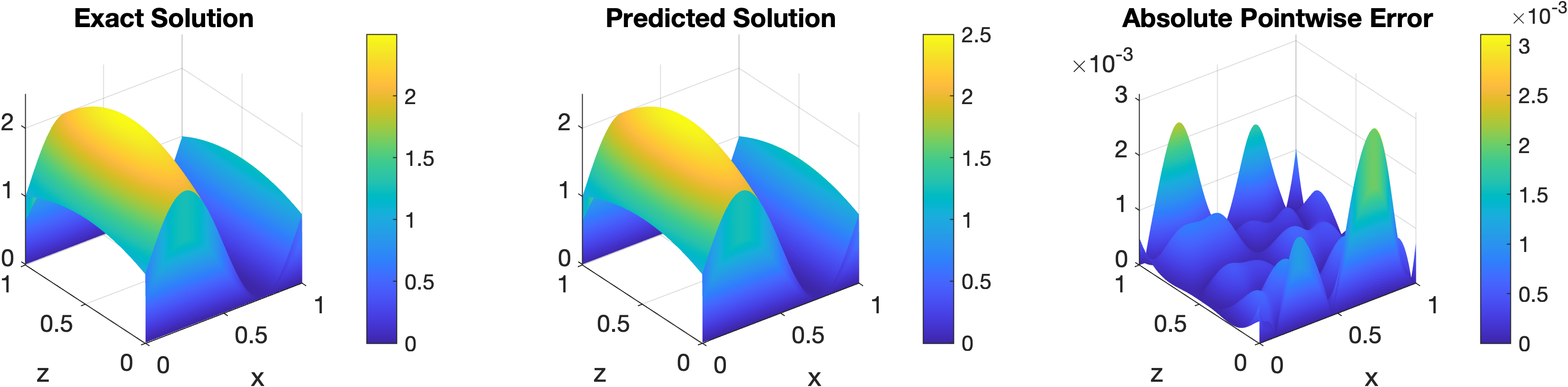
(c) $\varepsilon=10^{-8}$

Figure 3.8. Exact solutions and sl-PINN predictions of $u_{2}^{\varepsilon}$.

4. Numerical experiments for the vorticity

In this section, we present the framework and the experiments of our semi-analytic singular layer PINN (sl-PINN) methods for solving the vorticity equations (1.4), especially when the viscosity $\varepsilon$ is small.

Following the neural network (NN) architecture, introduced in Section 3, we recall the conventional PINN methods for the vorticity $\boldsymbol{\omega}^{\varepsilon}$ by constructing one network for each component of $\boldsymbol{\omega}^{\varepsilon}$. More precisely, we build a NN for $\omega^{\varepsilon}_{2}$ (sol. of (1.4)₂ with (1.5)₂) first. Then, using this predicted solution for $\omega^{\varepsilon}_{2}$ as well as the one for $u^{\varepsilon}_{1}$, built by the conventional PINN in the previous section 3, we construct the PINN predicted solution for $\omega^{\varepsilon}_{3}$ (sol. of (1.4)₃ with (1.5)₃), and, in a sequel, one for $\omega^{\varepsilon}_{1}$ (sol. of (1.4)₁ with (1.5)₁). We let $\hat{\omega}_{1}=\hat{\omega}_{1}(x,z;\boldsymbol{\theta}_{1})$, $\hat{\omega}_{2}=\hat{\omega}_{2}(z;\boldsymbol{\theta}_{2})$, and $\hat{\omega}_{3}=\hat{\omega}_{3}(x,z;\boldsymbol{\theta}_{3})$ denote the outputs of each NNs respectively where each $\boldsymbol{\theta}_{i}$ is the collection of the weights and bias for $\hat{\omega}_{i}$, $i=1,2,3$.

Using the equations and the boundary conditions in (1.4) - (1.5), we train the conventional PINN by minimizing the loss function, $\mathcal{L}_{i}$ for $\hat{\omega}_{i}$, $i=1,2,3$ below:

$$\mathcal{L}_{2}(\boldsymbol{\theta}_{2};\mathcal{T}_{2})=\frac{1}{|\mathcal{T}_{2}|}\sum_{z\in\mathcal{T}_{2}}\left|\hat{\omega}_{2}-\varepsilon d^{2}_{z}\hat{\omega}_{2}-d_{z}f_{1}\right|^{2}+\left|d_{z}\hat{\omega}_{2}(0)+\frac{1}{\varepsilon}f_{1}(0)\right|^{2}+\left|d_{z}\hat{\omega}_{2}(1)+\frac{1}{\varepsilon}f_{1}(1)\right|^{2},$$ (4.1)

where $\mathcal{T}_{2}\subset[0,1]$ is the set of training points,

$$\begin{split}\mathcal{L}_{3}(\boldsymbol{\theta}_{3};\mathcal{T}_{3},\mathcal{T}_{\Gamma},\mathcal{T}_{B})&=\frac{1}{|\mathcal{T}_{3}|}\sum_{(x,z)\in\mathcal{T}_{3}}\left|\hat{\omega}_{3}-\varepsilon\Delta\hat{\omega}_{3}+\hat{u}_{1}\partial_{x}\hat{\omega}_{3}-\partial_{x}f_{2}\right|^{2}\\ &+\frac{1}{|\mathcal{T}_{\Gamma}|}\sum_{(x,z)\in\mathcal{T}_{\Gamma}}\left|\hat{\omega}_{3}(x,z=0)\right|^{2}+\left|\hat{\omega}_{3}(x,z=1)\right|^{2}\\ &+\frac{1}{|\mathcal{T}_{B}|}\sum_{(x,z)\in\mathcal{T}_{B}}\left|\hat{\omega}_{3}(x=0,z)-\hat{\omega}_{3}(x=L,z)\right|^{2},\end{split}$$ (4.2)

where $\mathcal{T}_{3}\subset\Omega$, $\mathcal{T}_{\Gamma}\subset\Gamma$ and $\mathcal{T}_{B}\subset\partial\Omega\setminus\Gamma$ are the sets of training points, and

$$\begin{split}\mathcal{L}_{1}(\boldsymbol{\theta}_{1};\mathcal{T}_{1},\mathcal{T}_{\Gamma},\mathcal{T}_{B})&=\frac{1}{|\mathcal{T}_{1}|}\sum_{(x,z)\in\mathcal{T}_{1}}\left|\hat{\omega}_{1}-\varepsilon\Delta\hat{\omega}_{1}-\hat{\omega}_{2}\hat{\omega}_{3}+\hat{u}_{1}\partial_{x}\hat{\omega}_{1}+\partial_{z}f_{2}\right|^{2}\\ &+\frac{1}{|\mathcal{T}_{\Gamma}|}\sum_{(x,z)\in\mathcal{T}_{\Gamma}}\left|\partial_{z}\hat{\omega}_{1}(x,0)-\frac{1}{\varepsilon}f_{2}(x,0)\right|^{2}+\left|\partial_{z}\hat{\omega}_{1}(x,1)-\frac{1}{\varepsilon}f_{2}(x,1)\right|^{2}\\ &+\frac{1}{|\mathcal{T}_{B}|}\sum_{(x,z)\in\mathcal{T}_{B}}\left|\hat{\omega}_{1}(x=0,z)-\hat{\omega}_{1}(x=L,z)\right|^{2},\end{split}$$ (4.3)

where $\mathcal{T}_{1}\subset\Omega$ is the set of training points.

Notice that each of the loss functions $\mathcal{L}_{2}$ in (4.1) and $\mathcal{L}_{1}$ in (4.3) contains a term of order $\varepsilon^{-1}$, and hence they are not (expected to be) bounded uniformly in $\varepsilon$ as $\varepsilon\rightarrow 0$. In fact, because of this unbounded nature of the loss functions, the conventional PINN methods just fail to produce good predictions for the vorticity as we observe from the below numerical experiments in Section 4.2.

In the following section, we propose our new semi-analytic singular layer PINNs (sl-PINNs) to predict well the vorticity $\boldsymbol{\omega}^{\varepsilon}$. By embedding the singular profile of $\boldsymbol{\omega}^{\varepsilon}$ in the sl-PINNs structure, we build the corresponding NNs to train the smooth part of $\boldsymbol{\omega}^{\varepsilon}$ and finally obtain the accurate predicted solutions for $\boldsymbol{\omega}^{\varepsilon}$. As it appears in Section 4.1, our sl-PINNs produce accurate predictions for $\boldsymbol{\omega}^{\varepsilon}$ independent of a small $\varepsilon$.

4.1. sl-PINN predictions for the vorticity

To train predicted solutions for the vorticity $\boldsymbol{\omega}^{\varepsilon}=\text{curl }\boldsymbol{u}^{\varepsilon}=\big{(}-\partial_{z}u^{\varepsilon}_{2},\,d_{z}u^{\varepsilon}_{1},\,\partial_{x}u^{\varepsilon}_{2}\big{)}$ (sol. of (1.4) - (1.5)), we follow the methodology introduced in Sections 3.1 and 3.2 and construct our sl-PINNs sequentially for the components ${\omega}^{\varepsilon}_{2}$, ${\omega}^{\varepsilon}_{3}$, and then ${\omega}^{\varepsilon}_{1}$. In order to incorporate the singular behavior near the boundary of $\boldsymbol{\omega}^{\varepsilon}$ in our sl-PINN structure, we use below the profiles of the curl of the corrector $\tilde{\boldsymbol{\varphi}}_{*}=(\tilde{{\varphi}}_{1,*},\,\tilde{{\varphi}}_{2,*},\,0)$, $*=L,R$, defined in (3.4), (3.5), (3.8), and (3.9).

Note that the first component of the corrector $\tilde{{\varphi}}_{1,*}$, $*=L,R$, is given in its explicit form as in (3.4), (3.5), and hence we embed the $d_{z}\tilde{{\varphi}}_{1,*}$, $*=L,R$, in our sl-PINN structure for ${\omega}^{\varepsilon}_{2}$; see below in (4.4) and (4.5). On the other hand, because the explicit expression of second component $\tilde{{\varphi}}_{2,*}$, $*=L,R$, is not available, we train the viscous solution ${\omega}^{\varepsilon}_{3}$ (and then ${\omega}^{\varepsilon}_{1}$) together with training simultaneously the correctors $\partial_{x}\tilde{{\varphi}}_{2,*}$, $*=L,R$ (and then $-\partial_{z}\tilde{{\varphi}}_{2,*}$, $*=L,R$). This process is exactly what we employed for building our sl-PINN approximations for $u^{\varepsilon}_{2}$ in (3.7) - (3.9), but here we need to work with a different type of boundary condition, e.g., Neumann boundary condition for ${\omega}^{\varepsilon}_{1}$.

We introduce the sl-PINN predictions $\widetilde{\boldsymbol{\omega}}=(\widetilde{\omega}_{1},\widetilde{\omega}_{2},\widetilde{\omega}_{3})$ enriched by the correctors. For the $\tilde{\omega}_{2}$, using the fact that the corrector for $\omega^{\varepsilon}_{2}=d_{z}u^{\varepsilon}_{1}$ is $d_{z}\varphi_{1}$ and its explicit expression is available, i.e., $\varepsilon^{-1/2}e^{-z/\sqrt{\varepsilon}}$ near $z=0$, we write the sl-PINN structure as

$$\tilde{\omega}_{2}(z;\boldsymbol{\theta}_{2})=\hat{\omega}_{2}(z;\boldsymbol{\theta}_{2})+\tilde{\psi}_{2,L}(z;\boldsymbol{\theta}_{2})+\tilde{\psi}_{2,R}(z;\boldsymbol{\theta}_{2}),$$ (4.4)

where the correctors are defined by

$$\begin{cases}\vspace{1.5mm}\tilde{\psi}_{2,L}(z;\boldsymbol{\theta}_{2})=\displaystyle\big{(}f_{1}(0)+\varepsilon d_{z}\hat{\omega}_{2}(0;\boldsymbol{\theta}_{2})\big{)}\dfrac{1}{\sqrt{\varepsilon}}e^{-z/\sqrt{\varepsilon}},\\ \tilde{\psi}_{2,R}(z;\boldsymbol{\theta}_{2})=\displaystyle\big{(}-f_{1}(1)-{\varepsilon}d_{z}\hat{\omega}_{2}(1;\boldsymbol{\theta}_{2})\big{)}\dfrac{1}{\sqrt{\varepsilon}}e^{-(1-z)/\sqrt{\varepsilon}}.\end{cases}$$ (4.5)

Thanks to this setting of the correctors $\tilde{\psi}_{2,*}$, $*=L,R$, we notice that

• $\tilde{\psi}_{2,L}\to 0$ as $z\to\infty$ and $\tilde{\psi}_{2,R}\to 0$ as $z\to-\infty$,

• $d_{z}\tilde{\omega}_{2}=-\dfrac{1}{\varepsilon}f_{1}$, up to an $e.s.t.$, at $z=0,1$.

For the $\tilde{\omega}_{3}$, we use exactly the same construction as for the $u^{\varepsilon}_{2}$ in (3.7) - (3.9), and write

$$\tilde{\omega}_{3}(x,z;\boldsymbol{\Theta}_{3})=\hat{\omega}_{3}(x,z;\boldsymbol{\theta}_{3})+\tilde{\psi}_{3,L}(x,z;\boldsymbol{\theta}_{3},\boldsymbol{\theta}_{3,s,L})+\tilde{\psi}_{3,R}(x,z;\boldsymbol{\theta}_{3},\boldsymbol{\theta}_{3,s,R}),$$ (4.6)

with

$$\begin{cases}\vspace{1.5mm}\tilde{\psi}_{3,L}(x,z;\boldsymbol{\theta}_{3},\boldsymbol{\theta}_{3,s,L})=-\hat{\omega}_{3}(x,0;\boldsymbol{\theta}_{3})e^{-z/\sqrt{\varepsilon}}+ze^{-z/\sqrt{\varepsilon}}\hat{\psi}_{3,L}(x,z;\boldsymbol{\theta}_{3,s,L}),\\ \tilde{\psi}_{3,R}(x,z;\boldsymbol{\theta}_{3},\boldsymbol{\theta}_{3,s,R})=-\hat{\omega}_{3}(x,1;\boldsymbol{\theta}_{3})e^{-(1-z)/\sqrt{\varepsilon}}+(1-z)e^{-(1-z)/\sqrt{\varepsilon}}\hat{\psi}_{3,R}(x,z;\boldsymbol{\theta}_{3,s,R}).\end{cases}$$ (4.7)

That is, we use a neural network for training $\hat{\omega}_{3}$ and $\hat{\psi}_{3}$ at the same time. By our construction (and the analysis in (2.11)), we observe that

• $\tilde{\psi}_{3,L}\to 0$ as $z\to\infty$ and $\tilde{\psi}_{3,R}\to 0$ as $z\to-\infty$,

• $\tilde{\omega}_{3}=0$, up to an $e.s.t.$, at $z=0,1$.

For the first component $\tilde{\omega}_{1}$, we combine the methods we employed for the other two components $\tilde{\omega}_{2}$ and $\tilde{\omega}_{3}$. Namely, we write our sl-PINN structure for $\tilde{\omega}_{1}$ by training the $\hat{\omega}_{1}$ (smooth part) and the $\hat{\psi}_{1}$ (singular part) simultaneously and by enforcing the Neumann boundary condition, in the form,

$$\tilde{\omega}_{1}(x,z;\boldsymbol{\Theta}_{1})=\hat{\omega}_{1}(x,z;\boldsymbol{\theta}_{1})+\tilde{\psi}_{1,L}(x,z;\boldsymbol{\theta}_{1},\boldsymbol{\theta}_{1,s,L})+\tilde{\psi}_{1,R}(x,z;\boldsymbol{\theta}_{1},\boldsymbol{\theta}_{1,s,R}),$$ (4.8)

with

$$\begin{cases}\tilde{\psi}_{1,L}(x,z;\boldsymbol{\theta}_{1},\boldsymbol{\theta}_{1,s,L})=&\vspace{1.5mm}\Big{(}-f_{2}(x,0)+{\varepsilon}\partial_{z}\hat{\omega}_{1}(x,0;\boldsymbol{\theta}_{1})\Big{)}\dfrac{1}{\sqrt{\varepsilon}}e^{-z/\sqrt{\varepsilon}}\\ &\vspace{1.5mm}+z^{2}e^{-z/\sqrt{\varepsilon}}\hat{\psi}_{1,L}(x,z;\boldsymbol{\theta}_{1,s,L}),\\ \tilde{\psi}_{1,R}(x,z;\boldsymbol{\theta}_{1},\boldsymbol{\theta}_{1,s,R})=&\vspace{1.5mm}\Big{(}f_{2}(x,1)-{\varepsilon}\partial_{z}\hat{\omega}_{1}(x,1;\boldsymbol{\theta}_{1})\Big{)}\dfrac{1}{\sqrt{\varepsilon}}e^{-(1-z)/\sqrt{\varepsilon}}\\ &+(1-z)^{2}e^{-(1-z)/\sqrt{\varepsilon}}\hat{\psi}_{1,R}(x,z;\boldsymbol{\theta}_{1,s,R}).\end{cases}$$ (4.9)

We then observe that

• $\tilde{\psi}_{1,L}\to 0$ as $z\to\infty$ and $\tilde{\psi}_{1,R}\to 0$ as $z\to-\infty$,

• $\partial_{z}\tilde{\omega}_{1}=\dfrac{1}{\varepsilon}f_{2}$, up to an $e.s.t.$, at $z=0,1$.

In the constructions of $\tilde{\omega}_{i}$, $i=1,2,3,$ above, we used the notation for the learning parameters,

$$\boldsymbol{\Theta}_{i}=\{\boldsymbol{\theta}_{i},\,\boldsymbol{\theta}_{i,s,L},\,\boldsymbol{\theta}_{i,s,R}\},\quad i=1,2,3.$$ (4.10)

Because the boundary condition for $\tilde{\boldsymbol{\omega}}$ is already taken into account in the construction of our sl-PINNs, we define the loss functions for sl-PINNs as follows:

$$\mathcal{L}_{2}(\boldsymbol{\theta}_{2};\mathcal{T}_{2})=\frac{1}{|\mathcal{T}_{2}|}\sum_{z\in\mathcal{T}_{2}}\left|\tilde{\omega}_{2}-\varepsilon d^{2}_{z}\tilde{\omega}_{2}-d_{z}f_{1}\right|^{2},$$ (4.11)

where $\mathcal{T}_{2}\subset[0,1]$ is the set of training points,

$$\begin{split}\mathcal{L}_{3}(\boldsymbol{\Theta}_{3};\mathcal{T}_{3},\mathcal{T}_{\Gamma},\mathcal{T}_{B})&=\frac{1}{|\mathcal{T}_{3}|}\sum_{(x,z)\in\mathcal{T}_{3}}\left|\tilde{\omega}_{3}-\varepsilon\Delta\tilde{\omega}_{3}+\tilde{u}_{1}\partial_{x}\tilde{\omega}_{3}-\partial_{x}f_{2}\right|^{2}\\ &+\frac{1}{|\mathcal{T}_{B}|}\sum_{(x,z)\in\mathcal{T}_{B}}\left|\tilde{\omega}_{3}(x=0,z)-\tilde{\omega}_{3}(x=L,z)\right|^{2},\end{split}$$ (4.12)

where $\mathcal{T}_{3}\subset\Omega$, $\mathcal{T}_{\Gamma}\subset\Gamma$ and $\mathcal{T}_{B}\subset\partial\Omega\setminus\Gamma$ are the sets of training points, and

$$\begin{split}\mathcal{L}_{1}(\boldsymbol{\Theta}_{1};\mathcal{T}_{1},\mathcal{T}_{\Gamma},\mathcal{T}_{B})&=\frac{1}{|\mathcal{T}_{1}|}\sum_{(x,z)\in\mathcal{T}_{1}}\left|\tilde{\omega}_{1}-\varepsilon\Delta\tilde{\omega}_{1}-\tilde{\omega}_{2}\tilde{\omega}_{3}+\tilde{u}_{1}\partial_{x}\tilde{\omega}_{1}+\partial_{z}f_{2}\right|^{2}\\ &+\frac{1}{|\mathcal{T}_{B}|}\sum_{(x,z)\in\mathcal{T}_{B}}\left|\tilde{\omega}_{1}(x=0,z)-\tilde{\omega}_{1}(x=L,z)\right|^{2},\end{split}$$ (4.13)

where $\mathcal{T}_{1}\subset\Omega$ is the set of training points.

It is noteworthy to point out that the loss functions in (4.11), (4.12) and (4.13) stay bounded as the viscosity gets small, i.e., as $\varepsilon\to 0$. Thanks to this important feature, as we shall see below in Section 4.2, our sl-PINNs produce stable and accurate predictions for the vorticity, independent of the viscosity $\varepsilon$.

4.2. Comparison between the conventional PINNs and the sl-PINNs for the vorticity $\boldsymbol{\omega}^{\varepsilon}$

To perform the numerical experiments, we first write the exact solution for $\boldsymbol{\omega}^{\varepsilon}$ by taking curl of $\boldsymbol{u}^{\varepsilon}$ in (3.11) and (3.12):

$$\begin{cases}\vspace{1.5mm}\omega^{\varepsilon}_{1}(x,z)=-\omega^{\varepsilon}_{2}(z)(1+\sin(2\pi x)),\\ \vspace{1.5mm}\displaystyle\omega^{\varepsilon}_{2}(z)=-(1-2\varepsilon)\frac{1-e^{-\frac{1}{\sqrt{\varepsilon}}}}{1-e^{-\frac{2}{\sqrt{\varepsilon}}}}\left(\frac{-1}{\sqrt{\varepsilon}}e^{-\frac{z}{\sqrt{\varepsilon}}}+\frac{1}{\sqrt{\varepsilon}}e^{-\frac{1-z}{\sqrt{\varepsilon}}}\right)+1-2z,\\ \omega^{\varepsilon}_{3}(x,z)=2\pi u^{\varepsilon}_{1}(z)\cos(2\pi x).\end{cases}$$ (4.14)

We infer from (4.14) and the boundary layer analysis results in Theorem 1.1 that

• Asymptotic behavior of $\omega^{\varepsilon}_{3}$ is as much singular as that of $u^{\varepsilon}_{1}$ as $\varepsilon\rightarrow 0$. That is, as small as $e^{-\eta/\sqrt{\varepsilon}}$, $\eta=z$ or $1-z$, near the boundary.

• The $\omega^{\varepsilon}_{1}$ and $\omega^{\varepsilon}_{2}$ behave near the boundary as the approximation of identity, $\varepsilon^{-1/2}\,e^{-\eta/\sqrt{\varepsilon}}$, $\eta=z$ or $1-z$, which converges as $\varepsilon\rightarrow 0$ to a positive measure $\delta_{\Gamma}$ supported on the boundary $\Gamma$.

The asymptotic behavior at a small viscosity of the vorticity ($\omega^{\varepsilon}_{1}$ and $\omega^{\varepsilon}_{2}$) is more singular than that of the velocity vector field, and hence it is more challenging to approximate/predict the vorticity than the velocity at a small viscosity by employing PINN or any other classical numerical methods, e.g., Finite Elements, Finite Differences, Finite Volumes, or discontinuous Galerkin methods, and so on.

We aim to verify the accurate performance of our sl-PINN methods to approximate the solution $\boldsymbol{\omega}^{\varepsilon}$ to (1.4) without causing an excessive computation cost. The experimental settings are the same as those for the velocity in Section 3.3. We recall, in particular, that we use single-layer NNs with a small amount of training data to remain a low computational cost while maintaining sharp accuracy. The training data set $\mathcal{T}_{1}\subset\Omega$ for $\omega^{\varepsilon}_{1}$ is the same as $\mathcal{T}_{3}\subset\Omega$ for $\omega^{\varepsilon}_{3}$. The experiments for conventional PINNs are conducted for comparison with our sl-PINNs. We present here the results of $\omega^{\varepsilon}_{2}$ and $\omega^{\varepsilon}_{1}$ only since the equation for $\omega^{\varepsilon}_{3}$ is identical to that of $u^{\varepsilon}_{2}$, whose numerical simulations are well-studied in Section 3.3.

First, the loss value during the training process for $\omega^{\varepsilon}_{2}$ and $\omega^{\varepsilon}_{1}$ are shown in Figures 4.1 and 4.2 respectively. As expected, the conventional PINNs just fail to minimize the loss functions (4.1) and (4.3) because they started with an extremely large value in their minimization, results in an incorrect minimizer. On the contrary, our new sl-PINNs’ loss functions (4.11) and (4.13) are bounded independent of $\varepsilon$, and thus they are well minimized for every small $\varepsilon$. Moreover, the efficiency of sl-PINNs outperforms that of PINNs, as it reaches a minimum with far fewer iterations.

The computational errors are shown in Tables 3 and 4 for $\omega^{\varepsilon}_{2}$ and $\omega^{\varepsilon}_{1}$ respectively. The sl-PINNs obtain remarkable accuracy for every small $\varepsilon$, while the PINNs fail to approximate the solutions. More detailed information about the predicted solutions appear in Figures 4.3 and 4.4 for $\omega^{\varepsilon}_{2}$ and Figures 4.5 and 4.6 for $\omega^{\varepsilon}_{1}$. We conclude from the simulations that our sl-PINNs produce a sharp prediction of the vorticity at every small value of the viscosity $\varepsilon$, while the PINNs completely fail to predict the solution.

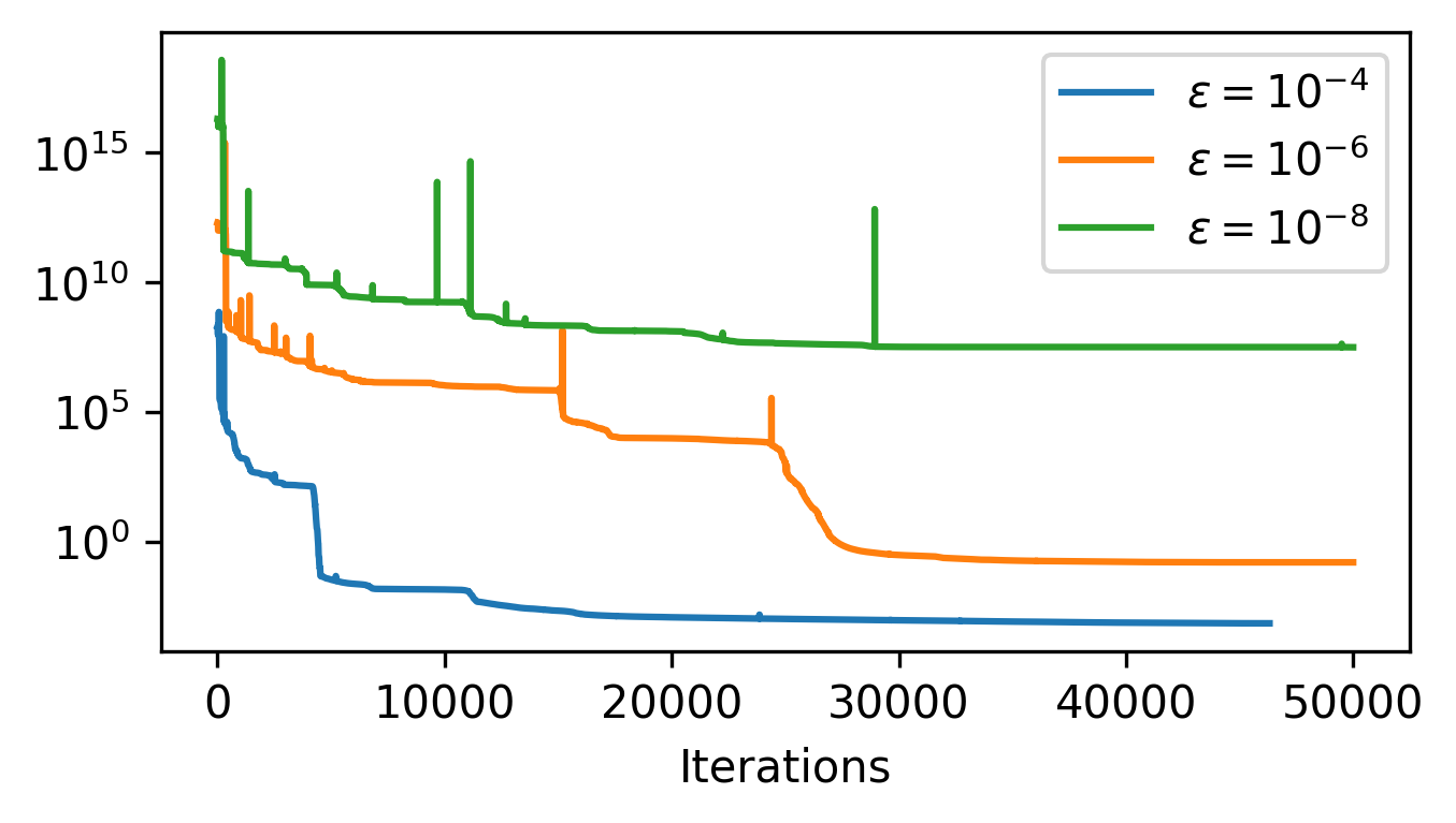
(a) PINNs

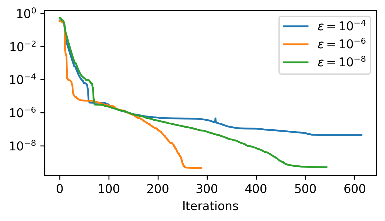
(b) sl-PINNs

Figure 4.1. The loss values during the training process for $\omega_{2}^{\varepsilon}$.

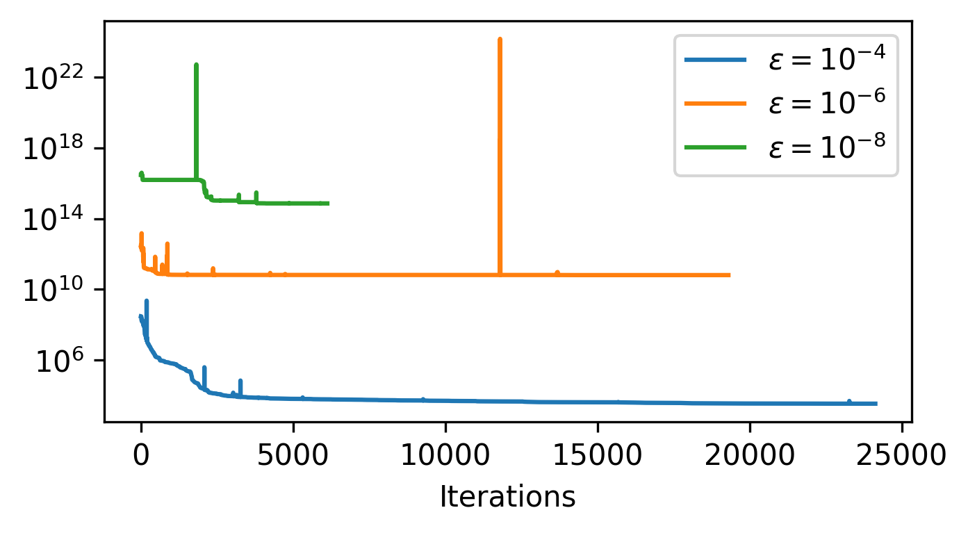
(a) PINNs

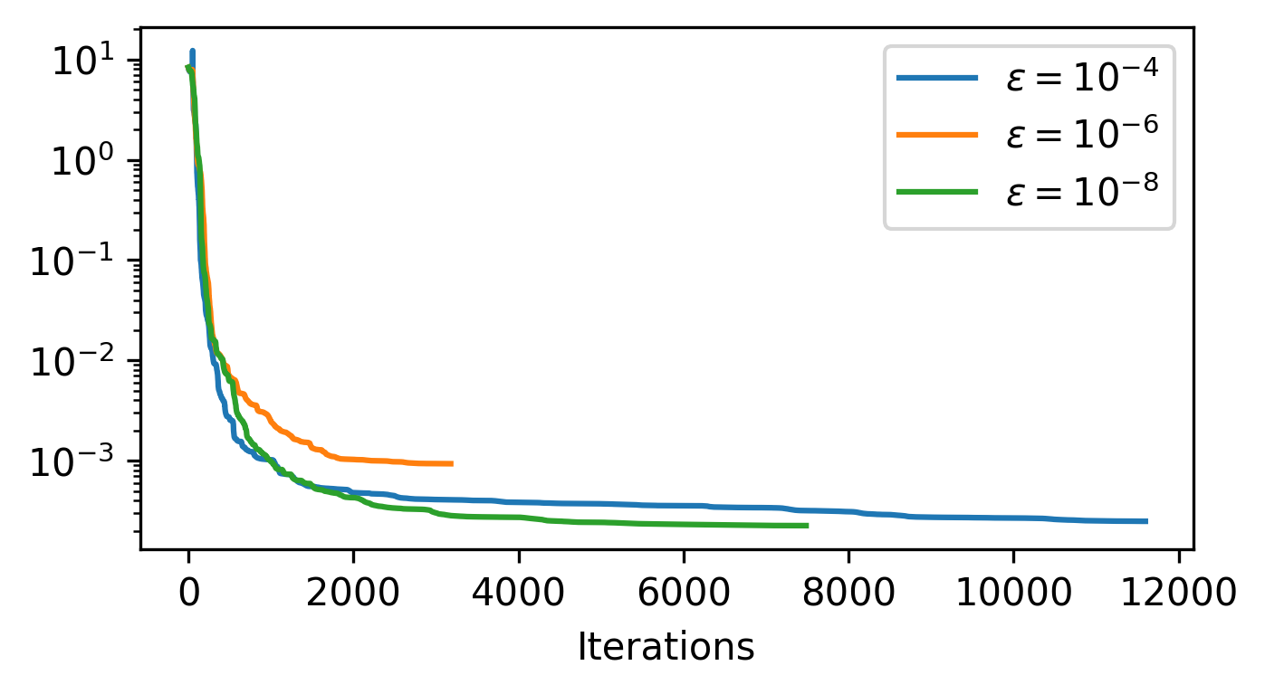
(b) sl-PINNs

Figure 4.2. The loss values during the training process for $\omega_{1}^{\varepsilon}$

	PINNs		sl-PINNs
	Relative $L^{2}$ error	Relative $L^{\infty}$ error	Relative $L^{2}$ error	Relative $L^{\infty}$ error
$\varepsilon=10^{-3}$	2.1347E-03	2.3484E-03	2.7971E-05	1.2545E-05
$\varepsilon=10^{-4}$	9.1606E-02	7.7010E-02	8.2069E-06	3.8037E-06
$\varepsilon=10^{-5}$	2.8411E-01	6.4230E-01	8.6951E-08	5.3314E-08
$\varepsilon=10^{-6}$	6.7560E-01	8.8517E-01	1.2268E-07	9.2237E-08
$\varepsilon=10^{-7}$	9.0956E-01	1.4045E+00	8.3588E-08	5.2581E-08
$\varepsilon=10^{-8}$	3.1965E+00	4.6734E+00	2.5566E-08	2.6715E-08

Table 3. Comparison between PINNs and sl-PINNs for $\omega_{2}^{\varepsilon}$.

	PINNs		sl-PINNs
	Relative $L^{2}$ error	Relative $L^{\infty}$ error	Relative $L^{2}$ error	Relative $L^{\infty}$ error
$\varepsilon=10^{-3}$	7.5808E-01	8.5224E-01	1.9381E-04	1.0485E-04
$\varepsilon=10^{-4}$	8.5395E-01	1.1084E+00	8.7578E-05	4.6931E-05
$\varepsilon=10^{-5}$	8.2919E-01	7.1802E-01	9.1033E-06	5.1658E-06
$\varepsilon=10^{-6}$	5.8776E+00	3.4830E+00	4.6694E-06	3.3595E-06
$\varepsilon=10^{-7}$	1.3017E+02	4.2646E+01	3.1714E-06	2.6672E-06
$\varepsilon=10^{-8}$	1.2058E+01	6.2136E+00	2.8830E-07	2.2172E-07

Table 4. Comparison between PINNs and sl-PINNs for $\omega_{1}^{\varepsilon}$.

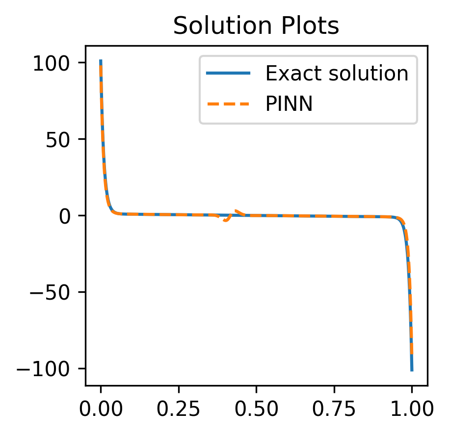
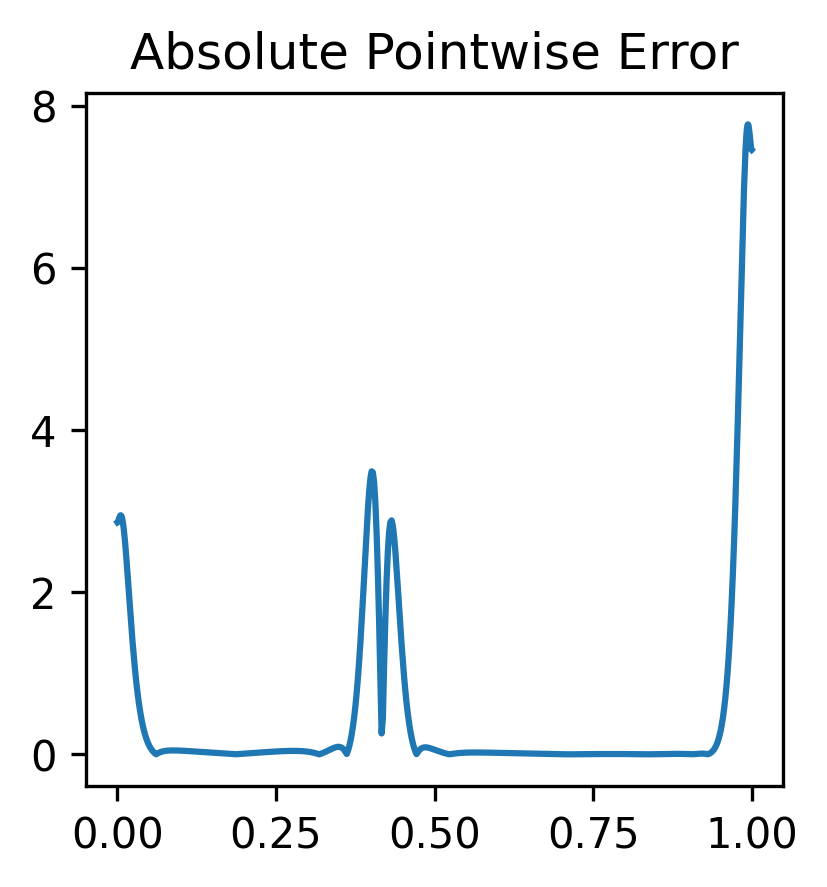
(a) $\varepsilon=10^{-4}$

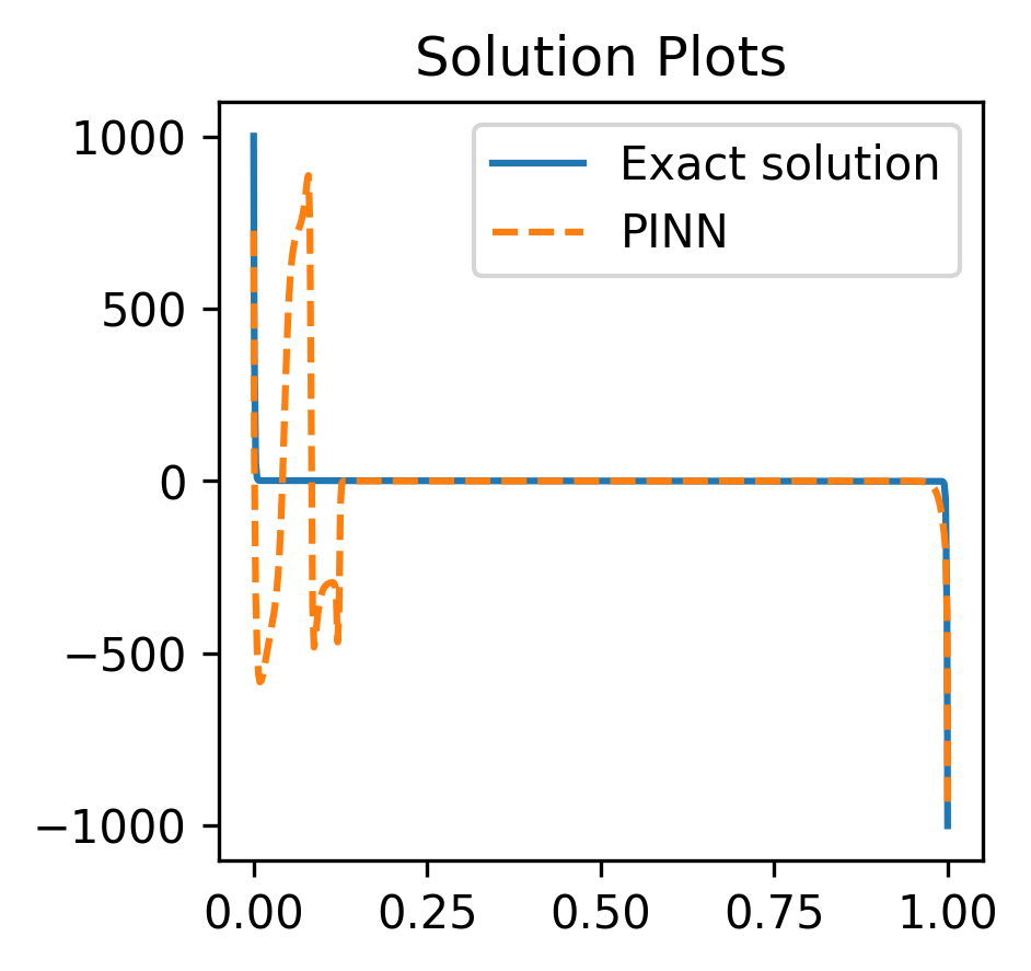
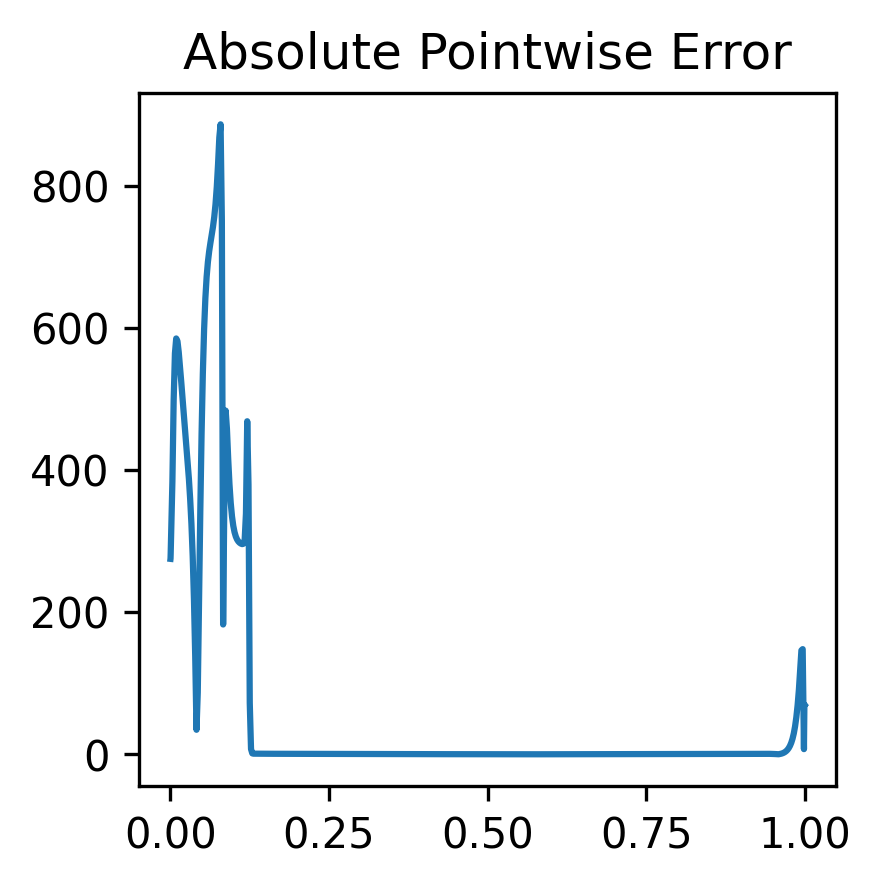
(b) $\varepsilon=10^{-6}$

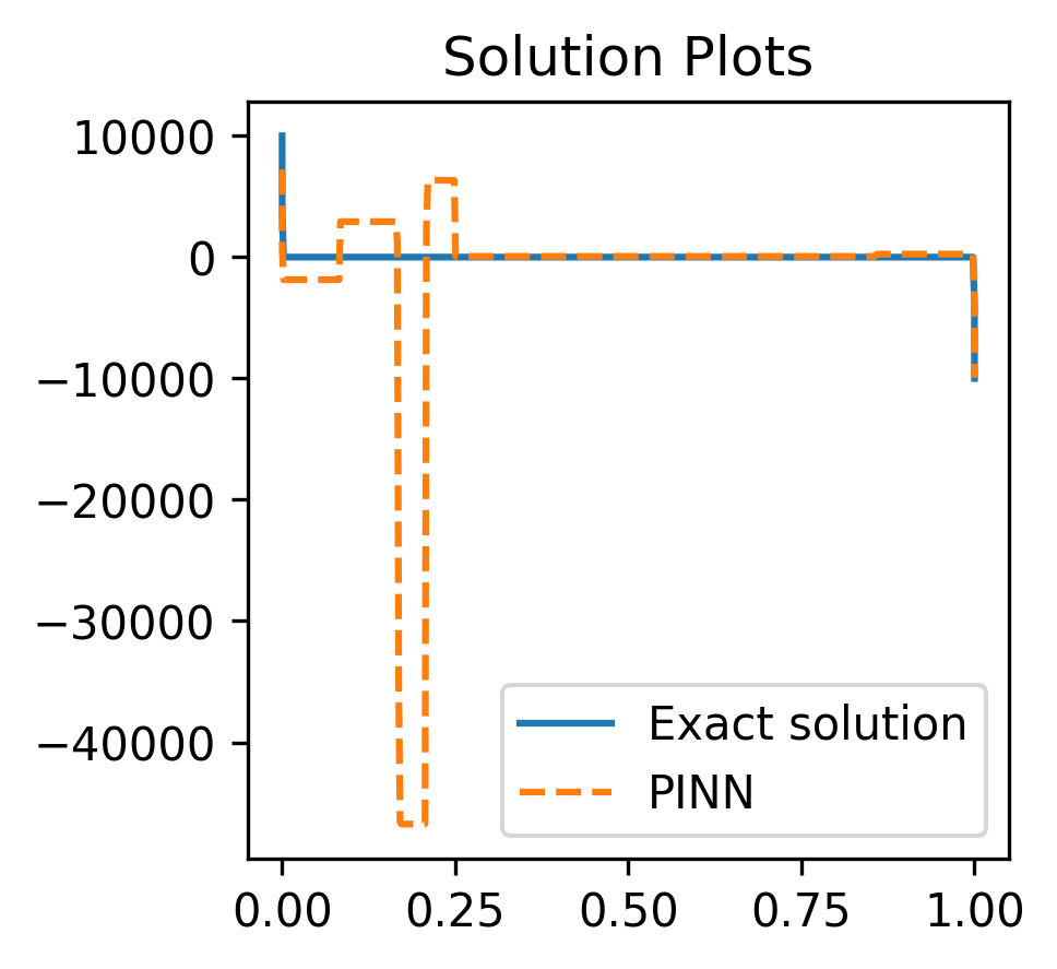
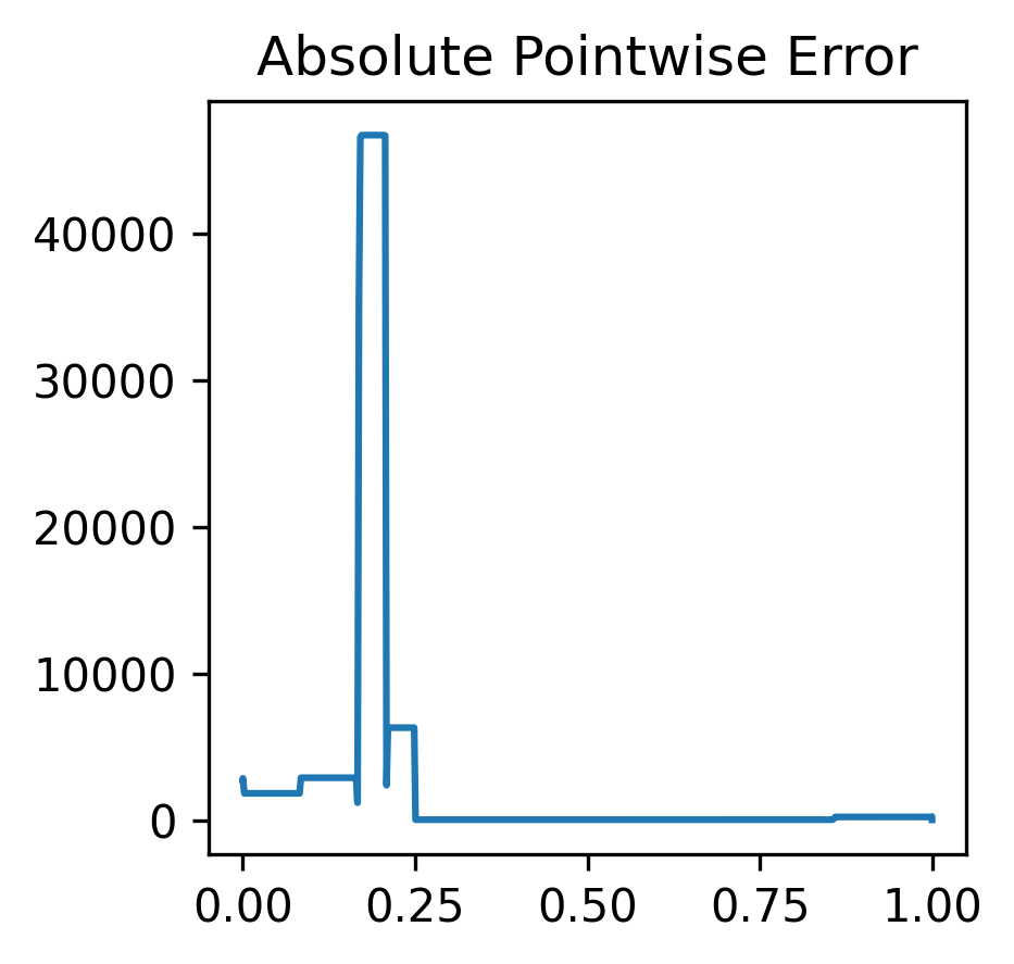
(c) $\varepsilon=10^{-8}$

Figure 4.3. Exact solutions and PINN predictions of $\omega_{2}^{\varepsilon}$.

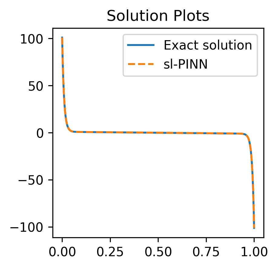
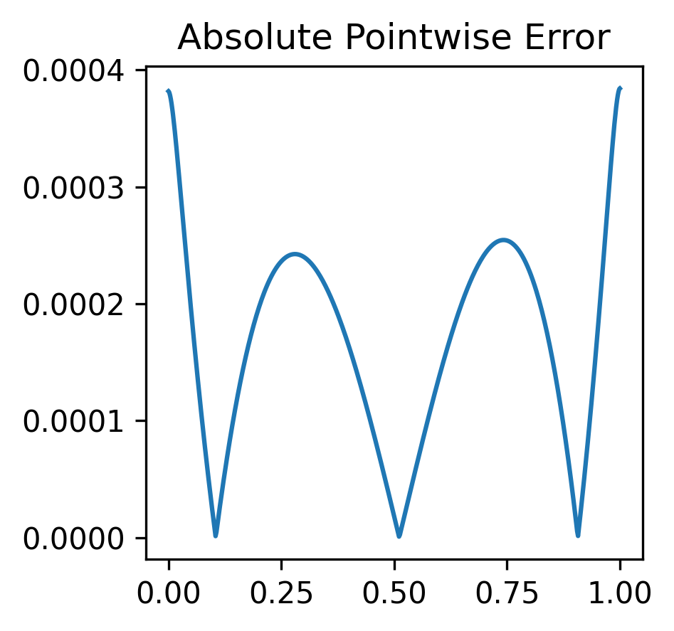
(a) $\varepsilon=10^{-4}$

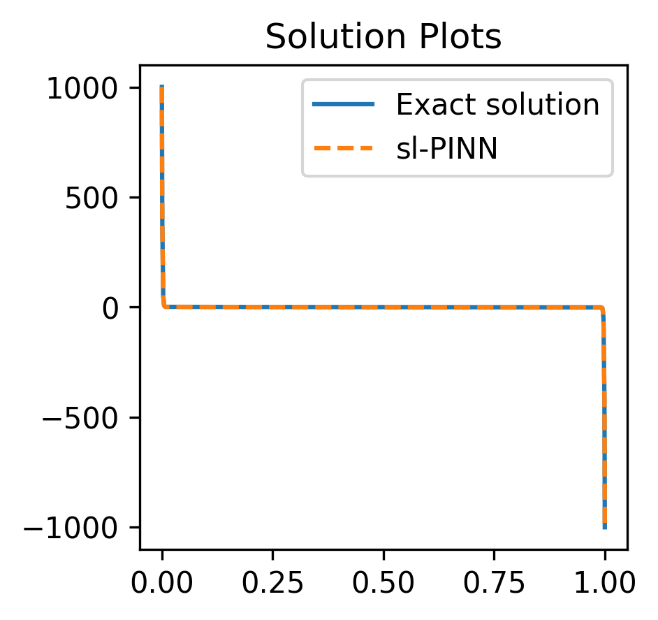
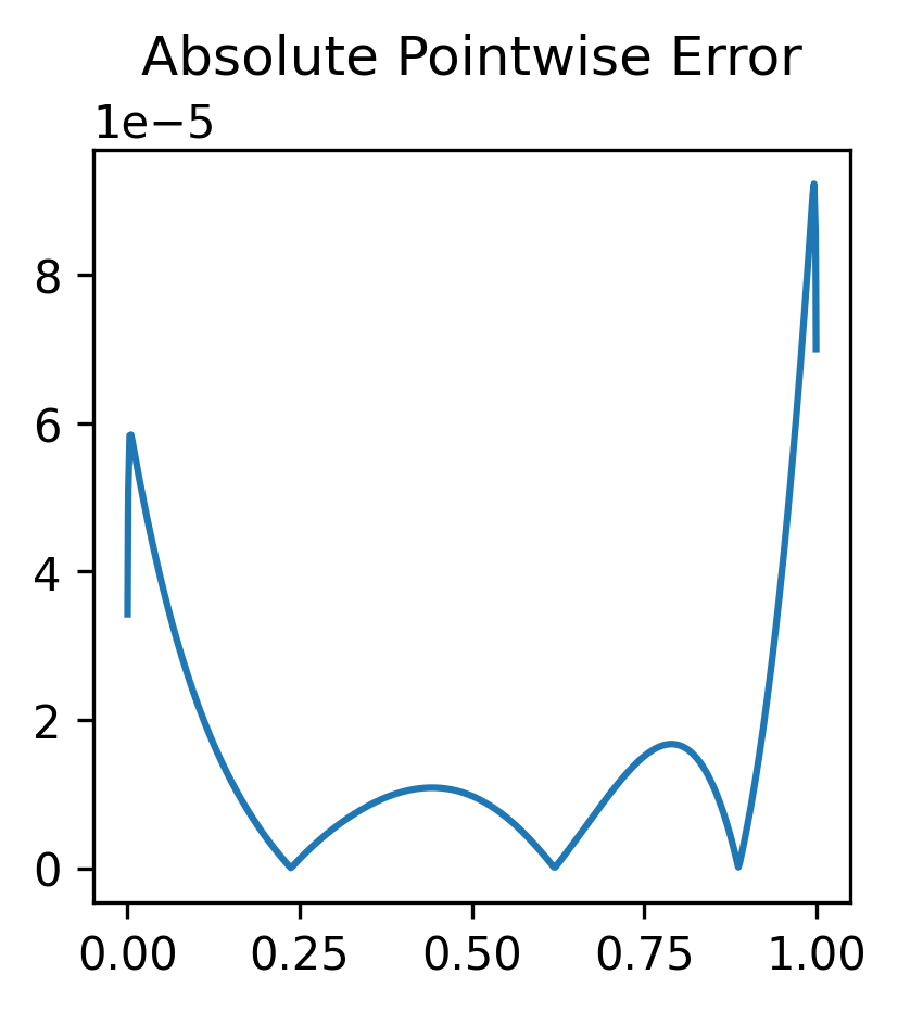
(b) $\varepsilon=10^{-6}$

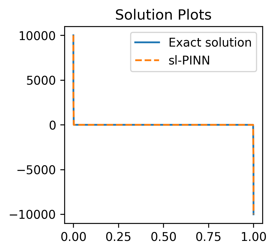
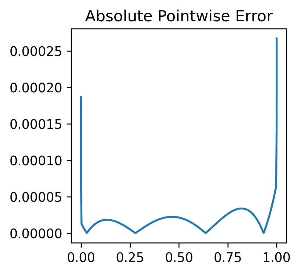
(c) $\varepsilon=10^{-8}$

Figure 4.4. Exact solutions and sl-PINNs predictins of $\omega_{2}^{\varepsilon}$.

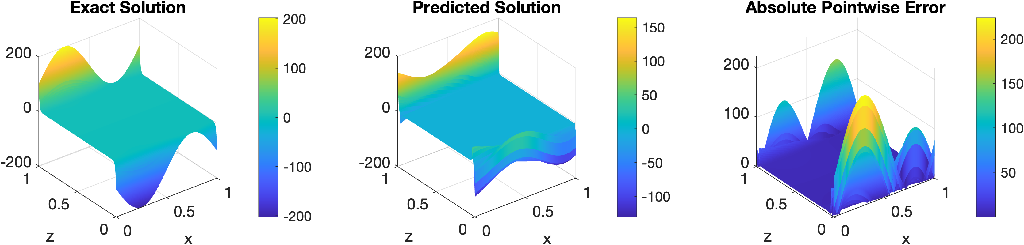
(a) $\varepsilon=10^{-4}$

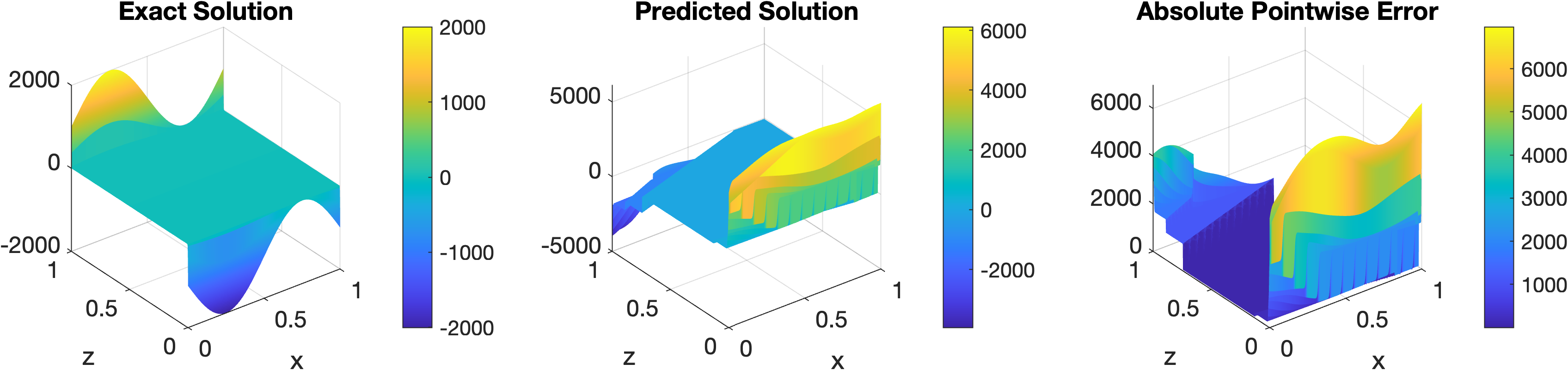
(b) $\varepsilon=10^{-6}$

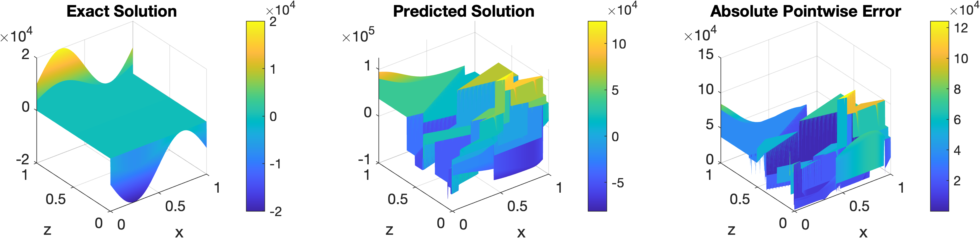
(c) $\varepsilon=10^{-8}$

Figure 4.5. Exact solutions and PINN predictins of $\omega_{1}^{\varepsilon}$.

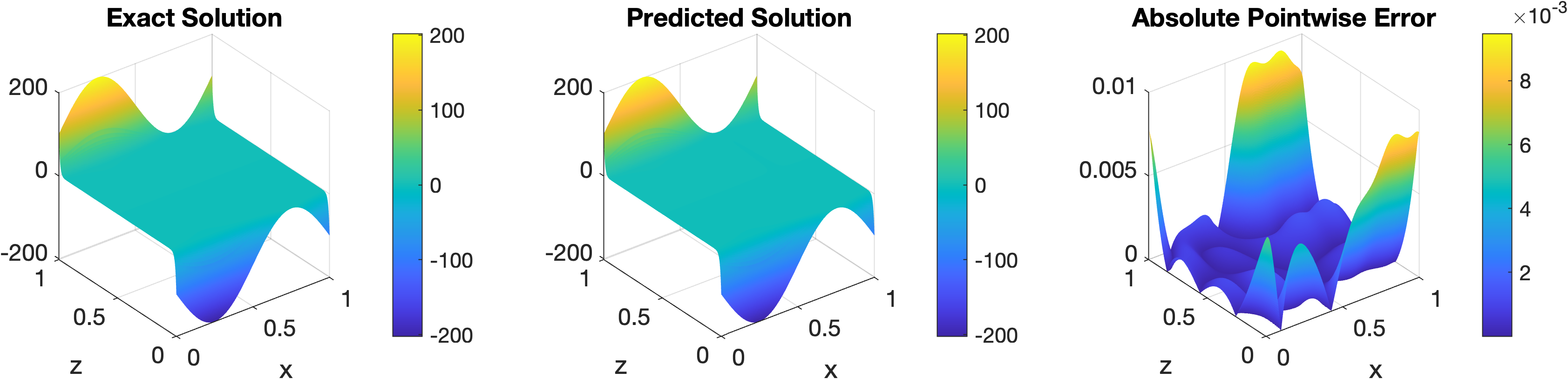
(a) $\varepsilon=10^{-4}$

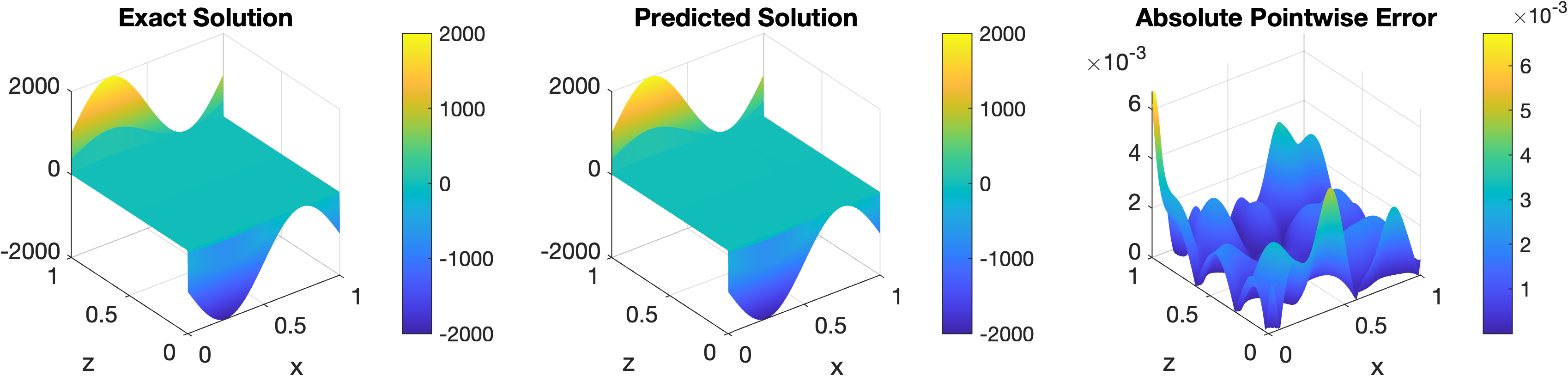
(b) $\varepsilon=10^{-6}$

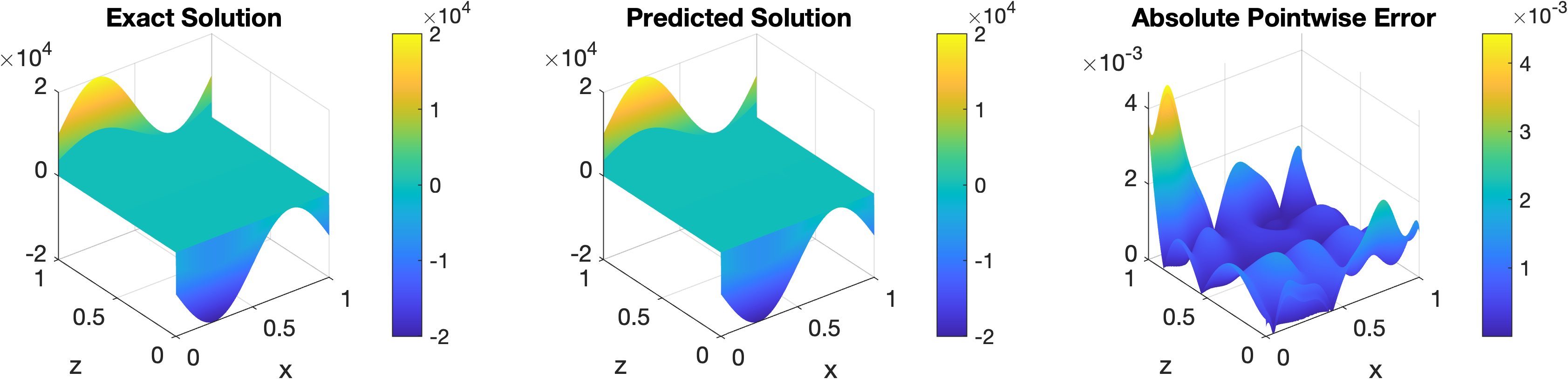
(c) $\varepsilon=10^{-8}$

Figure 4.6. Exact solutions and sl-PINNs predictins of $\omega_{1}^{\varepsilon}$.

References

[1]
Arzani, Amirhossein; Cassel, Kevin W.; D’Souza, Roshan M.
Theory-guided physics-informed neural networks for boundary layer problems with singular perturbation.
J. Comput. Phys. 473 (2023), Paper No. 111768, 15 pp.
[2]
Hassan Bararnia and Mehdi Esmaeilpour.
On the application of physics informed neural networks (PINN) to solve boundary layer thermal-fluid problems.
International Communications in Heat and Mass Transfer, 132:105890, 2022.
[4]
Félix Fernández de la Mata and Alfonso Gijón and Miguel Molina-Solana and Juan Gómez-Romero.
Physics-informed neural networks for data-driven simulation: Advantages, limitations, and opportunities.
Physica A: Statistical Mechanics and its Applications. 610:128415, 2023.
[5]
Mario De Florio, Enrico Schiassi, and Roberto Furfaro.
Physics-informed neural networks and functional interpolation for stiff chemical kinetics.
Chaos 32, 063107 (2022).
[6]
Olga Fuks and Hamdi A Tchelepi.
Limitations of physics informed machine learning for nonlinear two-phase
transport in porous media.
Journal of Machine Learning for Modeling and Computing, 1(1), 2020.
[7]
G.-M. Gie, Y. Hong, C.-Y. Jung, and D. Lee. Semi-analytic physics informed
neural network for convection-dominated boundary layer problems in 2D.
Submitted
[8]
G.-M. Gie, Y. Hong, C.-Y. Jung, and T. Munkhjin, Semi-analytic PINN methods for boundary layer problems in a rectangular domain.
Submitted.
[9]
G.-M. Gie, Y. Hong, and C.-Y. Jung.
Semi-analytic PINN methods for singularly perturbed boundary value problems
Submitted.
[10]
G.-M. Gie, C.-Y. Jung, and H. Lee.
Enriched Finite Volume approximations of the plane-parallel flow at a small viscosity.
Journal of Scientific Computing, 84, 7 (2020).
[11]
G.-M. Gie, C.-Y. Jung, and H. Lee.
Semi-analytic time differencing methods for singularly perturbed initial value problems.
Numerical Methods for Partial Differential Equations,
38, 5,
1367 - 139, 2022.
[12]
G.-M. Gie, C.-Y. Jung, and H. Lee.
Semi-analytic shooting methods for Burgers’ equation.
Journal of Computational and Applied Mathematics.
Vol. 418, 2023, 114694
[13]
G.-M. Gie, M. Hamouda, C.-Y. Jung, and R. Temam,
Singular perturbations and boundary layers, volume 200 of Applied Mathematical Sciences.
Springer Nature Switzerland AG, 2018.
https://doi.org/10.1007/978-3-030-00638-9
[14]
Gung-Min Gie, James P. Kelliher, Milton C. Lopes Filho, Anna L. Mazzucato, Helena J. Nussenzveig Lopes.
The vanishing viscosity limit for some symmetric flows.
Ann. Inst. H. Poincaré Anal. Non Linéaire
36 (2019), no. 5, pp. 1237–1280,
DOI 10.1016/J.ANIHPC.2018.11.006
[15]
Antonio Tadeu Azevedo Gomes and Larissa Miguez da Silva and Frederic Valentin.
Physics-Aware Neural Networks for Boundary Layer Linear Problems.
arXiv preprint, 2022.
[16]
H. Han and R. B. Kellogg,
A method of enriched subspaces for the numerical solution of a parabolic singular perturbation problem.
In: Computational and Asymptotic Methods for Boundary and Interior Layers, Dublin, pp.46-52 (1982).
[17]
Han, Jihun and Lee, Yoonsang.
A Neural Network Approach for Homogenization of Multiscale Problems.
Multiscale Modeling & Simulation, 21(2):716–734, 2023.
[18]
M. H. Holmes,
Introduction to perturbation methods,
Springer, New York, 1995.
[19]
Youngjoon Hong, Chang-Yeol Jung, and Roger Temam.
On the numerical approximations of stiff convection-diffusion equations in a circle.
Numer. Math., 127(2):291–313, 2014.
[20]
Xiaowei Jin, Shengze Cai, Hui Li, and George Em Karniadakis.
NSFnets (Navier– Stokes flow nets): Physics–informed neural networks for the incompressible Navier– Stokes equations.
Journal of Computational Physics.
426 (2021), 109951.
[21]
G. E. Karniadakis, I. G. Kevrekidis, L. Lu, P. Perdikaris, S. Wang,
L. Yang.
Physics-informed machine learning.
Nature Reviews Physics, 3 (6) (2021) 422–440.
[22]
E. Kharazmi, Z. Zhang, G. E. Karniadakis.
Variational physics-informed neural networks for solving partial differential equations.
arXiv preprint, arXiv:1912.00873 (2019).
[23]
S. Kollmannsberger,
D. D’Angella,
M. Jokeit,
L. Herrmann.
Deep Learning in Computational Mechanics.
Studies in Computational Intelligence, Springer International Publishing, Cham (2021).
https://doi.org/10.1007/978-3-030-76587-3
[24]
L. Lu, M. Dao, P. Kumar, U. Ramamurty, G. E. Karniadakis, S. Suresh.
Extraction of mechanical properties of materials through deep learning
from instrumented indentation.
Proceedings of the National Academy of Sciences, 117 (13) (2020) 7052–7062.
[25]
Lu Lu, Xuhui Meng, Zhiping Mao, and George Em Karniadakis.
DeepXDE: A deep learning library for solving differential equations. SIAM Review, 63 (2021), no. 1, 208– 228.
[26]
I.E. Lagaris, A. Likas, and D.I. Fotiadis.
Artificial neural networks for solving ordinary and partial differential equations.
IEEE Trans Neural Netw., 1998;9(5):987-1000.
[27]
X. Meng, Z. Li, D. Zhang, G. E. Karniadakis.
Ppinn: Parareal physics-informed neural network for time-dependent pdes.
Computer Methods in Applied Mechanics and Engineering, 370 (2020).
[28]
R. E. O’Malley,
Singularly perturbed linear two-point boundary value problems.
SIAM Rev. 50 (2008), no. 3, pp 459-482.
[29]
M. Raissi, P. Perdikaris, and G. E. Karniadakis.
Physics-informed neural networks: a deep learning framework for solving forward and inverse problems involving nonlinear partial differential equations.
J. Comput. Phys., 378 (2019),
pp. 686–707.
[30]
H.-G. Roos, M. Stynes, and L. Tobiska.
Numerical methods for singularly perturbed differential equations, volume 24 of Springer Series in Computational Mathematics.
Springer-Verlag, Berlin, 1996.
[31]
K. Shukla, P. C. Di Leoni, J. Blackshire, D. Sparkman, G. E. Karniadakis.
Physics-informed neural network for ultrasound nondestructive quantification of surface breaking cracks.
Journal of Nondestructive Evaluation, 39 (3) (2020) 1–20.
[32]
S. Shih and R. B. Kellogg,
Asymptotic analysis of a singular perturbation problem.
SIAM J. Math. Anal. 18 (1987), pp . 1467-1511.
[33]
J. Sirignano, K. Spiliopoulos.
Dgm: A deep learning algorithm for solving partial differential equations.
Journal of computational physics, 375 (2018) 1339–1364.
[34]
Martin Stynes.
Steady-state convection-diffusion problems.
Acta Numer., 14:445–508, 2005.
[35]
Sifan Wang, Yujun Teng, and Paris Perdikaris.
Understanding and mitigating gradient flow pathologies in
physics-informed neural networks.
SIAM Journal on Scientific Computing, 43(5):A3055–A3081, 2021.
[36]
R. Xu, D. Zhang, M. Rong, N. Wang.
Weak form theory-guided neural network (tgnn-wf) for deep learning of subsurface single-and two-phase flow.
Journal of Computational Physics, 436 (2021).
[37]
L. Yang, X. Meng, G. E. Karniadakis.
B-pinns: Bayesian physics-informed neural networks for forward and inverse pde problems with noisy data.
Journal of Computational Physics, 425 (2021).