Concept Distillation: Leveraging Human-Centered Explanations for Model Improvement

Abstract

Humans use abstract concepts for understanding instead of hard features. Recent interpretability research has focused on human-centered concept explanations of neural networks. Concept Activation Vectors (CAVs) estimate a model’s sensitivity and possible biases to a given concept. In this paper, we extend CAVs from post-hoc analysis to ante-hoc training in order to reduce model bias through fine-tuning using an additional Concept Loss. Concepts were defined on the final layer of the network in the past. We generalize it to intermediate layers using class prototypes. This facilitates class learning in the last convolution layer, which is known to be most informative. We also introduce Concept Distillation to create richer concepts using a pre-trained knowledgeable model as the teacher. Our method can sensitize or desensitize a model towards concepts. We show applications of concept-sensitive training to debias several classification problems. We also use concepts to induce prior knowledge into IID, a reconstruction problem. Concept-sensitive training can improve model interpretability, reduce biases, and induce prior knowledge. Please visit https://avani17101.github.io/Concept-Distilllation/ for code and more details.

1 Introduction

EXplainable Artificial Intelligence (XAI) methods are useful to understand a trained model’s behavior [82]. They open the black box of Deep Neural Networks (DNNs) to enable post-training identification of unintended correlations or biases using similarity scores or saliency maps. Humans, however, think in terms of abstract concepts, defined as groupings of similar entities [28]. Recent efforts in XAI have focused on concept-based model explanations to make them more aligned with human cognition. Kim et al. [33] introduce Concept Activation Vectors (CAVs) using a concept classifier hyperplane to quantify the importance given by the model to a particular concept. For instance, CAVs can determine the model’s sensitivity on ‘striped-ness’ or ‘dotted-ness’ to classify Zebra or Cheetah using user-provided concept samples. They measure the concept sensitivity of the model’s final layer prediction with respect to intermediate layer activations (outputs). Such post-hoc analysis can evaluate the transparency, accountability, and reliability of a learned model [14] and can identify biases or unintended correlations acquired by the models via shortcut learning [33, 5].

The question we ask in this paper is: If CAVs can identify and quantify sensitivity to concepts, can they also be used to improve the model? Can we learn less biased and more human-centered models? In this paper, we extend CAVs to ante-hoc model improvement through a novel concept loss to desensitize/sensitize against concepts. We also leverage the broader conceptual knowledge of a large pre-trained model as a teacher in a concept distillation framework for it.

XAI has been used for ante-hoc model improvement during training [37, 31, 4]. They typically make fundamental changes to the model architecture or need significant concept supervision, making extensions to other applications difficult. For example, Koh et al. [37] condition the model by first predicting the underlying concept and then using it for class prediction. Our method can sensitize or desensitize the model to user-defined concepts without modifications to the architecture or direct supervision.

Our approach relies on the sensitivity of a trained model to human-specified concepts. We want the model to be sensitive to relevant concepts and indifferent to others. For instance, a cow classifier might be focusing excessively on the grass associated with cow images. If we can estimate the sensitivities of the classifier to different concepts, we can steer it away from irrelevant concepts. We do that using a concept loss term $L_{C}$ and fine-tuning the trained base model with it. Since the base models could be small and biased in different ways, we use concept distillation using a large, pre-trained teacher model that understands common concepts better.

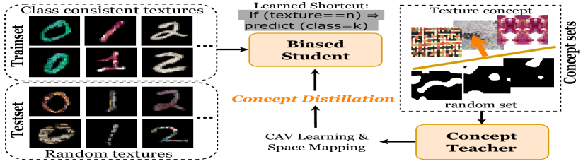
Figure 1: Overview of our approach: The generic conceptual knowledge of a capable teacher can be distilled to a student for performance improvement through bias removal and prior induction.

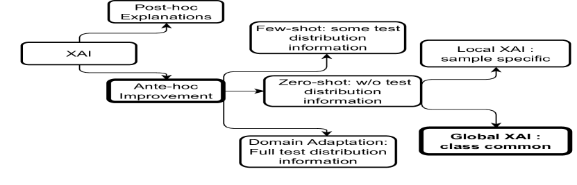
Figure 2: Categorization of related works with ours highlighted.

We also extend concepts to work effectively on intermediate layers of the model, where the sensitivity is more pronounced. Kim et al. [33] measure the final layer’s sensitivity to any intermediate layer outputs. They ask the question: if any changes in activations are done in the intermediate layer, what is its effect on the final layer prediction? They used the final layer’s loss/logit to estimate the model sensitivity, as their interest was to study concept sensitivities for interpretable model prediction. We, on the other hand, aim to fine-tune a model by (de)sensitizing it towards a given concept that may be strongest in another layer [3]. Thus, it is crucial for us to measure the sensitivity in any layer by evaluating the effect of the changes in activations in one intermediate layer on another. We employ prototypes or average class representations in that layer for this purpose. Prototypes are estimated by clustering the class sample activations [12, 80, 44, 52, 51, 68, 46]. Our method, thus, allows intervention in any layer.

In this paper, we present a simple but powerful framework for model improvement using concept loss and concept distillation for a user-given concept defined in any layer of the network. We leverage ideas from post-hoc global explanation techniques and use them in an ante-hoc setting by encoding concepts as CAVs via a teacher model. Our method also admits sample-specific explanations via a local loss [56] along with the global concepts whenever possible. We improve state-of-the-art on classification problems like ColorMNIST and DecoyMNIST [55, 17, 56, 5], resulting in improved accuracies and generalization. We introduce and benchmark on a new and more challenging TextureMNIST dataset with texture bias associated with digits. We demonstrate concept distillation on two applications: (i) debiasing extreme biases on classification problems involving synthetic MNIST datasets [45, 17] and complex and sensitive age-vs.-gender bias in the real-world gender classification on BFFHQ dataset [35] and (ii) prior induction by infusing domain knowledge in the reconstruction problem of Intrinsic Image Decomposition (IID) [40] by measuring and improving disentanglement of albedo and shading concepts. To summarize, we:

• Extend CAVs from post-hoc explanations to ante-hoc model improvement method to sensitize/desensitize models on specific concepts without changing the base architecture.

• Extend the model CAV sensitivity calculation from only the final layer to any layer and enhance it by making it more global using prototypes.

• Introduce concept distillation to exploit the inherent knowledge of large pretrained models as a teacher in concept definition.

• Benchmark results on standard biased MNIST datasets and on a challenging TextureMNIST dataset that we introduce.

• Show application on a severely biased classification problem involving age bias.

• Show application beyond classification to the challenging multi-branch Intrinsic Image Decomposition problem by inducing human-centered concepts as priors. To the best of our knowledge, this is the first foray of concept-based techniques into non-classification problems.

2 Related Work

The related literature is categorized in Fig. 2. Post-hoc (after training) explainability methods include Activation Maps Visualization [64], Saliency Estimation [58], Model Simplification [77], Model Perturbation [18], Adversarial Exemplar Analysis [23], etc. See recent surveys for a comprehensive discussion [82, 16, 48, 72, 2]. Different concept-based interpretability methods are surveyed by Hitzler and Sarker [28], Schwalbe [63], Holmberg et al. [29].

The ante-hoc model improvement techniques can be divided into zero-shot [78], few-shot [74], and multi-shot (domain-adaptation [73]) categories based on the amount of test distribution needed. In zero-shot training, the model never sees the distribution of test samples [78], while in few-shot, the model has access to some examples from the distribution of the test set [74]. Our method works with abstract concept sets (different than any test sample), being essentially a zero-shot method but can take advantage of few-shot examples, if available, as shown in results on BFFHQ subsection 4.1. We restrict the discussion to the most relevant model improvement methods.

Ross et al. [56] penalize a model if it does not prefer the Right answers for Right Reasons (RRR) by using explanations as constraints. EG Erion et al. [17] augment gradients with a penalizing term to match with user-provided binary annotations. More details are available in relevant surveys [19, 76, 25, 8].

Based on the scope of explanation, the existing XAI methods can be divided into global and local methods [82]. Global methods [33, 21] provide explanations that are true for all samples of a class (e.g. ‘stripiness’ concept is focused for the zebra class or ‘red color’ is focused on the prediction of zero) while local methods [1, 64, 65, 57] explain each of samples individually often indicating regions or patches in the image which lead the model to prediction (example, this particular patch (red) in this image was focused the most for prediction of zero). Kim et al. [33] quantify concept sensitivity using CAVs followed by subsequent works [67, 81, 62]. Kim et al. [33] sample sensitivity is local (sample specific) while they aggregate class samples for class sample sensitivity estimation, which makes their method global (across classes). We enhance their local sample sensitivity to the global level via using prototypes that capture class-wide characteristics by definition [12].

Only a few concept-oriented deep learning methods train neural networks with the help of concepts [60, 59]. Concept Bottleneck Models (CBMs) [37], Concept-based Model Extraction (CME) [31], and Self-Explaining Neural Networks (SENNs) [4] predict concepts from inputs and use them to infer the output. CBMs [37] require concept supervision, but CME [31] can train in a partially supervised manner to extract concepts combining multiple layers. SENN [4] learns interpretable basis concepts by approximating a model with a linear classifier. These methods require architectural modifications of the base model to predict concepts. Their primary goal is interpretability, which differs from our model improvement goal using specific concepts without architectural changes. Closest to our work is ClArC [5], which leverages CAVs to manipulate model activations using a linear transformation to remove artifacts from the final results. Unlike them, our method trains the DNN to be sensitive to any specific concept, focusing on improving generalizability for multiple applications.

DFA [43] and EnD [69] use bias-conflicting or out-of-distribution (OOD) samples for debiasing using few-shot generic debiasing. DFA uses a small set of adversarial samples and separate encoders for learning disentangled features for intrinsic and biased attributes. EnD uses a regularization strategy to prevent the learning of unwanted biases by inserting an information bottleneck using pre-known bias types. It is to be noted that both DFA and EnD are neither zero-shot nor interpretability-based methods. In comparison, our method works in both known bias settings using abstract user-provided concept sets and unknown bias settings using the bias-conflicting samples. Our Concept Distillation method is a concept sensitive training method for induction of concepts into the model, with debiasing being an application. Intrinsic Image Decomposition (IID) [11, 20] involves decomposing an image into its constituent Reflectance ($R$) and Shading ($S$) components [40, 49] which are supposed to be disentangled [49, 24].

We use CAVs for inducing R and S priors in a pre-trained SOTA IID framework [47] with improved performance. To the best of our knowledge, we are the first to introduce prototypes for CAV sensitivity enhancement. However, prototypes have been used in the interpretability literature before to capture class-level characteristics [34, 79, 32] and also have been used as pseudo-class labels before [12, 80, 44, 52, 51, 68, 46]. Some recent approaches [30, 66] use generative models to generate bias-conflicting samples (e.g. other colored zeros in ColorMNIST) and train the model on them to remove bias. Specifically, Jain et al. [30] use SVMs to find directions of bias in a shared image and language space of CLIP [54] and use Dall-E on discovered keywords of bias to generate bias-conflicting samples and train the model on them. Song et al. [66] use StyleGAN to generate bias-conflicting samples. Training on bias-conflicting samples might not always be feasible due to higher annotation and computation costs.

One significant difference between such methods [30, 66] is that they propose data augmentation as a debiasing strategy, whereas we directly manipulate the gradient vectors, which is more interpretable. Moayeri et al. [50] map the activation spaces of two models using the CLIP latent space similarity. Due to the generality of the CLIP latent space, this approach is helpful to encode certain concepts like ’cat, dog, man,’ but it is not clear how it will work on abstract concepts with ambiguous definitions like ’shading’ and ’reflectance’ as seen in the IID problem described above.

Figure 3: $v^{l}_{c}$ is calculated as normal to the separating hyperplane of concept set activations (textures $C$ vs. random set $C^{\prime}$ here). A model biased towards $C$ will have its class samples’s loss gradient $\nabla L_{p}$ along $v^{l}_{c}$ (measured by sensitivity $S_{C,k,l}(x)$). To desensitize the model for $C$, we perturb $\nabla L_{p}$ to be parallel to the decision boundary by minimizing the cosine of the projection angle.

Figure 4: Datasets used: ColorMNIST (top row), TextureMNIST (next row), DecoyMNIST (third row), and BFFHQ (bottom rows). Concepts used include color, textured and gray patches, and bias-conflicting samples shown on the right.

3 Concept Guidance and Concept Distillation

Concepts have been used to explain model behavior in a post-hoc manner in the past. Response to abstract concepts can also demonstrate the model’s intrinsic preferences, biases, etc. Can we use concepts to guide the behavior of a trained base model in desirable ways in an ante-hoc manner? We describe a method to add a concept loss to achieve this. We also present concept distillation as a way to take advantage of large foundational models with more exposure to a wide variety of images.

3.1 Concept Sensitivity to Concept Loss

Building on Kim et al. [33], we represent a concept $C$ using a Concept Activation Vector (CAV) as the normal ${v_{C}^{l}}$ to a linear decision boundary between concept samples $C$ from others $C^{\prime}$ in a layer $l$ of the model’s activation space (Fig. 4). The model’s sensitivity $S_{C,l}(\boldsymbol{x})=\nabla L_{o}\left(f_{l}(\boldsymbol{x})\right)\cdot{v}_{C}^{l}$ to $C$ is the directional derivative of final layer loss $L_{o}$ for samples $\boldsymbol{x}$ along ${v_{C}^{l}}$ [33]. The sensitivity score quantifies the concept’s influence on the model’s prediction. A high sensitivity for color concepts may indicate a color bias in the model.

These scores were used for post-hoc analysis before ([33]). We use them ante-hoc to desensitize or sensitize the base model to concepts by perturbing it away from or towards the CAV direction (Fig. 4). The gradient of loss indicates the direction of maximum change. Nudging the gradients away from the CAV direction encourages the model to be less sensitive to the concept and vice versa. For this, we define a concept loss $L_{C}$ as the absolute cosine of the angle between the loss gradient and the CAV direction

$$\small L_{C}(\boldsymbol{x})=|\cos(\nabla L_{o}\left(f_{l}(\boldsymbol{x})\right),\boldsymbol{v}_{C}^{l})|,$$ (1)

which is minimized when the CAV lies on the classifier hyperplane (Fig. 4). We use the absolute value to avoid introducing the opposite bias by pushing the loss gradient in the opposite direction. A loss of $(1-L_{C}(x))$ will sensitize the model to $C$. We fine-tune the trained base model for a few epochs using a total loss of $L=L_{o}+\lambda L_{C}$ to desensitize it to concept $C$, where $L_{o}$ is the base model loss.

3.2 Concepts using Prototypes

Concepts can be present in any layer $l$, though the above discussion focuses on the sensitivity calculation of the final layer using model loss $L_{o}$. The final convolutional layer is proven to learn concepts better than other layers [3]. We can estimate the concept sensitivity of any layer using a loss for that layer. How do we get a loss for an intermediate layer, as no ground truth is available for it?

Class prototypes have been used as pseudo-labels in intermediate layers before [12, 80, 44]. We adapt prototypes to define a loss in intermediate layers. Let $f_{l}(x)$ be the activation of layer $l$ for sample $x$. We group the $f_{l}(x)$ values of the samples from each class into K clusters. The cluster centers $P_{i}$ together form the prototype for that class. We then define prototype loss for each training sample $x$ using the prototype corresponding to its class as

$$L_{p}(x)=\frac{1}{K}\sum_{k=1}^{K}\left\lVert f_{l}(x)-P_{k}\right\rVert^{2}.$$ (2)

We use $L_{p}$ in place of $L_{o}$ in Eq. 1 to define the concept loss in layer $l$. The prototype loss facilitates the use of intermediate layers for concept (de)sensitization. Experiments reported in Tab. 3 confirm the effectiveness of $L_{p}$. Prototypes also capture sample sensitivity at a global level using all samples of a class beyond the sample-specific levels. We update the prototypes after a few iterations as the activation space evolves. If $P^{n}$ is the prototype at Step $n$ and $P^{c}$ the cluster centres using the current $f_{l}(x)$ values, the next prototype is $P_{k}^{n+1}=(1-\alpha)P_{k}^{n}+\alpha P^{c}_{k}$ for each cluster $k$.

3.3 Concept Distillation using a teacher

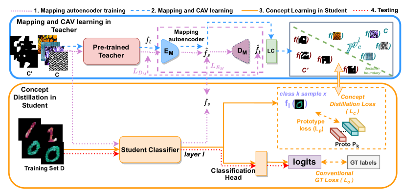
Figure 5: Our framework comprises a concept teacher and a student classifier and has the following four steps: 1) Mapping teacher space to student space for concepts $C$ and $C^{\prime}$ by training an autoencoder $E_{M}$ and $D_{M}$ (dotted purple lines); 2) CAV ($\boldsymbol{v^{l}_{c}}$) learning in mapped teacher space via a linear classifier LC (dashed blue lines); 3) Training the student model with Concept Distillation (solid orange lines): We use $\boldsymbol{v^{l}_{c}}$ and class prototypes loss $L_{p}$ to define our concept distillation loss $L_{c}$ and use it with the original training loss $L_{o}$ to (de)sensitize the model for concept $C$; 4) Testing where the trained model is applied (dotted red lines)

Algorithm 1 Concept Distillation Pipeline

Given: A pretrained student model which is to be fine-tuned for concept (de)sensitization and a pretrained teacher model which will be used for concept distillation. Known Concepts $C$ and negative counterparts (or random samples) $C^{\prime}$, student training dataset $\mathcal{D}$, and student bottleneck layer $l$, #iterations to recalculate CAVs cav_update_frequency, #iterations to update prototypes proto_update_frequency.

1:Concept Distillation:

2: For all class samples in $\mathcal{D}$, estimate class prototypes $P_{k\in\{0,K\}}^{0}$ with K-means.

3: Current iteration $n=0$, initial prototypes $P^{0}=P^{c}$.

4: While not converge do:

5:  If n = 0 or (update_cavs and n % cav_update_frequency = 0) then:

6:   Learn Mapping module:

7:    Forward pass $x\in C\cup C^{\prime}$ from Teacher and Student to get their concept activations $f_{t}$ and $f_{s}$.

8:    Learn the mapping module as autoencoders $E_{M}$ and $D_{M}$.

9:   CAV learning in mapped teacher’s space:

10:    $\mathbf{v}_{C}^{l}$ learned by binary linear classifier as normal to decision boundary of $E_{M}(f_{t}(x))$ for $x\in C$ vs $E_{M}(f_{t}(x^{\prime}))$ for $x^{\prime}\in C^{\prime}$.

11:  If $n$ % proto_update_frequency $=0$ and $n\neq 0$ then:

12:   Estimate new class prototypes $P^{c}_{k\in\{0,K\}}$ with K-means.

13:   Weighted Proto-type $P_{k}^{n+1}=(1-\alpha)P_{k}^{n}+\alpha P^{c}_{k}$.

14:  Else:

15:   $P_{k}^{n+1}=P_{k}^{n}$

16:  Train student with loss $L_{C}+L_{o}$.

17:  $n+=1$.

Concepts are learned from the base model in the above formulation. Base models may have wrong concept associations due to their training bias or limited exposure to concepts. We verify this by an experiment on CAV learning comparison shown in subsection 4.1.

Can we alleviate this problem using a larger model that has seen vast amounts of data as a teacher in a distillation framework?

We use the DINO [13], a self-supervised model trained on a large number of images, as the teacher and the base model as the student for concept distillation. The teacher and student models typically have different activation spaces. We map the teacher space to the student space before concept learning. The mapping uses an autoencoder [27] consisting of an encoder $E_{M}$ and a decoder $D_{M}$ (Fig. 5). As a first step, the autoencoder (Fig. 5) is trained to minimize the loss $L_{D_{M}}+L_{E_{M}}$. $L_{D_{M}}$ is the pixel-wise L2 loss between the original ($f_{t}$) and decoded ($\hat{f}_{t}$) teacher activations and $L_{E_{M}}$ is the pixel-wise L2 loss between the mapped teacher ($\hat{f}_{s}$) and the student ($f_{s}$) activations. The mapping is learned over the concept set of images $C$ and $C^{\prime}$. See the dashed purple lines in Fig. 5.

Next, we learn the CAVs in the distilled teacher space $\hat{f}_{s}$, keeping the teacher, student, and mapping modules fixed. This is computationally light as only a few (50-150) concept set images are involved. The learned CAV is used in concept loss given in Eq. 1. Please note that $E_{M}$ is used only to align the two spaces and can be a small capacity encoder, even a single layer trained in a few epochs.

Taking only Robust learned CAVs for Distillation:

[33] use t-testing with concept vs. multiple random samples to filter robust CAVs for TCAV score estimation. Similar to them, we employed t-testing initially by taking concept vs multiple random samples and selecting only the significant CAVs. This proved to be too expensive computationally during training, especially during frequent CAV updates. Currently, we have a simple filter on CAV classification accuracy > 0.7 to select only the good CAVs (i.e., CAVs that can differentiate concept vs random). The concept loss corresponding to all such valid CAVs is then averaged before backpropagating. This design simplification was empirically verified and found to work equivalently to [33] t-testing).

Choosing the Student Layer for Concept Distillation:

CAVs can be calculated for any model layer. Which student layers should be used? We show results only for the last convolution layer of the student model in the paper, but theoretically, our framework can be extended to any number of layers at any depth. Our design choice is based on the fact that the deeper layers of the model encode complex higher-order class-level features while the shallower layers encode low-level features. The last convolution layer represents more abstract features, which are easily representable for humans in the form of concepts rather than low-level features in other layers. For the same reasons, [3] too use the last convolution layers for conceptual explanation generation.

4 Experiments

We demonstrate the impact of the concept distillation method on the debiasing of classification problems as well as improving the results of a real-world reconstruction problem. Classification experiments cover two categories of Fig. 2: the zero-shot scenario, where no unbiased data is seen, and the few-shot scenario, which sees a few unbiased data samples. We use pre-trained DINO ViT-B8 transformer [13] (more details on teacher selection in Appendix C) as the teacher. We use the last convolution layer of the student model for concept distillation. The mapping module ($<120K$ parameters, $<10$MB), CAV estimations (logistic regression, $<1$MB), and prototype calculations all complete within a few iterations of training, taking 15-30 secs on a single 12GB Nvidia 1080 Ti GPU. Our framework is computationally light. In our experimentation reported below, we fix the CAVs as initial CAVs and observe similar results as varying them. Uur concept sensitive fine-tuning method converges quickly, and hence updating CAVs in every few iterations does not help (Appendix B). Where relevant, we report average accuracy over five training runs with random seeds ($\pm$ indicates variance).

4.1 Concept Sensitive Debiasings

We show results on two standard biased datasets (ColorMNIST [45] and DecoyMNIST [17]) and introduce a more challenging TextureMNIST dataset for quantitative evaluations. We also experimented on a real-world gender classification dataset BFFHQ [35] that is biased based on age. We compare with other state-of-the-art interpretable model improvement methods [55, 56, 17, 69, 43, 5]. Fig. 4 summarizes the datasets, their biases, and the concept sets used.

Poisoned MNIST Datasets: ColorMNIST [45] has MNIST digit classes mapped to a particular color in the training set [55]. The colors are reversed in the test set. The baseline CNN model (Base) trained on ColorMNIST gets 0% accuracy on the 100% poisoned test set, indicating that the model learned color shortcuts instead of digit shapes. We esitmate the CAV for color concept using color patches vs. random shapes (negative concept) and use our concept loss to debias the model (Fig. 4). We now discuss an example which shows why CAV learning in same model is not ideal.

CAV Learning comparison:

In ColorMNIST, class zeros are always associated with the color red. We learn a CAV for the concept of red ($CAV_{red}$ separating red patches with other colored patches) in each teacher, mapped teacher and base model (biased initial Student) and measure its cosine similarity (cs) with the respective model representations for concept images of red, red-zeros.

As seen from Tab. 1, the Teacher and Mapped Teacher have cs(red) > cs(red_zeros) < cs(red_non_zeros) which indicate correct concept learning while the Student (Base Model) has cs(red) < cs(red_zeros) < cs(red_non-zeros) that indicates confusion of bias with concept (concept red-zeros confused with concept red). Thus, teacher’s CAV and its mapped version capture the intended concept well, while the base model (student) confuses the red-zeros concept with CAV. This small demonstration shows (a) why the teacher is needed for good CAV learning and (b) how well CAV’s are transferred to the student via the mapping module. Mapping module does not bias the CAV representation.

Table 1: Cosine Similarity Order of concepts with $CAV_{red}$

Model	’red’	’red_zeros’	’red_non_zeros’	’non_red_zeros’
Teacher	0.084	-0.013	-0.009	0.005
Mapped Teacher	0.287	-0.044	0.014	0.024
Base Model	-0.023	-0.019	-0.013	0.000

Results:

We show results comparison on the usage of teacher and prototypes component of our method in Tab. 3. As can be seen from Tab. 3, our method of using intermediate layer sensitivity via prototypes as described in subsection 3.2 yields better results. Similarly, usage of teacher (described in subsection 3.3) facilitates better student concept learning as shown above. Our concept sensitive training not only improves student accuracy but observes evident reduction in TCAV scores [33] of bias concept as seen from Tab. 3.

Tab. 4 compares our results with the best zero-shot interpretability based methods, i.e., CDEP [55], RRR [56], and EG [17]. Our method improves the accuracy from 31% by CDEP to 41.83%, and further to 50.93% additionally with the local explanation loss from [56] (loss details in Appendix A).

Table 2: Main components of our method shown on ColorMNIST dataset: Ours usage of teacher and proto-types yields the best performance.

Teacher?	Prototype?	Accuracy
✗	✗	9.96
✗	✓	26.97
✓	✗	30.94
✓	✓	50.93

Table 3: TCAV scores of bias concept: Our concept sensitive training significantly decreases the sensitivity of model towards bias.

Dataset	Concept	Base Model	Ours
ColorMNIST	Color	0.52	0.21
DecoyMNIST	Spatial patches	0.57	0.45
TextureMNIST	Textures	0.68	0.43
BFFHQ	Age	0.78	0.13

Table 4: Comparison of the accuracy of our method with other zero-shot interpretable model-improvement methods. All methods require user-level intervention: Our method requires concept sets, while others (CDEP, RRR, EG) require user-provided rules.

Dataset	Bias	Base	CDEP[55]	RRR[56]	EG[17]	Ours w/o Teacher	Ours	Ours+L
ColorMNIST	Digit color	0.1	31.0	0.1	10.0	26.97	41.83	$\boldsymbol{50.93_{\pm 1.42}}$
DecoyMNIST	Spatial patches	52.84	97.2	99.0	97.8	87.49	98.58	$\boldsymbol{98.98_{\pm 0.20}}$
TextureMNIST	Digit textures	11.23	10.18	11.35	10.43	38.72	48.82	$\boldsymbol{56.57_{\pm 0.79}}$

Figure 6: Left: Comparison of our method and ClArC [5] on 20% biased ColorMNIST. Right: GradCAM [64] visualizations (more red, more important) on (i) TextureMNIST (middle image) (ii) Extreme case when the color bias is in the background (bottom) instead of foreground (top). Our model focuses on the shape more than CDEP (which is more blue in the foreground).

GradCAM [64] visualizations in Fig. 6 show that our trained model focuses on highly relevant regions. Fig. 6 left compares our class-wise accuracy on 20% biased ColorMNIST with ClArC [5], a few-shot global method that uses CAVs for artifact removal. (ClArC results are directly reported from their main paper due to the unavailability of the public codebase.) ClArC learns separate CAVs for each class by separating the biased color digit images (e.g. red zeros) from the unbiased images (e.g. zeros in all colors). A feature space linear transformation is then applied to move input sample activations away/towards the learned CAV direction. Their class-specific CAVs definition can not be generalized to test sets with multiple classes. This results in a higher test accuracy variance as seen in Fig. 6. Further, as they learn CAVs in the biased model’s activation space, a common concept set cannot be used across classes.

DecoyMNIST [17] has class indicative gray patches on image boundary that biased models learn instead of the shape. We define concept sets as gray patches vs. random set (Fig. 4) and report them in Tab. 4 second row. All methods perform comparably on this task as the introduced bias does not directly corrupt the class intrinsic attributes (shape or color), making it easy to debias. TextureMNIST is a more challenging dataset that we have created for further research in the area. Being an amalgam of colors and patterns, textures are more challenging as a biasing attribute. Our method improves the performance while others struggle on this task (Tab. 4 last row). Fig. 6 shows that our method can focus on the right aspects for this task.

Table 5: Our method improves the model using human-centered concepts and shows better generalization to different datasets, while CDEP, which uses pixel-wise color rules, cannot.

	ColorMNIST Trained			TextureMNIST Trained
Test Dataset	Base	CDEP[55]	Ours+L	Base	CDEP[55]	Ours+L
Invert color	0.00	23.38	50.93	11.35	10.18	45.36
Random color	16.63	37.40	46.62	11.35	10.18	64.96
Random texture	15.76	28.66	32.30	11.35	10.18	56.57
Pixel-hard	15.87	33.11	38.88	11.35	10.18	61.29

Generalization to multiple biasing situations is another important aspect. ColorMNIST and TextureMNIST datasets have test sets comprising flipped colors and random textures digits. To check the generalization of our model, we test the ColorMNIST and TextureMNIST trained models by creating different test sets having random colors and textures. Inverted color is the original test set of ColorMNIST wherein the associated digits colors are reversed. e.g. red color is changed to 1-red for digit 0, orange is changed to 1-orange for digit 1 and so on. We create Random color test dataset where the digit colors are randomised (e.g. red zeros changed to random color zeros). We used randomised textures as original test set of TextureMNIST. All of the above datasets including ColorMNIST and TextureMNIST have only one particular color/texture in entire digit. We randomise each pixel color by creating a Pixel-hard test set (Fig. 7).

Figure 7: pixel hard MNIST test set

Tab. 5 shows the performance on different types of biases by differently debiased models. Our method performs better than CDEP in all situations. Interestingly, our texture-debiased model performs better on color biases than CDEP debiased on the color bias! We believe this is because textures inherently contain color information, which our method can leverage efficiently. Our method effectively addresses an extreme case of color bias introduced in the background of ColorMNIST, a dataset originally biased in foreground color. By introducing the same color bias to the background and evaluating our ColorMNIST debiased models, we test the capability of our approach. In an ideal scenario where color debiasing is accurate, the model should prioritize shape over color, a result achieved by our method but not by CDEP as shown in Fig. 6.

Table 6: Comparisons in few-shot setting: Our method is not limited to user-provided concept sets and can also work with bias-conflicting samples. We compare our accuracy over the BFFHQ dataset [35] with other few-shot debiasing methods.

Dataset	Bias	Base	EnD [69]	DFA [43]	Ours w/o Teacher	Ours
BFFHQ	Age	$56.87_{\pm 2.69}$	$56.87_{\pm 1.42}$	$61.27_{\pm 3.26}$	59.4	$\bf 63_{\pm 0.79}$

BFFHQ [35] dataset is used for the gender classification problem. It consists of images of young women and old men. The model learns entangled age attributes along with gender and gets wrong predictions on the reversed test set i.e. old women and young men. We use the bias conflicting samples by Lee et al. [43] – specifically, old women vs. women and young men vs. men – as class-specific concept sets.We compare against recent debiasing methods EnD [69] and DFA [43]. Tab. 6 shows our method getting a comparable accuracy of 63%. We also tried other concept set combinations: (i) old vs. young (where both young and old concepts should not affect) $\xrightarrow{}$ 62.8% accuracy, (ii) old vs. mix (men and women of all ages) and young vs. mix $\xrightarrow{}$ 62.8% accuracy, (iii) old vs. random set (consisting of random internet images from [33]) and young vs. random $\xrightarrow{}$ 63% accuracy. These experiments indicate the stability of our method to the concept set definitions. This proves our method can also work with bias-conflicting samples [43] and does not necessarily require concept sets (Tab. 6). We also experimented by training class-wise (for all women removing young bias followed by men removing old bias and vice versa) vs training for all classes together (both men, women removing age bias as described above) and observed similar results, suggesting that our concept sensitive training is robust to class-wise or all class agnostic training. Local interpretable improvement methods like CDEP, RRR, and EG are not reported here as they cannot capture complex concepts like age due to their pixel-wise loss or rule-based nature.

Table 7: Increasing the bias of the teacher on ColorMNIST reduces accuracy.

Teacher’s Training Data Bias%	No Distil	5	10	25	75	90	100
Student Accuracy%	26.97	40.47	33.18	30.38	28.74	23.23	23.63

Discussion

No Distillation Case: We additionally show our method without teacher (Our Concept loss with CAVs learned directly in student) in all experiments as "Ours w/o Teacher" and find inferior performance when compared to Our method with Distillation.

Case of Ideal Teacher Student Mapping: In theory, if the mapping module has a zero-loss, it could make the distillation case the same as the case without distillation, but this is not observed in our experiments due to two main reasons: (i) We use the mapping module to map only the conceptual knowledge in CAV and train it only for concept sets and not the training samples. (ii) Due to major differences in the perceived notion of concepts in teacher and student networks and due to a simple mapping autoencoder (one upconv and downconv layer) the MSE loss never goes to zero (e.g, in ColorMNIST, it starts from  11 and converges at  5 for DINO teacher to biased student alignment). In our initial experiments, we tried bigger architectures (ResNet18+) and found improved mapping losses but decreased student performances. Mapping Encoder encodes an expert’s knowledge into the system via the provided concept sets, quantifies this knowledge as CAV via a generalized teacher model trained on large amount of data, and thus helps in inducing it via distillation into the student model. This brings threefold advantages in our system: expert’s intuition, large model’s generality, and efficiency of distillation.

Bias in Teacher: We check the effect of bias in teacher by training it with varying fractions of OOD samples to bias them. Specifically, we use the same student architecture for the teacher. The teacher is trained on the ColorMNIST dataset with 5, 10, 25, 50, 75, and 90% biased color samples in the trainset (e.g. $k\%$ bias indicates $k\%$ red zeros). The resulting concept-distilled system is then tested on the standard 100% reverse color setting of ColorMNIST. Tab. 7 shows that concept distillation improves performance even with high teacher bias, though accuracy decreases with the increasing bias in teacher. Apparently, 100% bias in teacher in this setting of teacher with same architecture as the student is essentially CAV learning in same model case (No Distil). Here, the improvements are due to prototypes, and as can be seen, there is a slight degradation in performance of 100% bias vs No Distil (23.63 vs 26.97). This can be attributed to an error due to the mapping module. Apart from biased small teacher experiments in Tab. 6 where we vary the bias in teacher from 5% to 100%, we also experimented when the small teacher network is (pre)trained on 0% bias (simply MNIST dataset [42]). We found the student to achieve an accuracy of 23.6% with this teacher network. This accuracy is lesser than that in biased teacher due to the fact that the teacher trained on the MNIST dataset having grayscale images has never seen the concept of color. Henceforth as mentioned before, it is important for teacher to have the knowledge of concepts for concept distillation to work well.

Ablations

Table 8: Impact of different variants of CAV sensitivity calculation gradient $\nabla X$ in proposed loss Eq. 1 on the final results

X	logit	$L_{o}$	$L_{p},\text{fixed proto}$	$L_{p},\text{varying prototypes}$ (Ours)
Accuracy %	25.55	30.94	40.02	41.83

We experimented with different ways of calculating sensitivity used for $L_{c}$ in Eq. 1 by replacing $\nabla L_{o}$ with $\nabla X$ where $X$ is taken as (i) last layer outputs or logits; (ii) last layer loss $L_{o}$ and (iii) intermediate layer prototype based loss $L_{p}$ in two settings: fixed prototypes where prototypes are kept fixed as initial ($\alpha=0$) vs prototypes are varied with $\alpha$. Settings (i) and (ii) are essentially final layer sensitivity calculation according to the original implementation by Kim et al. [33] while Setting (iii) is our proposed intermediate layer sensitivity using prototypes. We also show results when (a) KNN k in the prototype calculation is varied and found k=7 to work best Fig. 8 (b) number of images (#imgs) in the concept set are varied and we observe a peak in #imgs = 150 which is chosen as the KNN k and #imgs in our experiments.

Figure 8: Impact of varying the concept set size and number of means on 100% biased ColorMNIST.

4.2 Prior Knowledge Induction

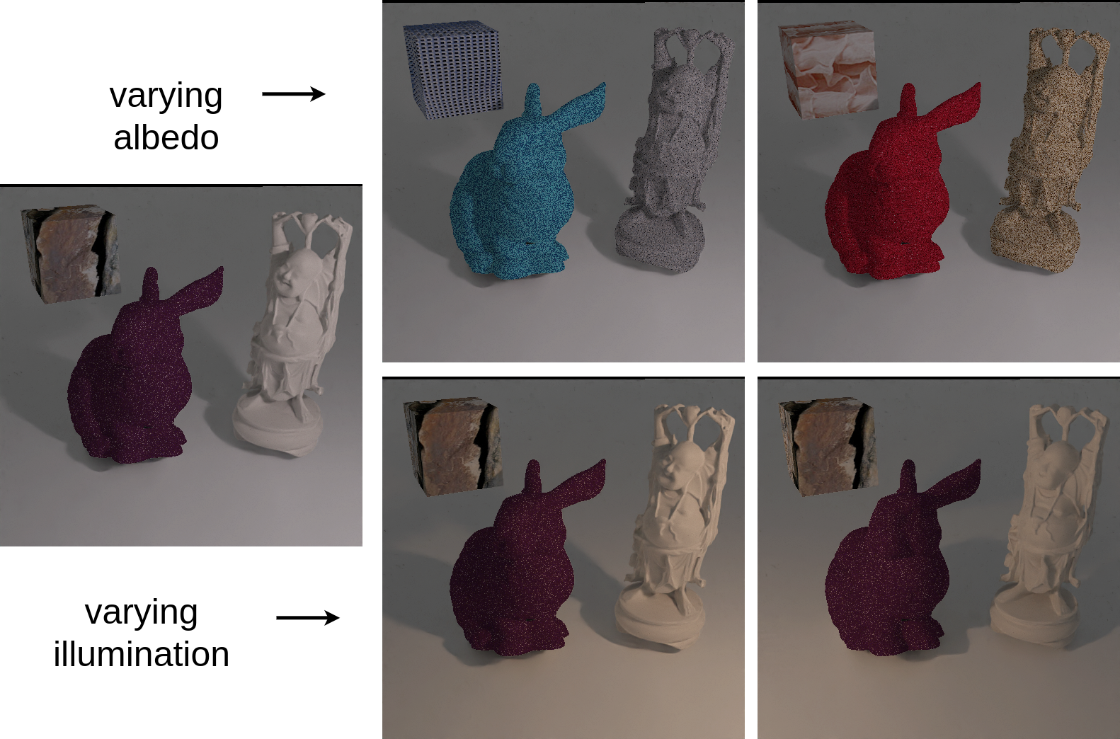
Figure 9: Concept sets used for IID experiments

Table 9: IID performance on ARAP dataset: Inducing human-centered concepts like albedo-invariance of S and illumination invariance of R results in improved IID performance.

Model	MSE R $\downarrow$	MSE S $\downarrow$	SSIM R $\uparrow$	SSIM S $\uparrow$	Synthetic		Real-World
					CSM R $\uparrow$	CSM S $\uparrow$	CSM R $\uparrow$
CGIID [47]	0.066	0.027	0.536	0.581	1.790	0.930	5.431
CGIID++	0.080	0.032	0.520	0.552	0.860	0.401	3.421
Ours (R only)	0.052	0.027	0.54	0.581	1.889	1.260	4.89
Ours (R & S)	0.059	0.028	0.538	0.586	6.040	1.023	78.46

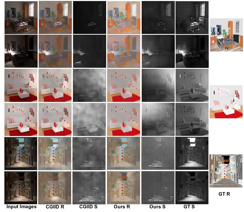
Figure 10: Qualitative IID results: Our method uses complex concepts like albedo and illumination to enhance $\hat{R}$ and $\hat{S}$ predictions that are illumination and albedo invariant respectively. First column shows two input images of the same scene under varying illumination. Next two columns are Reflectance and Shading results from baseline method, followed by ours. Last two columns show the two ground truth shading components and the common reflectance image. Our method is able to make the $\hat{R}$ less sensitive to illumination (thereby removing the concept of illumination from $\hat{R}$ and during this $\hat{R}$ predictions become flatter without specifically introducing the flatness prior suggesting disentanglement of R-S is a better way to improve IID. Also, the illumination information removed from $\hat{R}$ is introduced in $\hat{S}$.

Intrinsic Image Decomposition (IID) is an inverse rendering problem [7] based on the retinex theory [41], which suggests that an image $I$ can be divided into Reflectance $R$ and Shading $S$ components such that $I=R\cdot S$ at each pixel. Here $R$ represents the material color or albedo, and $S$ represents the scene illumination at a point. As per definition, $R$ and $S$ are disentangled, with $R$ invariant to illumination and $S$ invariant to albedo. As good ground truth for IID is hard to create, IID algorithms are evaluated on synthetic data or using some sparse manual annotations [9, 38]. Gupta et al. [24] use CAV-based sensitivity scores to measure the disentanglement of $R$ and $S$. They create concept sets of (i) varying albedo: wherein the albedo (material color) of the scene is varied(ii) varying illumination: where illumination is varied (Fig. 9).

From the definition of IID, Reflectance shall only be affected by albedo variations and not by illumination variations and vice-versa for Shading. They defined Concept Sensitivity Metric (CSM) to measure $R$-$S$ disentanglement and evaluate IID methods post-hoc. Using our concept distillation framework, we extend their post-hoc quality evaluation method to ante-hoc training of the IID network to increase disentanglement between $R$ and $S$. We train in different experimental settings wherein we only train the $R$ branch ($R$ only) and both $R$ and $S$ branches together ($R\&S$) with our concept loss in addition to the original loss [47] and report results in Tab. 9.

We choose the state-of-the-art CGIID [47] network as the baseline. The last layer of both $R$ and $S$ branches is used for concept distillation, and hence no prototypes are used. Following Li and Snavely [47], we fine-tune over the CGIntrinsics [47], IIW [10], and SAW [39] datasets while we report results over ARAP dataset [11], which consists of realistic synthetic images. For $L_{o}$, we adopt the same losses as Li and Snavely [47], which consist of an IIW loss, GT Reconstruction loss, and a SAW loss. For concept sets, we follow [24]. They create the concepts of varying albedo and varying illumination on different objects and scenes keeping the viewpoint fixed. They create scenes consisting of single object and multiple objects and render them in blender. Following them, we use 100 images per scene for varying albedo concept and 44 for varying illumination concept. We train the model for 5-10 epochs, saving the best checkpoint (on validation). Our method converges in 16-20 hours on two 12GB Nvidia 1080 Ti GPUs.

We also train the baseline model for additional epochs to get CGIID++ for a fair comparison. Tab. 9 shows different measures to compare two variations of our method with CGIID and CGIID++ on the ARAP dataset [11]. We see improvements in MSE and SSIM scores which compare dense-pixel wise correspondences CSM scores [24] which evaluate R-S disentanglement. Specifically, $CSM_{S}$ measures albedo invariance of S and $CSM_{R}$ measures illumination invariance of R predictions. We report CSM scores in two concept set settings of Synthetic vs Real-World from Gupta et al. [24]. The improvement in MSE and SSIM scores appear minor quantitatively, but our method performs significantly better in terms of CSM scores. It also observes superior performance qualitatively, as seen in (Fig. 10). Our $R$ outputs are less sensitive to illumination, with most of the illumination effects captured in $S$.

Discussion and Limitations:

Our concept distillation framework can work on different classification and reconstruction problems, as we demonstrated. Our method can work well in both zero-shot (with concept sets) and few-shot (with bias-conflicting samples) scenarios. Bias-conflicting samples may not be easy to obtain for many real-world applications. Our required user-provided concept samples can incur annotation costs, though concept samples are usually easier to obtain than bias-conflicting samples. When neither bias-conflicting samples nor user-provided concept sets are available, concept discovery methods like ACE [22] could be used. ACE discovers concepts used by the model by image super-pixel clustering. Automatic bias detection methods like Bahadori and Heckerman [6] can be used to discover or synthesize bias-conflicting samples for our method. Our method can also be used to induce prior knowledge into complex reconstruction/generation problems, as we demonstrated with IID. The dependence on the teacher for conceptual knowledge could be another drawback of our method, as with all distillation frameworks [26].

Societal Impact: Our method can be used to reduce or increase the bias by the appropriate use of the loss $L_{C}$. Like all debiasing methods, it thus has the potential to be misused to introduce calculated bias into the models.

5 Conclusions

We presented a concept distillation framework that can leverage human-centered explanations and the conceptual knowledge of a pre-trained teacher to distill explanations into a student model. Our method can desensitize ML models to selected concepts by perturbing the activations away from the CAV direction without modifying its underlying architecture. We presented results on multiple classification problems. We also showed how prior knowledge can be induced into the real-world IID problem. In future, we would like to extend our work to exploit automatic bias detection and concept-set definition. Our approach also has potential to be applied to domain generalization and multitask learning problems.

Acknowledgements:

We thank Prof. Vineeth Balasubramanian of IIT Hyderabad for useful insights and discussion. We would also like to thank the four anonymous reviewers of Neurips, 2023 for detailed discussions and comments which helped us improve the paper.

Appendix A Local loss from RRR

To leverage the local explanation benefits apart from the global ones, we additionally use a local loss from RRR [61] for our experiments over ColorMNIST, DecoyMNIST, and TextureMNIST datasets (indicated by $Ours+L$ in Table 1 and Table 2 in paper). RRR [61] has a reasoning loss, which is added to the original GT loss of a classifier with a factor $\lambda$, and is given as:

$$L(\theta,X,y,A)=\underbrace{\sum_{n=1}^{N}\sum_{k=1}^{K}-c_{k}y_{nk}\log\left(\hat{y}_{nk}\right)}_{\text{Right answers }}+\underbrace{\lambda\sum_{n=1}^{N}\sum_{d=1}^{D}\left(A_{nd}\frac{\delta}{\delta h_{nd}}\sum_{k=1}^{K}c_{k}\log\left(\hat{y}_{nk}\right)\right)^{2}}_{\text{Right reasons }}$$

Where $A\in\{0,1\}^{N\times D}$ is the user-provided annotation matrix. It is a binary mask to indicate if dimension $D$ should be irrelevant for the prediction of observation $n$. $\lambda$ is a regularization parameter that ensures that "right answers" and "right reasons" terms have similar orders of magnitude. $N$ is the total number of observations and $\hat{y}_{nk}$ is the predicted probability for class $k$ and observation $n$. RRR penalizes the gradients over the binary mask feature-wise for each input sample and thus is a local XAI method. In the case of debiasing color concept, we take the programmatic rule of single pixel not affecting (single-pixel represents color information) while a group of pixels affecting as demonstrated by [55] for their adaptation of RRR. We additionally experimented by including local interpretability-based losses from CDEP [55], or EG [17] (instead of RRR) for MNIST datasets (ColorMNIST, DecoyMNIST, and TextureMNIST) but found the one in RRR [56] to work best. It is to be noted that local method losses like CDEP [55], RRR [56], or EG [17] require user-given rules. For ColorMNIST and DecoyMNIST, which have the bias of color, they minimize the contribution of individual pixels since the color information is contributed by individual pixels. For the execution of their methods on TextureMNIST, we use the same individual pixel contribution minimization rule. Such rules are not straightforward to extract in case of more complex bias (for example, in BFFHQ), and hence, applying such local XAI-based methods is not feasible.

Appendix B Fixing vs. Varying CAVs in Experiments

Figure 11: Loss Curves in varying cav update iterations: frequent pattern observed, convergence quickly

In our experimentation reported in the above tables in the paper, we fix CAVs. We also experimented with updating CAVs in the student after every few training iterations (50, 100, 200, etc.). Specifically, we experimented in the following settings and report the concept loss $L_{c}$ curves with iterations in Fig. 11.

• cav_update_iter200: CAV updates every 200 iterations.

• cav_update_iter100: CAV updates every 100 iterations.

• constant_cav: Fixed CAV throughout training.

As seen in Fig. 11, there is a recurring pattern with concept loss $L_{C}$ increasing on CAV update (due to an abrupt change in objectives), followed by a subsequent decrease due to optimization. However, $L_{C}$ remains lower than the initial value the model started with (from 105.98 at iteration 0, loss dropped to 9.51 at iteration 199 (before the CAV update) but jumps to 20.61 following the CAV update), underscoring the efficacy of our approach. Similar patterns were consistently observed when updating CAVs in varying numbers of iterations. This trend persisted across diverse datasets during training as well.

The given graph is shown for experimentation over ColorMNIST, but we find the same recurring patterns across all other datasets. Additionally, the best validation accuracy (and also corresponding test accuracy) values for all the settings mentioned above (whether fixed or varying CAVs) are the same (within < 0.3% accuracy changes amongst the settings). The graph also shows that our design choice of keeping CAVs fixed is good practically as the loss quickly converges to a lower value.

Appendix C Design Choices and Implementation Details

Teacher Selection:

For a teacher, we experiment with various model architectures and chose a pre-trained DINO transformer [13] for the main reason of scalability. DINO has been proven to work well for a variety of tasks [70, 75]. A large model knows a variety of concepts and can be used as a teacher for various tasks, as shown in our experiments. We use the same DINO teacher on very different classification datasets like biased MNIST (ColorMNIST, DecoyMNIST, and TextureMNIST) and BFFHQ, as well as over a completely different problem of IID.

Among the DINO variants, we found ViT-B/8 (85M parameters) to perform the best, aiding student to get 50.93% accuracy on ColorMNIST while ViT-S/8 (21M parameters) aced 39% student accuracy. We thus picked DINO ViT-B/8 for all our experiments. We used the code implementation of the DINO feature extractor by Tschernezki et al. [71] and loaded the checkpoints for DINO variants from [13]. The DINO ViT-B/8 gives 768-dimensional feature images, further reduced to 64 using PCA.

Mapping Module:

For the mapping module, we choose a pair of one down-convolutional and up-convolutional layers as Encoder and decoder (depending on students and teacher’s dimensions, it is determined whether the Encoder is up or down-convolutional and vice versa). In our experiments, we train the autoencoder for a maximum of five epochs and select the Encoder from the best of the first five epochs as our activation space mapping module $M$. We also tried with other deeper autoencoder architectures in our initial experiments but found the above simple one to give good results while being computationally cheapest. Due to the simple architecture (logistic regression or single up-down convolutions), both our CAV learning and Mapping module training are very lightweight (< 120K parameters, < 10MB and <1MB) and train within a minute for 10-15 concept sets having a number of images between 50-200 on a single 12GB Nvidia 1080 Ti GPU.

CAV learning:

For CAV learning, we use a logistic regression implemented by a single perceptron layer with sigmoid activation. We train it to distinguish between model activations of concept set (C) and its negative counterpart (C’) in layer $l$ using a cross-entropy loss for binary classification. This is theoretically the same but implementation-wise slightly different from [33], who also use a logistic regression but from sklearn [53]. We get the same results from either of them, though our perceptron-based implementation is slightly faster in terms of computation.

C.1 Debiasing in classification details

For the student network in classification debiasing applications, we use two convolution layers followed by two fully connected layers as done by [55] [43] for all three biased MNIST experiments. We use Resnet18 (no pre-training) for BFFHQ student architecture as done by [43] and apply our method over the "layer4.1.conv1" layer. We use Adam [36] optimizer with a learning rate of 10e-4, $0.9\leq\beta\leq 0.999$, and $ep=1e-08$ with a weight decay of 0 (all default pytorch values except learning late). We use a batch size of 32 for MNIST experiments and 64 for BFFHQ experiments. For the mapping module, we use one up-convolution and one down-convolution layer for encoders and decoders. We train the autoencoders with an L2 loss. For training the MNIST and BFFHQ models, we use the cross-entropy loss as the Ground Truth loss ($L_{o}$). Our concept loss $L_{C}$ is weighted by a parameter $\lambda$ varied from 0.01 to 10e5 in our experiments. We found it to work best for values close to 20 in our experimentation. Other parameter values that we found to work best are number of clusters in K-Means $k=7$ and prototypes updation weight $\alpha=0.3$. Our student model converges within 2-3 epochs of training with a training time of less than 1.5-2 hours for MNIST datasets and within 4 hours for the BFFHQ dataset (on one Nvidia 1080 Ti GPU).

C.1.1 MNIST Details

For MNIST datasets (ColorMNIST and DecoyMNIST), we use the splits by Rieger et al. [55]. For the creation of TextureMNIST, we use the above-obtained splits of digits and replace the colors with textures from DTD [15] (all colors removed and rather texture bias added). We use random flat-colored patches as the concept "color," random textures as the "textures" concept, and gray-colored patches as the "gray" concept set. For the negative concept set, we create randomly shaped white blobs in black backgrounds.

C.1.2 BFFHQ Details

We take the 48 images each for young men and old women (bias conflicting samples as given by Lee et al. [43]) as our concept sets for class-specific training (separate concepts for each class). For the negative concept set of class-specific training, we take mixed images of both young and old women for women concept and young and old men for men concept. We use the same train-test-validation split as done by [43].

References

- Aditya et al. [2018] C. Aditya, S. Anirban, D. Abhishek, and H. Prantik. Grad-cam++: improved visual explanations for deep convolutional networks. arxiv 2018. arXiv preprint arXiv:1710.11063, 2018.
- Akhtar [2023] N. Akhtar. A survey of explainable ai in deep visual modeling: Methods and metrics. ArXiv, abs/2301.13445, 2023.
- Akula et al. [2020] A. Akula, S. Wang, and S.-C. Zhu. Cocox: Generating conceptual and counterfactual explanations via fault-lines. In Proceedings of the AAAI Conference on Artificial Intelligence, volume 34, pages 2594–2601, 2020.
- Alvarez Melis and Jaakkola [2018] D. Alvarez Melis and T. Jaakkola. Towards robust interpretability with self-explaining neural networks. Adv. Neural Inform. Process. Syst., 2018.
- Anders et al. [2022] C. J. Anders, L. Weber, D. Neumann, W. Samek, K.-R. Müller, and S. Lapuschkin. Finding and removing clever hans: Using explanation methods to debug and improve deep models. Information Fusion, 77:261–295, 2022.
- Bahadori and Heckerman [2020] M. T. Bahadori and D. E. Heckerman. Debiasing concept-based explanations with causal analysis. arXiv preprint arXiv:2007.11500, 2020.
- Barrow and Tenenbaum [1978] H. G. Barrow and J. M. Tenenbaum. Recovering intrinsic scene characteristics from images. 1978.
- Beckh et al. [2023] K. Beckh, S. Müller, M. Jakobs, V. Toborek, H. Tan, R. Fischer, P. Welke, S. Houben, and L. von Rueden. Sok: Harnessing prior knowledge for explainable machine learning: An overview. In First IEEE Conference on Secure and Trustworthy Machine Learning, 2023.
- Bell et al. [2014a] S. Bell, K. Bala, and N. Snavely. Intrinsic images in the wild. ACM Transactions on Graphics (TOG), 33:1 – 12, 2014a.
- Bell et al. [2014b] S. Bell, K. Bala, and N. Snavely. Intrinsic images in the wild. ACM Transactions on Graphics (TOG), 33(4):1–12, 2014b.
- Bonneel et al. [2017] N. Bonneel, B. Kovacs, S. Paris, and K. Bala. Intrinsic Decompositions for Image Editing. Computer Graphics Forum (Eurographics State of The Art Report), 2017.
- Caron et al. [2018] M. Caron, P. Bojanowski, A. Joulin, and M. Douze. Deep clustering for unsupervised learning of visual features. In Proceedings of the European conference on computer vision (ECCV), pages 132–149, 2018.
- Caron et al. [2021] M. Caron, H. Touvron, I. Misra, H. Jégou, J. Mairal, P. Bojanowski, and A. Joulin. Emerging properties in self-supervised vision transformers. In Proceedings of the IEEE/CVF international conference on computer vision, pages 9650–9660, 2021.
- Chang [2018] D. T. Chang. Concept-oriented deep learning: Generative concept representations. arXiv preprint arXiv:1811.06622, 2018.
- Cimpoi et al. [2014] M. Cimpoi, S. Maji, I. Kokkinos, S. Mohamed, and A. Vedaldi. Describing textures in the wild. In Proceedings of the IEEE conference on computer vision and pattern recognition, pages 3606–3613, 2014.
- Du et al. [2019] M. Du, N. Liu, and X. Hu. Techniques for interpretable machine learning. Communications of the ACM, 63(1):68–77, 2019.
- Erion et al. [2021] G. Erion, J. D. Janizek, P. Sturmfels, S. M. Lundberg, and S.-I. Lee. Improving performance of deep learning models with axiomatic attribution priors and expected gradients. Nature machine intelligence, 3(7):620–631, 2021.
- Fong and Vedaldi [2017] R. C. Fong and A. Vedaldi. Interpretable explanations of black boxes by meaningful perturbation. In Proceedings of the IEEE international conference on computer vision, pages 3429–3437, 2017.
- Gao et al. [2022] Y. Gao, S. Gu, J. Jiang, S. R. Hong, D. Yu, and L. Zhao. Going beyond xai: A systematic survey for explanation-guided learning. arXiv preprint arXiv:2212.03954, 2022.
- Garces et al. [2022] E. Garces, C. Rodriguez-Pardo, D. Casas, and J. Lopez-Moreno. A survey on intrinsic images: Delving deep into lambert and beyond. Int. J. Comput. Vision, 130(3):836–868, 2022.
- Ghandeharioun et al. [2021] A. Ghandeharioun, B. Kim, C.-L. Li, B. Jou, B. Eoff, and R. W. Picard. Dissect: Disentangled simultaneous explanations via concept traversals. arXiv preprint arXiv:2105.15164, 2021.
- Ghorbani et al. [2019] A. Ghorbani, J. Wexler, J. Zou, and B. Kim. Towards automatic concept-based explanations. arXiv preprint arXiv:1902.03129, 2019.
- Goodfellow et al. [2014] I. J. Goodfellow, J. Shlens, and C. Szegedy. Explaining and harnessing adversarial examples. arXiv preprint arXiv:1412.6572, 2014.
- Gupta et al. [2023] A. Gupta, S. Saini, and P. J. Narayanan. Interpreting intrinsic image decomposition using concept activations. In Proceedings of the Thirteenth Indian Conference on Computer Vision, Graphics and Image Processing, ICVGIP ’22, New York, NY, USA, 2023. Association for Computing Machinery. ISBN 9781450398220. doi: 10.1145/3571600.3571603.
- Hase and Bansal [2021] P. Hase and M. Bansal. When can models learn from explanations? a formal framework for understanding the roles of explanation data. arXiv preprint arXiv:2102.02201, 2021.
- Hinton et al. [2015] G. Hinton, O. Vinyals, and J. Dean. Distilling the knowledge in a neural network. arXiv preprint arXiv:1503.02531, 2015.
- Hinton and Salakhutdinov [2006] G. E. Hinton and R. R. Salakhutdinov. Reducing the dimensionality of data with neural networks. science, 313(5786):504–507, 2006.
- Hitzler and Sarker [2022] P. Hitzler and M. Sarker. Human-centered concept explanations for neural networks. Neuro-Symbolic Artificial Intelligence: The State of the Art, 342(337):2, 2022.
- Holmberg et al. [2022] L. Holmberg, P. Davidsson, and P. Linde. Mapping knowledge representations to concepts: A review and new perspectives. ArXiv, abs/2301.00189, 2022.
- Jain et al. [2022] S. Jain, H. Lawrence, A. Moitra, and A. Madry. Distilling model failures as directions in latent space. arXiv preprint arXiv:2206.14754, 2022.
- Kazhdan et al. [2020] D. Kazhdan, B. Dimanov, M. Jamnik, P. Liò, and A. Weller. Now you see me (cme): concept-based model extraction. arXiv preprint arXiv:2010.13233, 2020.
- Keswani et al. [2022] M. Keswani, S. Ramakrishnan, N. Reddy, and V. N. Balasubramanian. Proto2proto: Can you recognize the car, the way i do? In Proceedings of the IEEE/CVF Conference on Computer Vision and Pattern Recognition, pages 10233–10243, 2022.
- Kim et al. [2018] B. Kim, M. Wattenberg, J. Gilmer, C. Cai, J. Wexler, F. Viegas, et al. Interpretability beyond feature attribution: Quantitative testing with concept activation vectors (tcav). In International conference on machine learning, pages 2668–2677. PMLR, 2018.
- Kim et al. [2021a] E. Kim, S. Kim, M. Seo, and S. Yoon. Xprotonet: Diagnosis in chest radiography with global and local explanations. 2021 IEEE/CVF Conference on Computer Vision and Pattern Recognition (CVPR), pages 15714–15723, 2021a.
- Kim et al. [2021b] E. Kim, J. Lee, and J. Choo. Biaswap: Removing dataset bias with bias-tailored swapping augmentation. In Proceedings of the IEEE/CVF International Conference on Computer Vision, pages 14992–15001, 2021b.
- Kingma and Ba [2014] D. P. Kingma and J. Ba. Adam: A method for stochastic optimization. arXiv preprint arXiv:1412.6980, 2014.
- Koh et al. [2020] P. W. Koh, T. Nguyen, Y. S. Tang, S. Mussmann, E. Pierson, B. Kim, and P. Liang. Concept bottleneck models. In International Conference on Machine Learning, pages 5338–5348. PMLR, 2020.
- Kovacs et al. [2017a] B. Kovacs, S. Bell, N. Snavely, and K. Bala. Shading annotations in the wild. 2017 IEEE Conference on Computer Vision and Pattern Recognition (CVPR), pages 850–859, 2017a.
- Kovacs et al. [2017b] B. Kovacs, S. Bell, N. Snavely, and K. Bala. Shading annotations in the wild. In Proceedings of the IEEE conference on computer vision and pattern recognition, pages 6998–7007, 2017b.
- L EH [1971] M. L EH. Lightness and retinex theory. J. Opt. Soc. Am., 61(1):1–11, 1971.
- Land [1977] E. H. Land. The retinex theory of color vision. Scientific American, 237 6:108–28, 1977.
- LeCun [1998] Y. LeCun. The mnist database of handwritten digits. http://yann. lecun. com/exdb/mnist/, 1998.
- Lee et al. [2021] J. Lee, E. Kim, J. Lee, J. Lee, and J. Choo. Learning debiased representation via disentangled feature augmentation. Advances in Neural Information Processing Systems, 34:25123–25133, 2021.
- Li et al. [2020] J. Li, P. Zhou, C. Xiong, and S. C. Hoi. Prototypical contrastive learning of unsupervised representations. arXiv preprint arXiv:2005.04966, 2020.
- Li and Vasconcelos [2019] Y. Li and N. Vasconcelos. Repair: Removing representation bias by dataset resampling. In Proceedings of the IEEE/CVF conference on computer vision and pattern recognition, pages 9572–9581, 2019.
- Li et al. [2023] Y. Li, L. Guo, and Y. Ge. Pseudo labels for unsupervised domain adaptation: A review. Electronics, 12(15):3325, 2023.
- Li and Snavely [2018] Z. Li and N. Snavely. Cgintrinsics: Better intrinsic image decomposition through physically-based rendering. In European Conference on Computer Vision (ECCV), 2018.
- Linardatos et al. [2020] P. Linardatos, V. Papastefanopoulos, and S. Kotsiantis. Explainable ai: A review of machine learning interpretability methods. Entropy, 23(1):18, 2020.
- Ma et al. [2017] Y. Ma, X. Feng, X. Jiang, Z. Xia, and J. Peng. Intrinsic image decomposition: A comprehensive review. In Image and Graphics: 9th International Conference, ICIG 2017, Shanghai, China, September 13-15, 2017, Revised Selected Papers, Part I 9, pages 626–638. Springer, 2017.
- Moayeri et al. [2023] M. Moayeri, K. Rezaei, M. Sanjabi, and S. Feizi. Text-to-concept (and back) via cross-model alignment. arXiv preprint arXiv:2305.06386, 2023.
- Nassar et al. [2023] I. Nassar, M. Hayat, E. Abbasnejad, H. Rezatofighi, and G. Haffari. Protocon: Pseudo-label refinement via online clustering and prototypical consistency for efficient semi-supervised learning. In Proceedings of the IEEE/CVF Conference on Computer Vision and Pattern Recognition, pages 11641–11650, 2023.
- Niu et al. [2022] C. Niu, H. Shan, and G. Wang. Spice: Semantic pseudo-labeling for image clustering. IEEE Transactions on Image Processing, 31:7264–7278, 2022.
- Pedregosa et al. [2011] F. Pedregosa, G. Varoquaux, A. Gramfort, V. Michel, B. Thirion, O. Grisel, M. Blondel, P. Prettenhofer, R. Weiss, V. Dubourg, J. Vanderplas, A. Passos, D. Cournapeau, M. Brucher, M. Perrot, and E. Duchesnay. Scikit-learn: Machine learning in Python. Journal of Machine Learning Research, 12:2825–2830, 2011.
- Radford et al. [2021] A. Radford, J. W. Kim, C. Hallacy, A. Ramesh, G. Goh, S. Agarwal, G. Sastry, A. Askell, P. Mishkin, J. Clark, et al. Learning transferable visual models from natural language supervision. In International conference on machine learning, pages 8748–8763. PMLR, 2021.
- Rieger et al. [2020] L. Rieger, C. Singh, W. Murdoch, and B. Yu. Interpretations are useful: penalizing explanations to align neural networks with prior knowledge. In International conference on machine learning, pages 8116–8126. PMLR, 2020.
- Ross et al. [2017] A. S. Ross, M. C. Hughes, and F. Doshi-Velez. Right for the right reasons: Training differentiable models by constraining their explanations. arXiv preprint arXiv:1703.03717, 2017.
- Saha and Roy [2023] G. Saha and K. Roy. Saliency guided experience packing for replay in continual learning. In Proceedings of the IEEE/CVF Winter Conference on Applications of Computer Vision, pages 5273–5283, 2023.
- Samek et al. [2017] W. Samek, T. Wiegand, and K.-R. Müller. Explainable artificial intelligence: Understanding, visualizing and interpreting deep learning models. arXiv preprint arXiv:1708.08296, 2017.
- Sawada and Nakamura [2022a] Y. Sawada and K. Nakamura. C-senn: Contrastive self-explaining neural network. ArXiv, abs/2206.09575, 2022a.
- Sawada and Nakamura [2022b] Y. Sawada and K. Nakamura. Concept bottleneck model with additional unsupervised concepts. IEEE Access, 10:41758–41765, 2022b.
- Schramowski et al. [2020] P. Schramowski, W. Stammer, S. Teso, A. Brugger, F. Herbert, X. Shao, H.-G. Luigs, A.-K. Mahlein, and K. Kersting. Making deep neural networks right for the right scientific reasons by interacting with their explanations. Nature Machine Intelligence, 2(8):476–486, 2020.
- Schrouff et al. [2021] J. Schrouff, S. Baur, S. Hou, D. Mincu, E. Loreaux, R. Blanes, J. Wexler, A. Karthikesalingam, and B. Kim. Best of both worlds: local and global explanations with human-understandable concepts. arXiv preprint arXiv:2106.08641, 2021.
- Schwalbe [2022] G. Schwalbe. Concept embedding analysis: A review. arXiv preprint arXiv:2203.13909, 2022.
- Selvaraju et al. [2017] R. R. Selvaraju, M. Cogswell, A. Das, R. Vedantam, D. Parikh, and D. Batra. Grad-cam: Visual explanations from deep networks via gradient-based localization. In Proceedings of the IEEE international conference on computer vision, pages 618–626, 2017.
- Smilkov et al. [2017] D. Smilkov, N. Thorat, B. Kim, F. Viégas, and M. Wattenberg. Smoothgrad: removing noise by adding noise. arXiv preprint arXiv:1706.03825, 2017.
- Song et al. [2023] Y. Song, S. K. Shyn, and K.-s. Kim. Img2tab: Automatic class relevant concept discovery from stylegan features for explainable image classification. arXiv preprint arXiv:2301.06324, 2023.
- Soni et al. [2020] R. Soni, N. Shah, C. T. Seng, and J. D. Moore. Adversarial tcav - robust and effective interpretation of intermediate layers in neural networks. ArXiv, abs/2002.03549, 2020.
- Tanwisuth et al. [2021] K. Tanwisuth, X. Fan, H. Zheng, S. Zhang, H. Zhang, B. Chen, and M. Zhou. A prototype-oriented framework for unsupervised domain adaptation. Advances in Neural Information Processing Systems, 34:17194–17208, 2021.
- Tartaglione et al. [2021] E. Tartaglione, C. A. Barbano, and M. Grangetto. End: Entangling and disentangling deep representations for bias correction. In Proceedings of the IEEE/CVF conference on computer vision and pattern recognition, pages 13508–13517, 2021.
- Tschernezki et al. [2022a] V. Tschernezki, I. Laina, D. Larlus, and A. Vedaldi. Neural feature fusion fields: 3d distillation of self-supervised 2d image representations. arXiv preprint arXiv:2209.03494, 2022a.
- Tschernezki et al. [2022b] V. Tschernezki, I. Laina, D. Larlus, and A. Vedaldi. Neural feature fusion fields: 3D distillation of self-supervised 2D image representations. In Proceedings of the International Conference on 3D Vision (3DV), 2022b.
- Vojíř and Kliegr [2020] S. Vojíř and T. Kliegr. Editable machine learning models? a rule-based framework for user studies of explainability. Advances in Data Analysis and Classification, 14(4):785–799, 2020.
- Wang and Deng [2018] M. Wang and W. Deng. Deep visual domain adaptation: A survey. Neurocomputing, 312:135–153, 2018.
- Wang et al. [2020] Y. Wang, Q. Yao, J. T. Kwok, and L. M. Ni. Generalizing from a few examples: A survey on few-shot learning. ACM computing surveys (csur), 53(3):1–34, 2020.
- Wanyan et al. [2023] X. Wanyan, S. Seneviratne, S. Shen, and M. Kirley. Dino-mc: Self-supervised contrastive learning for remote sensing imagery with multi-sized local crops. arXiv preprint arXiv:2303.06670, 2023.
- Weber et al. [2022] L. Weber, S. Lapuschkin, A. Binder, and W. Samek. Beyond explaining: Opportunities and challenges of xai-based model improvement. Information Fusion, 2022.
- Wu et al. [2018] M. Wu, M. Hughes, S. Parbhoo, M. Zazzi, V. Roth, and F. Doshi-Velez. Beyond sparsity: Tree regularization of deep models for interpretability. In Proceedings of the AAAI conference on artificial intelligence, volume 32, 2018.
- Xian et al. [2018] Y. Xian, C. H. Lampert, B. Schiele, and Z. Akata. Zero-shot learning—a comprehensive evaluation of the good, the bad and the ugly. IEEE transactions on pattern analysis and machine intelligence, 41(9):2251–2265, 2018.
- Xue et al. [2022] M. Xue, Q. Huang, H. Zhang, L. Cheng, J. Song, M. Wu, and M. Song. Protopformer: Concentrating on prototypical parts in vision transformers for interpretable image recognition. arXiv preprint arXiv:2208.10431, 2022.
- Yang et al. [2023] L. Yang, B. Huang, S. Guo, Y. Lin, and T. Zhao. A small-sample text classification model based on pseudo-label fusion clustering algorithm. Applied Sciences, 13(8):4716, 2023.
- Zhang et al. [2021a] R. Zhang, P. Madumal, T. Miller, K. A. Ehinger, and B. I. Rubinstein. Invertible concept-based explanations for cnn models with non-negative concept activation vectors. In Proceedings of the AAAI Conference on Artificial Intelligence, volume 35, pages 11682–11690, 2021a.
- Zhang et al. [2021b] Y. Zhang, P. Tiňo, A. Leonardis, and K. Tang. A survey on neural network interpretability. IEEE Transactions on Emerging Topics in Computational Intelligence, 5(5):726–742, 2021b.