Candidate Galaxies at $\mathbf{z\approx 11.3}$–21.8 and beyond: results from JWST’s public data taken in its first year

Abstract

We present a systematic search of candidate galaxies at $z\gtrsim 11.3$ using the public Near Infrared Camera data taken by the James Webb Space Telescope (JWST) in its Cycle 1, which include six blank fields totalling 386 arcmin² and two lensing cluster fields totalling 48 arcmin². The candidates are selected as F150W, F200W and F277W dropouts, which correspond to $z\approx 12.7$ ($11.3\lesssim z\lesssim 15.4$), 17.3 ($15.4\lesssim z\lesssim 21.8$) and 24.7 ($21.8\lesssim z\lesssim 28.3$), respectively. Our sample consists of 123 F150W dropouts, 52 F200W dropouts and 32 F277W dropouts, which is the largest candidate galaxy sample probing the highest redshift range to date. The F150W and F200W dropouts have sufficient photometric information that allows contaminant rejection, which we do by fitting to their spectrum energy distributions. Based on the purified samples of F150W and F200W dropouts, we derive galaxy luminosity functions at $z\approx 12.7$ and 17.3, respectively. We find that both are better described by power law than Schechter function and that there is only a marginal evolution (a factor of $\lesssim 2$) between the two epochs. The emergence of galaxy population at $z\approx 17.3$ or earlier is consistent with the suggestion of an early cosmic hydrogen reionization and is not necessarily a crisis of the $\Lambda$CDM paradigm. To establish a new picture of galaxy formation in the early universe, we will need both JWST spectroscopic confirmation of bright candidates such as those in our sample and deeper surveys to further constrain the faint-end of the luminosity function at $M\gtrsim-18$ mag.

1in

1 Introduction

In merely one year, James Webb Space Telescope (JWST) has greatly changed our view of galaxy formation in the early universe. From a few medium-deep fields observed by its Near Infrared Camera (NIRCam; Rieke et al., 2023), several tens of candidate galaxies at $z>11$ have been claimed, (e.g., Adams et al., 2023a, b; Atek et al., 2023; Castellano et al., 2022; Donnan et al., 2023; Finkelstein et al., 2022, 2023; Harikane et al., 2023; Naidu et al., 2022; Rodighiero et al., 2023; Yan et al., 2023a, b), with some potentially being at $z\approx 20$ (Yan et al., 2023a, b). This is in stark contrast to the widely accepted, pre-JWST picture that there should be very few galaxies at $z>10$ (e.g. Oesch et al., 2018), and the inferred number density is at least an order of magnitude higher than any previous model predictions (e.g. Behroozi et al., 2020; Vogelsberger et al., 2020; Haslbauer et al., 2022; Kannan et al., 2023; Yung et al., 2023). With the spectroscopic confirmations of a few $z>11$ galaxies up to $z=13.2$ (Robertson et al., 2023; Curtis-Lake et al., 2023; Wang et al., 2023; Arrabal Haro et al., 2023), it is now a consensus that galaxies at $z>11$ are indeed much more abundant than previously thought.

A few new models have been proposed to resolve the tension between the JWST observations and the theories of galaxy formation in the early universe within the standard $\Lambda$CDM paradigm (e.g., Inayoshi et al., 2022; Ferrara et al., 2023; Mason et al., 2023; Yung et al., 2023; Mirocha & Furlanetto, 2023; Shen et al., 2023). However, a new picture of early galaxy formation is still far away from being established. On the observational side, we will need spectroscopic confirmation of more galaxies at $z>11$ and a large, reliable photometric candidate sample probing the highest redshift possible.

JWST has gathered sufficient NIRCam data to allow for the latter. We have finished a systematic search of candidate galaxies at $z\gtrsim 11.3$ using the public data taken during the first year (Cycle 1) of JWST operation. The widely separated fields minimize the impact of cosmic variance, and the different combinations of field coverage and depth naturally form a multi-tiered dataset sampling a large range in luminosity. We present our results in this paper, which is organized as follows. Sections 2 and 3 describe the data and the reduction processes, respectively. Photometry is presented in Section 4. The candidate selection using the dropout technique is detailed in Section 5, along with the sample. Using the purified sample, we derive galaxy luminosity functions at $z\approx 12.7$ and 17.3 in Section 6 and discuss the implications in Section 7. We conclude with a summary in Section 8. Throughout the paper, the quoted magnitudes are in the AB system, and all coordinates are in the ICRS frame (equinox 2000). We adopt a flat $\Lambda$CDM cosmology with parameters $H_{0}=71$ km s^-1 Mpc^-1, $\Omega_{M}=0.27$ and $\Omega_{\Lambda}=0.73$.

2 Data Overview

In this study, we make use of six “blank” fields and two galaxies cluster fields, which all have data in at least six NIRCam broad bands. These fields are summarized in Table 1 and are detailed below.

Table 1: Summary of data

Field	Ctr. R.A.	Ctr. Decl.	Pipeline	Context	Area (arcmin2)	Exposure (ks)	Astrometry
PRIMER/COSMOS	150.12299	2.34764	1.10.2	1089	137.13	$\sim$2.5	CANDELS
PRIMER/UDS1	34.35004	-5.20001	1.10.2	1089	114.45	$\sim$1-2	SXDS
CEERS	215.00545	52.93451	1.9.4	1046	86.45	$\sim$2.5	CANDELS
GLASS	3.49130	-30.33756	1.10.2	1084	12.31	$\sim$8	GAIA DR3
NGDEEP	53.24923	-27.84753	1.9.4	1069	9.14	$\sim$30-40	HUDF12
JADES	53.16444	-27.78256	-	-	25.50	$\sim$14-60	GAIA DR3
UNCOVER	3.55273	-30.38000	1.9.4	1078	37.04	$\sim$10-20	GAIA DR3
SMACS J0723-7327	110.75927	-73.46797	1.11.0	1094	11.08	$\sim$7	RELICS

2.1 Blank fields

$\bullet$ PRIMER COSMOS and UDS1    The shallowest but the widest data are from the Public Release IMaging for Extragalactic Research program (PRIMER, PID 1837; Dunlop et al., 2021) . It observes the COSMOS and the UDS fields in eight NIRCam bands, namely, F090W, F115W, F150W, and F200W in the short-wavelength (SW) channel and F277W, F356W, F410M, and F444W in the long-wavelength (LW) channel. As of this writing (July 2023), the observations in the COSMOS field have been finished but the UDS field is only covered by half. Following the PRIMER team’s designation, hereafter the finished areas are referred to as the “COSMOS” and the “UDS1” fields, respectively. Our dropout search was done in the areas that are fully overlapped in all the used NIRCam bands, which amount to 137.13 and 115.45 arcmin² in the COSMOS and the UDS1 fields, respectively. The UDS1 field suffered a small amount of bad data due to problems in the observations, and the quoted coverage above has taken this into account by excluding the affected regions. By design, the NIRCam observations are done as coordinated parallels to the primary MIRI observations; as a result, the NIRCam exposure times are rather non-uniform over the footprint. Roughly speaking, the exposure times UDS1 are about 1–2 ksec and those in COSMOS1 are about 2.5 ksec.

$\bullet$ CEERS in EGS    The Cosmic Evolution Early Release Science Survey (CEERS, PID 1345; Finkelstein et al., 2023) , one of the Early Release Science (ERS) programs, contributed another set of shallow, wide-field data. It observed the EGS field in seven NIRCam bands, namely, F115W, F150W and F200W in the SW channel and F277W, F356W, F410M, and F444W in the LW channel, and the fully overlapped coverage in all bands is 86.45 arcmin². These observations were obtained as coordinated parallels to either MIRI or NIRISS primaries, and the resultant exposure times are also non-uniform; on average, these are about 2.5 ksec.

$\bullet$ GLASS near Abell 2744    “Through the Looking GLASS” program (GLASS, PID 1324; Treu et al., 2022) , also one of the ERS programs, was another public survey. Its main target was the galaxy cluster Abell 2744. Its NIRCam data, however, are outside of the cluster region because they were taken as coordinate parallels to the primary spectroscopic observations on the cluster. These data are in seven bands: F090W, F115W, F150W, and F200W in SW, and F277W, F356W and F444W in LW. They cover $\sim$12.31 arcmin² of fully overlapped area, and the exposure times are around $\sim$8 ksec.

$\bullet$ NGDEEP Ep1 in HUDF-Par2    The Next Generation Deep Extragalactic Exploratory Public Survey (NGDEEP, PID 2079; Bagley et al., 2023) provided $\sim$10$\times$ deeper NIRCam data than the three wide-fields mentioned above. The primary observation of this program is the NIRISS spectroscopy in the Hubble Ultra Deep Field (HUDF), and the NIRCam observations are taken as the coordinated parallels. The NIRCam field largely overlaps the footprint of the HUDF-Par2, which is one of the two very deep HST parallel fields to the HUDF. Six NIRCam bands are used: F115W, F150W and F200W in SW and F277W, F356W and F444W in LW. Currently, the program has finished only half of its observations (Ep1); the fully overlapped coverage by all bands is 9.14 arcmin², and the average exposure times are roughly $\sim$30–40 ksec.

$\bullet$ JADES DR1 in GOODS-S    The deepest data used in this work are from the first data release (DR1) of the JWST Advanced Deep Extragalactic Survey (JADES, PID 1180, 1210, 1283, 1286, 1287; Eisenstein et al., 2023; Rieke & the JADES Collaboration, 2023; Bunker et al., 2023) , which is the largest JWST Guaranteed Time Observations (GTO) program and is still ongoing. The JADES DR1 NIRCam data are in the historic GOODS South (GOODS-S) field and cover the HUDF. The observations were made in nine bands: F090W, F115W, F150W, and F200W in SW, and F277W, F355M, F356W, F410M, and F444W in LW. The fully overlapped area by all bands is 25.5 arcmin². The exposure times range from $\sim$14–60 ksec, depending on the bands.

2.2 Galaxy cluster fields

$\bullet$ UNCOVER and DD2756 in Abell 2744    The Ultradeep NIRSpec and NIRCam ObserVations before the Epoch of Reionization (UNCOVER, PID 2561; Bezanson et al., 2022) , one of the JWST Treasury Programs, provided deep NIRCam data towards the galaxy cluster Abell 2744 (at $z=0.308$). Currently, these are the deepest NIRCam data in the public domain on a lensing cluster. It observed in seven bands, namely, F115W, F150W and F200W in SW, and F277W, F356W, F410M, and F444W in LW. The exposure times are roughly $\sim$10–20 ksec over most area. In addition, there was a Director’s Discretionary Time (DDT) program that carried out NIRSpec spectroscopy in the field (PID 2756), and its NIRCam parallel observations overlapped the original UNCOVER footprint. Here we consider these data together. The total coverage (overlapped by all bands) is $\sim$37.0 arcmin². For simplicity, hereafter we refer to this field as “UNCOVER”.

$\bullet$ ERO SMACS J0723.3-7327    Among the first science-grade data taken by the JWST Early Release Observations (ERO; Pontoppidan et al., 2022), there were NIRCam images taken on the galaxy cluster SMACS J0723.3-7327. These data were in six bands: F090W, F150W and F200W in SW, and F277W, F356W and F444W in LW. The fully overlapped coverage by all bands is $\sim$11.08 arcmin², and the exposure times are $\sim$7 ksec. This field is referred to as “SMACS0723” hereafter.

3 Data Reduction

We reduced the aforementioned data on our own except those from the JADES program in GOODS-S. The data were retrieved from the Mikulski Archive for Space Telescopes (MAST). Reduction started from the so-called “uncal” products, which are the single exposures from the standard JWST data reduction pipeline after Level 1b processing. The JWST data reduction pipeline and the reference files in the processing “context” have been evolving, and we list their versions in Table 1.

We started from running “Stage 1” of the reduction pipeline. This stage applies detector-level corrections to the “uncal.fits” images, and outputs count-rate images in the units of counts per second. We adopted the default parameters except those involving the detection and removal of the “snowballs” defects (caused by large cosmic ray events), for which we set jump.expane_large_events to “True” and set jump.expand_factor to 1.5 so that the neighboring pixels of the detected snowballs were also flagged. We estimated and subtracted the median background count rate for all individual exposures in the SW channel to remove the differences in the baseline bias levels among SW detectors. To estimate this background, each image was segmented into sections of $128\times 128$ pixels in size (with sources masked), and a $3\times 3$ median filter was applied to obtain the median values. For all exposures involving detectors A3, A4, B3, and B4 in F115W, F150W and F200W, we removed the large-scale defects referred to as “wisps” by subtracting the corresponding templates.

The images were then processed through “Stage 2” of the pipeline. This stage applies flat-fielding and flux calibration, and the output images are in the units of MJy sr^-1. For this step, we adopted all the default parameters. We then corrected for the “$1/f$ noise” on each level 2 calibrated image in the SW channel. This was done following the method implimented by the external tool “image1overf”, and the corrections were applied on a per-amplifier basis along both rows and columns of the image.

The calibration of astrometry and image alignment was done using an external tool, “JHAT”, to substitute the default “TweakReg” step in the standard pipeline. This method is designed to align each exposure using the external reference catalog of user’s choice. Table 1 lists the reference catalog used for each field.

The “Stage 3” of the pipeline was then run on the calibrated exposures to create the final mosaics using the drizzle algorithm. Before this process, however, another round of background subtraction was done for each “cal.fits” image. This background was also estimated by segmenting each source-masked image into blocks of $128\times 128$ pixels in size and applying a $3\times 3$ median filter. We found that this extra step was necessary, otherwise the final mosaics would have significant non-uniformity in the background.

For all the data that we processed on our own, we produced the final stacks at the pixel scale of 0″.06 (“60mas”) following Yan et al. (2023a, b). This scale critically samples the LW data but undersamples the SW ones, however this choice is sufficient for our purpose of dropout selection. The JADES GOODS-S data, on the other hand, are at the pixel scale of 0″.03 (“30mas”).

We note that some data suffer from random contaminants of various kinds, which required specialized treatments. These are:

1. CEERS: the F200W images in Observation 52 have very bright edges. We flagged those areas as DO_NOT_USE in their respective data quality (DQ) arrays so that they were not used during the drizzling process.

2. NGDEEP: issues with flat-field calibration led to an inconsistent background in F444W images, shown as small-scale fluctuations. We applied a secondary flat-field correction for remedy. This was done by modeling and dividing the background after the original flat-fielding process during Stage 2 of the pipeline processing.

3. UDS1: there are broad, line-like structures striking through a significant portion of the field. These defects are of unknown origin, and they appeared in the same sky areas in different observations over $\sim$6 months. Such regions are excluded from our analysis.

4 Photometry

We carried out source extraction and photometry using SExtractor (Bertin & Arnouts, 1996) in dual-image mode. Following Yan et al. (2023a, b), we used the F356W mosaics for source detection, because these are the deepest images as compared to those in other bands. An additional advantage is that the F356W images, being taken in the LW channel, are also cosmetically cleaner than the SW images. The convolution filter was a $5\times 5$ Gaussian function with the full width at half maximum (FWHM) of 2 pixels, and the detection threshold was set to 1.0. The error maps produced from the data reduction pipeline were used as the “root mean square” (RMS) maps in the detection as well as in deriving the photometric errors. We adopted MAG_ISO magnitudes, which are robust for color measurements. The F356W point spread function (PSF) is comparable to that in F444W but is larger than those in the SW bands. The sources of interest are small enough that the F356W MAG_ISO apertures include nearly all the source flux while minimizing the background noise. Hereafter we denote the magnitudes in F090W, F115W, F150W, F200W, F277W, F335M, F356W, F410M, and F444W as $m_{090}$, $m_{115}$, $m_{150}$, $m_{200}$, $m_{277}$, $m_{335}$, $m_{356}$, $m_{410}$, and $m_{444}$, respectively. We note that F335M and F410M are two medium bands, while all others are broad bands. To minimize false detections, we kept only the sources that have ${\rm S/N}\geq 5.0$ and ISOAREA_IMAGE $\geq 10$ pixels in F356W.

Figure 1: NIRCam image cutouts of dropout examples, two in each category. The cutouts are 2.″4$\times$2.″4 in size. The red circles are centered on the dropout positions and are 0.″48 in radius. The image cutouts of all dropouts in our sample are presented in Appendix A.

5 Dropout Selection and Purification

In this work, we select candidate galaxies at $z\gtrsim 11.3$ using the standard dropout technique, which does not depend on the intrinsic properties of galaxies. After the dropouts are selected, we “purify” the sample by keeping those that are consistent with our best assumptions of the intrinsic properties of galaxies at high redshifts. The purification is done for the F150W and F200W dropouts.

Table 2: Numbers of selected dropouts

Field	COSMOS	UDS1	CEERS	GLASS	NGDEEP	JADES	UNCOVER	SMACS0723	Total
F150W dropouts	23	15	15	7	4	20	18	21	123
S1/S2 purified	16/16	4/10	8/6	3/0	0/1	5/4	11/10	7/15	54/62
F200W dropouts	15	15	3	6	1	4	4	4	52
S1/S2 purified	7/14	8/13	1/3	3/4	0/0	0/1	1/4	1/4	21/43
F277W dropouts	7	6	3	2	2	10	1	1	32

5.1 Selection overview

The dropout identification of a high-$z$ object utilizes the fact that the cumulative Ly$\alpha$ and Lyman limit absorptions due to line-of-sight cosmic neutral hydrogen (H I) towards this object effectively wipe out its emission bluer than the rest-frame 1216Å, which creates an abrupt break - “Lyman break” - in its spectral energy distribution (SED). When observed in two adjacent bands, one straddling the break and the other sampling the redder part of the SED, the object appears to “drop out” from the bluer band (hereafter the drop-out band) and “shift into” the redder band (hereafter the shift-in band). Using the aforementioned data, we searched for candidate high-$z$ galaxies as F150W, F200W and F277W dropouts, respectively. Their shift-in bands are F200W, F277W and F356W, respectively. Following Yan et al. (2023a), we adopted the following criteria.

$\bullet$ The object should have ${\rm S/N}\geq 5.0$ in the shift-in band. This is to increase the reliability of the source and to ensure a reliable measurement of the break amplitude.

$\bullet$ The break amplitude, i.e., the color between the drop-out band and the shift-in band, should be $\geq 0.8$ mag. If the object has ${\rm S/N}<2.0$ in the drop-out band, the 2 $\sigma$ upper limit within a circular aperture 0″.2 in radius at the source location would be used to calculate the lower limit of the color index in between the two bands, and this lower limit should be $\geq 0.8$ mag. The rationale of this choice of the break amplitude is as follows. The throughput curves of the NIRCam bands can be approximated by rectangles, and the truncation of a flat spectrum (in $f_{\nu}$), which is characteristic of Lyman-break at high redshifts, will create a color decrement of $\sim$0.75 mag in between the drop-out band and the shift-in band when the break is redshifted out halfway of the former. For simplicity, we require the break be $\geq 0.8$ mag.

$\bullet$ The object should have ${\rm S/N}\geq 5.0$ in at least one other band redder than the shift-in band. This requirement is to further increase the reliability of the source. Recall that only objects with ${\rm S/N}\geq 5.0$ in F356W are retained in our initial catalog; this requirement means that our candidates should have ${\rm S/N}\geq 5.0$ in at least three bands and therefore are highly reliable detections.

$\bullet$ The source should be a non-detection in all the “veto” bands, i.e., the bands bluer than the drop-out band. This is because the cosmic H I absorption should completely wipe out any emission bluer than Lyman break if the source is at $z>11$. Quantitatively, we require ${\rm S/N}<2.0$ in the veto bands.

All the initial candidates were visually examined in all NIRCam bands to ensure that they were not affected by image defects and that they were indeed invisible in the veto bands. When available (e.g., in the JADES GOODS-S region), the HST ACS images were incorporated as part of the veto-band images and were also examined.

A surprising fact about the dropouts that we selected is that there are some very bright ones, some of which can be as bright as $m_{356}\lesssim 23$ mag. Similar dropouts have been found previously by Yan et al. (2023a, b). The most extreme ones are non-detections in F150W (cut-off at 2.0 $\mu$m), which qualifies them as the so-called “HST-dark” galaxies (e.g., Huang et al., 2011; Wang et al., 2016; Barrufet et al., 2023) because they would be completely invisible in the reddest band of the HST (WFC3 IR F160W; cut-off at 1.7 $\mu$m) even under the deepest exposures. The nature of such galaxies is still under debate (e.g., McKinney et al., 2023; Meyer et al., 2023). Some of our fields have deep far-IR/sub-mm data (e.g., those from Herschel SPIRE, JCMT SCUBA2, ALMA etc.), radio data (e.g., those from the VLA) and/or X-ray data (e.g., those from Chandra). However, the vast majority of these very bright dropouts do not seem to be related to the sources at these wavelengths.

While we cannot rule out the possibility that some of these bright dropouts could indeed be legitimate high-$z$ candidates, we take a conservative approach in this study and exclude those with $m_{356}<26.0$ mag from our final sample. Admittedly, the choice of this brightness threshold is somewhat arbitrary; on the other hand, it corresponds to $M_{\rm UV}<-22.0$ mag at $z=14$ (Lyman break moving to the red edge of F150W at this redshift) and approaches the regime of luminous AGNs. The recently confirmed AGN at $z=10.073$ (Goulding et al., 2023) shows that AGNs indeed are already in place at $z\gtrsim 10$, and therefore it is not impossible that some of our very bright dropouts could be high-$z$ AGNs (see also Juodžbalis et al., 2023). However, it would be inappropriate to discuss them in the context of “normal” galaxies. Therefore, we believe that it is prudent to exclude the bright dropouts from the “normal” galaxy sample, and we will defer the discussion of such bright dropouts to a future paper.

In total, we selected 123 F150W dropouts, 52 F200W dropouts and 32 F277W dropouts. Given the rectangle-shaped throughput curves and the adopted break amplitude as explained above, the redshift selection windows for F150W, F200W and F277W dropouts are $11.3\lesssim z\lesssim 15.4$ (hereafter $z\approx 12.7$), $15.4\lesssim z\lesssim 21.8$ (hereafter $z\approx 17.3$) and $21.8\lesssim z\lesssim 28.3$ (hereafter $z\approx 24.7$), respectively. Table 2 gives the detailed breakdown of the selected dropouts in each field. Figure 1 shows the NIRCam image cutouts of two example objects in each category. The full catalogs of these dropouts are given in Appendix A, together with their image cutouts.

Figure 2: Demonstration of contaminant rejection by SED fitting, using two F150W dropouts (top two rows) and two F200W dropouts (bottom two rows) shown in Figure 1 as examples. The left panels are the SED fitting results in “Scheme 1” (S1) using Le Phare and BC03 models, while the right panels are those in “Scheme 2” (S2) using EAZY and the “set 3+4” templates. In all cases, the data points and limits form the SED based on the photometry described in Section 4, and the curve is the best-fit spectrum (bright and dark blue in S1 and S2, respectively) corresponding to the first peak of the probability distribution functions (PDF; displayed in the inset in S1 and in the smaller panel to right in S2) that gives $z_{\rm ph}$ of the object. The $\chi^{2}$ value is also labeled. In S1, the model spectrum corresponding to the secondary peak of the PDF is also shown (orange curve), together with the secondary $z_{\rm ph}$ and $\chi^{2}$. Among these examples, f150d_uds1_155 and f200d_uds1_078 pass the purification in both S1 and S2. On the hand, f150d_uds1_036 and f200d_uds1_013 do not pass either S1 ($z_{\rm ph}$ being too low) or S2 ($\chi^{2}$ being too high) and are rejected as contaminants. The full SED fitting results of all F150W and F200W dropouts in our sample are presented in Appendix A.

5.2 Contamination assessment and purification of F150W and F200W dropouts

Dropout selections must consider the effect due to possible contaminators. Hereafter we confine our analysis to the F150W and F200W dropouts, because most of our F277W dropouts are only detected in two reddest broad bands (F356W and F444W) and their SEDs do not contain sufficient information for reliable diagnostics.

In the dropout searches at lower redshifts ($z\approx 7$–9 and lower), a common type of contaminants are Galactic brown dwarfs because their broad molecular absorption bands could create features in the SEDs that mimic Lyman break. For this reason, point sources are usually excluded from a dropout sample for galaxies. As pointed out in Yan et al. (2023a), however, brown dwarfs are not likely a major source of contamination because their molecular absorption bands do not coincide with the dropout bands of interest for the search at $z>11$. On the other hand, Yan et al. (2023c) shows that many point-like dropouts in SMACS0723 have SEDs that could be explained by supernovae at much lower redshifts ($z\lesssim 7$), which justifies the rejection of point-like dropouts. Interestingly, there are only three such sources among the dropouts that have $m_{356}>26.0$ mag, all of which are in SMACS0723. These three are already excluded from our final catalog.

The most severe contamination to our sample could be caused by ordinary galaxies at low redshifts that have red SEDs due to either their old stellar populations and/or dust reddening. In the pre-JWST era when the dropout selections had only one or two bands redder than the shift-in band, assessing the rate of contamination of this type was usually done by color-color diagram diagnostics. Such traditional diagnostics using the NIRCam bands were demonstrated in Yan et al. (2023a) in SMACS0723. Yan et al. (2023a) also took an alternative, more appropriate approach for their F150W and the F200W dropouts because there are two to three bands (among the total of six bands) redder than the shift-in band. This afforded the opportunity to use SED fitting to screen out low-$z$ interlopers, which is equivalent to using the different projections of the color space simultaneously but has the advantage of being able to consider a very wide range of contaminant SEDs. Here we use an approach similar to that of Yan et al. (2023a) to purify the F150W and the F200W dropouts, bearing in mind a possible caveat that this approach relies on the assumption of the intrinsic SED properties of high-$z$ galaxies that are still unknown to us. We refrained from applying this purification method to the F277W dropouts, as most of them only have detections in two bands (F356W and F444W) redder than the shift-in band and an SED fitting would be highly uncertain.

It is well known that SED fitting results depend on the software and the templates in use. While an exhaustive test is impossible, we carry out the purification of our F150W and F200W dropouts in two schemes that utilize vastly different fitting tools and templates. Hereafter these two schemes are referred to as “S1” and “S2”, respectively. In S1, we use Le Phare (Arnouts et al., 1999; Ilbert et al., 2006) as the fitting tool and the population synthesis models of Bruzual & Charlot (2003, BC03) to construct the templates. We assume exponentially declining star formation histories in the form of SFR $\propto e^{-t/\tau}$, where $\tau$ ranges from 0 to 13 Gyr (0 for SSP and 13 Gyr to approximate a constant star formation). These models adopt the Chabrier initial mass function Chabrier (2003). We apply the Calzetti extinction law (Calzetti, 2001), with $E(B-V)$ ranging from 0 to 1.0 mag. On top of these continuum models, nebular emission lines are added by turning on the EM_LINES option in Le Phare. In S2, we use EAZY (Brammer et al., 2008) as the fitting tool and adopt two sets of new templates from Larson et al. (2022), which are currently referred to as the “set 3 and 4” (here after “3+4”) templates when used in EAZY. These templates are tuned to derive photometric redshifts for galaxies at $z>8$. To a certain degree, these choices of templates for S1 and S2 examine our dropouts from two different angles: S1 is more on testing how severely they could be contaminated by low-$z$ interlopers, while S2 is more on testing how well they could be consistent with being at high-$z$ under the templates that are optimized for the high-$z$ interpretation. In both schemes, we reject the fits that violate the upper limits in the photometry. This is done in S1 by setting the magnitude error to $-1.0$ in Le Phare. In S2, we modify the EAZY code to implement this functionality. As a common practice in SED fitting, we add in quadrature 0.05 mag to the measured photometric errors in both schemes to account for the possible system effects between bands as well as the imperfectness of the templates. We do not apply any magnitude prior in either scheme.

In S1, an F150W (F200W) dropout is retained only when it satisfies these conditions: ($i$) the primary solution gives $z_{\rm ph}\geq 11$ ($\geq 15.4$), ($ii$) $\chi^{2}\leq 10$ for the primary solution, and ($iii$) if the probability density function $P(z)$ have multiple peaks, the integral of $P(z)$ over $z\geq 10$ ($\geq 14$) should be at least twice as high as the integral of $P(z)$ over lower redshifts. In S2, the same requirement ($i$) in S1 is also used for purification. We find that the implementation of using upper limits and the adoption of the 3+4 templates largely eliminate secondary peaks in $P(z)$, and therefore the requirement of $P(z)$ integrals ($iii$) is not necessary. However, the fits tend to have larger $\chi^{2}$ as compared to those in S1. Therefore, we relax the requirement $(ii)$ to $\chi^{2}\leq 20$ in S2. Figure 2 shows some of the retained and the rejected dropouts in both schemes. The full SED fitting results of all the F150W and F200W dropouts are presented in Appendix A.

6 Luminosity Functions at $z\approx 12.7$ and 17.3

Assuming that our F150W and F200W dropouts thus purified are indeed at $z\gtrsim 11.3$ as expected, here we derive the luminosity functions of galaxies at the nominal redshifts of $z\approx 12.7$ and $z\approx 17.3$.

6.1 Effective areas for density calculation

A problem with the aforementioned surveys is that most of them have highly non-uniform exposures across their survey areas, which leads to highly non-uniform depths within the surveys. The consequence is that the effective area used for the dropout source density calculation within a given survey is not a fixed number. For illustration, imagine a faint dropout found in a deep region of a survey that would not even be detected in its shallower regions. The effective survey area for this dropout cannot be the full area that this survey extends to but must be a smaller area within which such a dropout could be detected. The adopted dropout selection criteria further complicate the situation. Simply put, the effective area must be derived on a per-source basis. For a given dropout, the procedures to derive its effective area are outlined as follows.

Step 1:  We first determine $A_{1}$, the region where the 5 $\sigma$ depth in F356W is the same or deeper than $m_{356}$ of the dropout. This corresponds to the selection criterion that a valid dropout should have ${\rm S/N}\geq 5$ in F356W.

Step 2:  Within $A_{1}$, we then determine $A_{12}$, the region where the 5 $\sigma$ depth in the shift-in band is the same or deeper than the magnitude of the dropout in this band. This corresponds to the criterion of ${\rm S/N}\geq 5$ in the shift-in band.

Step 3: Within $A_{12}$, we further determine $A_{123}$, the region where the color limit as calculated by the 2 $\sigma$ depth in the drop-out band and the dropout’s magnitude in the shift-in band is at least 0.8 mag.

The value of $A_{123}$ is then adopted as the effective survey area, $A_{\rm eff}$, of the given dropout. In case when the dropout is within a cluster field, we need to take into account the fact that it would be magnified differently at other locations in the field. For this purpose, we adopt the lens model of Furtak et al. (2023) for the UNCOVER field and that of Pascale et al. (2022) for the SMACS0723 field, respectively. The magnitudes of the dropout are replaced by its de-magnified magnitudes while the depths of the images at different locations are artificially increased by the amounts as predicted by the lens model. We then perform the aforementioned three steps to derive the effective survey area.

In all the above, the depths are obtained by using the “depth maps” that are appropriate for the dropout under question. The depth maps are explained in Appendix B.

6.2 Incompleteness correction

Before using the density calculated above to derive the luminosity functions, the incompleteness of the dropout selections must be corrected. This is done by putting simulated dropouts in the images and check their recovery rates. One approach to simulate such galaxies is to use analytic functions (such as the Sérsic profile). However, this approach has the problem that analytic functions rarely reproduce the morphologies of real dropouts. We opt to use the real dropouts in our sample for simulation and to derive the incompleteness for each object separately. The basic procedure is as follows.

For a given dropout in a given band, we cut out a square area of 20$\times$20 pixels centered on this object and then put this cut-out at a large number of random positions on the science image, which is done by replacing the square area of the same size centered on these random positions with the cut-out. This is repeated for all relevant bands. Note that this is done only on the science images; the RMS maps are not altered. Similar to the argument above for the effective area, we need to consider the exposure non-uniformity across the survey field. It is possible that a faint dropout found in a deep region would not even be detected in a shallow region; therefore, for the simulation of a given dropout we only use the random positions in the area that has exposure time within $\pm 20\%$ of the exposure time where the dropout was found. We require that there should be $\geq 300$ usable random positions so that there are sufficient statistics. As the shape of the non-uniformity is highly irregular, it is impossible to generate the random positions only in the usable area; instead, the random positions are generated over the full field of a given survey, and the usable positions are selected based on the exposure time criterion. If one run does not produce $\geq 300$ usable random positions, the process is repeated until the condition is satisfied.

We then carry out photometry on the simulated images (in the same way as described in Section 4) and check whether those simulated objects would be recovered. The recovery rate, $p_{\rm r}$, is the ratio between the number of simulated objects recovered and the total number of usable simulated objects. The incompleteness correction factor, $f_{\rm ic}$, is simply $1/p_{\rm r}$.

To reiterate Section 5, there are five parts in the dropout selection criteria: it should have (1) the minimum size of $\geq 10$ pixels and ${\rm S/N}\geq 5$ in F356W, (2) break amplitude of $\geq 0.8$ mag, (3) ${\rm S/N}\geq 5$ in the shift-in band, (4) ${\rm S/N}\geq 5$ in at least one more band other than F356W and the shift-in band, and (5) non-detection in all the veto bands. In recovering the simulated objects for each real dropout, we do not need to consider part (5) because the objects in our sample have been visually vetted and looking at the same “simulated” veto-band image for $\geq 300$ times would still result in the same conclusion because we would be examining the replacement from the real veto-band image that we already examined.

A subtle but important point is that the recovering process should not include part (2), i.e., we do not need to consider the break amplitude of $\geq 0.8$ mag. This is because the differences in the break amplitude of the simulated objects are dictated by photometric errors, which follow a normal distribution. To understand this point, let us use a dropout that has the break amplitude of 0.8 mag for illustration. Such a source is at the boundary of being selected, and a slight error in photometry could scatter it below the selection threshold. On the other hand, a source with the break amplitude slightly smaller than 0.8 mag could also be scattered above the selection threshold due to photometric errors. In other words, as long as the photometric errors are not skewed, a source would have equal chance of being scattered above or below the break amplitude threshold. Therefore, the break amplitude requirement should not be considered in the recovering process.

6.3 Results

After obtaining the effective area and the incompleteness correction factor for each dropout, the luminosity functions can be constructed. As mentioned above, we use the F150W dropouts and the F200W dropouts retained in the purified samples to derive the luminosity functions at $z\approx 12.7$ and $17.3$, respectively. As we apply two different contaminant removal schemes, Scheme 1 and 2, we derive two versions of luminosity functions accordingly for each redshift range.

As our source detection was based on the F356W images, we first calculate the dropout surface density as a function of the apparent magnitude $m_{356}$ in the step size of $\Delta m=0.5$ mag. For the dropouts in the two cluster fields, their $m_{356}$ values have been corrected for the magnification (see Section 6.1). Within a given survey $s$, the contribution of the dropout $i$ to the total surface density is $dc^{i}=f_{\rm ic}^{i}/A_{123}^{i}$, where $A_{123}^{i}$ is its effective area and $f_{\rm ic}^{i}$ is its incompleteness correction factor, respectively. The error due to the Poissonian noise is $edc^{i}=dc^{i}$. The total surface density within the magnitude bin $k$ inferred from this survey, $\sigma_{s}$, is then the sum of the contributions from all the dropouts within this bin, i.e., $\sigma_{s}=\sum_{i}dc^{i}$, and its associated error, $\Delta\sigma_{s}$, is $edc^{i}$ added in quadrature, i.e., $\Delta\sigma_{s}=\sqrt[]{\sum_{i}(edc^{i})^{2}}$. The final surface density in this magnitude bin inferred from all surveys is then the weighted average of the densities from all surveys, $\sum_{s}\sigma_{s}w_{s}/\sum_{s}w_{s}$, where $w_{s}=(\Delta\sigma_{s})^{-2}$ is the weight of the survey $s$.

We express the luminosity functions in terms of number density per unit magnitude as a function of absolute magnitude. Dividing the surface density calculated above by the co-moving volume per unit area, one gets the number density. As discussed in Section 5.1, the redshift selection windows for the F150W and the F200W dropouts can be approximated by a block function over $11.3\leq z\leq 15.4$ and $15.4\leq z\leq 21.8$, respectively. The co-moving volume per unit area at these two redshift ranges is $5.51\times 10^{3}$ Mpc^-3 arcmin^-2 and $6.08\times 10^{3}$ Mpc^-3 arcmin^-2, respectively. To convert $m_{356}$ to absolute magnitude $M_{\rm UV}$, we adopt $z=12.7$ and 17.3 for the F150W and the F200W dropouts, respectively. These luminosity functions are tabulated in Table 3 and shown in Figure 3.

Table 3: Luminosity functions at $z\approx 12.7$ and 17.3

$M_{UV}$, $z\approx 12.7$	$-$21.63	$-$21.13	$-$20.63	$-$20.13	$-$19.63	$-$19.13	$-$18.63	$-$18.13	$-$17.63
$\Phi$ (S1, $10^{-6}$ Mpc-3 mag-1)	6.32±3.16	9.40±4.10	21.14±7.40	19.60±6.32	14.57±10.05	20.73±12.23	100.30±49.95	32.81±20.06	14.45±10.09
$\Phi$ (S2, $10^{-6}$ Mpc-3 mag-1)	4.65±2.80	6.24±4.25	8.06±3.63	17.86±6.35	10.46±5.12	35.51±22.33	89.05±48.21	35.29±20.55	18.95±14.49
$\Phi$ (Avg, $10^{-6}$ Mpc-3 mag-1)	5.48±2.98	7.82±4.18	14.60±5.83	18.73±6.33	12.51±7.98	28.12±18.00	94.68±49.09	34.05±20.31	16.70±12.48
$M_{UV}$, $z\approx 17.3$	$-$22.07	$-$21.57	$-$21.07	$-$20.57	$-$20.07	$-$19.57	$-$19.07	…	$-$16.07
$\Phi$ (S1, $10^{-6}$ Mpc-3 mag-1)	2.59±1.84	4.93±2.63	4.57±2.79	6.74±4.24	4.76±4.04	41.62±41.62	13.88±13.88	…	1225.50±1225.50
$\Phi$ (S2, $10^{-6}$ Mpc-3 mag-1)	7.40±3.16	5.19±2.47	5.95±3.19	7.40±4.31	10.06±5.23	14.76±12.50	19.07±11.54	…	1225.50±1225.50
$\Phi$ (Avg, $10^{-6}$ Mpc-3 mag-1)	5.00±2.58	5.06±2.55	5.26±3.00	7.07±4.27	7.41±4.67	28.19±30.73	16.47±12.76	…	1225.50±1225.50

Figure 3: Luminosity functions at $z\approx 12.7$ (top) and 17.3 (bottom) based on the purified samples in S1 (left, red symbols) and S2 (right, blue symbols).

6.4 Systematic effects

These luminosity functions, while derived based on the largest public dataset available in Cycle 1, still suffer from some caveats. To understand these, we first note that the fields in use contribute to different parts of the luminosity functions. The dividing point is roughly at $m_{356}\approx 28.5$ mag: the data points brighter than this threshold are mostly contributed by the three wide fields (COSMOS, UDS1 and CEERS), while those fainter than this threshold are mostly contributed by the two deep fields (JADES and NGDEEP) and the lensing fields (UNCOVER and SMACS0723). The selection limits of these fields, therefore, affect our results at different luminosity ranges and create some artificial “features” in our luminosity functions.

Figure 4: Image detection limits in JADES GOODS-S (top row) and CEERS (bottom row) relevant to the selections of F150W dropouts (left panels) and F200W dropouts (right panels). The histograms show the 2 $\sigma$ limits ($m_{2\sigma}$) measured within a circular aperture of 0.″2 radius centered on each pixel of the drop-out images (the F150W image for F150W dropout selection and the F200W image for F200W dropout selection) and the 5 $\sigma$ limits measured in the same way for the shift-in images (the F200W image for F150W dropout selection and the F277W image for F200W dropout selection). Given the adopted dropout amplitude of 0.8 mag, only the objects that have $\leq m_{2\sigma}-0.8$ mag in the shift-in image (indicated by the vertical dashed red line) could be selected. In the meantime, a valid candidate should have ${\rm S/N\geq 5}$ in the shift-in band, and therefore the brighter of the two (5 $\sigma$ limit and $\leq m_{2\sigma}-0.8$ mag) is the limit of the dropout selection. These limits of these two deepest fields explain the faint-end cutoffs of the luminosity functions. See Section 6.4 for details.

Figure 5: Similar to Figure 4 but for COSMOS (top row), UDS1 (middle row) and CEERS (bottom row). The selection limits of these three shallow-and-wide fields explain the “dip” at the bright-end of the luminosity functions. See Section 6.4 for details.

The most obvious one is the sharp “drop-off” at the faint-end of the $z\approx 12.7$ luminosity function based on the F150W dropouts. This happens at $M_{UV}\gtrsim-18.1$ mag in both S1 and S2, which corresponds to the $m_{356}$ bins of 29.5–30.0 mag and fainter. Figure 4 illustrates how the selection limits of F150W dropouts in JADES and NGDEEP could introduce the drop-off. The peak of 2 $\sigma$ limit (calculated within a circular aperture 0.″2 in radius) of the F150W (the dropout band) mosaic in JADES (NGDEEP) is $m_{150}\approx 31.0$ (30.4) mag, and the F150W dropout selection could reach $m_{200}\approx 30.2$ (29.6) mag because the imposed amplitude for Lyman break is 0.8 mag. However, the peak of 5 $\sigma$ limit of the F200W (the shift-in band) mosaic in JADES (NGDEEP) is $m_{200}\approx 29.6$ (29.4) mag, which means that the selection is largely limited at around this brighter level in most of the field. Assuming that the SEDs of a high-$z$ galaxy is mostly flat in $f_{\nu}$, this limit roughly correspond to the $m_{356}$ bin of 29.5–30.0 mag. Some F150W dropouts in our sample are fainter than this limit, and this is because (1) the sizes of these objects are smaller than the circular aperture used in Figure 4 and therefore have S/N higher than the illustration and (2) they tend to locate in the regions deeper than the peak of the histogram in Figure 4. Similarly, the same effect also impacts the $z\approx 17.3$ luminosity function based on the F200W dropouts. If we discard the data point at $M_{UV}=-16.1$ mag from a single, lensed object, this luminosity function truncates after $M_{UV}=-19.1$ mag, which also corresponds to $m_{356}$ bins of 29.5–30.0 mag and fainter. As shown in Figure 4, the peak of 5-$\sigma$ limit of the F277W (the shift-in band) mosaic is $m_{277}\approx 31.1$ (30.6) mag in JADES (NGDEEP), however the peak of 2-$\sigma$ limit of the F200W (the dropout band) mosaic is $m_{200}\approx 30.6$ (30.4) mag, which means that the selection of F200W dropouts is largely confined to $m_{277}\lesssim 29.8$ (29.6) in most of the JADES (NGDEEP) field.

Another “feature” is the “dip” at $M_{UV}\approx-19.6$ mag in the $z\approx 12.7$ luminosity function, which corresponds to the $m_{356}$ bin of 28.0–28.5 mag. In S1, this dip is wider and includes the bin of 27.5–28.0 mag. Similar to the above, this is caused by the selection limits in the three wide fields, which are illustrated in the left panels of Figure 5. The peaks of 2 $\sigma$ limits of the F150W mosaics in COSMOS, UDS1 and CEERS are $\sim$28.5, 28.0 and 28.8 mag, respectively, and the peaks of 5 $\sigma$ limits of the F200W mosaics are $\sim$27.7, 27.5 and 28.1 mag, respectively. Therefore, the F150W dropout selection limits in these three fields are $\sim$27.7, 27.2 and 28.0 mag, respectively, which largely explain the dip. Such a dip also presents in the $z\approx 17.3$ luminosity function in S1 at $M_{UV}\approx-20.1$ mag (corresponding to the same $m_{356}$ bin of 28.0–28.5 mag), which is caused by the similar reason (see the right panels of Figure 5). The dip is less severe in S2, which can be explained if S2 accidentally rejects less contaminants in this bin.

The magnitudes quoted above are the representative numbers around which our dropout selections truncate in a given field. Due to the non-uniformity of survey depth across a field, the actual limits are slightly different in different regions. Nonetheless, such selection limits impose systematic effects that cannot be corrected by the incompleteness corrections as described in Section 6.2, because these are “hard limits” beyond which no objects would be selected.

Figure 6: Power-law fits to the luminosity functions at $z\approx 12.7$ and 17.3 as noted, following the formalism of Equation 2. The top two panels show the fits in S1 (red symbols) and S2 (blue symbols) separately, while the ones in the middle panel show the fits to the averaged results of S1 and S2 (green symbols). The grey regions indicate the ranges where the luminosity functions are not reliable due to the hard limits in our dropout selections (see Section 6.4). The evolution between the two epochs is shown in the bottom panel as the ratio of the two luminosity functions, which is only a factor of $\lesssim 2$ over the valid luminosity range (filled triangles).

7 Discussion

We first discuss the overall behavior of the luminosity functions obtained above. Given the systematic effects described in Section 6.4, here we exclude the faint-end data points at $M_{\rm UV}\gtrsim-18.1$ mag and the “dip” at $M_{\rm UV}\approx-19.6$ mag in the $z\approx 12.7$ luminosity function. For the $z\approx 17.3$ luminosity function, the ones at $M_{\rm UV}\gtrsim-19.1$ mag and $M_{\rm UV}\approx-20.1$ mag are excluded.

At both redshifts, the luminosity functions are better described by power law than the conventional Schechter function. Therefore, we parameterize them using the following form:

$$\Phi=\Phi_{0}L^{-\beta}.$$ (1)

Considering that AB magnitudes are used and that ${\rm AB}=-2.5\times\log(f_{\nu})-48.6$, the above can be rewritten as

$$\log(\Phi)=\log(\Phi_{0})+0.4\beta(M+40.85).$$ (2)

The top panel of Figure 6 shows the power-law fits to the luminosity function at both redshifts in S1 and S2 separately. As the behaviors in these two schemes are similar enough, we believe that the average of the two is more robust. This is shown in the middle panel of Figure 6, and the best-fit parameters are

$$\beta,\log(\Phi_{0})=\begin{cases}1.02\pm 0.25,-13.16\pm 2.10\,&(z\approx 12.7)\\ 0.51\pm 0.29,-9.20\pm 2.56\,&(z\approx 17.3)\end{cases}$$ (3)

Comparing the luminosity functions at these two redshifts, we find that there is only a marginal evolution between them. If the difference is attributed to density evolution, the increase from $z\approx 17.3$ to 12.7 is only up to $\sim$2$\times$ over the luminosity range considered here. This is demonstrated in the bottom panel of Figure 6, which shows the ratio of the best-fit power-law functions between the two redshifts. Given that there is only $\sim$120 Myr in between the two epochs, such a small increase is probably not surprising.

No models in the pre-JWST era would predict such a large number of luminous galaxies in such early times in the universe. The most severe challenge, therefore, is whether their abundance can be explained within the $\rm\Lambda$CDM paradigm. A few new models have been proposed over the past year to address this problem, and here we compare our luminosity functions to the predictions from the “feedback-free burst” model (FFB; Dekel et al., 2023, Li & Dekel, in prep.). In essence, this model suggests that FFBs occur in high-mass dark matter halos ($M\gtrsim 10^{11}M_{\odot}$) in the early universe, where the free-fall time scale ($\lesssim$1 Myr) is shorter than that is needed for low-metallicity massive stars to develop winds and supernovae and therefore the star formation process is not suppressed by feedback. The comparison is shown in Figure 7. Encouragingly, the FFB predictions are broadly consistent with the $z\approx 12.7$ luminosity function when considering the varying star formation efficiency (SFE). The current agreement at $z\approx 17.3$ is poor, however it is possible to fine-tune the FFB model (e.g., the amount of dust extinction) to match the observations (Li & Dekel, private communication). In other words, it is still possible to produce a large number of luminous galaxies at $z>11$ in the $\rm\Lambda$CDM paradigm, and the basic framework of galaxy formation in the early universe is not necessarily in crisis for the time being.

On the other hand, the existence of galaxy population up to $z\approx 17.3$ does pose various challenges. One example is the epoch of hydrogen reionization ($z_{\rm re}$), for which the CMB anisotropy measurement of the Planck mission has determined $z_{\rm re}=7.64\pm 0.74$ (Planck Collaboration et al., 2020). Our results, together with the many candidate galaxies at $z>10$ from other teams (some of which have been confirmed), seem to be in conflict with this value. On the other hand, Bowman et al. (2018) presented a tentative detection of global neutral hydrogen absorption at 78 MHz (FWHM of 19 MHz), which suggests $z_{\rm re}=17.2$ (ranging from 13.6 to 23.1) and coincides with the redshift range of our $z\approx 17.3$ galaxies selected as F200W dropouts. Spectroscopic identification of such objects will greatly facilitate the resolution of this problem.

Finally, we briefly note on the F277W dropouts. We refrain from carrying out SED fitting for these objects because most of them have secure detections in only two reddest bands (F356W and F444W) and the fitting would be highly unconstrained. If any of these objects are indeed at $z\approx 24.7$, the new picture of early galaxy formation that the community is starting to rebuild will have to be changed once again. Spectroscopy is the only way to further investigate their nature and there does not seem to be any less expensive alternatives.

Figure 7: Comparison of our luminosity functions (green symbols) and the predictions from the FFB models (dotted curves). At $z\approx 12.7$, the FFB predictions (different colors for different SFE as noted) broadly agree with the observations. The agreement in at $z\approx 17.3$ is poor, however it is possible to fine-tune the FFB parameters to reach better agreement (Li & Dekel, private communications).

8 Summary

In this work, we carry out a systematic search for galaxies at $z\gtrsim 11.3$ by applying the dropout method to the public NIRCam data in the JWST Cycle 1, which include six blank fields totalling 386 arcmin² and two lensing cluster fields totalling 48 arcmin². We select F150W, F200W and F277W dropouts, which correspond to $z\approx 12.7$ ($11.3\lesssim z\lesssim 15.4$), 17.3 ($15.4\lesssim z\lesssim 21.8$) and 24.7 ($21.8\lesssim z\lesssim 28.3$), respectively. In total, we have found 123 F150W dropouts, 52 F200W dropouts and 32 F277W dropouts. To our knowledge, this is the largest candidate galaxy sample probing the highest redshift range to date.

As most of the F227W dropouts are detected in only two bands, photometric diagnostics of their nature would be highly uncertain. Therefore, our follow-up analysis of this sample focuses on the F150W dropouts and the F200W dropouts. To purify the sample, we fit their SEDs to derive their photometric redshifts and reject contaminants. Two very different SED fitting schemes are used: one utilizes Le Phare to fit to population synthesis models (S1) and the other utilizes EAZY to fit to PCA templates (S2). The purified sample consists of 54 F150W dropouts and 21 F200W dropouts in S1, and 62 F150W dropouts and 43 F200W dropouts in S2, respectively. Assuming that these purified dropouts are indeed at the expected redshifts, we derive galaxy luminosity functions at $z\approx 12.7$ and 17.3. As our selection is largely limited to $m_{356}\leq 29.5$ mag for both the F150W and the F200W dropouts, the derived luminosity functions are not secure at $M_{\rm UV}>-18.1$ mag and $>-19.1$ mag for $z\approx 12.7$ and 17.3, respectively. Within the range brighter than the limit, we find that the luminosity functions at both redshifts follow power law instead of Schechter function; in particular, the exponential cutoff at the bright-end is not observed. The evolution from $z\approx 17.3$ to 12.7 is marginal and only amounts to a factor of $\lesssim 2$ increase if attributed to density evolution.

Most objects in our sample are bright enough for JWST spectroscopic confirmation, and it is imperative to identify at least a fraction of them so that JWST’s pursuit of “first luminous objects” can be put onto a more solid footing. While no models in the pre-JWST era predicted the emergence of galaxy population at a time as early as $z\approx 17.3$, it is not necessarily a crisis for the $\Lambda$CDM paradigm if our candidates are proved to be at such high redshifts. For example, the new “feedback-free burst” model within the same paradigm can now produce abundant luminous galaxies in very early time, and it is possible to fine-tune to match our derived luminosity functions. The existence of a large number of galaxies at $z\approx 17.3$ is in fact consistent with the suggestion that the hydrogen reionization began at $z\approx 17.2$ based on the detection of global neutral hydrogen absorption signal. It is, however, in conflict with the determination of $z_{\rm re}=7.64$ based on the CMB anisotrophy measurements of the Planck mission. To further address this problem, selections at fainter levels from deeper NIRCam surveys will be necessary.

All JWST non-proprietary data used in this paper can be found in MAST: http://dx.doi.org/10.17909/qv8h-sz76 (catalog 10.17909/qv8h-sz76). The JADES DR1 data can also be found in MAST: http://dx.doi.org/10.17909/8tdj-8n28 (catalog 10.17909/8tdj-8n28).

Appendix A Catalogs of dropouts, their images and SED fitting results

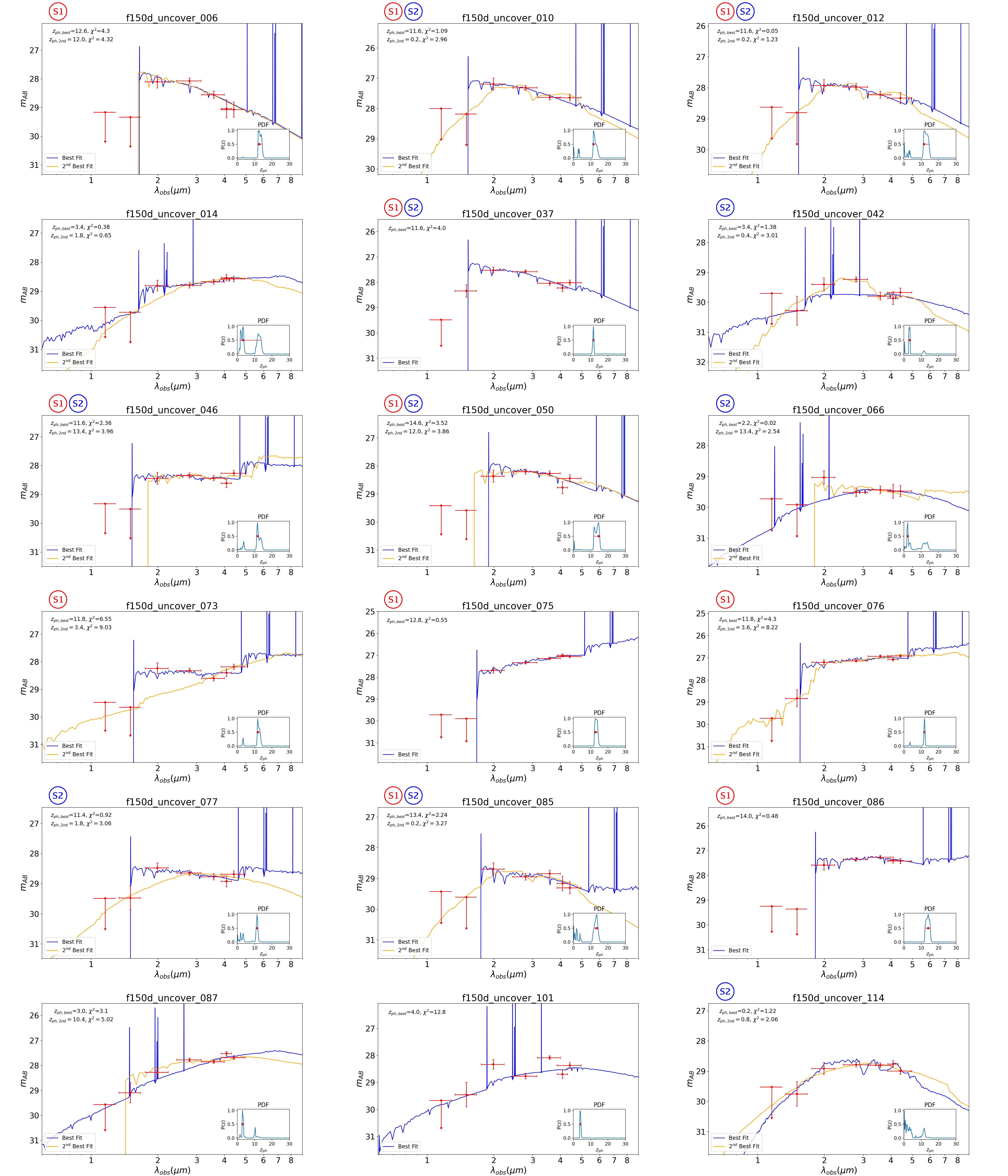
Figure A15: Scheme 1 (S1; using Le Phare and BC03 models) SED fitting results for F150W dropouts in UNCOVER. Each panel shows one F150W dropout, whose SID is labeled to left. The PDF is shown in the inset. The blue curve is the spectrum of the best-fit model corresponding to the first peak of the PDF, which also gives $z_{\rm ph}$ as labeled. If the secondary peak exists, the corresponding model spectrum is also shown as the orange curve. If an object is retained in S1 and/or S2, the plot is marked with {\tinyS1}⃝ and/or {\tinyS2}⃝.

The source catalogs of the F150W, F200W and F277W dropouts in our sample are given as tables below. Their NIRCam image cutouts are displayed in Figures A1 through A14, while their SED fitting results are show in Figures A15 through A32, respectively.

=7mm

Table A1: Catalog of F150W dropouts.

SID	R.A.	Decl.	$m_{090}$	$m_{115}$	$m_{150}$	$m_{200}$	$m_{277}$	$m_{335}$	$m_{356}$	$m_{410}$	$m_{444}$	S1	S2
	(degrees)	(degrees)	(mag)	(mag)	(mag)	(mag)	(mag)	(mag)	(mag)	(mag)	(mag)
f150d_cosmos_010	150.0964901	2.1760648	>27.59	>27.64	27.51±0.49	26.65±0.18	26.43±0.06	…	26.58±0.06	26.89±0.14	26.91±0.13	0	1
f150d_cosmos_019	150.1204786	2.1876317	>28.34	>28.32	28.15±0.54	27.35±0.22	27.29±0.08	…	27.18±0.06	27.26±0.12	27.06±0.09	0	0
f150d_cosmos_021	150.0630699	2.1892588	>27.70	>27.68	>27.84	26.75±0.20	26.94±0.09	…	26.98±0.08	27.05±0.15	27.40±0.17	1	1
f150d_cosmos_030	150.0626968	2.2068158	>27.74	>27.73	>27.93	26.63±0.17	26.79±0.08	…	26.7±0.07	27.11±0.17	26.86±0.12	1	0
f150d_cosmos_032	150.1280942	2.2161717	>28.45	>28.47	28.18±0.47	27.37±0.19	27.44±0.07	…	27.4±0.06	27.56±0.14	27.77±0.14	0	1
f150d_cosmos_065	150.1532019	2.2483807	>28.35	>28.40	>28.63	27.28±0.16	27.57±0.07	…	27.35±0.05	27.39±0.11	27.38±0.08	0	0
f150d_cosmos_069	150.1506812	2.2492089	>28.48	>28.53	>28.76	27.60±0.20	27.65±0.07	…	27.66±0.07	27.70±0.13	27.91±0.12	1	1
f150d_cosmos_075	150.1121016	2.2578627	>28.38	>28.39	>28.58	27.66±0.21	27.79±0.08	…	27.94±0.09	28.19±0.22	27.95±0.15	1	1
f150d_cosmos_105	150.0780525	2.293364	>28.12	>28.18	28.21±0.52	27.28±0.18	27.39±0.08	…	27.70±0.10	27.82±0.21	28.00±0.20	1	1
f150d_cosmos_128	150.118757	2.3147096	>28.54	>28.56	28.41±0.49	27.53±0.18	27.49±0.06	…	27.59±0.06	28.02±0.17	27.66±0.10	1	1
f150d_cosmos_133	150.1411515	2.3181771	>28.67	>28.68	>28.89	27.72±0.21	28.00±0.10	…	27.88±0.08	28.15±0.19	28.01±0.14	1	1
f150d_cosmos_135	150.1729282	2.3184522	>28.46	>28.46	>28.68	27.57±0.20	27.83±0.09	…	27.97±0.09	28.03±0.17	28.26±0.17	1	1
f150d_cosmos_142	150.186187	2.3270214	>28.34	>28.38	27.92±0.38	27.07±0.14	26.73±0.04	…	26.75±0.04	26.63±0.06	26.72±0.05	0	0
f150d_cosmos_143	150.1150419	2.3277913	>28.68	>28.68	>28.89	27.88±0.16	28.00±0.07	…	28.30±0.08	28.26±0.14	28.20±0.11	1	1
f150d_cosmos_161	150.1981908	2.3418706	>27.73	>27.73	>27.94	27.11±0.19	26.95±0.07	…	27.31±0.08	27.42±0.16	27.33±0.12	0	1
f150d_cosmos_208	150.1794883	2.3745223	>28.28	>28.33	>28.51	27.61±0.21	28.23±0.12	…	28.25±0.11	28.74±0.33	28.45±0.20	0	1
f150d_cosmos_217	150.0637146	2.3796138	>27.69	>27.65	>27.85	26.57±0.19	26.55±0.07	…	26.51±0.06	26.81±0.14	26.54±0.10	1	0
f150d_cosmos_228	150.1798098	2.3888704	>28.11	>28.15	27.66±0.49	26.60±0.15	26.38±0.05	…	26.39±0.04	26.67±0.10	26.40±0.06	1	1
f150d_cosmos_238	150.1795179	2.3978379	>28.32	>28.34	>28.58	27.56±0.18	27.93±0.09	…	28.01±0.09	28.09±0.18	28.16±0.15	1	1
f150d_cosmos_247	150.1132498	2.4067704	>28.41	>28.46	>28.49	27.23±0.18	27.37±0.06	…	27.34±0.05	27.21±0.11	27.35±0.09	1	0
f150d_cosmos_265	150.1568953	2.419015	>28.28	>28.30	>28.49	26.61±0.12	26.26±0.03	…	26.05±0.02	26.21±0.05	26.03±0.03	1	0
f150d_cosmos_287	150.1323377	2.4418425	>28.22	>28.21	28.08±0.51	27.22±0.19	27.26±0.08	…	27.21±0.07	27.5±0.16	27.29±0.11	1	1
f150d_cosmos_309	150.1693524	2.4757285	>27.76	>27.75	>27.93	26.87±0.20	27.12±0.10	…	27.15±0.09	27.50±0.21	27.33±0.15	1	1
f150d_uds1_036	34.3652678	$-$5.2949565	>28.45	>28.43	>28.64	27.27±0.19	27.22±0.09	…	26.77±0.05	26.9±0.11	27.01±0.11	0	0
f150d_uds1_037	34.3207228	$-$5.2923562	>28.05	>28.08	>28.25	27.38±0.21	27.73±0.11	…	27.58±0.09	27.96±0.23	27.61±0.15	0	1
f150d_uds1_111	34.3568289	$-$5.253295	>28.27	>28.30	>28.51	27.09±0.19	27.06±0.07	…	26.84±0.06	27.22±0.15	26.69±0.08	1	0
f150d_uds1_124	34.3381297	$-$5.2463882	>28.21	>28.23	28.42±0.51	27.57±0.19	27.83±0.09	…	27.77±0.08	27.64±0.14	28.17±0.19	0	0
f150d_uds1_131	34.3426673	$-$5.2391974	>27.93	>27.96	>28.16	27.34±0.21	27.57±0.09	…	27.54±0.08	27.57±0.17	27.64±0.15	0	1
f150d_uds1_140	34.319141	$-$5.2301575	>28.03	>28.09	>28.28	26.77±0.2	26.82±0.08	…	26.64±0.07	26.75±0.14	26.74±0.11	1	0
f150d_uds1_155	34.2670458	$-$5.2243054	>27.54	>27.61	>27.82	26.41±0.17	26.26±0.05	…	26.34±0.05	26.35±0.11	26.50±0.10	1	1
f150d_uds1_157	34.3275129	$-$5.223183	>28.02	>28.05	>28.25	27.44±0.21	27.66±0.09	…	27.58±0.08	27.94±0.22	27.77±0.16	0	1
f150d_uds1_168	34.3827155	$-$5.2106767	>27.85	>27.87	27.82±0.46	26.99±0.18	27.31±0.07	…	27.42±0.08	27.61±0.18	27.65±0.15	0	1
f150d_uds1_170	34.3516687	$-$5.2068724	>27.58	>27.66	28.16±0.51	27.28±0.19	27.81±0.11	…	28.18±0.14	27.89±0.23	28.26±0.26	0	1
f150d_uds1_178	34.3365264	$-$5.202591	>27.48	>27.54	27.23±0.46	26.24±0.15	26.42±0.06	…	26.46±0.06	26.53±0.13	26.25±0.08	1	1
f150d_uds1_179	34.3556961	$-$5.2008919	>27.54	>27.57	>27.80	26.86±0.21	27.24±0.09	…	27.10±0.08	27.61±0.25	27.58±0.19	0	1
f150d_uds1_180	34.3419743	$-$5.2002854	>27.53	>27.52	27.52±0.35	26.71±0.14	26.56±0.04	…	26.32±0.03	26.33±0.06	26.30±0.05	0	0
f150d_uds1_189	34.4532399	$-$5.1642041	>27.62	>27.64	27.79±0.49	26.95±0.18	27.16±0.08	…	27.14±0.07	27.16±0.15	27.21±0.12	0	1
f150d_uds1_191	34.3380838	$-$5.1555267	>28.00	>28.03	>28.24	27.26±0.17	27.88±0.11	…	27.97±0.10	28.02±0.20	27.91±0.15	0	1
f150d_ceers_003	215.0163153	52.8707935	…	>29.48	>29.00	27.68±0.19	27.68±0.08	…	27.54±0.06	27.57±0.14	27.45±0.11	0	0
f150d_ceers_014	214.8103744	52.7397808	…	>29.12	28.33±0.49	27.39±0.17	27.17±0.06	…	27.24±0.06	27.07±0.10	27.0±0.08	1	0
f150d_ceers_031	215.0666659	52.9333503	…	>29.30	>28.87	27.24±0.17	27.42±0.07	…	27.23±0.05	27.42±0.15	27.25±0.10	1	0
f150d_ceers_041	214.7737282	52.7404111	…	>29.05	>28.85	28.01±0.19	27.63±0.05	…	27.38±0.04	27.25±0.07	27.42±0.07	0	0
f150d_ceers_046	214.9739734	52.8847591	…	>29.29	>28.85	27.95±0.21	28.29±0.11	…	28.25±0.08	28.76±0.32	28.12±0.15	0	1
f150d_ceers_051	214.8876228	52.8296748	…	>29.05	28.67±0.42	27.84±0.15	27.53±0.04	…	27.64±0.05	27.54±0.08	27.47±0.06	0	0
f150d_ceers_060	214.941266	52.8805983	…	>29.44	27.82±0.33	26.98±0.13	27.27±0.07	…	27.18±0.05	27.33±0.14	27.23±0.11	1	1
f150d_ceers_079	214.9082292	52.8968555	…	>29.03	28.69±0.47	27.74±0.16	27.61±0.06	…	27.80±0.06	28.07±0.16	27.96±0.13	1	1
f150d_ceers_087	214.8740717	52.876717	…	>28.90	>28.70	27.39±0.14	26.92±0.05	…	27.29±0.06	27.51±0.15	27.62±0.10	1	0
f150d_ceers_088	214.8743088	52.8767738	…	>28.91	>28.70	27.73±0.17	27.68±0.09	…	27.87±0.09	27.58±0.14	28.86±0.28	0	0
f150d_ceers_089	214.9320161	52.9182491	…	>28.92	>28.79	27.86±0.20	27.82±0.10	…	27.64±0.08	27.69±0.17	27.71±0.10	0	0
f150d_ceers_125	214.9431552	52.9424513	…	>28.96	>28.95	27.98±0.15	28.34±0.09	…	28.41±0.09	28.48±0.19	28.28±0.13	0	1
f150d_ceers_150	214.9849543	52.990391	…	>29.09	>28.92	27.89±0.18	27.74±0.07	…	27.75±0.07	28.01±0.16	28.21±0.16	1	1
f150d_ceers_153	214.8567793	52.9030729	…	>28.95	>28.80	27.77±0.18	27.76±0.08	…	27.76±0.08	27.99±0.17	27.66±0.11	1	1
f150d_ceers_161	214.9066563	52.9455063	…	>29.00	>28.83	27.48±0.18	27.32±0.06	…	27.20±0.05	27.21±0.10	27.15±0.08	1	0
f150d_glass_003	3.5140762	$-$30.3839153	>29.66	>29.62	>29.42	28.29±0.20	27.56±0.05	…	27.24±0.03	…	27.01±0.02	0	0
f150d_glass_024	3.4915046	$-$30.362516	>29.91	>29.89	>29.43	28.39±0.20	27.87±0.05	…	27.81±0.05	…	27.83±0.04	1	0
f150d_glass_029	3.5321168	$-$30.3614222	>29.83	>29.83	>29.63	28.76±0.21	28.93±0.10	…	28.25±0.05	…	28.27±0.04	0	0
f150d_glass_039	3.5135577	$-$30.3567969	>29.95	>29.95	>29.76	28.43±0.15	28.91±0.08	…	29.24±0.10	…	30.30±0.21	0	0
f150d_glass_067	3.4506757	$-$30.331406	>29.57	>29.59	>29.39	27.62±0.17	27.07±0.04	…	27.07±0.04	…	26.86±0.03	1	0
f150d_glass_075	3.4989394	$-$30.3253288	>29.87	>29.72	>29.69	28.38±0.19	28.47±0.09	…	28.38±0.07	…	28.39±0.06	1	0
f150d_glass_076	3.4989889	$-$30.3247604	>29.88	>29.75	28.69±0.38	26.7±0.05	27.04±0.03	…	27.09±0.03	…	27.10±0.02	0	0
f150d_ngdeep_014	53.2515487	$-$27.8571346	…	>30.56	>30.32	29.29±0.14	30.74±0.20	…	30.28±0.13	…	30.55±0.19	0	0
f150d_ngdeep_018	53.2769065	$-$27.8505161	…	>30.56	29.15±0.21	28.15±0.12	28.74±0.05	…	28.49±0.05	…	28.84±0.06	0	0
f150d_ngdeep_034	53.2266642	$-$27.8210254	…	>30.26	29.96±0.46	29.14±0.19	28.7±0.04	…	28.46±0.03	…	28.87±0.05	0	0
f150d_ngdeep_038	53.2383719	$-$27.8153782	…	>30.55	30.43±0.45	29.46±0.18	30.39±0.14	…	30.24±0.13	…	30.33±0.16	0	1
f150d_jades_A1_005	53.1115765	$-$27.8108276	>30.21	>30.61	>30.41	29.45±0.14	29.42±0.05	29.60±0.08	29.53±0.05	30.00±0.15	29.94±0.12	1	1
f150d_jades_A1_007	53.1113635	$-$27.8075635	>30.21	>30.61	30.91±0.54	29.90±0.17	30.62±0.12	30.44±0.13	30.19±0.07	30.73±0.23	30.83±0.21	0	0
f150d_jades_A1_008	53.1686016	$-$27.7939249	>30.57	>30.82	31.12±0.43	30.21±0.21	30.89±0.11	>31.38	30.48±0.09	31.3±0.27	30.89±0.16	0	0
f150d_jades_A1_009	53.1686315	$-$27.7927587	>30.57	>30.82	30.40±0.28	29.23±0.11	29.39±0.03	29.59±0.08	29.57±0.05	29.83±0.09	29.77±0.07	1	1
f150d_jades_A1_012	53.1570142	$-$27.7896965	>30.65	>30.95	31.30±0.38	30.38±0.19	30.77±0.08	>31.42	30.50±0.08	31.82±0.37	30.76±0.12	0	0
f150d_jades_A1_018	53.1801703	$-$27.7801054	>30.37	>30.72	29.31±0.29	28.38±0.10	27.96±0.03	27.92±0.04	27.78±0.02	27.78±0.04	28.05±0.05	0	0
f150d_jades_A1_019	53.1803562	$-$27.7800919	>30.37	>30.73	29.72±0.46	27.97±0.08	27.67±0.03	27.61±0.03	27.62±0.02	27.69±0.04	27.51±0.03	1	0
f150d_jades_A2_001	53.1685698	$-$27.8421018	>30.23	>30.65	30.34±0.35	29.23±0.10	30.35±0.11	30.61±0.18	29.82±0.06	30.34±0.19	29.58±0.08	0	0
f150d_jades_A2_002	53.1504747	$-$27.8350217	>30.23	>30.61	>30.43	29.43±0.15	29.14±0.04	29.24±0.07	28.99±0.04	29.03±0.07	29.14±0.06	1	0
f150d_jades_A2_006	53.166346	$-$27.8215581	>30.87	>31.18	31.03±0.51	29.21±0.09	29.07±0.03	29.4±0.06	29.16±0.03	29.24±0.05	29.37±0.05	0	0
f150d_jades_A2_008	53.158609	$-$27.8147378	>30.79	>31.10	30.91±0.33	29.96±0.13	30.44±0.06	30.52±0.11	30.33±0.06	30.80±0.15	30.57±0.10	0	1
f150d_jades_A2_009	53.1662719	$-$27.8137652	>30.71	>31.05	31.62±0.50	30.35±0.14	31.14±0.09	31.00±0.12	30.85±0.07	30.64±0.10	30.91±0.10	0	0
f150d_jades_A2_015	53.1428281	$-$27.8080515	>30.86	>31.18	31.62±0.44	30.73±0.19	31.19±0.09	30.98±0.13	31.15±0.10	31.57±0.23	31.27±0.15	0	1
f150d_jades_A2_016	53.1612338	$-$27.8074642	>30.78	>31.08	31.15±0.44	30.24±0.19	30.54±0.07	30.33±0.10	30.08±0.06	30.39±0.11	30.37±0.09	0	0
f150d_jades_A2_021	53.195856	$-$27.789175	>30.36	>30.70	30.53±0.47	29.62±0.16	29.86±0.09	29.57±0.09	29.37±0.05	30.05±0.17	30.49±0.22	0	0
f150d_jades_A2_027	53.2148161	$-$27.7743605	>30.86	>31.15	31.90±0.50	31.03±0.21	31.81±0.16	32.50±0.44	31.37±0.10	32.17±0.36	32.01±0.28	0	0
f150d_jades_A2_030	53.1899349	$-$27.7714981	>30.90	>31.17	30.42±0.22	29.43±0.09	30.00±0.05	30.11±0.09	30.14±0.06	30.36±0.12	30.71±0.14	1	0
f150d_jades_A2_035	53.1811069	$-$27.7567872	>30.96	>31.21	>31.16	29.87±0.16	29.67±0.05	30.15±0.11	29.76±0.05	29.42±0.06	29.63±0.06	0	0
f150d_jades_A2_038	53.1805623	$-$27.7454842	>30.70	>30.90	30.48±0.28	29.51±0.13	29.90±0.06	29.91±0.11	29.92±0.07	30.14±0.11	30.66±0.16	0	0
f150d_jades_A2_042	53.1999861	$-$27.7594299	>30.70	>30.77	31.06±0.50	29.88±0.17	30.44±0.08	30.94±0.24	30.16±0.08	31.32±0.29	31.41±0.28	0	0
f150d_uncover_006	3.5870168	$-$30.4334048	…	>29.16	>29.33	28.10±0.21	28.07±0.09	…	28.55±0.12	29.04±0.31	29.07±0.26	1	0
f150d_uncover_010	3.6577825	$-$30.4271833	…	>28.00	>28.18	27.19±0.19	27.31±0.06	…	27.63±0.07	…	27.64±0.10	1	1
f150d_uncover_012	3.6159364	$-$30.4251697	…	>28.62	>28.80	27.92±0.18	27.97±0.09	…	28.22±0.10	…	28.33±0.17	1	1
f150d_uncover_014	3.5874615	$-$30.4228282	…	>29.55	>29.72	28.80±0.18	28.79±0.08	…	28.67±0.07	28.53±0.10	28.57±0.08	0	0
f150d_uncover_037	3.563056	$-$30.4080157	…	>29.48	28.34±0.24	27.52±0.11	27.58±0.05	…	28.03±0.07	28.22±0.14	28.01±0.09	1	1
f150d_uncover_042	3.6048043	$-$30.402524	…	>29.70	30.28±0.48	29.40±0.21	29.23±0.07	…	29.79±0.12	29.86±0.21	29.67±0.14	0	1
f150d_uncover_046	3.5669842	$-$30.3999489	…	>29.32	>29.50	28.44±0.20	28.34±0.07	…	28.43±0.07	28.61±0.14	28.26±0.08	1	1
f150d_uncover_050	3.5695468	$-$30.3956585	…	>29.41	>29.58	28.36±0.21	28.20±0.08	…	28.26±0.08	28.77±0.21	28.44±0.12	1	1
f150d_uncover_066	3.5320761	$-$30.3856738	…	>29.72	>29.91	29.03±0.21	29.51±0.13	…	29.43±0.11	29.48±0.22	29.47±0.17	0	1
f150d_uncover_073	3.5489514	$-$30.3826595	…	>29.47	>29.65	28.24±0.19	28.32±0.07	…	28.60±0.08	28.40±0.13	28.18±0.08	1	0
f150d_uncover_075	3.5408473	$-$30.3806381	…	>29.71	>29.89	27.68±0.13	27.33±0.04	…	27.14±0.03	27.00±0.05	27.05±0.04	1	0
f150d_uncover_076	3.5407993	$-$30.3804695	…	>29.72	28.83±0.38	27.20±0.09	27.13±0.03	…	26.93±0.03	27.07±0.05	26.91±0.04	1	0
f150d_uncover_077	3.5882198	$-$30.380086	…	>29.48	29.47±0.39	28.47±0.15	28.64±0.07	…	28.77±0.09	28.92±0.18	28.68±0.10	0	1
f150d_uncover_085	3.5854814	$-$30.3769822	…	>29.42	>29.60	28.69±0.20	28.94±0.10	…	28.84±0.10	29.16±0.23	29.30±0.19	1	1
f150d_uncover_086	3.5127318	$-$30.3760189	…	>29.24	>29.35	27.58±0.20	27.35±0.06	…	27.26±0.05	27.38±0.11	27.42±0.09	1	0
f150d_uncover_087	3.5998595	$-$30.3752635	…	>29.56	29.09±0.41	28.27±0.19	27.77±0.05	…	27.85±0.05	27.52±0.07	27.68±0.06	0	0
f150d_uncover_101	3.5580068	$-$30.3548082	…	>29.66	29.45±0.45	28.33±0.17	28.76±0.09	…	28.08±0.05	28.69±0.15	28.37±0.09	0	0
f150d_uncover_114	3.5734992	$-$30.3382778	…	>29.52	29.75±0.40	28.91±0.19	28.78±0.06	…	28.80±0.06	28.76±0.10	28.99±0.10	0	1
f150d_smacs0723_A_004	110.6870102	$-$73.4982429	>29.15	…	>29.34	28.46±0.19	28.66±0.08	…	28.69±0.08	…	28.99±0.16	1	1
f150d_smacs0723_A_006	110.6401082	$-$73.4945819	>28.60	…	28.03±0.32	27.1±0.11	26.97±0.04	…	26.99±0.04	…	26.97±0.06	0	1
f150d_smacs0723_A_013	110.7161536	$-$73.4836327	>29.29	…	>29.48	28.51±0.19	28.72±0.1	…	28.7±0.09	…	29.28±0.22	1	1
f150d_smacs0723_A_014	110.7348001	$-$73.4834393	>29.30	…	29.4±0.46	28.52±0.18	28.8±0.09	…	28.96±0.1	…	28.88±0.14	0	1
f150d_smacs0723_A_015	110.66939	$-$73.4834712	>29.26	…	>29.42	28.46±0.21	28.6±0.1	…	28.57±0.09	…	28.75±0.15	1	1
f150d_smacs0723_A_020	110.6401283	$-$73.4800748	>29.27	…	>29.42	27.17±0.13	27.07±0.05	…	26.96±0.04	…	27.15±0.07	1	0
f150d_smacs0723_A_022	110.6875291	$-$73.4769086	>29.31	…	>29.46	27.98±0.17	28.06±0.08	…	27.98±0.07	…	28.38±0.15	1	1
f150d_smacs0723_A_023	110.6025405	$-$73.4749489	>28.65	…	28.68±0.44	27.85±0.18	28.35±0.1	…	28.71±0.14	…	28.57±0.18	0	0
f150d_smacs0723_A_024	110.6716036	$-$73.4744491	>29.24	…	29.5±0.49	28.62±0.18	29.14±0.13	…	28.93±0.1	…	28.94±0.14	0	0
f150d_smacs0723_A_026	110.6598067	$-$73.4658505	>29.07	…	>29.23	28.39±0.21	28.65±0.11	…	28.45±0.09	…	28.5±0.13	0	1
f150d_smacs0723_A_028	110.6909711	$-$73.4631649	>29.29	…	28.92±0.4	27.95±0.13	27.74±0.05	…	27.99±0.06	…	28.08±0.09	0	1
f150d_smacs0723_A_029	110.682593	$-$73.4587622	>28.68	…	28.73±0.46	27.88±0.17	27.88±0.07	…	28.07±0.08	…	27.87±0.1	0	1
f150d_smacs0723_B_005	110.8540062	$-$73.4647108	>28.89	…	28.55±0.33	27.62±0.12	28.2±0.06	…	28.71±0.09	…	29.99±0.43	0	0
f150d_smacs0723_B_009	110.835143	$-$73.4631564	>29.15	…	28.95±0.42	27.93±0.14	27.95±0.05	…	28.2±0.06	…	28.22±0.09	0	1
f150d_smacs0723_B_019	110.7565239	$-$73.4549995	>29.04	…	28.2±0.49	26.96±0.13	27.16±0.06	…	26.97±0.06	…	26.94±0.08	0	0
f150d_smacs0723_B_028	110.8117102	$-$73.4494943	>29.20	…	29.58±0.47	28.71±0.18	29.1±0.1	…	29.36±0.12	…	>30.28	0	1
f150d_smacs0723_B_033	110.7961874	$-$73.4446427	>29.03	…	29.1±0.48	28.24±0.18	28.79±0.1	…	29.07±0.12	…	29.21±0.21	0	1
f150d_smacs0723_B_034	110.8377757	$-$73.4410561	>29.17	…	27.94±0.29	27.13±0.11	26.83±0.03	…	26.82±0.03	…	27.08±0.06	0	1
f150d_smacs0723_B_036	110.8711286	$-$73.4408142	>28.93	…	28.92±0.5	27.74±0.14	28.06±0.07	…	27.93±0.06	…	28.09±0.1	0	1
f150d_smacs0723_B_038	110.8084692	$-$73.4381453	>29.17	…	29.63±0.39	28.43±0.11	28.38±0.04	…	28.41±0.04	…	28.43±0.06	1	1
f150d_smacs0723_B_039	110.8130436	$-$73.4362453	>28.95	…	>29.19	27.34±0.19	27.27±0.07	…	27.09±0.06	…	27.48±0.12	1	0

Note. — Basic information of the JWST Cycle 1 public NIRCam data used in this study. The blank fields and the cluster fields are separated by the horizontal line. The listed coordinates are for the central positions of the final mosaics. The exposure times (in kilo-seconds) are representative estimates. The external catalogs used for astrometric calibration and image alignment are listed in the last column.

Note. — For the F150W and F200W dropouts, the number of objects after the purification in Scheme 1 and 2 are also listed separately. The F277W dropouts are not purified due to the limited SED information.

Note. — The faint-end values of these luminosity functions are not reliable due to the selection limits (see Section 6.4). These happen at $M_{UV}>-18.1$ mag and $>-19.1$ mag for $z\approx 12.7$ and 17.3, respectively.

Note. — SID is the unique identifier of a given F150W dropout, which has the field of discovery encoded. R.A. and Decl. are of J2000.0 equinox. All magnitudes are SExtractor’s MAG_ISO whose aperture is defined in the F356W image. Columns S1 and S2 contain the flags of the purification in S1 and S2, where “1” means that the given dropout is retained and “0” means that it is rejected.

Table A2: Photometry table for F200W dropouts.

SID	R.A.	Decl.	$m_{090}$	$m_{115}$	$m_{150}$	$m_{200}$	$m_{277}$	$m_{335}$	$m_{356}$	$m_{410}$	$m_{444}$	S1	S2
	(degrees)	(degrees)	(mag)	(mag)	(mag)	(mag)	(mag)	(mag)	(mag)	(mag)	(mag)
f200d_cosmos_032	150.1550473	2.2428093	>27.79	>27.82	>28.01	>28.28	27.29±0.08	…	27.16±0.06	27.10±0.11	27.30±0.11	1	1
f200d_cosmos_043	150.109837	2.2578077	>28.41	>28.43	>28.62	28.06±0.47	27.25±0.08	…	26.62±0.05	26.23±0.06	25.96±0.04	0	0
f200d_cosmos_065	150.0990525	2.287338	>28.25	>28.26	>28.44	29.08±0.53	28.27±0.08	…	28.68±0.12	28.35±0.17	28.95±0.23	0	1
f200d_cosmos_067	150.1653459	2.2885879	>28.16	>28.17	>28.39	>28.64	27.52±0.11	…	27.16±0.07	27.98±0.28	27.81±0.19	0	1
f200d_cosmos_079	150.1566124	2.3008789	>28.17	>28.19	>28.43	>28.62	27.72±0.08	…	27.58±0.06	27.78±0.14	27.69±0.11	1	1
f200d_cosmos_096	150.0921291	2.3270286	>28.11	>28.13	>28.34	>28.54	27.64±0.10	…	27.50±0.08	27.88±0.21	27.51±0.12	1	1
f200d_cosmos_099	150.1325098	2.328851	>28.76	>28.77	>28.99	>29.19	28.28±0.10	…	28.07±0.08	28.39±0.19	28.29±0.14	1	1
f200d_cosmos_131	150.1942323	2.3715004	>27.73	>27.71	>27.89	>28.12	27.11±0.11	…	26.99±0.08	26.99±0.15	27.25±0.15	1	1
f200d_cosmos_142	150.1752034	2.3844173	>28.10	>28.11	>28.30	>28.52	27.52±0.14	…	27.10±0.08	27.36±0.19	27.57±0.18	0	1
f200d_cosmos_166	150.1012306	2.4185747	>27.92	>27.97	>28.19	27.43±0.41	26.56±0.06	…	26.35±0.05	26.40±0.09	26.59±0.09	0	1
f200d_cosmos_167	150.1558489	2.4225843	>28.40	>28.43	>28.64	28.41±0.48	27.45±0.08	…	27.26±0.06	27.31±0.12	27.26±0.09	0	1
f200d_cosmos_168	150.1557862	2.4228785	>28.34	>28.34	>28.57	>28.76	26.80±0.05	…	26.59±0.04	26.33±0.06	26.69±0.06	1	1
f200d_cosmos_175	150.107368	2.4287796	>27.63	>27.68	>27.90	>28.09	26.69±0.08	…	26.49±0.06	26.39±0.11	26.49±0.09	1	1
f200d_cosmos_181	150.1044823	2.4354193	>27.53	>27.62	>27.88	>28.04	27.21±0.14	…	26.15±0.05	25.99±0.08	25.79±0.05	0	1
f200d_cosmos_191	150.1207149	2.4701671	>27.64	>27.64	>27.84	>28.06	26.72±0.08	…	26.32±0.05	26.16±0.07	26.13±0.06	0	1
f200d_uds1_003	34.2430186	$-$5.319367	>27.67	>27.63	>27.85	>28.09	27.07±0.09	…	26.27±0.04	26.27±0.07	26.25±0.06	0	1
f200d_uds1_013	34.4008915	$-$5.3110921	>27.57	>27.53	>27.76	>27.96	27.13±0.07	…	27.31±0.08	26.38±0.06	27.09±0.10	0	0
f200d_uds1_057	34.3013215	$-$5.2880627	>27.82	>27.82	>28.02	27.49±0.41	26.51±0.05	…	26.35±0.04	26.57±0.09	26.53±0.08	0	0
f200d_uds1_058	34.3008324	$-$5.2879215	>27.99	>27.99	>28.18	>28.42	26.69±0.07	…	26.19±0.04	26.71±0.12	26.61±0.09	1	1
f200d_uds1_071	34.3787906	$-$5.2821969	>28.10	>28.10	>28.29	28.39±0.5	27.40±0.08	…	27.74±0.10	27.79±0.20	27.86±0.18	0	1
f200d_uds1_077	34.2324197	$-$5.2806268	>28.13	>28.08	>28.28	>28.52	27.65±0.10	…	26.75±0.04	26.81±0.08	26.48±0.05	0	1
f200d_uds1_078	34.5031519	$-$5.2796558	>28.06	>28.08	>28.26	27.53±0.27	26.70±0.05	…	26.80±0.05	27.07±0.12	27.06±0.10	1	1
f200d_uds1_089	34.3760515	$-$5.2717343	>28.02	>28.01	>28.24	>28.47	27.58±0.09	…	27.51±0.08	27.68±0.18	27.56±0.14	1	1
f200d_uds1_105	34.3747928	$-$5.2608881	>28.07	>28.06	>28.26	28.36±0.47	27.54±0.09	…	27.80±0.10	28.48±0.38	28.42±0.29	0	1
f200d_uds1_107	34.3890922	$-$5.2591026	>28.58	>28.56	>28.78	>29.01	28.20±0.09	…	28.42±0.11	29.06±0.38	28.94±0.28	1	1
f200d_uds1_115	34.5019208	$-$5.2521015	>27.94	>27.97	>28.23	>28.42	27.51±0.07	…	28.01±0.10	>29.15	28.30±0.20	0	1
f200d_uds1_116	34.3727848	$-$5.2520965	>28.22	>28.27	>28.47	>28.67	27.25±0.09	…	27.30±0.09	27.87±0.32	28.64±0.53	1	1
f200d_uds1_119	34.3552164	$-$5.2489235	>28.27	>28.30	>28.50	>28.72	27.73±0.08	…	27.86±0.09	28.27±0.26	28.13±0.19	1	1
f200d_uds1_158	34.2469537	$-$5.2112719	>27.60	>27.58	>27.85	>28.08	27.04±0.11	…	26.64±0.07	26.89±0.19	26.72±0.13	1	1
f200d_uds1_175	34.3495507	$-$5.1520157	>28.08	>28.09	>28.32	>28.50	27.34±0.08	…	27.55±0.09	28.39±0.35	27.68±0.15	1	1
f200d_ceers_008	215.0921882	52.9199048	…	>29.37	>28.91	28.23±0.42	27.03±0.05	…	26.69±0.03	26.72±0.08	26.73±0.07	0	1
f200d_ceers_054	214.8506944	52.7769011	…	>29.14	>28.95	>29.15	28.24±0.13	…	28.03±0.09	27.59±0.12	27.88±0.14	0	1
f200d_ceers_068	215.1373846	52.9885643	…	>29.32	>28.84	>29.06	28.20±0.10	…	28.10±0.07	28.02±0.16	28.28±0.18	1	1
f200d_glass_001	3.5142827	$-$30.3837111	>29.67	>29.64	>29.42	>29.63	28.27±0.09	…	28.35±0.08	…	28.74±0.10	1	1
f200d_glass_008	3.5087307	$-$30.3767261	>29.90	>29.88	>29.69	>29.89	28.71±0.11	…	28.83±0.11	…	29.23±0.13	1	1
f200d_glass_023	3.5274208	$-$30.367695	>29.83	>29.86	>29.66	>29.83	27.94±0.07	…	27.84±0.06	…	27.80±0.05	1	1
f200d_glass_025	3.5234561	$-$30.3667739	>29.83	>29.85	>29.67	30.01±0.50	28.90±0.07	…	29.65±0.12	…	29.21±0.07	0	0
f200d_glass_064	3.4970253	$-$30.3498509	>29.93	>29.89	>29.71	27.83±0.20	26.96±0.04	…	26.97±0.03	…	27.11±0.03	0	0
f200d_glass_084	3.4767446	$-$30.325534	>29.87	>29.87	>29.39	>29.89	29.00±0.13	…	28.59±0.10	…	29.20±0.11	0	1
f200d_ngdeep_004	53.2494577	$-$27.8756523	…	>30.86	>30.62	30.08±0.36	29.27±0.06	…	29.30±0.06	…	29.55±0.09	0	0
f200d_jades_A1_008	53.1677942	$-$27.768485	>30.69	>30.86	>30.84	>30.71	29.54±0.04	30.08±0.11	29.57±0.05	30.32±0.14	30.27±0.12	0	0
f200d_jades_A2_001	53.172829	$-$27.8415601	>30.25	>30.65	>30.46	>30.70	29.88±0.07	30.57±0.17	29.89±0.06	30.43±0.20	30.70±0.21	0	0
f200d_jades_A2_010	53.1269214	$-$27.7910264	>30.79	>31.10	>31.00	30.69±0.32	29.76±0.04	29.37±0.05	29.35±0.03	29.60±0.06	29.58±0.05	0	1
f200d_jades_A2_011	53.2005513	$-$27.7849306	>30.68	>30.88	>30.82	>30.74	29.41±0.04	29.31±0.06	28.90±0.03	29.70±0.09	29.47±0.06	0	0
f200d_uncover_024	3.6338542	$-$30.4374596	…	>28.29	>28.45	>28.65	27.60±0.10	…	27.68±0.09	…	28.02±0.21	0	1
f200d_uncover_147	3.6344337	$-$30.3988995	…	>28.83	>28.89	29.01±0.51	28.10±0.09	…	28.47±0.11	28.74±0.31	28.67±0.19	0	1
f200d_uncover_189	3.5618012	$-$30.3879883	…	>29.09	>29.30	>29.29	28.31±0.10	…	28.02±0.07	28.23±0.16	28.90±0.23	0	1
f200d_uncover_333	3.5782373	$-$30.3309647	…	>29.16	>29.42	>29.42	28.38±0.09	…	28.72±0.11	29.49±0.41	29.15±0.24	1	1
f200d_smacs0723_A_004	110.7335419	$-$73.4894246	>29.27	…	>29.46	>29.66	28.47±0.14	…	27.73±0.07	…	27.93±0.12	0	1
f200d_smacs0723_A_013	110.7067627	$-$73.4743838	>29.25	…	>29.41	28.68±0.47	27.58±0.07	…	27.36±0.05	…	27.38±0.08	0	1
f200d_smacs0723_B_010	110.8019147	$-$73.4572911	>29.00	…	>29.21	>29.37	28.45±0.09	…	28.14±0.06	…	28.59±0.14	1	1
f200d_smacs0723_B_023	110.8026074	$-$73.442157	>28.96	…	>29.21	29.01±0.54	28.20±0.08	…	28.28±0.08	…	28.84±0.20	0	1

Note. — Similar to Table A1 but for the F200W dropouts.

Table A3: Photometry table for F277W dropouts.

SID	R.A.	Decl.	$m_{090}$	$m_{115}$	$m_{150}$	$m_{200}$	$m_{277}$	$m_{335}$	$m_{356}$	$m_{410}$	$m_{444}$
	(degrees)	(degrees)	(mag)	(mag)	(mag)	(mag)	(mag)	(mag)	(mag)	(mag)	(mag)
f277d_cosmos_026	150.1047951	2.264002	>27.98	>27.96	>28.20	>28.40	28.89±0.17	…	27.67±0.06	27.45±0.10	27.21±0.07
f277d_cosmos_038	150.0917946	2.2896575	>28.06	>28.05	>28.26	>28.47	28.74±0.20	…	27.91±0.10	27.64±0.15	27.39±0.10
f277d_cosmos_083	150.1319202	2.3999325	>28.54	>28.58	>28.65	>28.84	>30.14	…	29.04±0.12	28.63±0.18	28.83±0.17
f277d_cosmos_091	150.1044624	2.4353101	>27.55	>27.64	>27.85	>28.07	28.67±0.32	…	27.29±0.09	27.15±0.15	26.77±0.08
f277d_cosmos_092	150.1044823	2.4354193	>27.53	>27.62	>27.88	>28.04	27.21±0.14	…	26.15±0.05	25.99±0.08	25.79±0.05
f277d_cosmos_099	150.1510552	2.4737863	>27.76	>27.72	>27.90	>28.25	29.27±0.48	…	27.93±0.12	27.5±0.15	28.17±0.22
f277d_uds1_003	34.4769352	$-$5.3142233	>27.70	>27.67	>27.86	>28.10	28.73±0.31	…	26.84±0.05	26.12±0.05	26.04±0.04
f277d_uds1_011	34.3655349	$-$5.2856743	>28.10	>28.08	>28.30	>28.51	>29.51	…	28.12±0.10	27.22±0.09	27.05±0.07
f277d_uds1_040	34.4850689	$-$5.2455844	>28.28	>28.34	>28.53	>28.72	29.34±0.28	…	28.43±0.11	28.65±0.28	28.22±0.16
f277d_uds1_056	34.4737407	$-$5.2176787	>28.19	>28.21	>28.44	>28.64	29.76±0.45	…	27.82±0.08	27.24±0.09	27.44±0.08
f277d_uds1_064	34.3358389	$-$5.2014531	>27.51	>27.57	>27.77	>27.98	29.43±0.44	…	28.23±0.14	28.92±0.58	27.66±0.14
f277d_uds1_069	34.3523512	$-$5.1816831	>27.93	>27.97	>28.19	>28.42	>29.63	…	28.79±0.15	26.88±0.06	26.93±0.04
f277d_uds1_077	34.4294851	$-$5.1288507	>27.77	>27.70	>27.92	>28.12	28.11±0.22	…	27.16±0.08	26.42±0.08	26.66±0.08
f277d_ceers_022	214.9298649	52.8072661	…	>29.62	>28.96	>29.22	29.47±0.29	…	28.01±0.06	27.65±0.11	27.68±0.07
f277d_ceers_095	214.8057858	52.7347332	…	>29.11	>28.93	>29.14	29.39±0.25	…	28.56±0.11	29.17±0.39	29.20±0.33
f277d_ceers_485	214.7148366	52.7434037	…	>29.06	>28.87	>29.07	29.67±0.29	…	28.51±0.10	27.91±0.12	27.94±0.10
f277d_glass_007	3.4891744	$-$30.3645975	>29.69	…	>29.41	>29.67	30.33±0.32	…	29.44±0.13	…	30.20±0.21
f277d_glass_011	3.4949794	$-$30.3614903	>29.92	…	>29.71	>29.91	>30.90	…	29.91±0.17	…	29.83±0.13
f277d_ngdeep_012	53.2519601	$-$27.8732495	…	>30.86	>30.63	>30.68	31.72±0.44	…	30.49±0.15	…	30.46±0.16
f277d_ngdeep_053	53.2492831	$-$27.824109	…	>30.79	>30.57	>30.63	31.27±0.31	…	30.15±0.11	…	30.48±0.18
f277d_jades_A1_059	53.1622288	$-$27.8025417	>30.23	>30.63	>30.44	>30.67	31.98±0.21	31.03±0.14	30.72±0.07	29.94±0.06	30.28±0.07
f277d_jades_A1_122	53.1777365	$-$27.774737	>30.46	>30.76	>30.60	>30.78	31.95±0.30	>31.68	30.57±0.07	30.73±0.15	31.88±0.40
f277d_jades_A1_125	53.1591677	$-$27.7731353	>30.37	>30.69	>30.49	>30.73	32.03±0.34	32.02±0.47	30.76±0.09	>31.14	31.01±0.18
f277d_jades_A1_993	53.1727658	$-$27.7918711	>30.81	>31.11	>31.02	>31.06	>32.22	31.32±0.18	31.3±0.12	>31.64	>31.81
f277d_jades_A2_056	53.1976644	$-$27.7700823	>30.60	>30.76	>30.73	>30.51	32.32±0.26	31.52±0.19	31.24±0.10	>31.72	>31.83
f277d_jades_A2_064	53.1318805	$-$27.766531	>30.73	>31.03	>30.92	>30.94	31.38±0.24	31.38±0.32	30.38±0.08	>31.19	30.52±0.16
f277d_jades_A2_074	53.1817889	$-$27.7584684	>31.24	>31.51	>31.38	>31.44	>32.48	>32.00	31.26±0.09	30.69±0.08	30.60±0.07
f277d_jades_A2_104	53.1717078	$-$27.7442152	>30.70	>30.90	>30.83	>30.70	32.06±0.28	>31.26	30.73±0.10	31.06±0.17	>31.58
f277d_jades_A2_112	53.172755	$-$27.739298	>30.69	>30.90	>30.82	>30.70	33.10±0.51	31.22±0.17	31.51±0.14	>31.50	>31.64
f277d_jades_A2_118	53.1878657	$-$27.7420226	>30.78	>30.94	>30.90	>30.72	33.38±0.51	32.23±0.33	32.07±0.18	32.43±0.34	31.87±0.18
f277d_uncover_011	3.6369782	$-$30.4211829	…	>28.63	>28.83	>29.05	27.09±0.08	…	25.94±0.02	…	25.48±0.03
f277d_smacs0723_B_001	110.78867	$-$73.4559726	>29.26	…	>29.46	>29.62	>30.64	…	29.75±0.15	…	28.78±0.09

Note. — Similar to Table A1 but for the F277W dropouts. Note that these dropouts are not purified due to the limitation in their SEDs.

Figure A1: Similar to Figure 1; for the F150W dropouts in COSMOS.

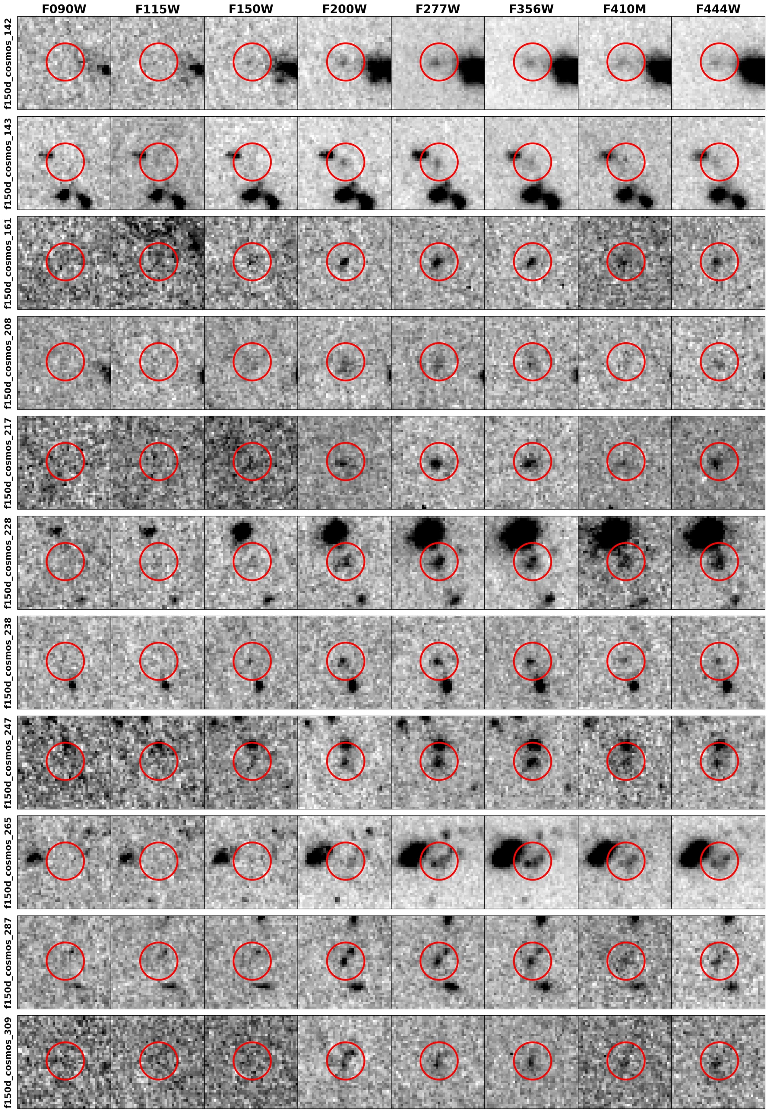
Figure A1 (Cont.): Similar to Figure 1; for the F150W dropouts in COSMOS.

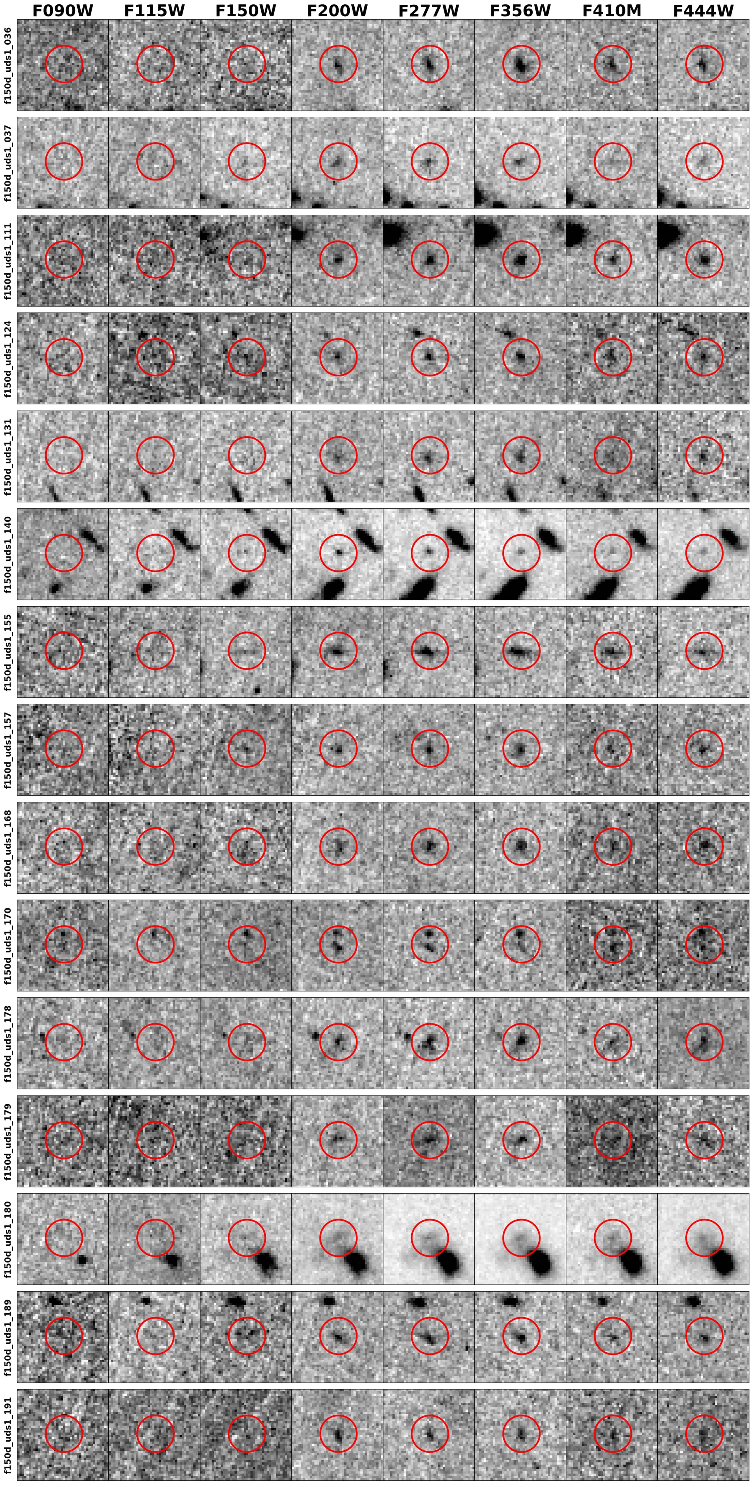
Figure A2: Similar to Figure 1; for the F150W dropouts in UDS1.

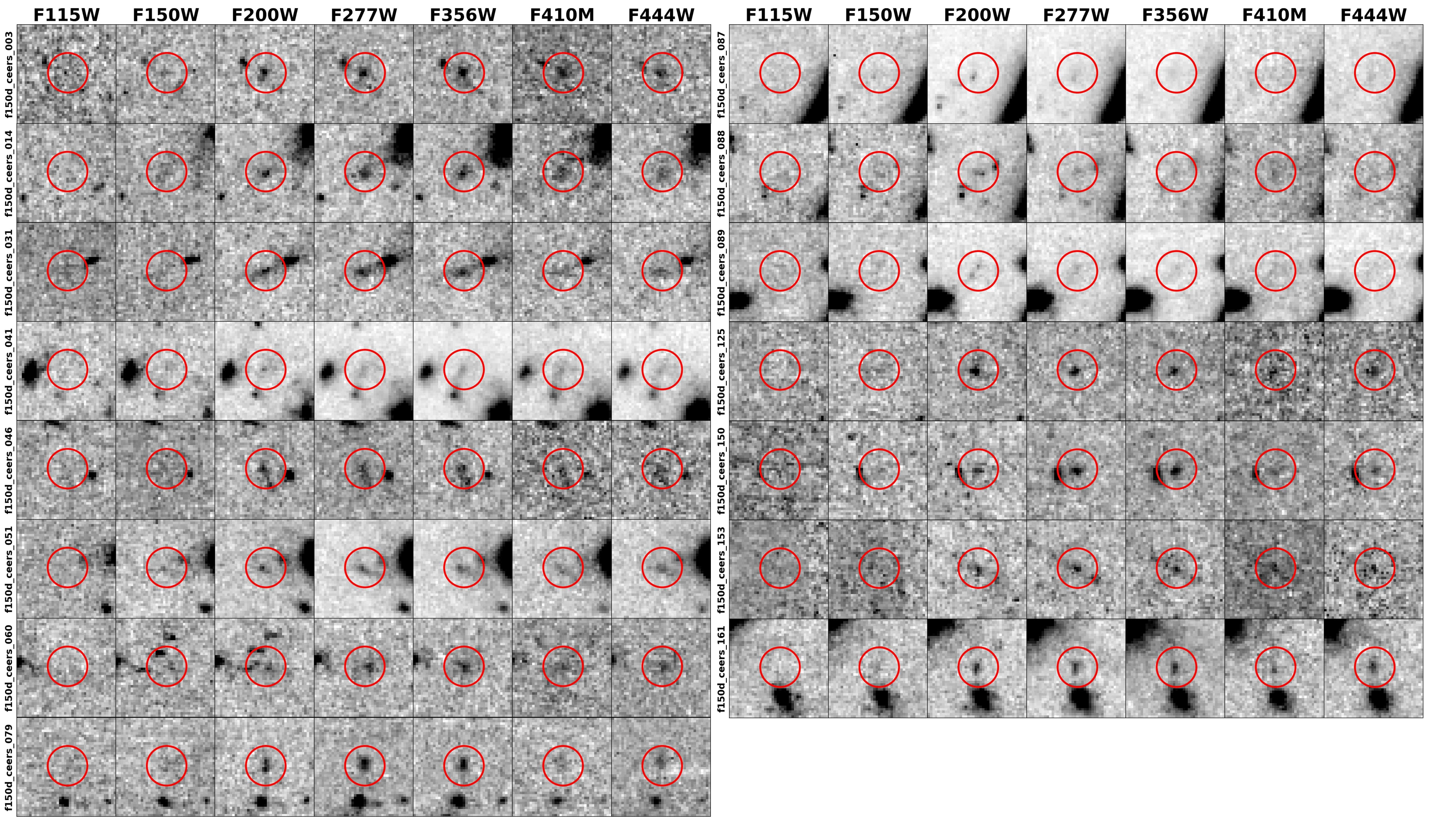
Figure A3: Similar to Figure 1; for the F150W dropouts in CEERS.

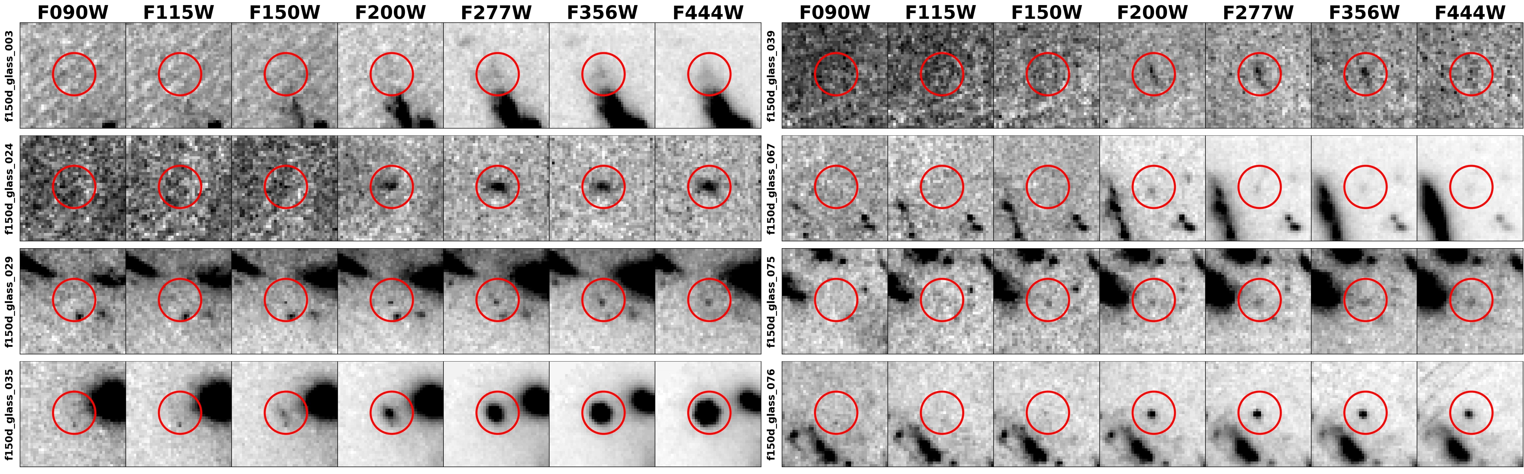
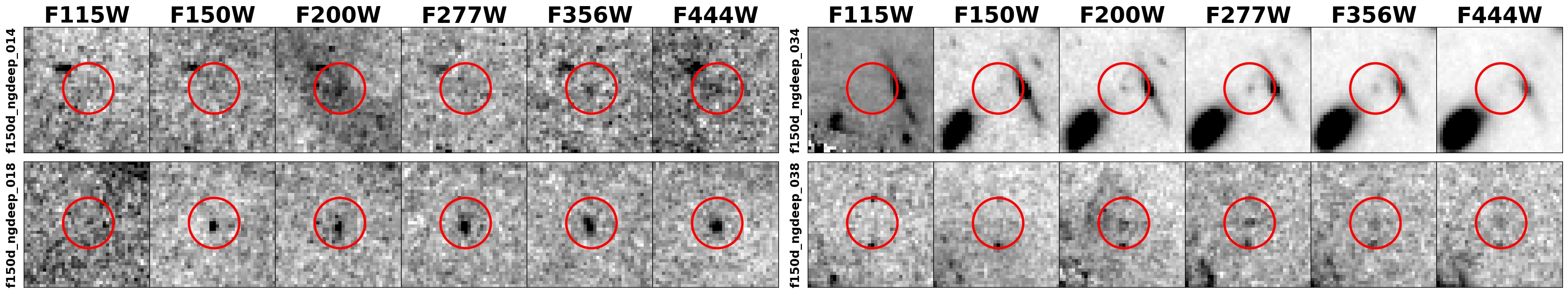
Figure A4: Similar to Figure 1; for the F150W dropouts in GLASS and NGDEEP

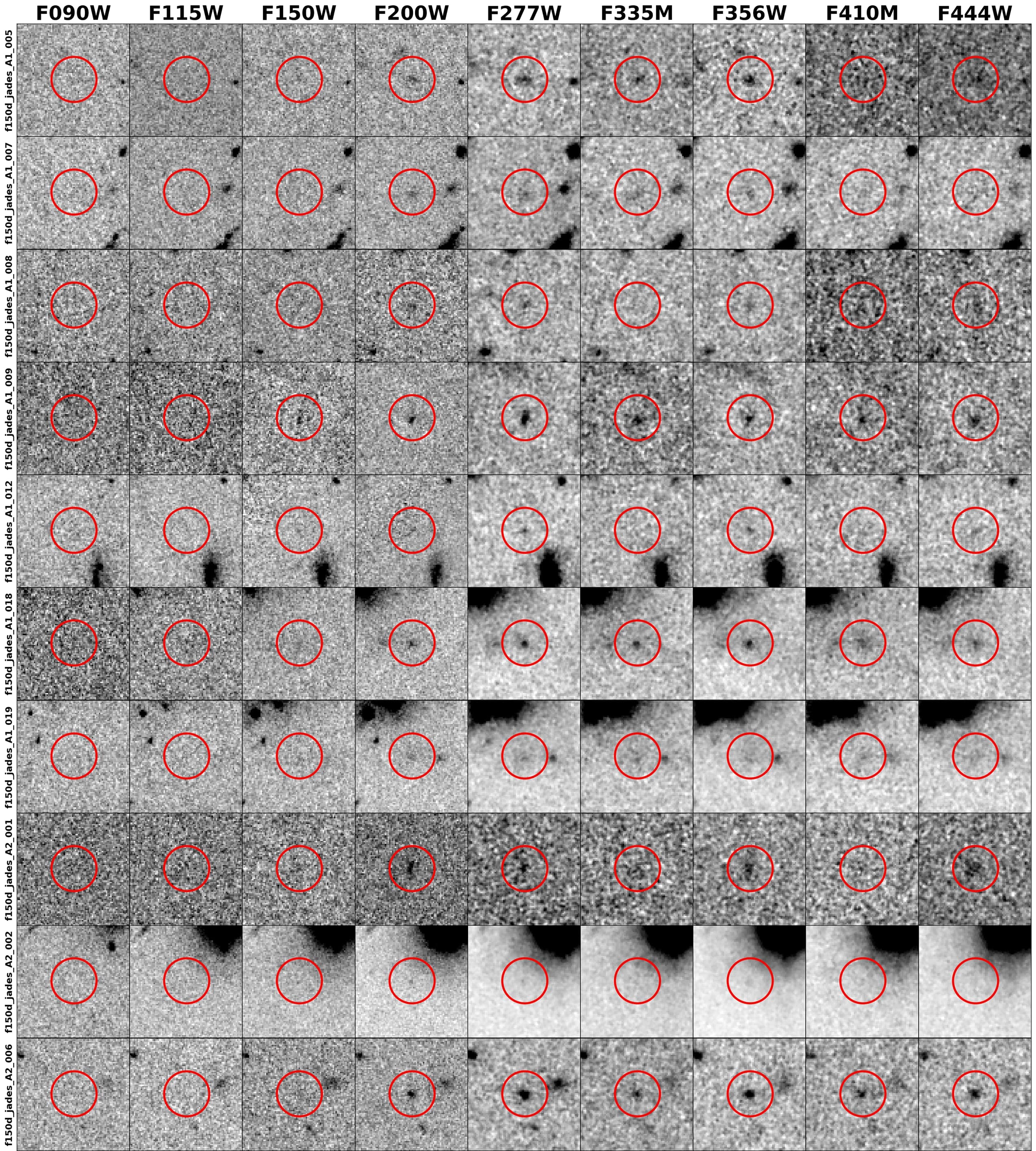
Figure A5: Similar to Figure 1; for the F150W dropouts in JADES GOODS-S.

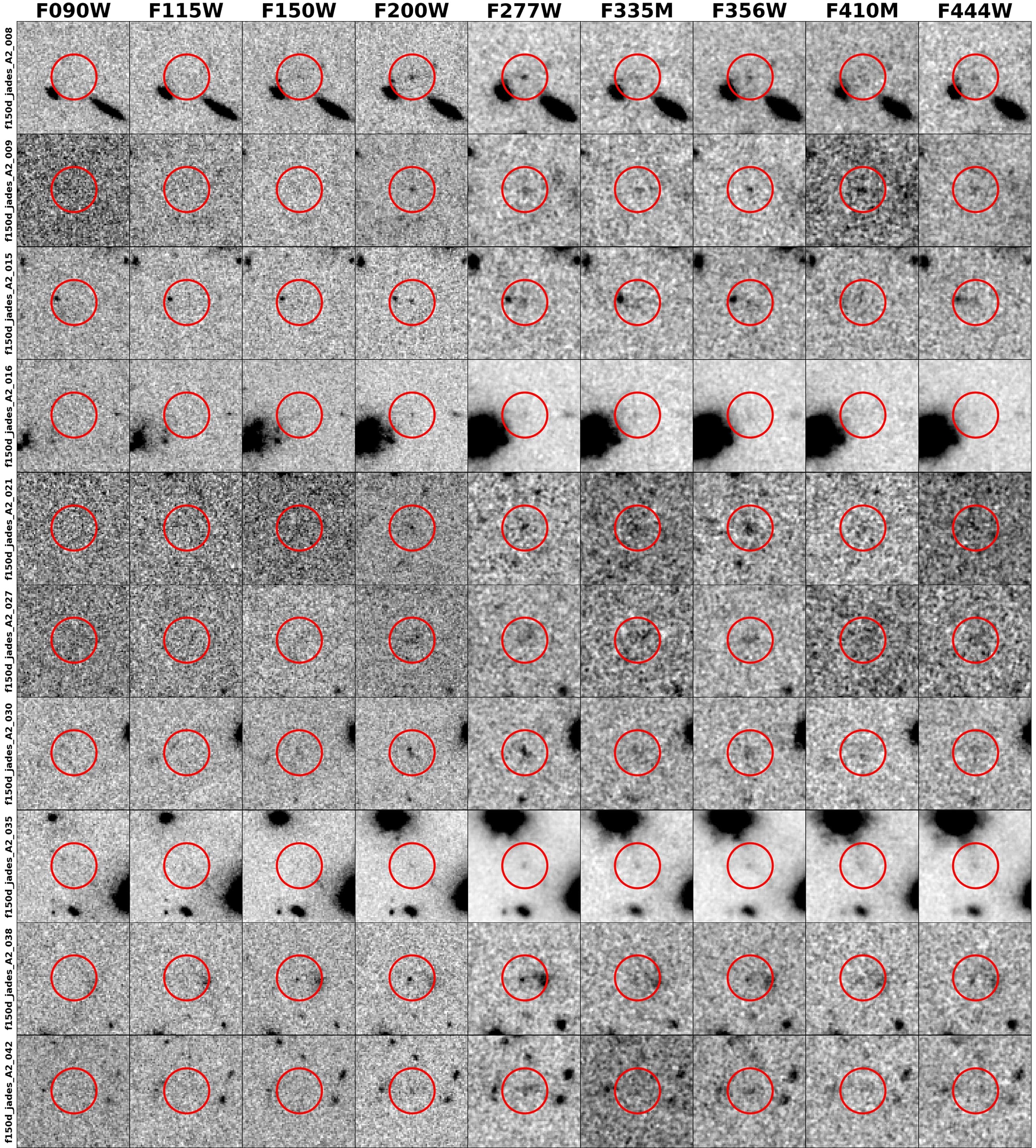
Figure A5 (Cont.): Similar to Figure 1; for the F150W dropouts in JADES GOODS-S.

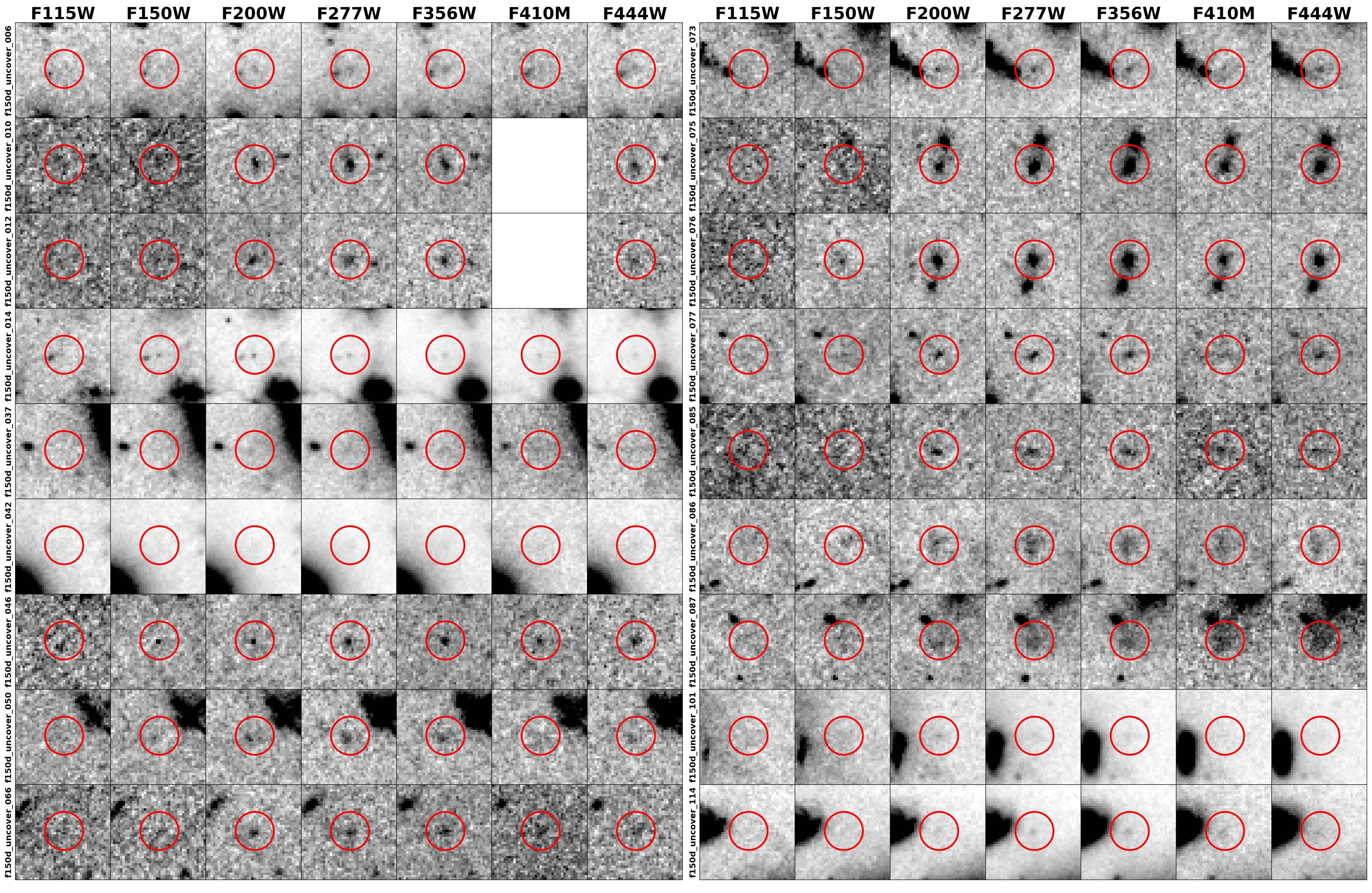
Figure A6: Similar to Figure 1; for the F150W dropouts in UNCOVER.

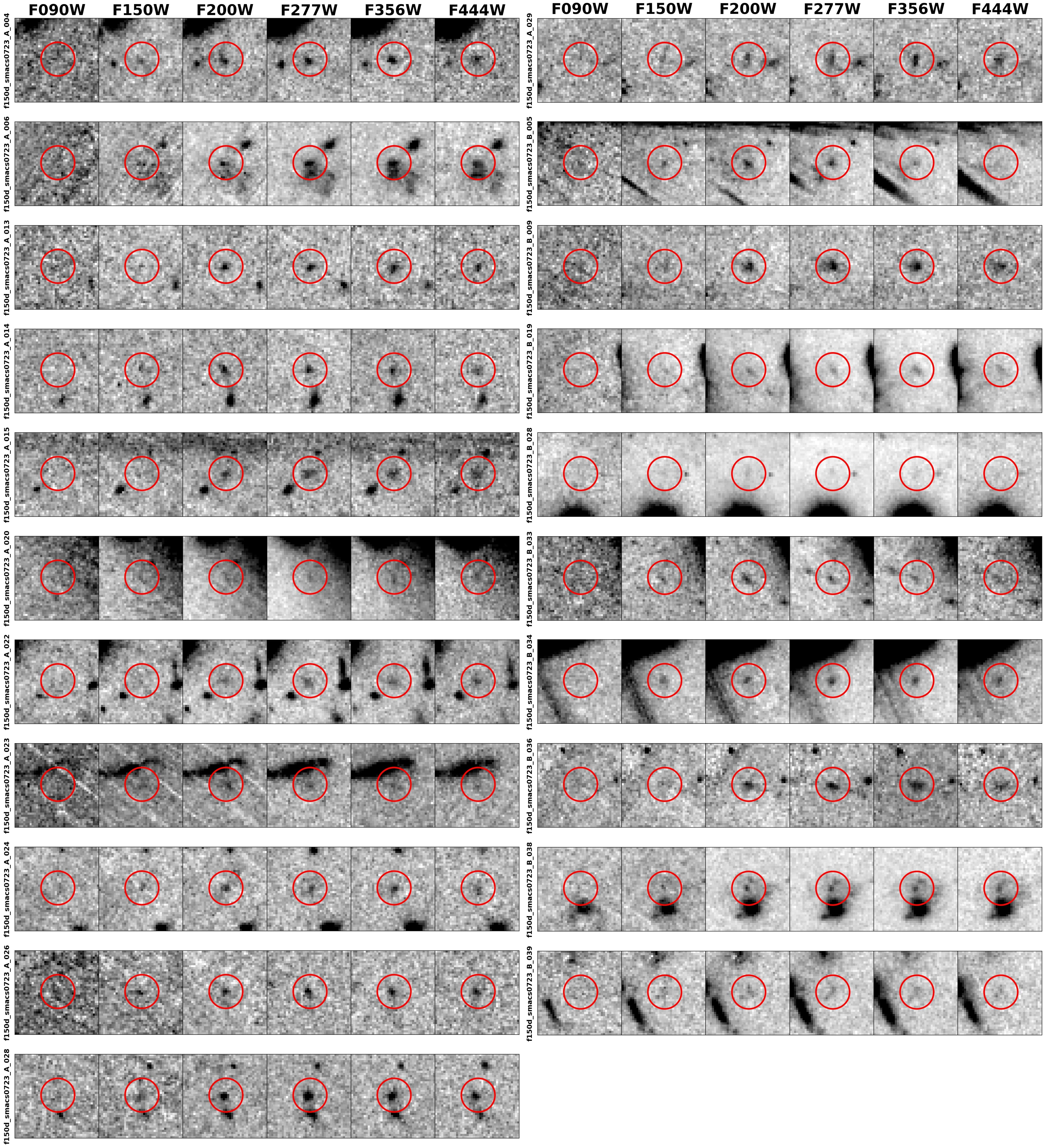
Figure A7: Similar to Figure 1; for the F150W dropouts in SMACS0723.

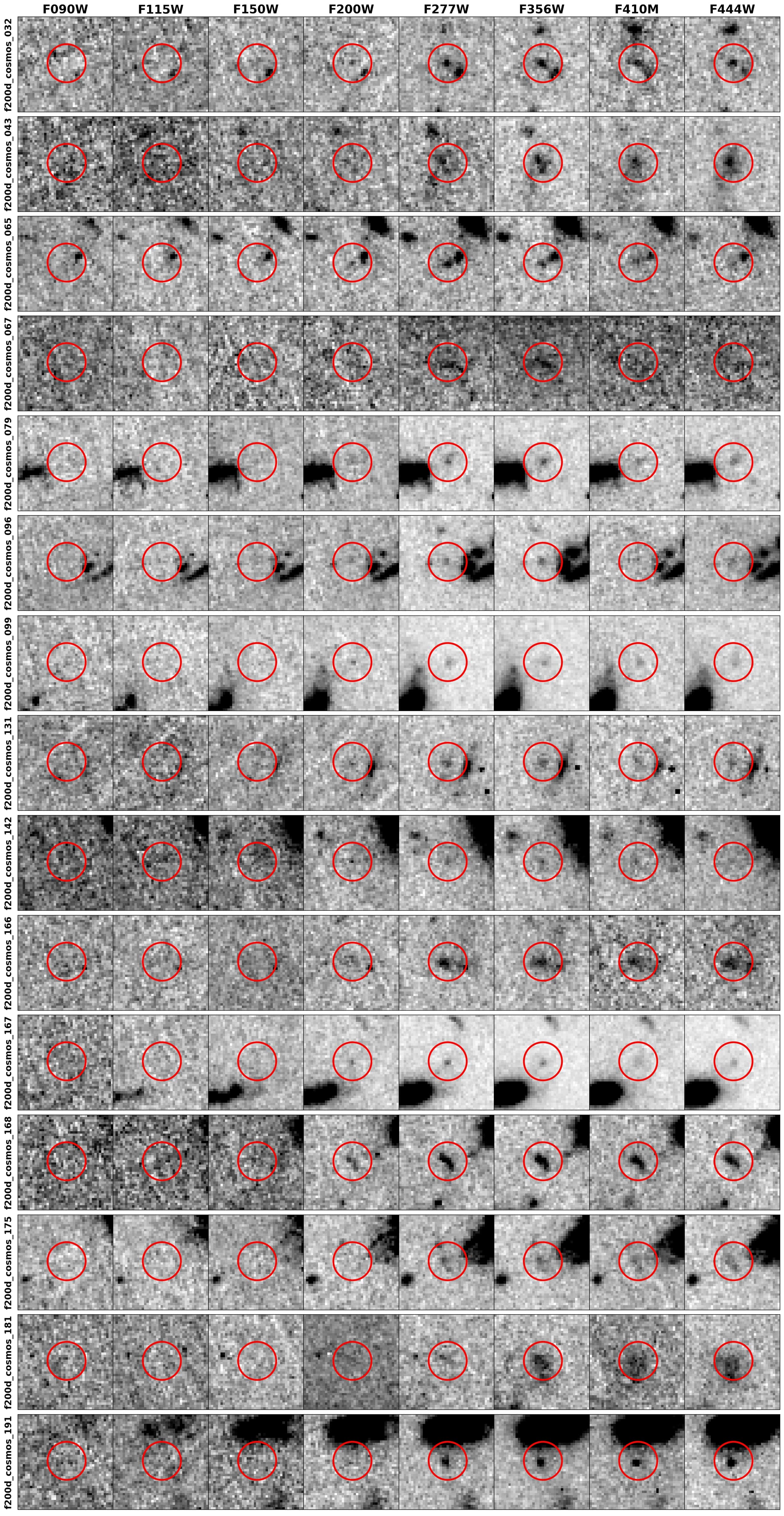
Figure A8: Similar to Figure 1; for the F200W dropouts in COSMOS.

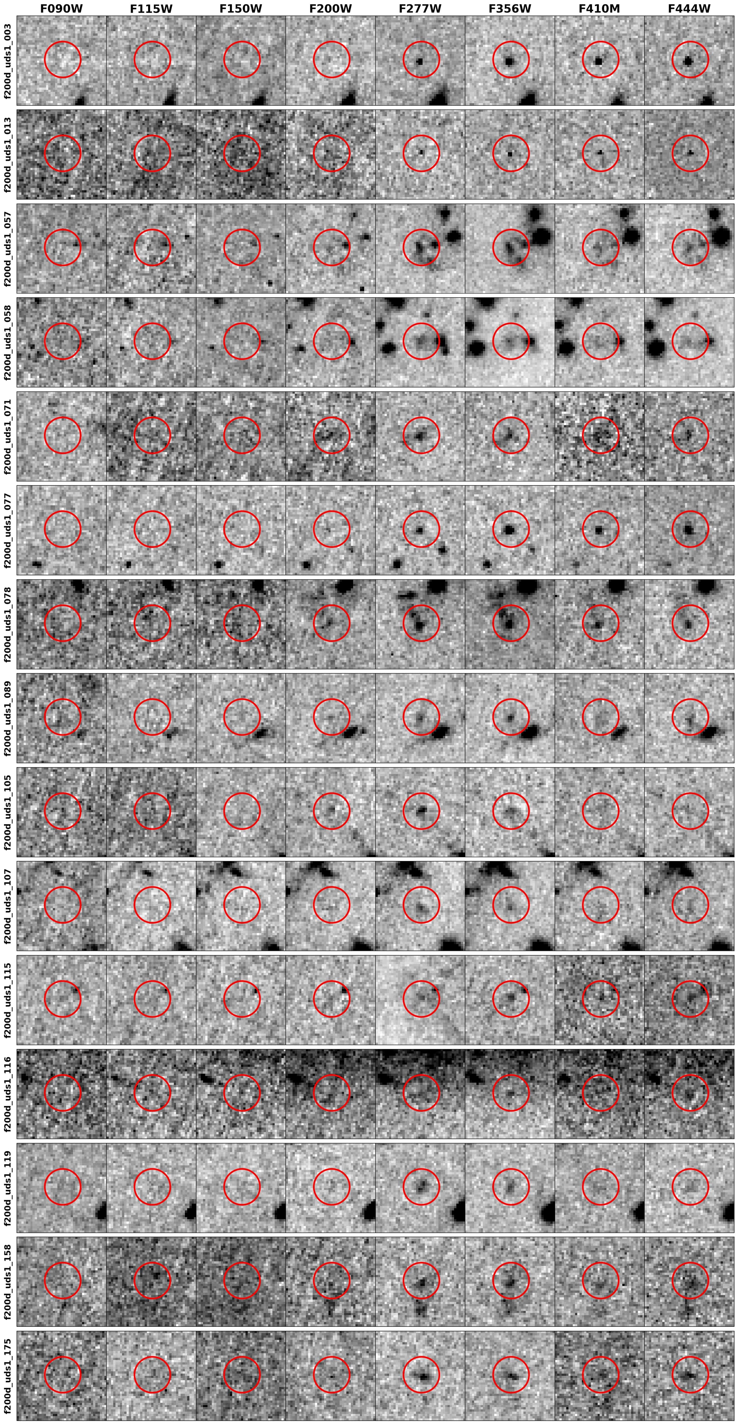
Figure A9: Similar to Figure 1; for the F200W dropouts in UDS1.

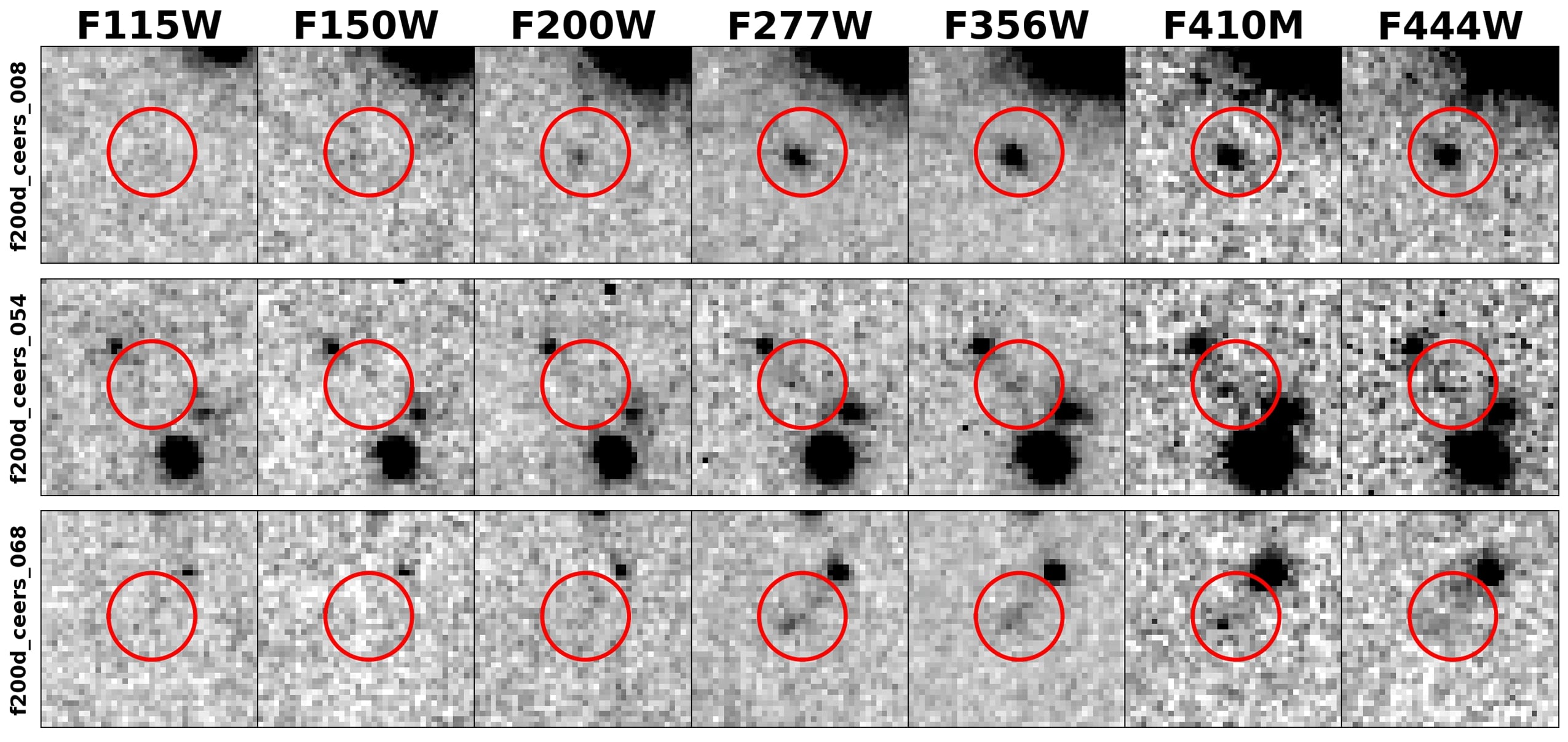
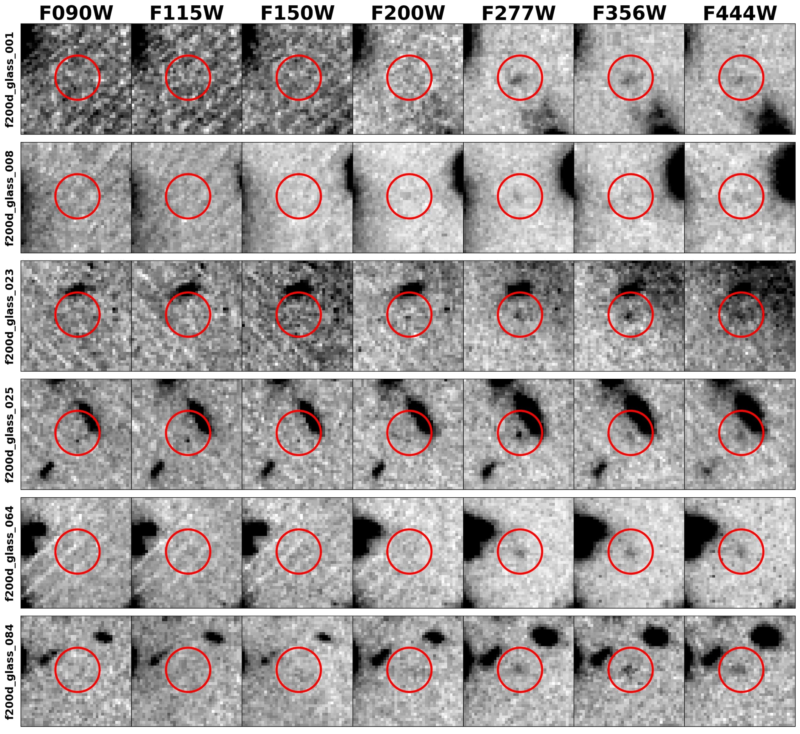
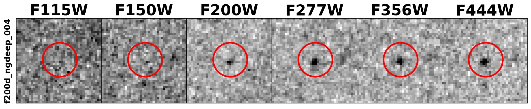
Figure A10: Similar to Figure 1; for the F200W dropouts in CEERS, GLASS and NGDEEP.

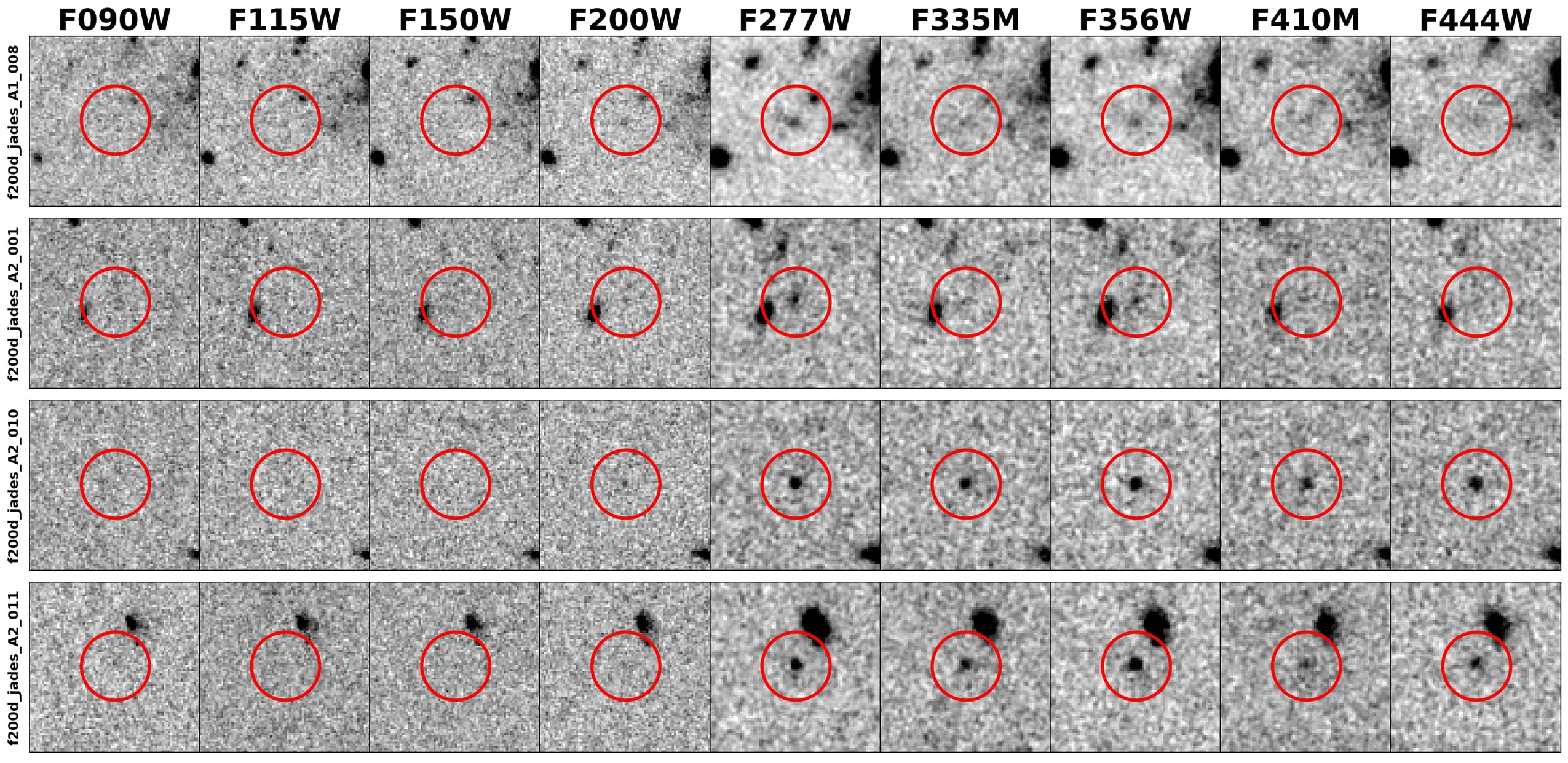
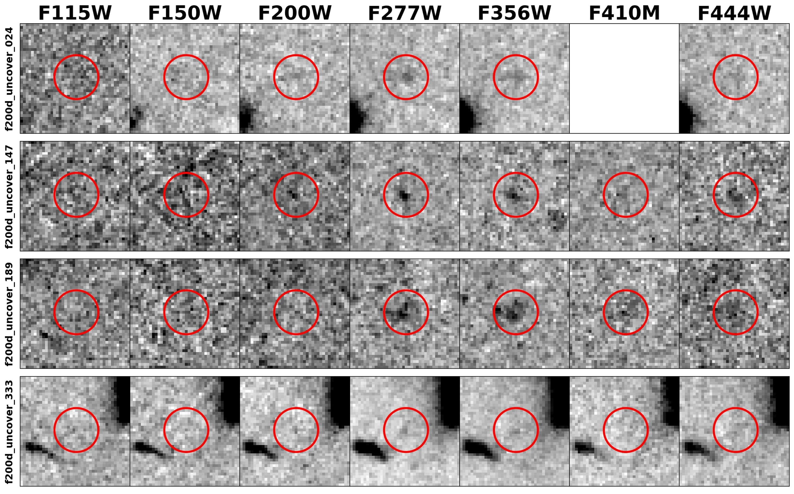
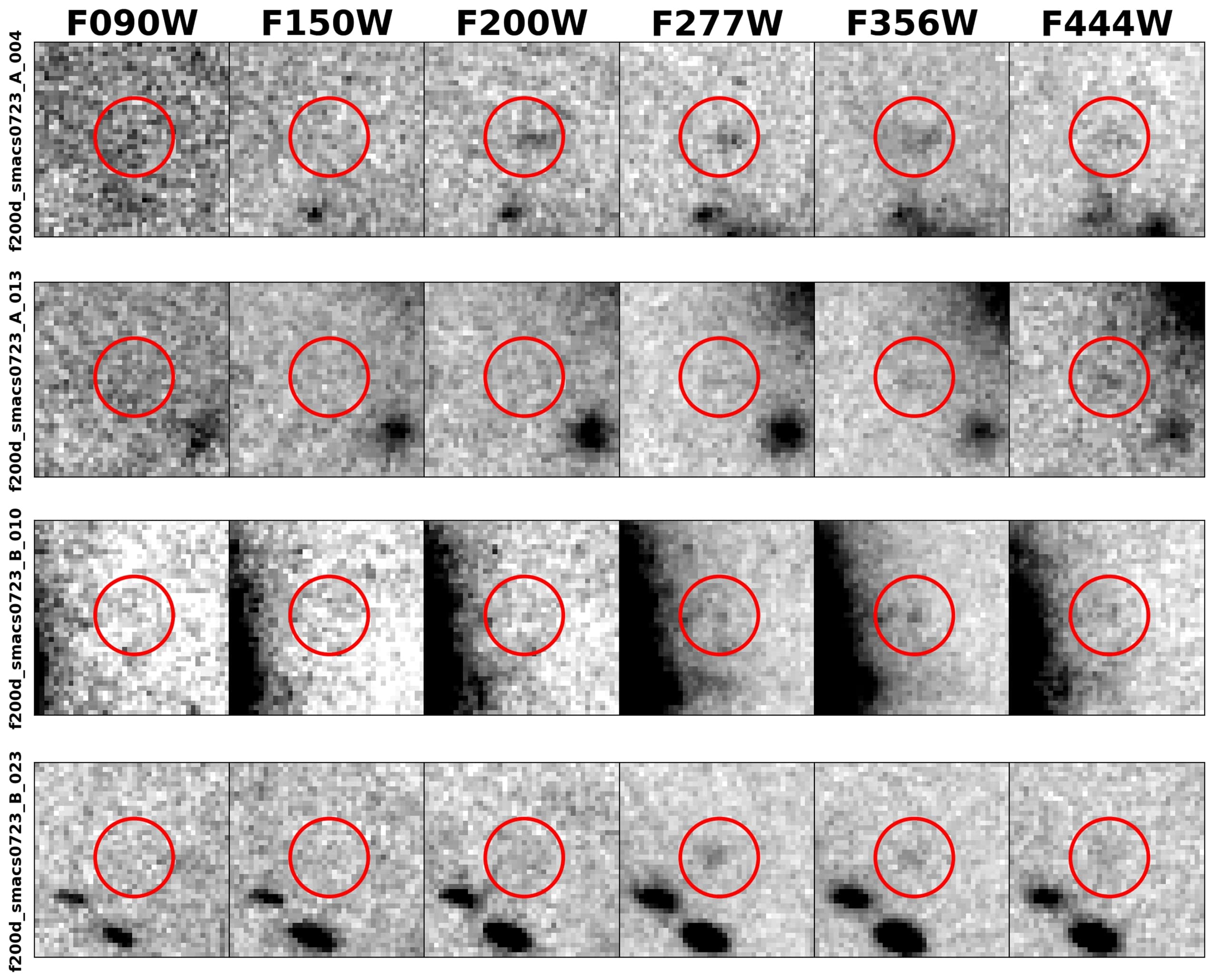
Figure A11: Similar to Figure 1; for the F200W dropouts in JADES GOODS-S, UNCOVER and SMACS0723.

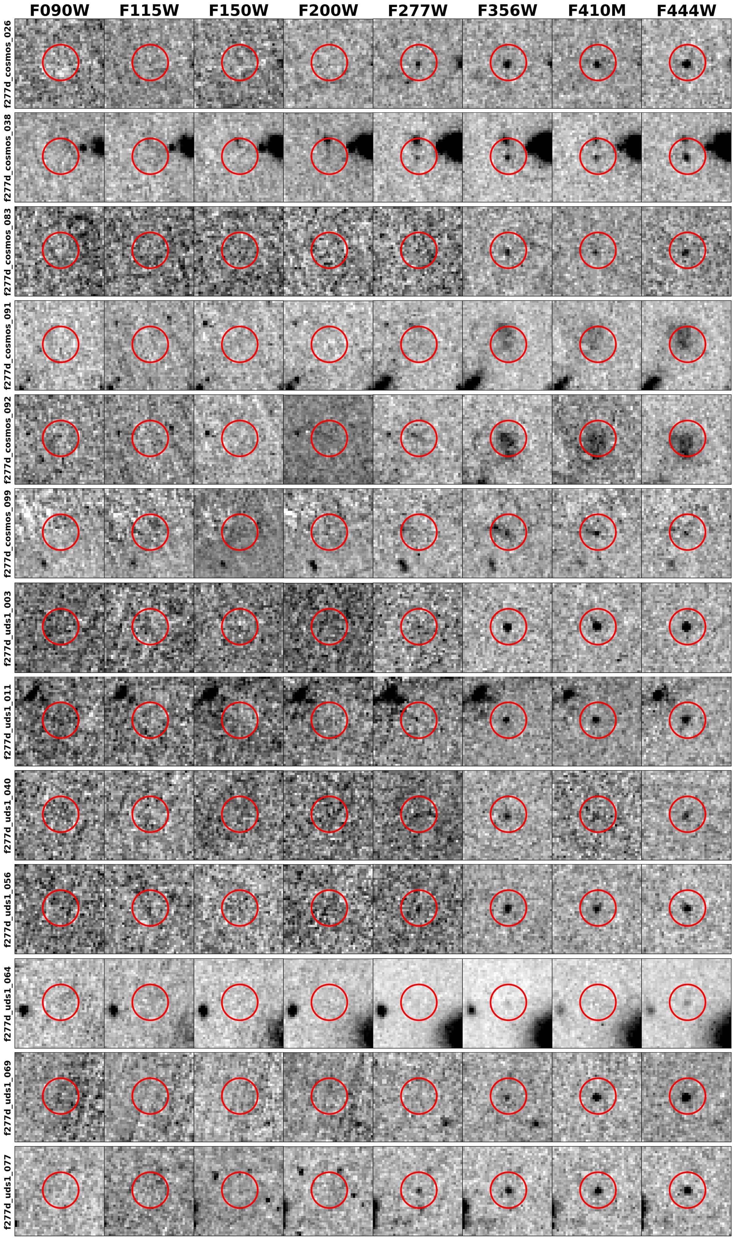
Figure A12: Similar to Figure 1; for the F277W dropouts in COSMOS and UDS1.

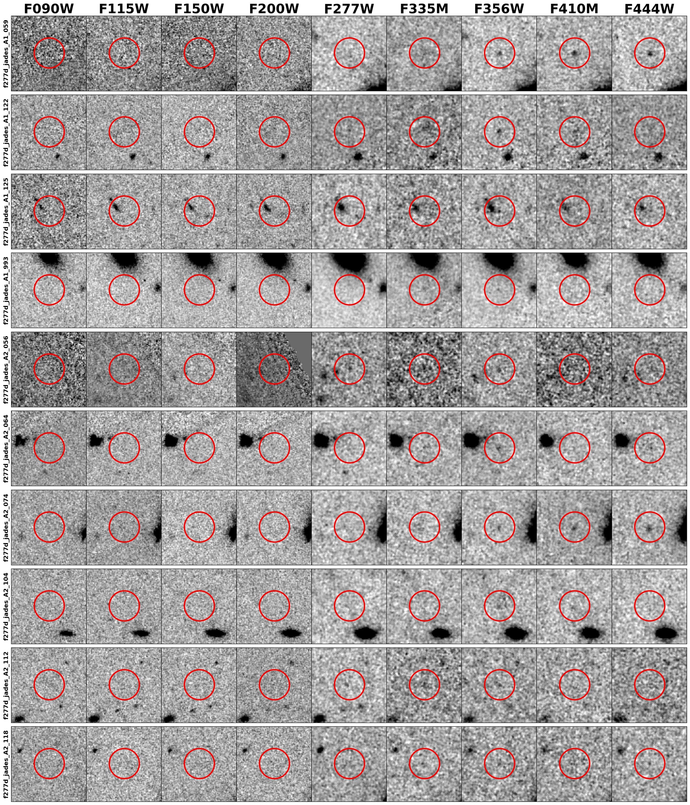
Figure A13: Similar to Figure 1; for the F277W dropouts in JADES GOODS-S.

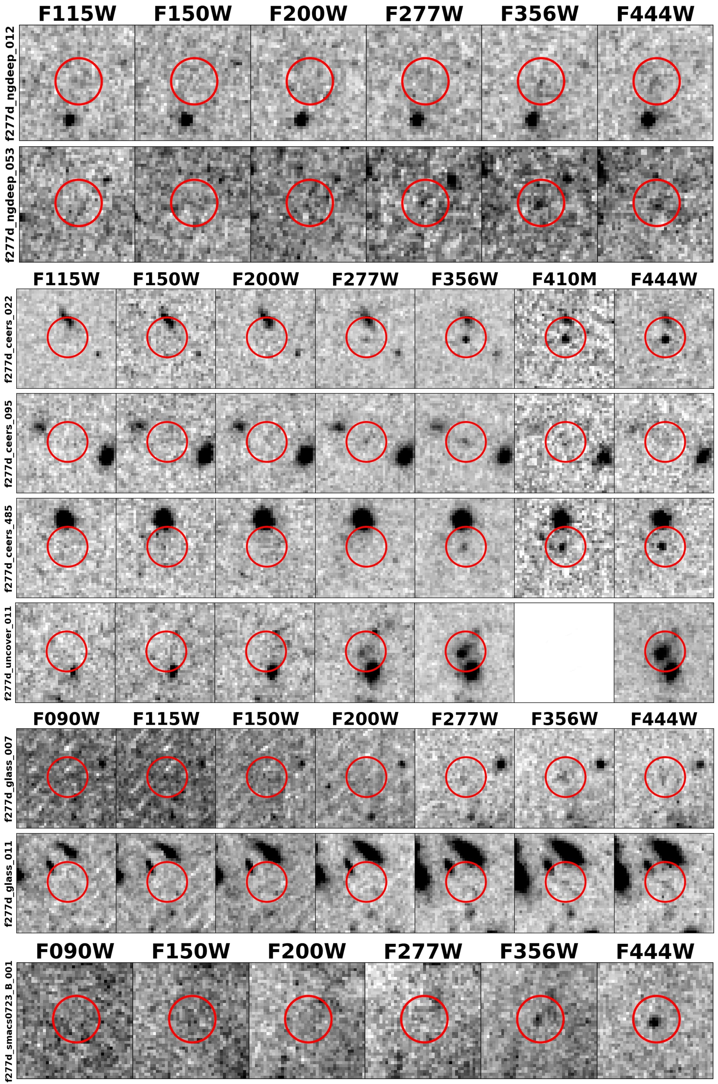
Figure A14: Similar to Figure 1; for the F277W dropouts in NGDEEP, CEERS, UNCOVER, GLASS, and SMACS0723.

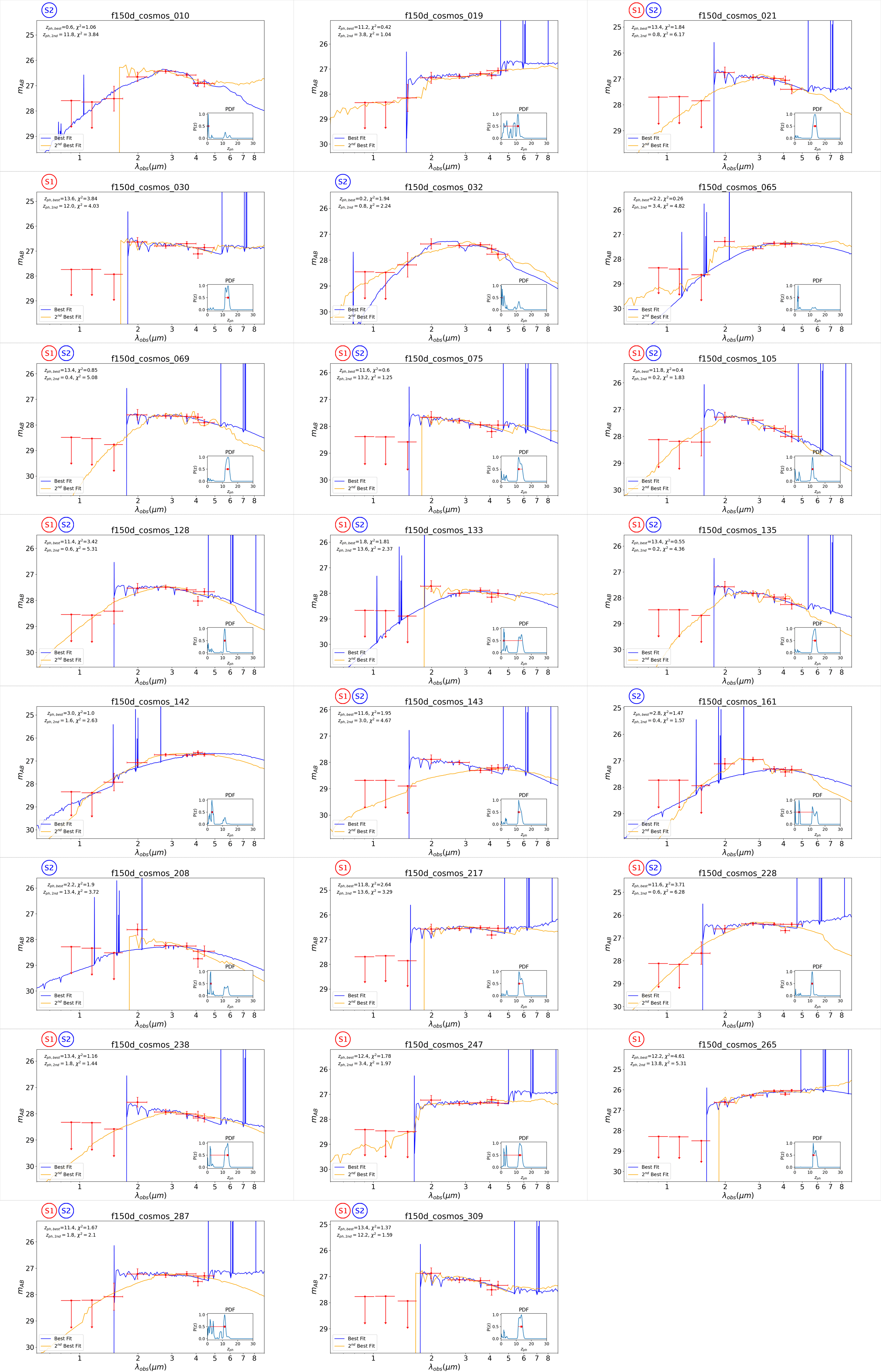
Figure A16: Same as Figure A15; for the F150W dropouts in COSMOS.

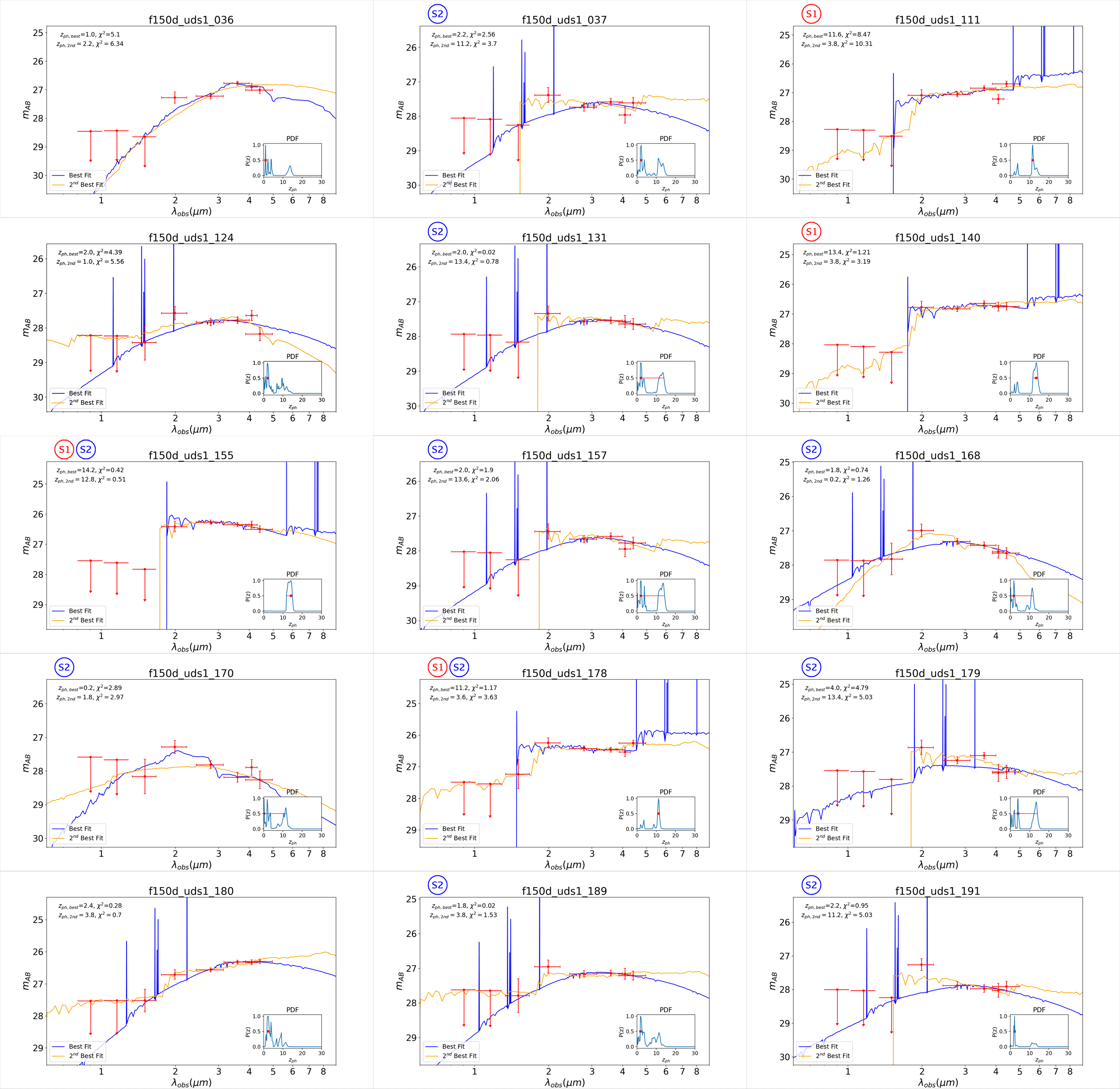
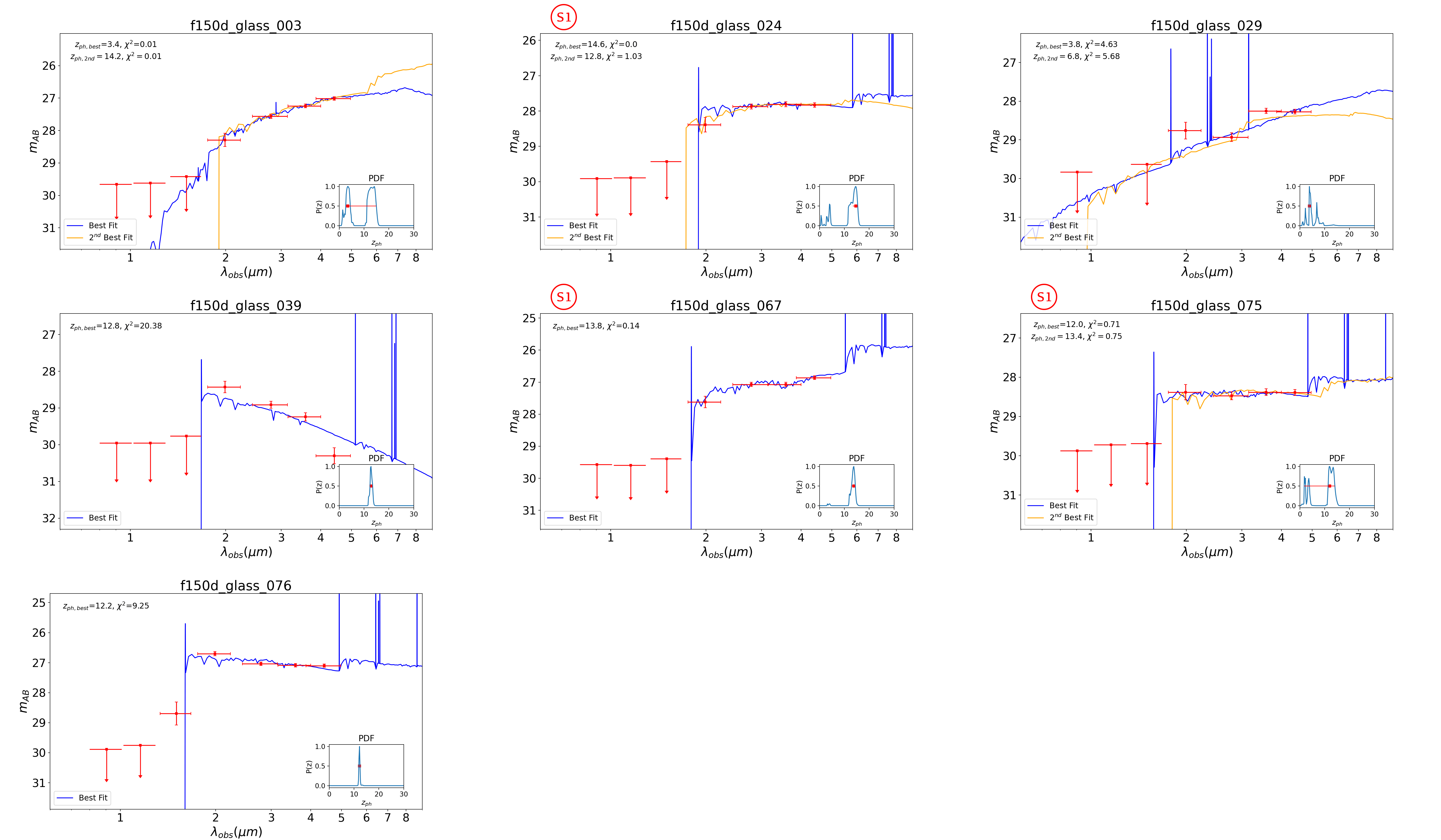
Figure A17: Same as Figure A15; for the F150W dropouts in UDS1 and GLASS.

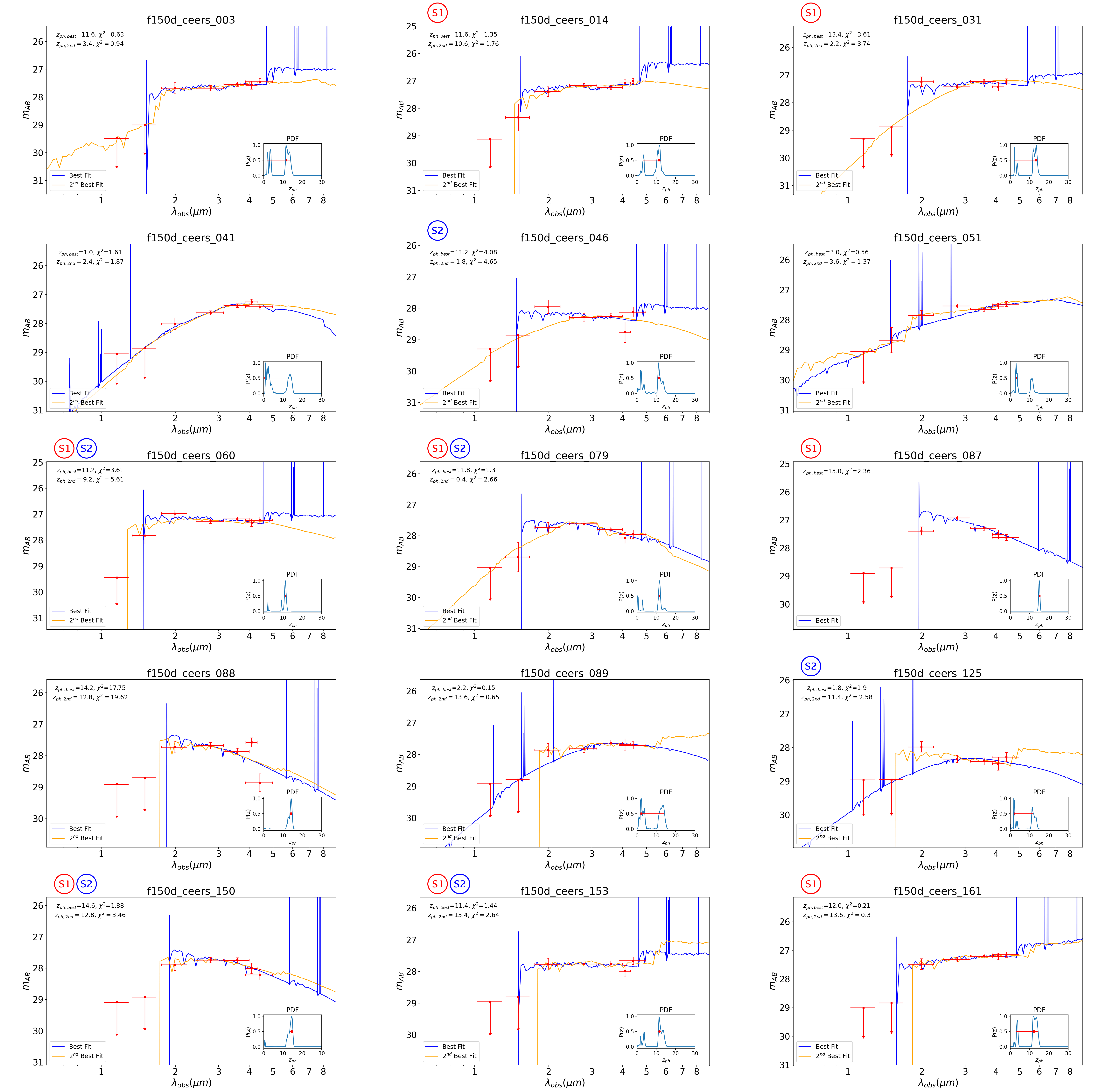
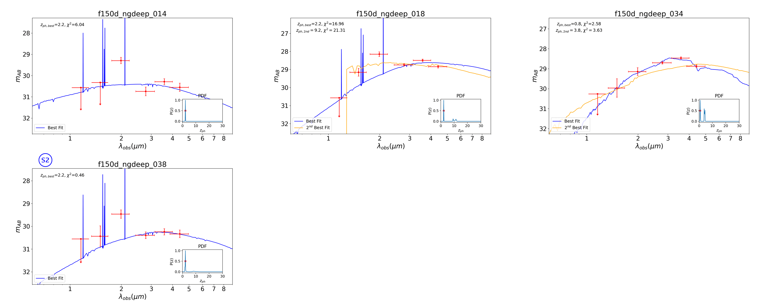
Figure A18: Same as Figure A15; for the F150W dropouts in CEERS and NGDEEP.

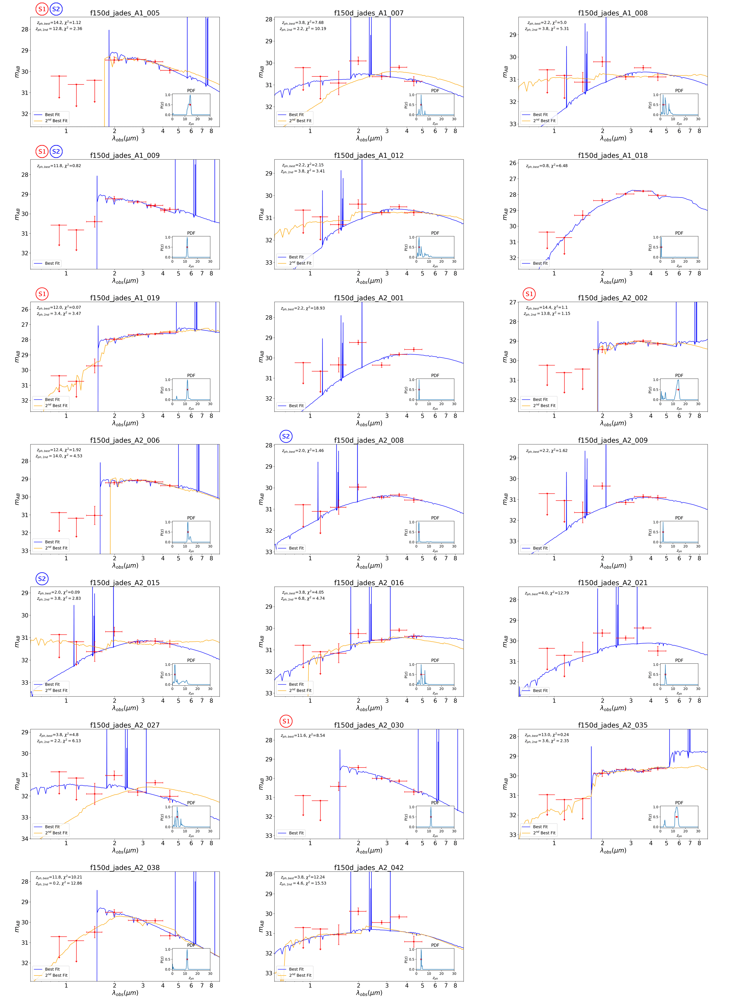
Figure A19: Same as Figure A15; for the F150W dropouts in JADES GOODS-S.

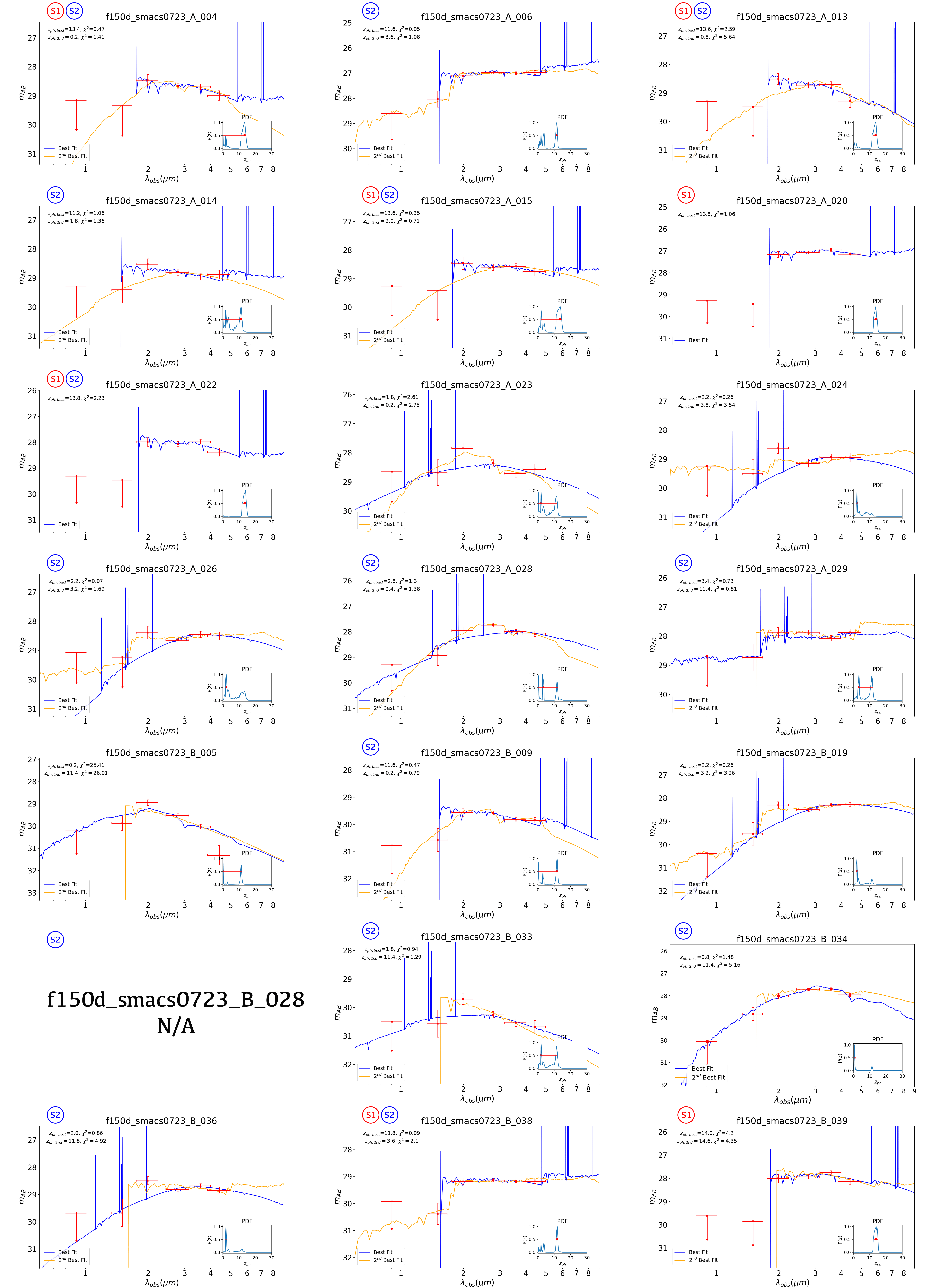
Figure A20: Same as Figure A15; for the F150W dropouts in SMACS0723. The fitting fails for f150d_smacs0723_B_028, which is not shown.

Figure A21: Scheme 2 (S2; using EAZY and the “set 3+4” templates ) SED fitting results for F150W dropouts in UNCOVER. Each panel shows one F150W dropout, whose SID is labeled to left. The PDF is shown in the smaller panel to right. The dark blue curve is the spectrum of the best-fit model corresponding to the first peak of the PDF, which also gives $z_{\rm ph}$ as labeled. If an object is retained in S1 and/or S2, the plot is marked with {\tinyS1}⃝ and/or {\tinyS2}⃝.

Figure A22: Same as Figure A21; for the F150W dropouts in COSMOS.

Figure A23: Same as Figure A21; for the F150W dropouts in UDS1 and GLASS.

Figure A24: Same as Figure A21; for the F150W dropouts in CEERS and NGDEEP.

Figure A25: Same as Figure A21; for the F150W dropouts in JADES GOODS-S.

Figure A26: Same as Figure A21; for the F150W dropouts in SMACS0723.

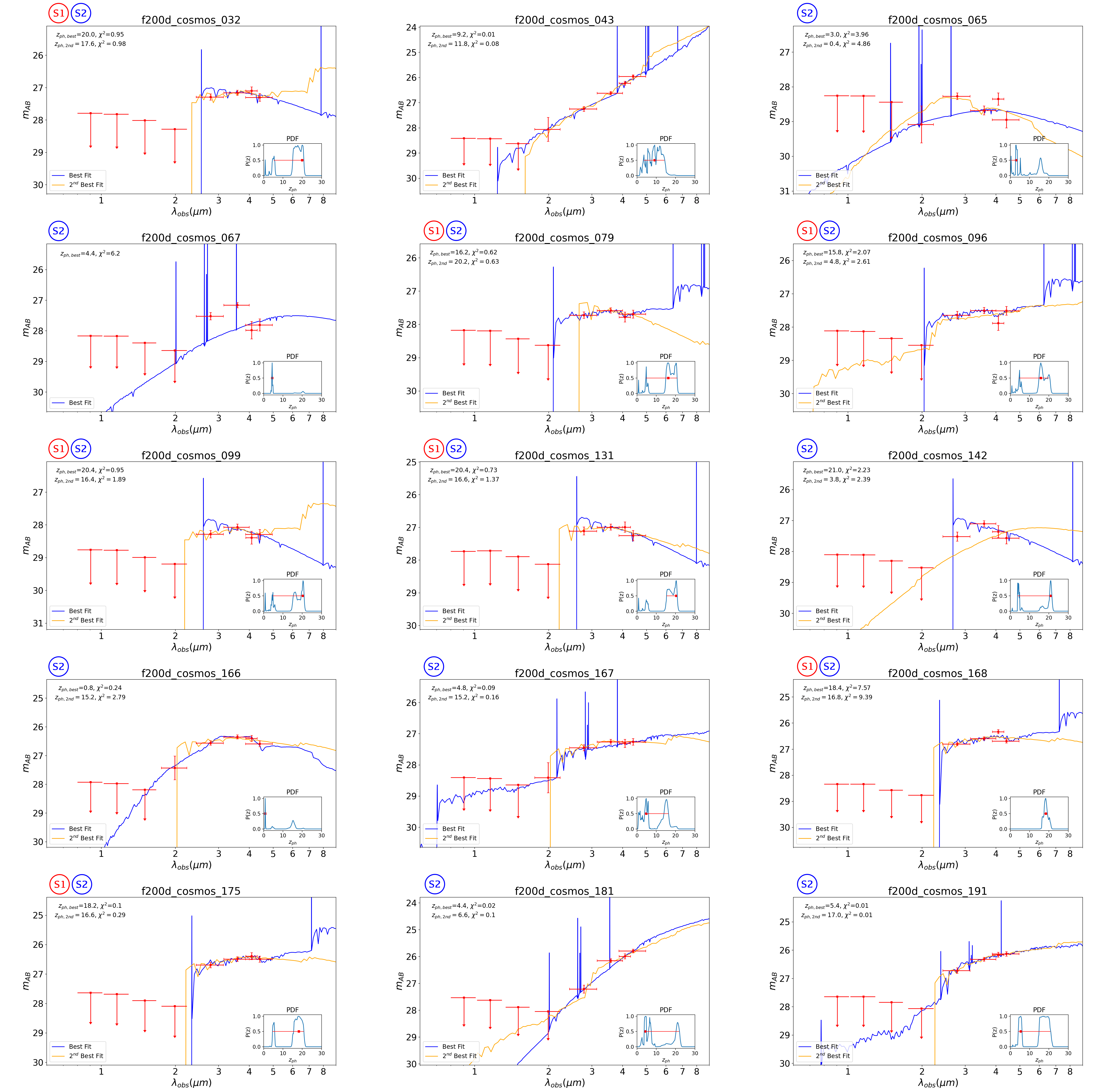
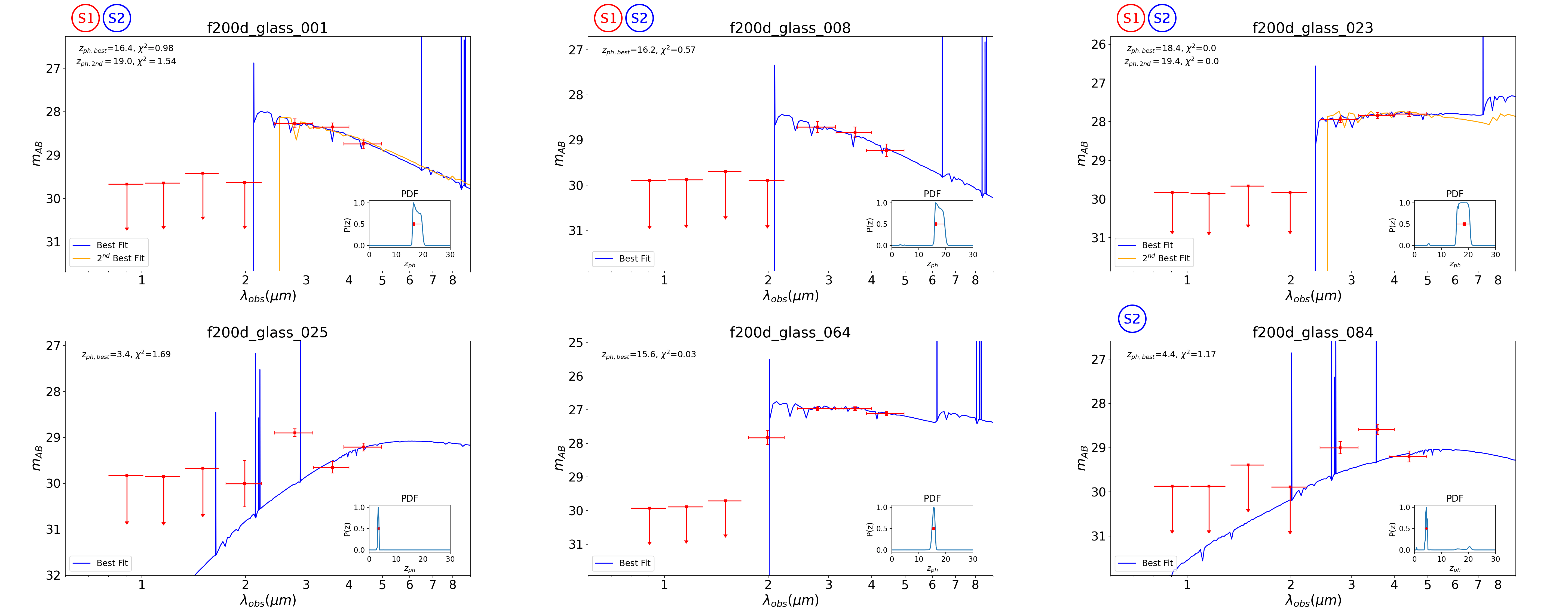
Figure A27: Same as Figure A15; for the F200W dropouts in COSMOS and GLASS.

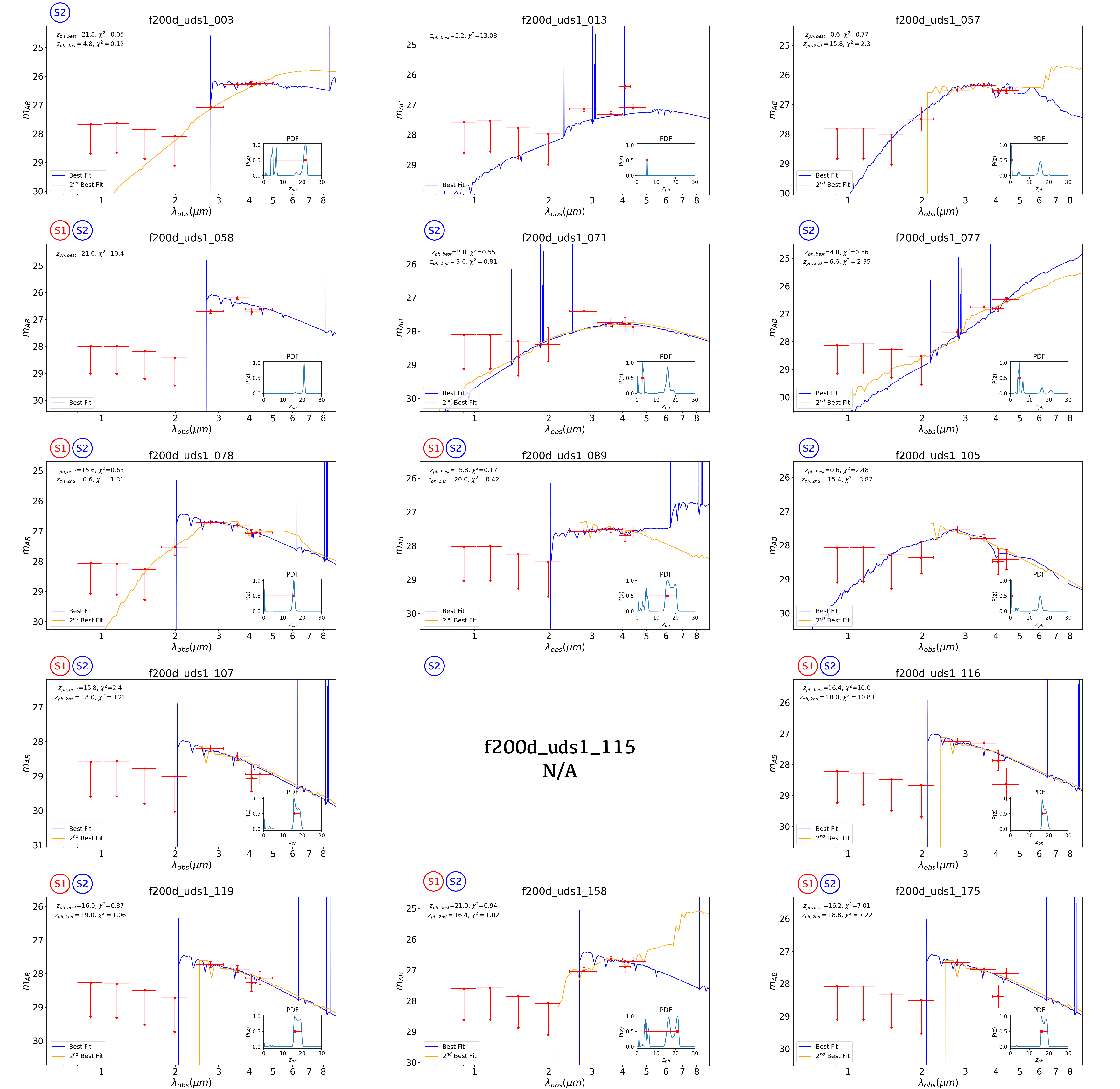
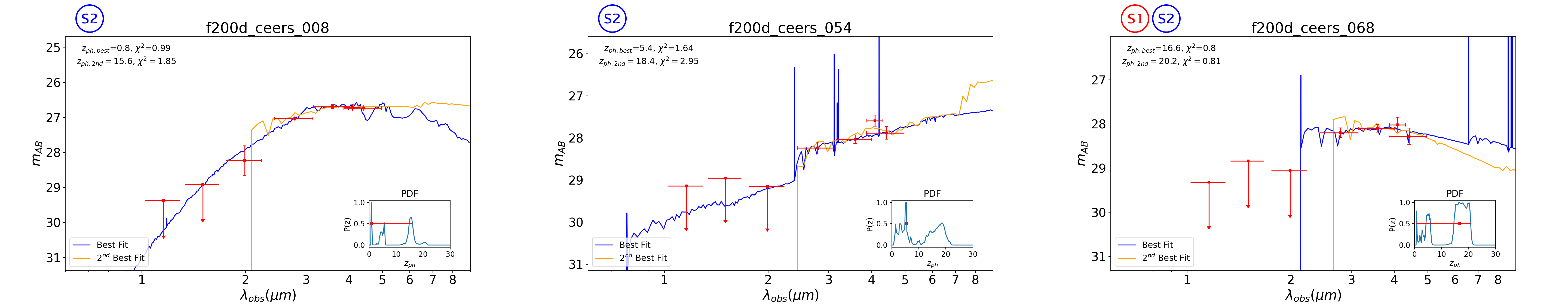
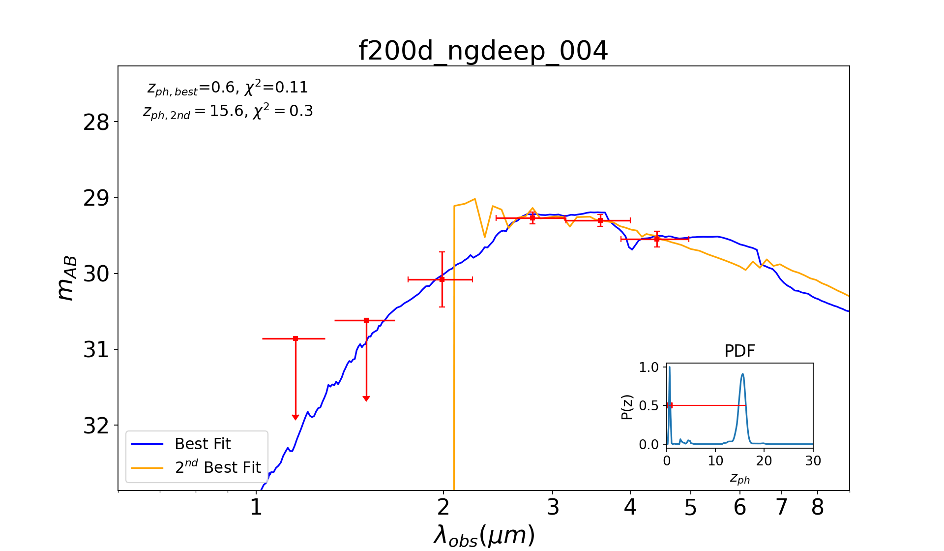
Figure A28: Same as Figure A15; for the F200W dropouts in UDS1 (f200d_uds1_115 not included due to the failed fit), CEERS and NGDEEP.

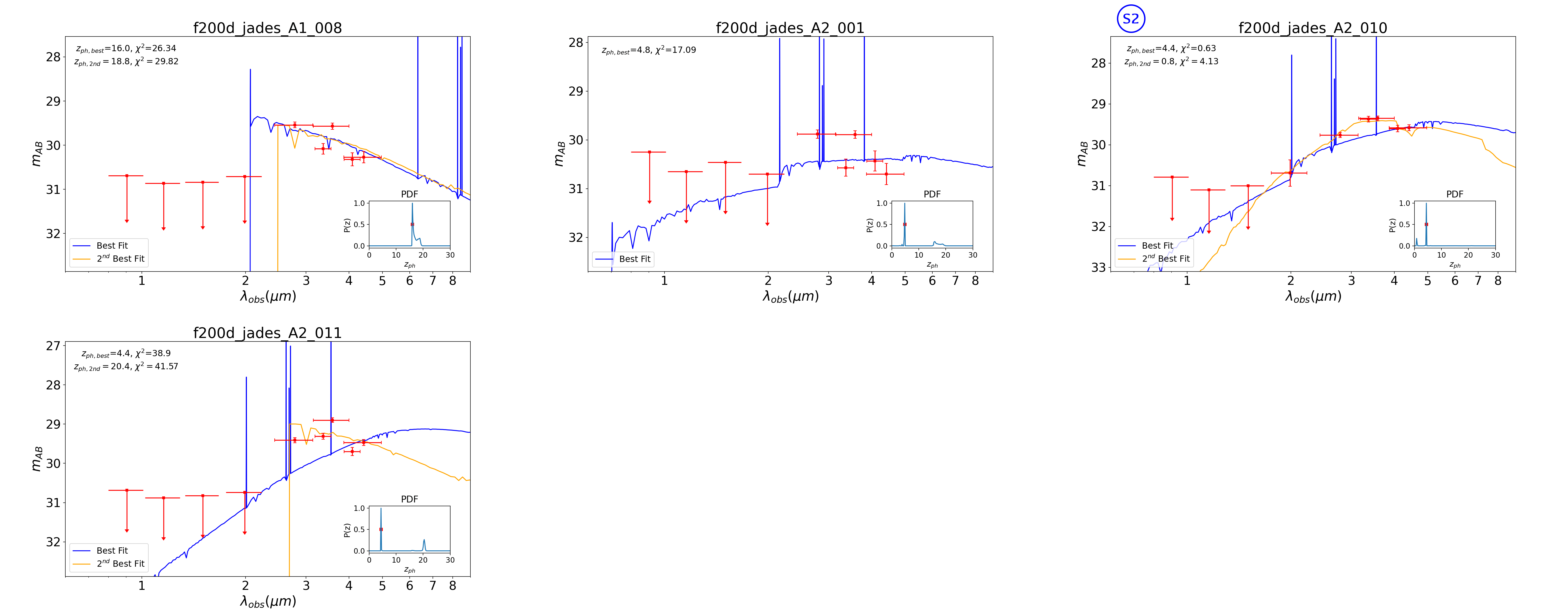
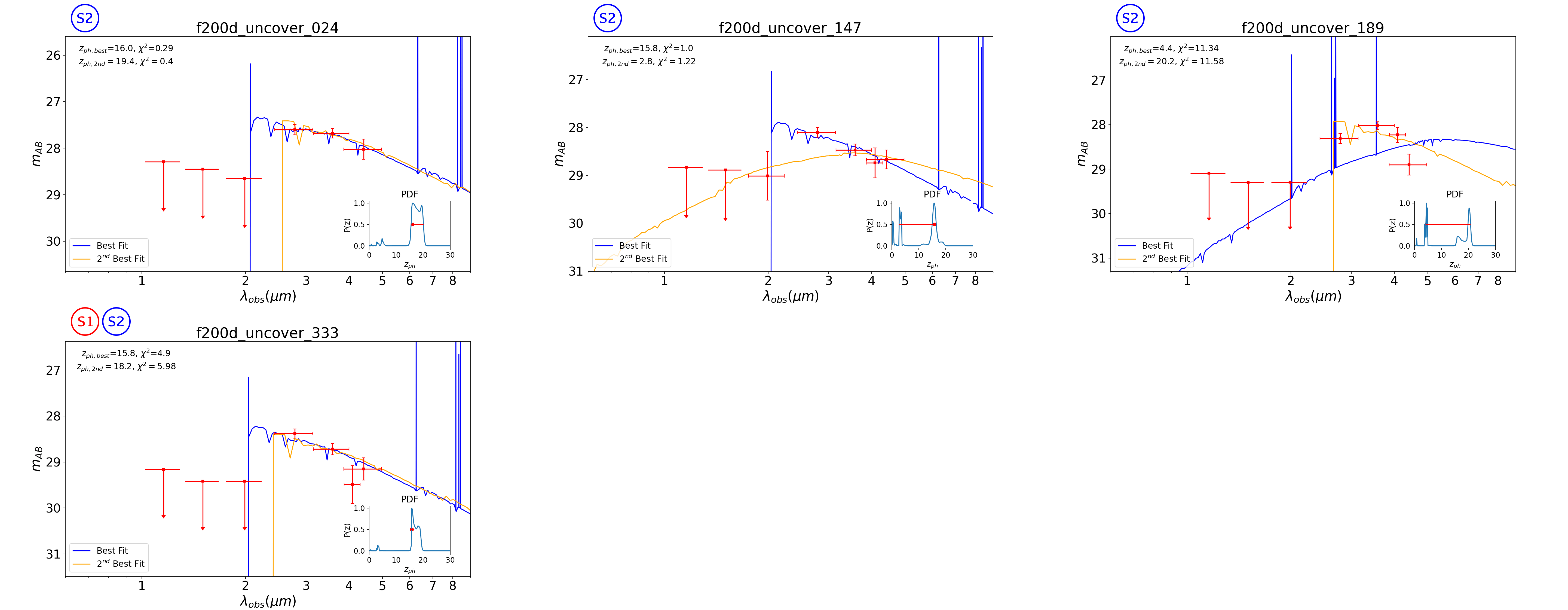
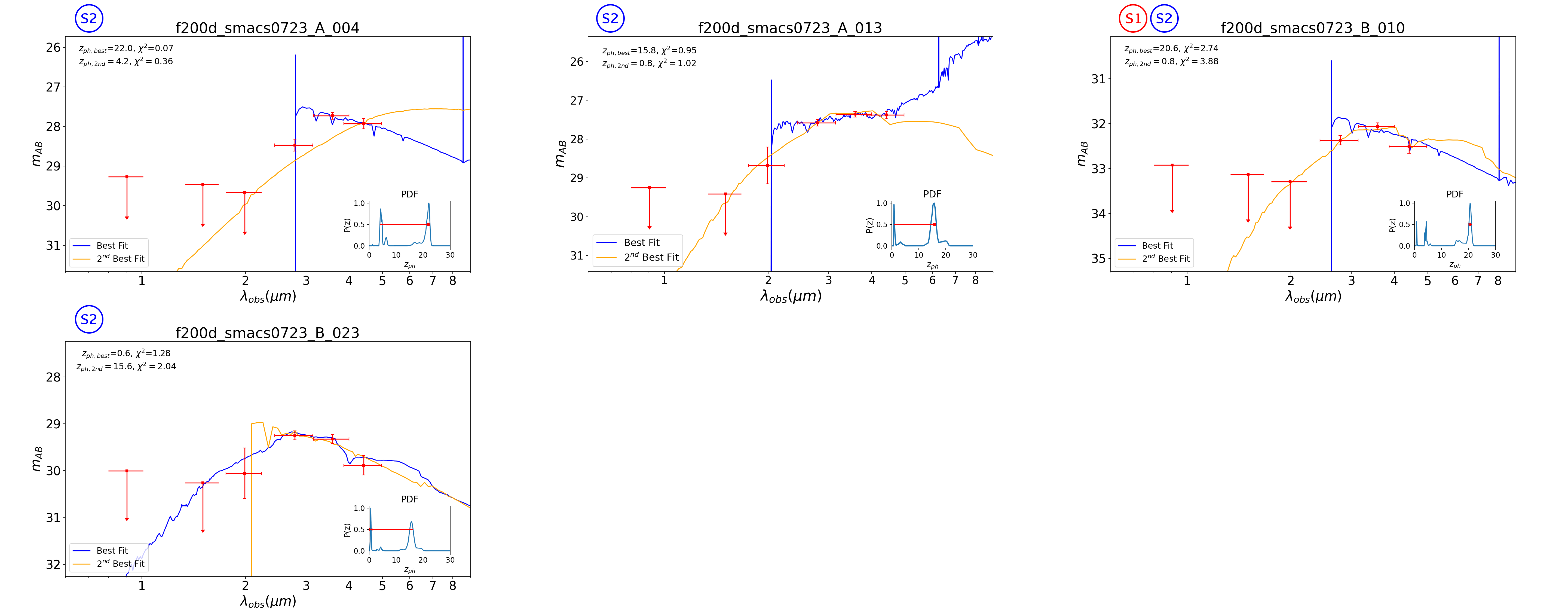
Figure A29: Same as Figure A15; for the F200W dropouts in JADES GOODS-S, UNCOVER and SMACS0723.

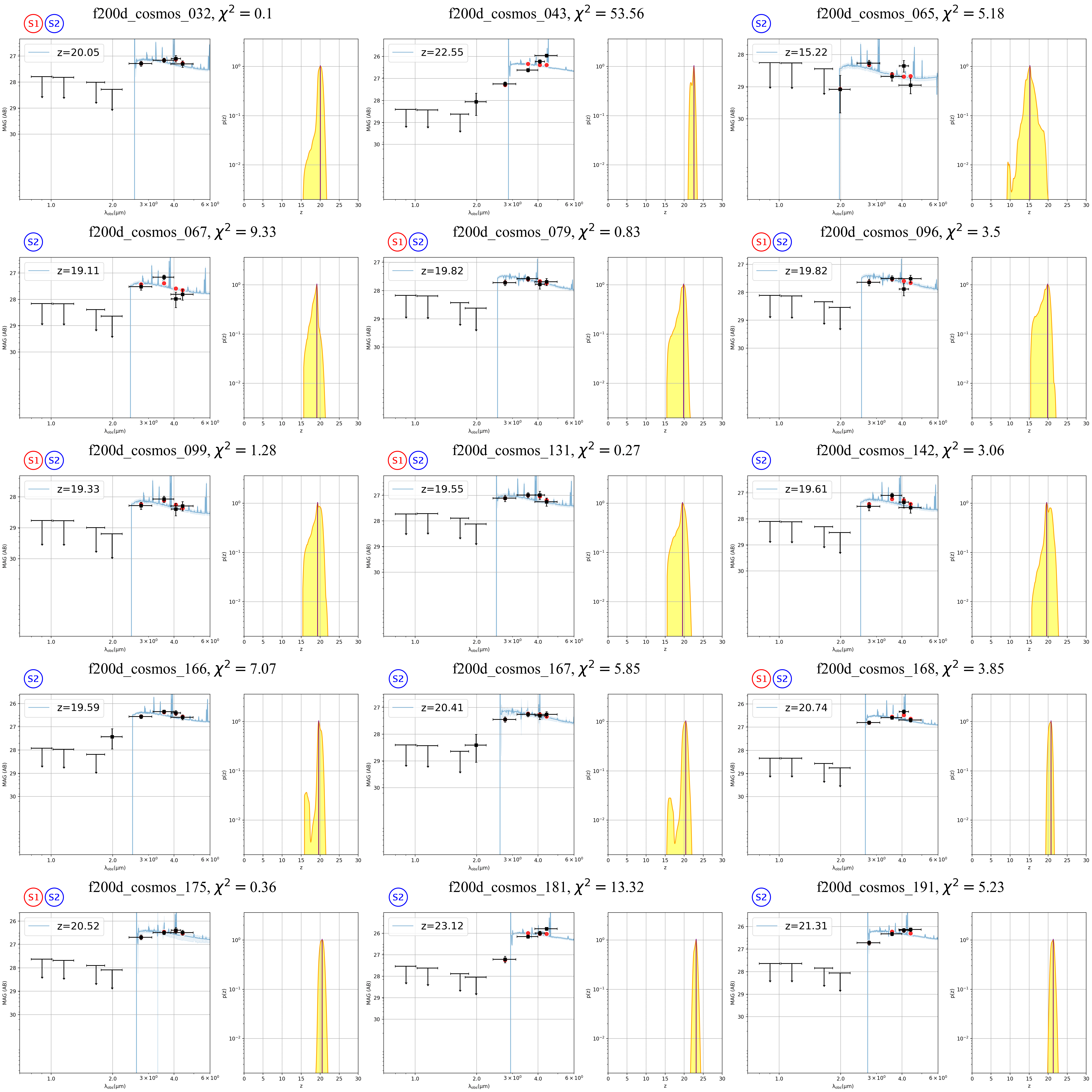
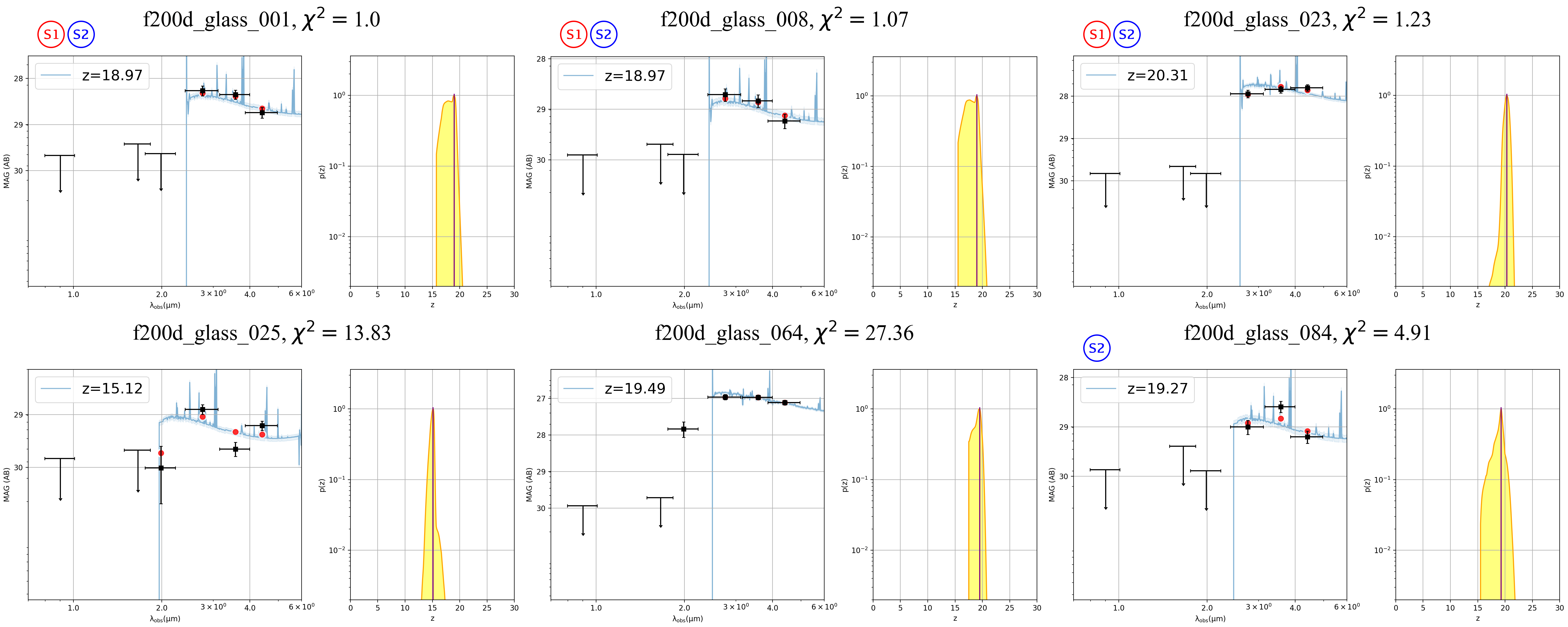
Figure A30: Same as Figure A21; for the F200W dropouts in COSMOS and GLASS.

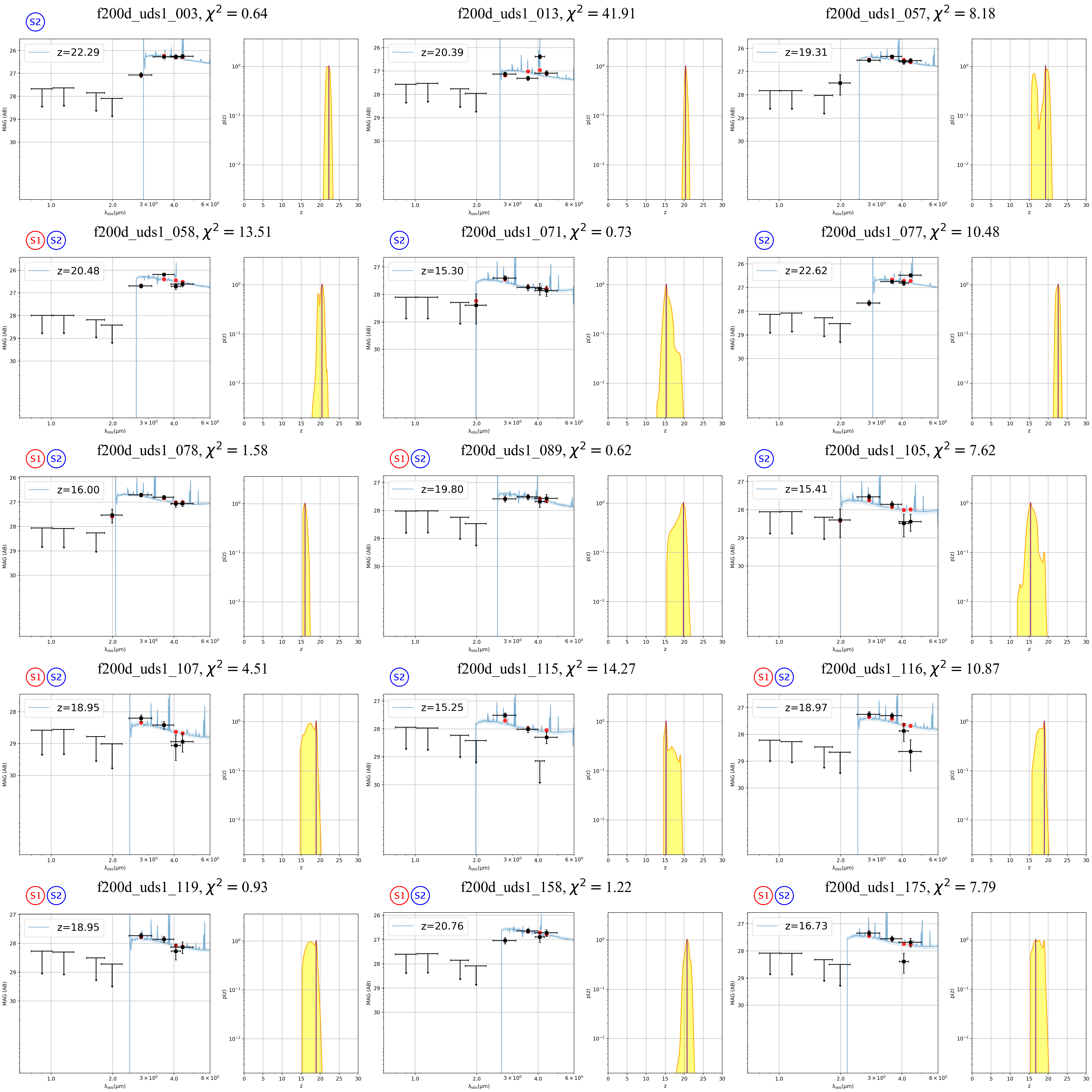
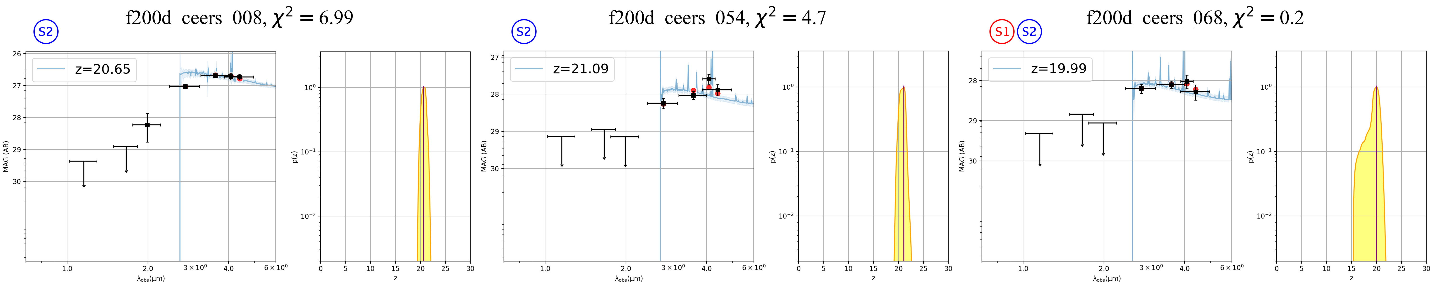
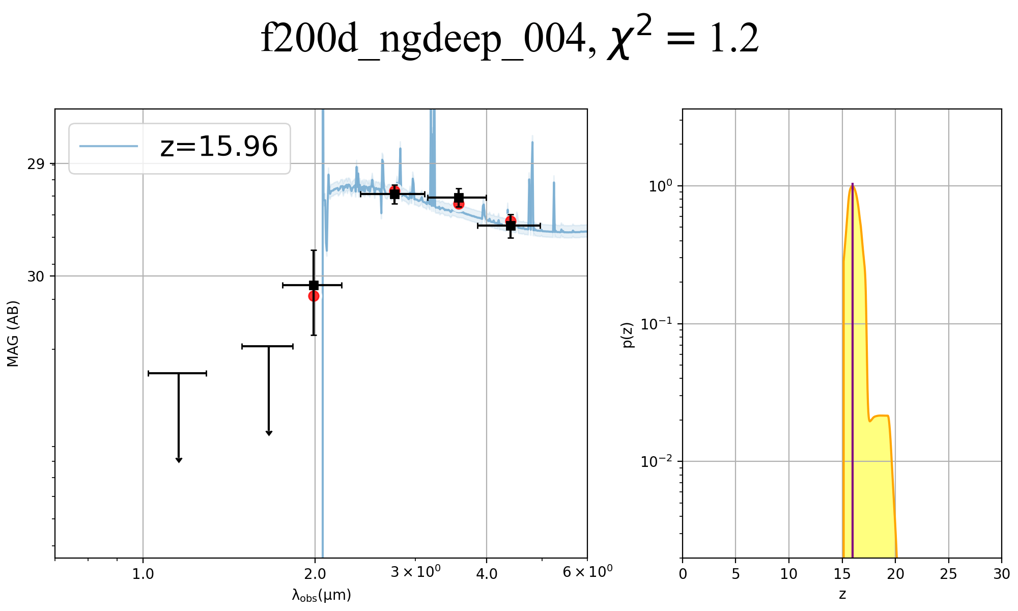
Figure A31: Same as Figure A21; for the F200W dropouts in UDS1, CEERS and NGDEEP.

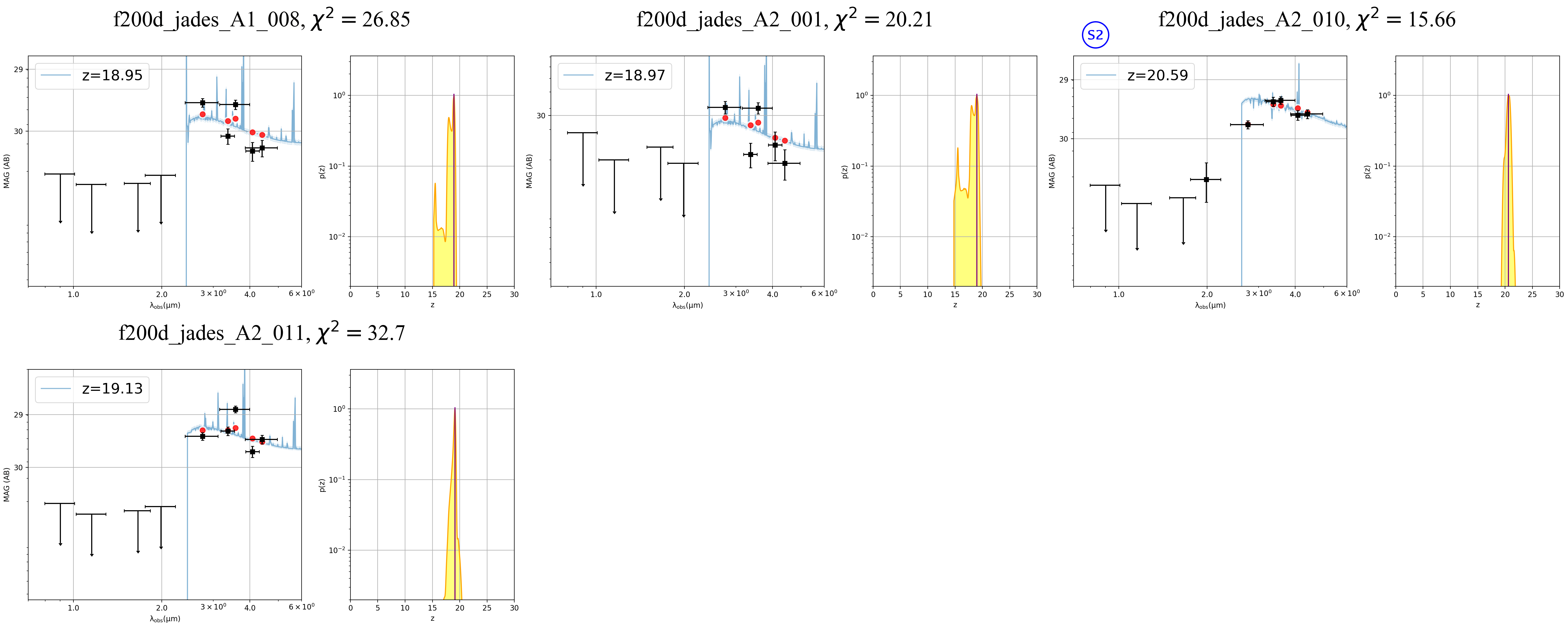
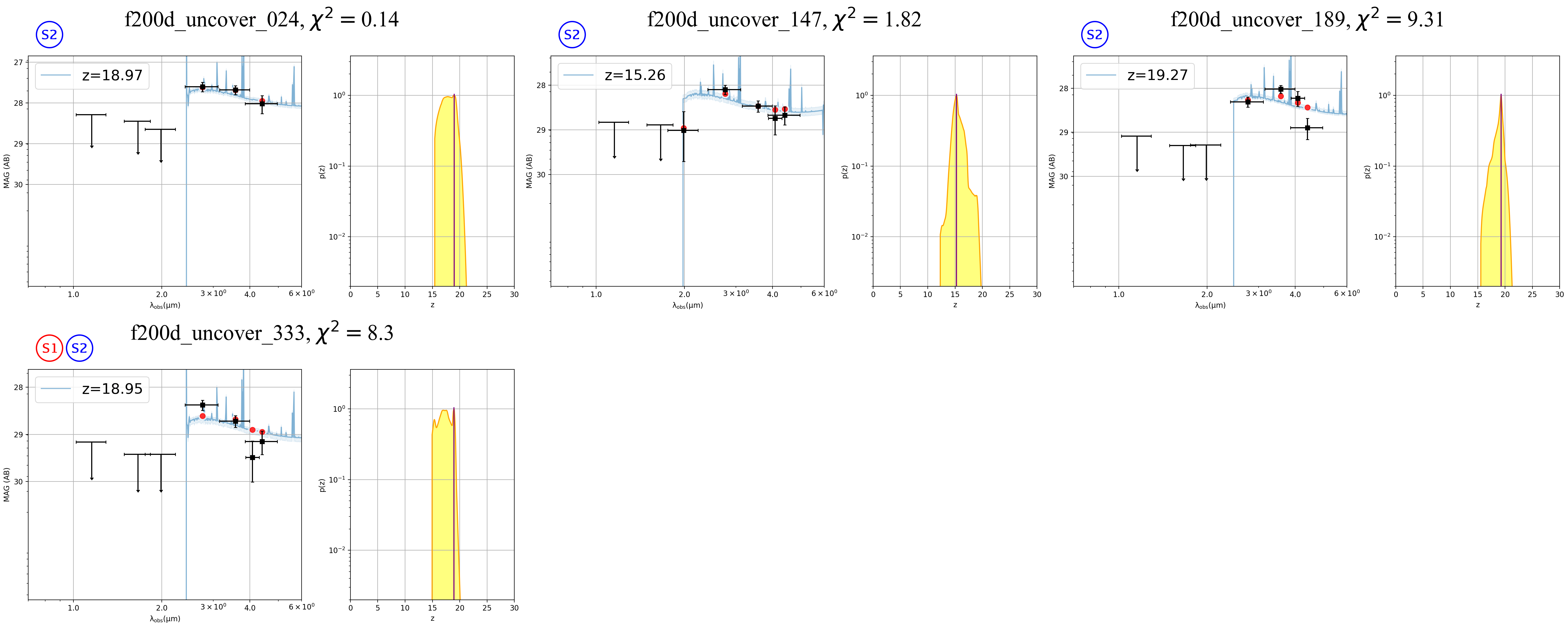
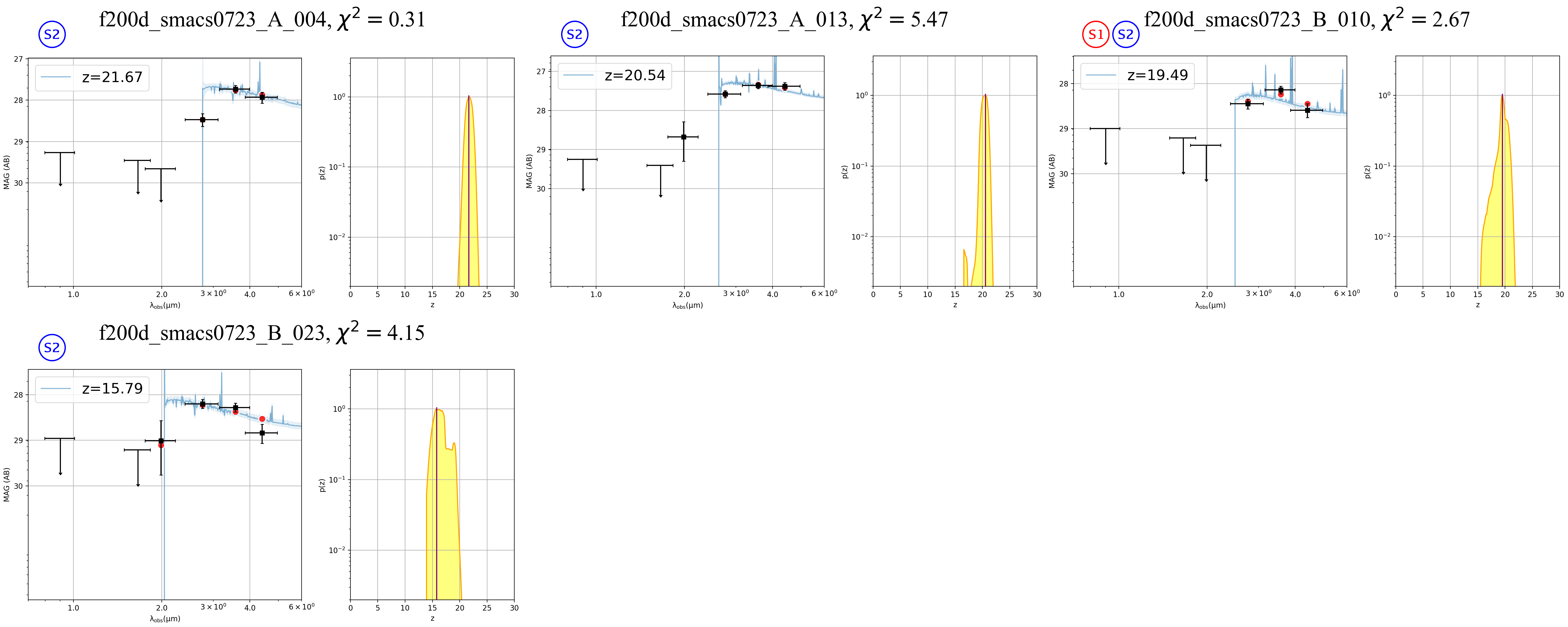
Figure A32: Same as Figure A21; for the F200W dropouts in JADES GOODS-S, UNCOVER and SMACS0723.

Appendix B “Depth Maps” for Effective Survey Area Calculation

As explained in Section 6.1, we calculate the effective survey area, $A_{\rm eff}$, for each of our dropouts individually. The total surface density of the dropouts found by a given survey is then the sum of the reciprocals of $A_{\rm eff}$. The implementation of the procedures outlined in Section 6.1 is as follows.

For a given survey, we first generate its 5 $\sigma$ and 2 $\sigma$ “depth maps” in all relevant bands using their RMS maps. Such a depth map gives the depth at each pixel, where the depth is calculated within a circular aperture of a certain radius. Using the depth maps, it is easy to find out whether a pixel is above the specified depth thresholds and therefore whether it contributes to the effective survey area of a given dropout. For illustration, let us use an F150W dropout with $m_{356}=29.25$ mag as an example. If a pixel in the F356W 5 $\sigma$ depth map is 29.25 mag or deeper, this pixel passes Step 1 in Section 6.1 for $A_{1}$ and goes to the next step.

Strictly speaking, the depth at each pixel should be calculated using the average of the pixels within the circular aperture centered at this pixel. However, calculating such a moving average over all pixels extremely time-consuming, and we simplify by assuming that the pixels within the aperture all have the same RMS value as the central pixel under question. The size of the aperture is somewhat arbitrary. Considering that we use a $r=$0$\farcs$2 aperture to calculate the 2 $\sigma$ limit when a candidate dropout is a non-detection in the drop-out band, here we adopt $r=$0$\farcs$2 as well for the depth map generation. A few smallest dropouts in our final sample have ISOAREA_IMAGE $<34.9$ pixels in the F356W 60mas mosaics, which means that the $r=$0$\farcs$2 aperture (occupying $\sim$34.9 pixels at the 60 mas scale) would be too large for them when calculating the depths, which would lead to an erroneously small effective area and thus an erroneously large density. For these dropouts, we generate the depth maps individually for each of them, with the aperture size tailored to occupy the same number of pixels as their ISOAREA_IMAGE.

References

- Adams et al. (2023a) Adams, N. J., Conselice, C. J., Ferreira, L., et al. 2023a, MNRAS, 518, 4755, doi: 10.1093/mnras/stac3347
- Adams et al. (2023b) Adams, N. J., Conselice, C. J., Austin, D., et al. 2023b, arXiv e-prints, arXiv:2304.13721, doi: 10.48550/arXiv.2304.13721
- Arnouts et al. (1999) Arnouts, S., Cristiani, S., Moscardini, L., et al. 1999, MNRAS, 310, 540, doi: 10.1046/j.1365-8711.1999.02978.x
- Arrabal Haro et al. (2023) Arrabal Haro, P., Dickinson, M., Finkelstein, S. L., et al. 2023, arXiv e-prints, arXiv:2303.15431, doi: 10.48550/arXiv.2303.15431
- Atek et al. (2023) Atek, H., Shuntov, M., Furtak, L. J., et al. 2023, MNRAS, 519, 1201, doi: 10.1093/mnras/stac3144
- Bagley et al. (2023) Bagley, M. B., Pirzkal, N., Finkelstein, S. L., et al. 2023, arXiv e-prints, arXiv:2302.05466, doi: 10.48550/arXiv.2302.05466
- Barrufet et al. (2023) Barrufet, L., Oesch, P. A., Weibel, A., et al. 2023, MNRAS, 522, 449, doi: 10.1093/mnras/stad947
- Behroozi et al. (2020) Behroozi, P., Conroy, C., Wechsler, R. H., et al. 2020, MNRAS, 499, 5702, doi: 10.1093/mnras/staa3164
- Bertin & Arnouts (1996) Bertin, E., & Arnouts, S. 1996, A&AS, 117, 393, doi: 10.1051/aas:1996164
- Bezanson et al. (2022) Bezanson, R., Labbe, I., Whitaker, K. E., et al. 2022, arXiv e-prints, arXiv:2212.04026, doi: 10.48550/arXiv.2212.04026
- Bowman et al. (2018) Bowman, J. D., Rogers, A. E. E., Monsalve, R. A., Mozdzen, T. J., & Mahesh, N. 2018, Nature, 555, 67, doi: 10.1038/nature25792
- Brammer et al. (2008) Brammer, G. B., van Dokkum, P. G., & Coppi, P. 2008, ApJ, 686, 1503, doi: 10.1086/591786
- Bruzual & Charlot (2003) Bruzual, G., & Charlot, S. 2003, MNRAS, 344, 1000, doi: 10.1046/j.1365-8711.2003.06897.x
- Bunker et al. (2023) Bunker, A. J., Cameron, A. J., Curtis-Lake, E., et al. 2023, arXiv e-prints, arXiv:2306.02467, doi: 10.48550/arXiv.2306.02467
- Calzetti (2001) Calzetti, D. 2001, PASP, 113, 1449, doi: 10.1086/324269
- Castellano et al. (2022) Castellano, M., Fontana, A., Treu, T., et al. 2022, ApJ, 938, L15, doi: 10.3847/2041-8213/ac94d0
- Chabrier (2003) Chabrier, G. 2003, PASP, 115, 763, doi: 10.1086/376392
- Curtis-Lake et al. (2023) Curtis-Lake, E., Carniani, S., Cameron, A., et al. 2023, Nature Astronomy, 7, 622, doi: 10.1038/s41550-023-01918-w
- Dekel et al. (2023) Dekel, A., Sarkar, K. C., Birnboim, Y., Mandelker, N., & Li, Z. 2023, MNRAS, 523, 3201, doi: 10.1093/mnras/stad1557
- Donnan et al. (2023) Donnan, C. T., McLeod, D. J., Dunlop, J. S., et al. 2023, MNRAS, 518, 6011, doi: 10.1093/mnras/stac3472
- Dunlop et al. (2021) Dunlop, J. S., Abraham, R. G., Ashby, M. L. N., et al. 2021, PRIMER: Public Release IMaging for Extragalactic Research, JWST Proposal. Cycle 1, ID. #1837
- Eisenstein et al. (2023) Eisenstein, D. J., Willott, C., Alberts, S., et al. 2023, arXiv e-prints, arXiv:2306.02465, doi: 10.48550/arXiv.2306.02465
- Ferrara et al. (2023) Ferrara, A., Pallottini, A., & Dayal, P. 2023, MNRAS, 522, 3986, doi: 10.1093/mnras/stad1095
- Finkelstein et al. (2022) Finkelstein, S. L., Bagley, M. B., Haro, P. A., et al. 2022, ApJ, 940, L55, doi: 10.3847/2041-8213/ac966e
- Finkelstein et al. (2023) Finkelstein, S. L., Bagley, M. B., Ferguson, H. C., et al. 2023, ApJ, 946, L13, doi: 10.3847/2041-8213/acade4
- Furtak et al. (2023) Furtak, L. J., Zitrin, A., Weaver, J. R., et al. 2023, MNRAS, 523, 4568, doi: 10.1093/mnras/stad1627
- Goulding et al. (2023) Goulding, A. D., Greene, J. E., Setton, D. J., et al. 2023, ApJ, 955, L24, doi: 10.3847/2041-8213/acf7c5
- Harikane et al. (2023) Harikane, Y., Ouchi, M., Oguri, M., et al. 2023, ApJS, 265, 5, doi: 10.3847/1538-4365/acaaa9
- Haslbauer et al. (2022) Haslbauer, M., Kroupa, P., Zonoozi, A. H., & Haghi, H. 2022, ApJ, 939, L31, doi: 10.3847/2041-8213/ac9a50
- Huang et al. (2011) Huang, J. S., Zheng, X. Z., Rigopoulou, D., et al. 2011, ApJ, 742, L13, doi: 10.1088/2041-8205/742/1/L13
- Ilbert et al. (2006) Ilbert, O., Arnouts, S., McCracken, H. J., et al. 2006, A&A, 457, 841, doi: 10.1051/0004-6361:20065138
- Inayoshi et al. (2022) Inayoshi, K., Harikane, Y., Inoue, A. K., Li, W., & Ho, L. C. 2022, ApJ, 938, L10, doi: 10.3847/2041-8213/ac9310
- Juodžbalis et al. (2023) Juodžbalis, I., Conselice, C. J., Singh, M., et al. 2023, MNRAS, 525, 1353, doi: 10.1093/mnras/stad2396
- Kannan et al. (2023) Kannan, R., Springel, V., Hernquist, L., et al. 2023, MNRAS, 524, 2594, doi: 10.1093/mnras/stac3743
- Larson et al. (2022) Larson, R. L., Hutchison, T. A., Bagley, M., et al. 2022, arXiv e-prints, arXiv:2211.10035, doi: 10.48550/arXiv.2211.10035
- Mason et al. (2023) Mason, C. A., Trenti, M., & Treu, T. 2023, MNRAS, 521, 497, doi: 10.1093/mnras/stad035
- McKinney et al. (2023) McKinney, J., Manning, S. M., Cooper, O. R., et al. 2023, ApJ, 956, 72, doi: 10.3847/1538-4357/acf614
- Meyer et al. (2023) Meyer, R. A., Barrufet, L., Boogaard, L. A., et al. 2023, arXiv e-prints, arXiv:2310.20675, doi: 10.48550/arXiv.2310.20675
- Mirocha & Furlanetto (2023) Mirocha, J., & Furlanetto, S. R. 2023, MNRAS, 519, 843, doi: 10.1093/mnras/stac3578
- Naidu et al. (2022) Naidu, R. P., Oesch, P. A., van Dokkum, P., et al. 2022, ApJ, 940, L14, doi: 10.3847/2041-8213/ac9b22
- Oesch et al. (2018) Oesch, P. A., Bouwens, R. J., Illingworth, G. D., Labbé, I., & Stefanon, M. 2018, ApJ, 855, 105, doi: 10.3847/1538-4357/aab03f
- Pascale et al. (2022) Pascale, M., Frye, B., Diego, J., et al. 2022, arXiv e-prints, arXiv:2207.07102. https://arxiv.org/abs/2207.07102
- Planck Collaboration et al. (2020) Planck Collaboration, Aghanim, N., Akrami, Y., et al. 2020, A&A, 641, A6, doi: 10.1051/0004-6361/201833910
- Pontoppidan et al. (2022) Pontoppidan, K. M., Barrientes, J., Blome, C., et al. 2022, ApJ, 936, L14, doi: 10.3847/2041-8213/ac8a4e
- Rieke & the JADES Collaboration (2023) Rieke, M., & the JADES Collaboration. 2023, arXiv e-prints, arXiv:2306.02466, doi: 10.48550/arXiv.2306.02466
- Rieke et al. (2023) Rieke, M. J., Kelly, D. M., Misselt, K., et al. 2023, PASP, 135, 028001, doi: 10.1088/1538-3873/acac53
- Robertson et al. (2023) Robertson, B. E., Tacchella, S., Johnson, B. D., et al. 2023, Nature Astronomy, 7, 611, doi: 10.1038/s41550-023-01921-1
- Rodighiero et al. (2023) Rodighiero, G., Bisigello, L., Iani, E., et al. 2023, MNRAS, 518, L19, doi: 10.1093/mnrasl/slac115
- Shen et al. (2023) Shen, X., Vogelsberger, M., Boylan-Kolchin, M., Tacchella, S., & Kannan, R. 2023, MNRAS, 525, 3254, doi: 10.1093/mnras/stad2508
- Treu et al. (2022) Treu, T., Roberts-Borsani, G., Bradac, M., et al. 2022, ApJ, 935, 110, doi: 10.3847/1538-4357/ac8158
- Vogelsberger et al. (2020) Vogelsberger, M., Nelson, D., Pillepich, A., et al. 2020, MNRAS, 492, 5167, doi: 10.1093/mnras/staa137
- Wang et al. (2023) Wang, B., Fujimoto, S., Labbe, I., et al. 2023, arXiv e-prints, arXiv:2308.03745, doi: 10.48550/arXiv.2308.03745
- Wang et al. (2016) Wang, T., Elbaz, D., Schreiber, C., et al. 2016, ApJ, 816, 84, doi: 10.3847/0004-637X/816/2/84
- Yan et al. (2023a) Yan, H., Ma, Z., Ling, C., Cheng, C., & Huang, J.-S. 2023a, ApJ, 942, L9, doi: 10.3847/2041-8213/aca80c
- Yan et al. (2023b) Yan, H., Cohen, S. H., Windhorst, R. A., et al. 2023b, ApJ, 942, L8, doi: 10.3847/2041-8213/aca974
- Yan et al. (2023c) Yan, H., Wang, L., Ma, Z., & Hu, L. 2023c, ApJ, 947, L1, doi: 10.3847/2041-8213/acc93f
- Yung et al. (2023) Yung, L. Y. A., Somerville, R. S., Finkelstein, S. L., Wilkins, S. M., & Gardner, J. P. 2023, MNRAS, doi: 10.1093/mnras/stad3484