Learning Regions of Attraction in Unknown Dynamical Systems via Zubov-Koopman Lifting: Regularities and Convergence
Abstract
The estimation for the region of attraction (ROA) of an asymptotically stable equilibrium point is crucial in the analysis of nonlinear systems. There has been a recent surge of interest in estimating the solution to Zubov’s equation, whose non-trivial sub-level sets form the exact ROA. In this paper, we propose a lifting approach to map observable data into an infinite-dimensional function space, which generates a flow governed by the proposed ‘Zubov-Koopman’ operators. By learning a Zubov-Koopman operator over a fixed time interval, we can indirectly approximate the solution to Zubov’s equation through iterative application of the learned operator on certain functions. We also demonstrate that a transformation of such an approximator can be readily utilized as a near-maximal Lyapunov function. We approach our goal through a comprehensive investigation of the regularities of Zubov-Koopman operators and their associated quantities. Based on these findings, we present an algorithm for learning Zubov-Koopman operators that exhibit strong convergence to the true operator. We show that this approach reduces the amount of required data and can yield desirable estimation results, as demonstrated through numerical examples.
Index Terms:
Unknown nonlinear systems, region of attraction, Zubov’s equation, Zubov-Koopman operators, regularity analysis, viscosity solution.I Introduction
An important aspect in dynamical systems is the determination of the region of attraction (ROA) for an equilibrium point. This is of significant importance in safety-critical industries such as aviation, robotics, and power systems, where comprehending operational boundaries is crucial.
Estimating the ROA for nonlinear systems can be rigorously resolved using formal methods [1]. Formal methods for nonlinear systems rely on a finite symbolic abstraction of the original systems. They can compute, with guaranteed precision for any arbitrarily small prescribed value, a set of initial states where the trajectories asymptotically reach an equilibrium point. Despite the precision of the estimation, formal methods entail rigorous abstraction analysis and face severe computational complexity arising from state space discretization. They are also not prepared for predicting the ROA of systems with limited knowledge.
This issue can be resolved by Lyapunov methods. Lyapunov functions qualitatively characterize stability properties for various nonlinear systems, and a forward-invariant sublevel set within their domains serves as an estimate of the ROA. The existence of Lyapunov functions is guaranteed by converse Lyapunov theorems [2, 3, 4, 5]. The primary challenge lies in the construction of Lyapunov functions that possibly enhance the conservative estimation of ROAs for more general nonlinear systems. On the other hand, Zubov’s theorem characterizes the maximal Lyapunov function [6] defined on the domain of attraction. However, it requires solving a partial differential equation (PDE) [7].
In real-world applications, limited knowledge of the system dynamics can make the identification of ROAs using Lyapunov methods even more challenging. Inspired by recent advances in Koopman operator-based system identification for unknown dynamical systems, we propose a Zubov-Koopman lifting approach to estimate the ROA by approximating the solutions to Zubov’s equations, whose non-trivial sublevel sets form the exact ROA. We aim to: 1) study the regularities of Zubov’s equation and introduce a linear Zubov-Koopman operator to characterize the solution; 2) configure the trajectory data and learn the Zubov-Koopman operator; 3) approximate the entire ROA for an asymptotically stable compact set, with emphasis on an asymptotically stable equilibrium point, using the learned Zubov-Koopman operator; 4) approximate near-maximal Lyapunov functions and provide formal verification as a byproduct.
We review some crucial results from the literature that are pertinent to the work presented in this paper.
I-A Related Work
The computation of Lyapunov functions has a long history [8] and has gained increased attention with respect to data-driven methods [9]. In particular, the development of the Koopman operator theory provides a promising alternative learning approach for nonlinear system identification and Lyapunov function constructions [10, 11, 12].
In essence, Koopman operators simplify the nonlinear analysis by lifting the states of the system into the space of observable functions, which evolve linearly governed by Koopman operators. The spectral properties of linear Koopman operators can facilitate Koopman mode decomposition for nonlinear systems using a specific set of observable functions. Several established techniques, such as dynamic mode decomposition (DMD) [13] and extended dynamic mode decomposition (EDMD) [14], can be employed to acquire this linear representation. In addition, the autoencoder architecture can be considered as suitable neural-network observable functions, although it requires more training efforts to achieve an optimized linear representation [15, 16].
Taking advantage of the spectral representation, in [17] and [18], the authors showed that a set of Lyapunov functions for nonlinear systems with global stability can be constructed based on the eigenfunctions of the learned Koopman operator. The work in [19] improved the multi-step trajectory prediction accuracy by a modified autoencoder architecture, with the corresponding Koopman eigenfunctions parameterizing a set of Lyapunov function candidates. In this framework, compared to the non-Koopman neural Lyapunov framework [20], it becomes possible to achieve a more desirable ROA estimation by exploring various valid combinations within the set of resulting Lyapunov functions.
The current Koopman analysis necessarily requires working on a forward-invariant compact subset within the state space. This allows the Koopman operators to preserve the associated function space on the invariant set. However, it sacrifices the ability to construct Lyapunov functions on a larger scale, given their unbounded nature near the boundary of the open ROA.
Considering this limitation, Zubov’s construction of a Lyapunov function seems to address the issue by ensuring that the solution is always bounded. This approach can offer potential advantages in numerical approximations, particularly when solving a PDE to find a Lyapunov function. This property enables the extension of the function domain to the entire state space or any desired set where computations occur [21].
In this regard, recent investigations have focused on numerical solutions to Zubov’s equation. In cases where system dynamics are known, the approach in [22] utilized local exponential stability conditions to train neural networks, similar in nature to physics-informed neural networks (PINNs) [23]. The most recent work [21] introduced PINN algorithms for computing Lyapunov functions capable of approximating the entire ROA for an asymptotically stable compact set with high accuracy. The Lyapunov function candidate generated by the neural network was also formally verified. The work in [24] employed a purely data-driven approach for estimating the solution to Zubov’s PDE. This method, however, requires long-term observation of trajectory data, and may have limited predictability of ROAs when the observation time is restricted.
I-B Contributions
Considering the pros and cons of the Koopman approach and Zubov’s PDE, we propose a Zubov-Koopman operator-based data-driven technique, leveraging trajectory data within a fixed observation span to predict the ROA of a known asymptotically stable compact set or equilibrium point for unknown dynamics. In brief:
-
1.
We conduct a regularity analysis for Zubov’s equation, where we relax the assumption from continuously differentiable vector fields to local Lipschitz continuity. Additionally, we explore how the solution to Zubov’s equation connects with a more general notion of Lyapunov functions.
-
2.
We introduce a Zubov-Koopman operator and establish its connections with Zubov’s equation. Building upon the regularity analysis mentioned earlier, we provide a detailed proof demonstrating how a Zubov-Koopman operator can lead to convergence to the solution of Zubov’s equation in a more general sense.
-
3.
While it is often assumed that finite-rank approximations apply to Koopman-like operators, we rigorously investigate the theoretical feasibility of finite-dimensional approximations for Zubov-Koopman operators and demonstrate how they can guide the selection of observable functions. Notably, the existing theorems on the existence of Koopman eigenfunction are either based on classical linearization theorems [25, 17] or complicated differential geometry [26] that is difficult to verify. The spectral analysis in this paper will focus on the specific goal of approximating the solution to Zubov’s equation under mild conditions.
-
4.
We introduce a learning algorithm for the Zubov-Koopman operator and employ the learned operator to approximate the solution to Zubov’s equation, thereby estimating the ROA. We show that extra efforts are required to obtain a near-maximal Lyapunov function.
-
5.
We provide numerical experiments and demonstrate the effectiveness of the proposed approach.
The rest of the paper is organized as follows. Section II presents some preliminaries on the Koopman operator, Zubov’s equation, and concepts for analyzing its solution regularity. Section III focuses on conducting regularity analysis under mild system conditions. Building on this, in Section IV, we introduce the Zubov-Koopman operator and demonstrate how the Zubov-Koopman operator can effectively characterize the solution to Zubov’s equation. Section V establishes the theoretical feasibility of a finite-dimensional representation of the Zubov-Koopman operator and demonstrates its interplay with observable data. Section VI introduces the algorithms, with numerical experiments conducted in Section VII. The paper is concluded in Section VIII.
I-C Notation
We denote by the Euclidean space of dimension , and by the set of real numbers. For and , we denote the ball of radius centered at by , where is the Euclidean norm. For a closed set and , we denote the distance from to by and -neighborhood of by . For a set , denotes its closure, denotes its interior, and denotes its boundary. For two sets , the set difference is defined by . For finite-dimensional matrices, we use the Frobenius norm as the metric. Given , we define .
Let be the set of continuous functions and be the set of bounded continuous functions with domain . We denote the set of -th continuously differentiable functions by , and similarly, bounded continuously differentiable functions by . We denote the set of locally and uniformly Lipschitz continuous functions by and . When making general statements for with , we denote as its gradient (or as the derivative when ).
II Preliminaries
II-A Dynamical Systems
Given a state space , we consider a continuous-time nonlinear dynamical system of the form
| (1) |
where denotes the initial condition, and the vector field is assumed to be locally Lipschitz.
On the maximal interval of existence , the forward flow map (solution map) should satisfy
| (2) |
Without loss of generality, throughout the paper, we will assume that the maximal interval of existence of the (unique) flow map to the initial value problem (1) is . We also generally consider that the state space , i.e., the flow is not necessarily assumed to be invariant within a strict subset of .
Let us now consider a complete, but not necessarily Hilbert, function space of the observable real-valued functions . The evolution of observables restricted on is governed by the family of Koopman operators, which are defined as follows.
Definition 1 (Koopman Operator)
The Koopman operator family of system (1) is a collection of maps defined by
| (3) |
for each , where is the composition operator. The (infinitesimal) generator of is defined by
| (4) |
where the observable functions should be within the domain of , i.e.
Suppose that the observable functions are bounded and continuously differentiable, the generator is such that
| (5) |
Koopman operators form a linear -semigroup that satisfies the following criteria. They allow us to study the nonlinear dynamics through the infinite-dimensional lifted space of observable functions with linear dynamics.
Definition 2 (Semigroup)
A one-parameter family , of bounded linear operators from into is a semigroup of bounded linear operators on if
-
1.
, ( is the identity operator).
-
2.
for every .
In addition, a semigroup is a strongly continuous semigroup, or -semigroup, if for all .
II-B Concept of Stability
We are interested in systems of the form (1) with an intrinsic asymptotically stable set . We define the set stability as follows.
Definition 3 (Set stability)
A closed invariant set is said to be asymptotically stable for (1) if
-
1.
for every , there exists a such that implies for all , and
-
2.
there exists a such that implies .
Furthermore, is said to be locally exponentially stable, if there exists a and such that , for all and
We further define the region of attraction (ROA) of given its asymptotic stability, which quantifies a region of the state space from which each absolutely continuous trajectory starts and eventually converges to the attractor itself.
Definition 4 (ROA)
Suppose that is asymptotically stable, the ROA of is a set defined as
Remark 5
It is a well-known result that the ROA is an open and forward invariant set.
To better convey the idea of this paper, we propose the following hypothesis for unknown systems in the form of (1).
-
(H1)
We assume that there exists an equilibrium point of (1), i.e. a point such that .
-
(H2)
We assume full knowledge of , and that is locally exponentially stable.
Based on Hypotheses (H1) and (H2), the purpose of this paper is to employ a data-driven approach to estimate the ROA of an equilibrium point of unknown systems.
II-C Zubov’s Theorem
The ROA can be characterized by a maximal Lyapunov function as described in the following theorem [6].
Theorem 6
Let be an open set. Suppose that there exists a function such that and the following conditions hold: 1) is positive definite on with respect to , i.e., for all and for all ; 2) the derivative of along solutions of (1) is well-defined for all and satisfies
| (6) |
where the function is continuous and positive definite with respect to ; 3) as or . Then .
Theorem 7
Let be an open set containing . Then if and only if there exists two continuous functions and such that the following conditions hold:
-
1.
for all and for all ;
-
2.
is positive definite on with respect to ;
-
3.
for any sufficiently small , there exist such that implies and ;
-
4.
as for any ;
-
5.
and satisfy (in the conventional differentiable sense)
(7)
Remark 8
Note that remains bounded, with its value approaching as approaches the boundary. In contrast, the function in Theorem 6 approaches infinity as approaches the boundary. The boundedness can offer significant advantages in data-driven approximations. In particular, it allows us to focus on a desired region of interest where computations occur. However, this modification is not as straightforward as it might appear. To better understand how Zubov’s construction can guide the data-driven approach to learning the ROA, we introduce an extension of Zubov’s theorem in Section III and rigorously examine the regularity of the solutions.
II-D Differentiability and Viscosity Solution
As we will see in Section III, the Zubov equation may not always possess differentiable solutions. One may need to consider a more general sense of solution to resolve.
Definition 9 (Viscosity solution)
Define the superdifferential and the subdifferential sets of at respectively as
| (9a) | |||
| (9b) | |||
A continuous function of a PDE of the form (possibly encoded with boundary conditions) is a viscosity solution if the following conditions are satisfied:
-
(1)
(viscosity subsolution) for all and for all .
-
(2)
(viscosity supersolution) for all and for all .
Remark 10
More details of viscosity solutions are provided in Appendix A. The concept of viscosity solution relaxes solutions. Note that, at differentiable points, exists and . In this case, to justify a viscosity solution, we can simply substitute and check if . If is not differentiable at a given point, then we have to go through the comparisons (1) and (2) in Definition 9 to verify that is a viscosity solution.
III An Extension of Zubov’s Theorem and Regularity Analysis
For the rest of this paper, we will assume that Hypothesis (H1) and (H2) hold and denote .
Inspired by (7) and its connection with through Eq. (8), to facilitate data-driven approximation, we explore the following dual form of Zubov’s equation (7), namely Zubov’s dual equation,
| (10) |
where
| (11) |
For now, we intentionally omit specifying the domain of and would like to discuss regularity analysis later in this section.
Note that, on , we always have . We prefer this dual form of Zubov’s equation because it allows us to potentially use a time series to approximate, as demonstrated in Section IV.
III-A Solution to Zubov’s Dual Equation
In this section, we construct the solution to the dual equation (10) of Zubov’s equation and demonstrate that, in a general context, it satisfies (10) in a viscosity sense.
Let be positive definite w.r.t. . Define
| (12) |
where if the integral diverges, we let . Then, we have the following property [21, Proposition 1].
Lemma 11
The function defined by (12) satisfies the following:
-
1.
if and only if ;
-
2.
as ;
-
3.
is positive definite with respect to .
Definition 12
Let . We further define
| (13) |
where . For test function , where for all , we denote for simplicity.
Remark 13
We would like to show that the construction in (13) is a solution to (10). Getting the conventional continuously differentiable solutions to (10) or (7) depends on the differentiability of (and hence the differentiability of w.r.t. ) and . However, this may not always be the case given the general assumptions on and . We provide a simple example below to demonstrate that we necessarily need to consider viscosity solutions to (10).
Example 14
Consider a simple dynamical system
and a convex, positive definite function . Then, it can be verified that for , as well as for and elsewhere. Clearly, for all and is not differentiable at and . Given the fact that is concave near , we also have that by [28, Chapter II, Proposition 4.7]. On the other hand, . For all , we have that , which show that satisfies (10) at in a viscosity sense. Similar proofs can be done at .
Lemma 15
Let Then, on , the function in (12) is a viscosity solution to with . In addition, if is also convex, then is a Lyapunov function on .
Proof:
It is clear that . On , by Lemma 11 and [21, Proposition 1], we have as well as the dynamic programming principle for all and . We now show that is a viscosity solution on using the equivalent conditions introduced in Appendix A. Let and be a local maximum point of . Then for all . For sufficiently small, we have . Therefore,
| (14) |
Considering the infinitesimal behavior on both sides of (14), i.e., dividing both sides by and taking the limit as , we have . The case when is a local minimum of can be proved in the same manner. Then, is a viscosity solution to on .
Remark 16
The above lemma extends the differentiability conditions of and in [30] to a more general setting, and shows the non-smooth Lyapunov property of . By Lemma 38 in the Appendix A and (15), even though the may not possess differentiability, there always exists a smooth Lyapunov function such that . Furthermore, from the above proof, one may notice that the sign of (or similarly, as in (16)) matters. In other words, is not a viscosity solution to .
Theorem 17 (Viscosity Solution)
Proof:
It is clear that and . For with , is automatically a differentiable and, hence, a viscosity solution to (16). We verify the case when .
On , since by Lemma 11, the inverse function () of is well defined. Since is a viscosity solution to , where is defined in Lemma 15, by [28, Chapter 2, Proposition 2.5], we immediately have that is a viscosity solution of . This implies that is a viscosity solution of (16) in . For , is always a viscosity solution.
It suffices to show the viscosity property on . Note that may not be differentiable on . However, by the famous Rademacher’s Theorem [31], is differentiable a.e. on each subdomain . Equivalently, satisfies
| (17) |
in the conventional sense, where . Now we introduce a smooth mollifier with compact support such that , as well as a kernel for . Then we define the convolution for by , and similarly for . It is clear that locally uniformly in . Convolve both side of (17) with , then,
| (18) |
Since is also linear in for any fixed , it follows that, for all ,
| (19) |
The following corollary shows the connection between (10) and (7) in the viscosity sense. The proof follows the same procedure as outlined above. We hence do not repeat.
Corollary 18
Theorem 19
Suppose that and are also locally Lipschitz continuous, then is the unique bounded viscosity solution to (16).
III-B Zobov’s Dual Equation on a Compact Subdomain
To facilitate data-driven techniques and prevent significant under-approximation of the ROA, we directly choose a sufficiently large compact region of interest . This region can either contain the entire ROA, assuming it is bounded, or cover a significant portion of the ROA if it is unbounded. Our proposed method uses observable data to recover the ROA relative to .
To incorporate Zubov’s dual equation, we need to recast the dynamics in . We first consider a first-hitting time of defined as follows,
| (21) |
It is clear that
-
1.
for all ;
-
2.
for all ;
-
3.
for all given that .
We further define stopped-flow maps so that one can observe the trajectories in .
Definition 20
Given the compact region of attraction , for each , we define the stopped-flow maps as
| (22) |
Note that in the above definition, the stopping time implicitly encodes the information of the starting position. It can also be verified that
-
1.
and for all , and
-
2.
for all .
We then consider a recast version of functions and (defined in (12) and (13)) accordingly. Let for all . For any 111Note that we have subtly changed the space of test functions from (in Eq.(13)) to ., define
| (23) |
where . For test function , we denote for simplicity. In this notion, it can be verified that if and only if and .
The following theorem collects nice properties of and on the refined region .
Theorem 21
For any ,
-
1.
is a viscosity solution to
(24) on , where is defined in (11). Suppose that and are also locally Lipschitz continuous, then is the unique bounded viscosity solution.
- 2.
-
3.
Let On any invariant set , the function is a viscosity solution to with . In addition, if is also convex, then is a Lyapunov function.
Proof:
The proof follows a similar procedure as the proofs of the statements in Section III-A. Indeed, the proof should be the same for any such that . Particularly, the dynamic programming as in the proof of Lemma 15 still holds given the flow map property of . For any such that , the solution is trivial considering that the quantity diverges. ∎
Remark 22
By Theorem 21, suppose that , one can only recover a portion of that is not absorbed by the boundary by solving (24). This portion should be a sublevel set (relative to ) of the . In view of [33, 34, 35], this sublevel set is also a subset of the refined open and invariant subregion of ROA, from which trajectories will satisfy the reach-avoid-stay property.
IV Zubov-Koopman Operators and Semigroup Property
Addressing the problem of estimating the ROA, we have introduced Zubov’s dual equation as well as its refined form on . The solution involves an improper integral up to , which requires nearly the full knowledge of the trajectory [24]. To reduce the substantial amount of observation data, in this section, we derive an approximation approach using a time series. Specifically, this time series is governed by a convergent, time-homogeneous, and Feynman-Kac like semigroup, which allows us to approximate the long-term behavior through a simple iterative process.
We first work on and then on the refined region .
IV-A Introducing Zubov-Koopman Operators
Consider
| (25) |
and, for any and , we define as
| (26) |
The following proposition shows the basic properties of . We complete the proof in Appendix C.
Proposition 23
is a -semigroup. In addition, for each and for any , for all .
The stochastic version of is the famous Feynman-Kac semigroup [36, Chapter 8]. While this is generally not true for stochastic systems, for deterministic systems, we observe that depicts a form of separation of variables and can be written as a multiplication of a contraction operator with the Koopman operator, i.e. . The following theorem also shows a close connection with the Zubov’s eual equation. For the purpose of using the flow of governed by to approximate the solution of Zubov’s dual equation, for any fixed , we name as the Zubov-Koopman Operator.
Theorem 24
Let the test function be . Suppose that is nonnegative. Then
-
(1)
solves the following Cauchy problem, for all and all ,
(27) -
(2)
Conversely, for any that satisfies (27), the solution should be of the form .
Proof:
Note that the (infinitesimal) generator of the Koopman semigroup acting on is such that
To prove (1), we first look at how evolves according to for some small . By the definition of , for any fixed , we have
| (28) |
Note that
| (29) |
Sending on both sides, it follows that
which completes the first part of the proof.
To prove (2), we suppose that solves (27), then
and for all . Introduce an auxiliary function . Then it is clear that . However,
where the quantity is defined as in (25). Therefore, the quantity is a constant for all and , which implies that
The proof is completed. ∎
IV-B A Time-Series Approximation
Clearly, by the definition of in (13), for any , we have that for all . In particular, uniformly, and is also the unique, up to multiplicative constants, fixed point of . To approximate , one can pick a fixed time interval , and define
| (31) |
as well as
| (32) |
Then, by (13) and the uniqueness (up to multiplicative constants) of the fixed point, the composed operator for any , and for any such that . Suppose that one can approximate properly, then for some large should be a reasonably good approximate for .
Similar to the approximation of Koopman operators, to obtain a discrete version of the bounded linear operator , it usually relies on the choice of a (discrete) dictionary of observable test functions, denoted by
| (33) |
Then, the approximation is valid in the sense that, for each , there exists an and a uniformly continuous residual term such that
| (34) |
Possible choices of the dictionary have been discussed in [14, 19], including polynomials, Fourier basis, spectral elements, and neural network-based functions. These choices are generally locally Lipschitz continuous, but there may be cases where differentiability is not exhibited, as seen in neural network-based functions with ReLU as the activation function.
In line with Theorem 24 and viscosity regularity of Zubov’s dual equation, to make the time series approximation of robust, we extend Theorem 24 for test functions and verify the regularity.
Theorem 25
Let the test function be . Suppose that is nonnegative and locally Lipschitz. Then, for each , is the unique viscosity solution to (27).
Furthermore, for each fixed , suppose that there exists a family of functions and, accordingly, a family of uniformly bounded continuous residuals with Lipschtiz constant , such that
and . Assume on each bounded subdomain . Then, as , converges uniformly to .
In addition, suppose we also have , then the function is the unique viscosity solution to with , where (as ) on each bounded subdomain .
Proof:
Since the proof of viscosity property is similar to the proof for , we omit the first part of the proof.
Now, as , by the uniform convergence of for any , one has uniformly converges to on each subdomain . By the construction of , as , also uniformly converges to . Therefore, for each , uniformly, which completes the second part of the proof.
By the construction of , and by the first part of Theorem 25, we can immediately have that, for each and for each , is the unique viscosity solution to
| (35) |
Since is necessarily locally Lipschitz continuous, exists a.e.. At a differentiable point, we have
The above implies that converges uniformly to a.e.. For sufficiently large and , by a similar argument as the first part222One can take a convolution on both side of (35) with a mollifier and let . Then satisfies the requirement. , one can verify that there exists an such that and is the viscosity solution to
| (36) |
By a similar argument as in Proposition 15, given the smoothness of , there exists an with such that is the unique viscosity solution to with . ∎
Remark 26
The first two parts of the above theorem state that, even though we may only use a family of uniformly convergent locally Lipschitz functions to approximate, the limit still satisfies (27) is a viscosity sense. In addition, we can find a proper approximation for . For the purpose of approximating ROA, this approximation is satisfactory.
On the other hand, without the assumption that , the approximation may not solve (35) with vanishing in a proper sense. This may eventually cause the third part of the statement to fail to hold, meaning that the approximation can not be readily used as a Lyapunov function. We will also demonstrate this effect in Section VII via examples.
At the end of this section, we make a quick extension of the aforementioned results, further refining our observations on the compact region of interest . Due to the similarity with previous results, we omit the proof for the following Corollary.
Corollary 27
Recall the stopped-flow map defined in Definition 20. Let . For any and , we redefine as
| (37) |
Then,
-
1.
is a -semigroup.
-
2.
For each each and for each , is an eigenfunction such that .
-
3.
For any test function , given that is nonnegative, then is the unique viscosity solution to (27) for all and .
-
4.
Suppose there exists a family of functions that uniformly converges to for any , then, as , converges uniformly to , where is defined in (23).
-
5.
Suppose we also have , which is the Lipschitz constant for for each . Then, for sufficiently large and , the function is the unique viscosity solution to with on any invariant set , where is arbitrarily small.
Remark 28
We have chosen not to introduce the ‘hat’ notation for the redefined in (37). We encourage readers to verify the space of the test functions before using .
V Finite- Dimensional Approximation of Zubov-Koopman operators.
As we have seen in (34), we expect to find an approximation for the Zubov-Koopman operators such that the image functions converge uniformly. In practice, we would like to see if the training discrete dictionary (as in (33)) of observable test functions can be reduced to finite, such that the approximation behaves like a finite-rank operator, and preserves for some .
In this section, we rigorously investigate basic properties and a finite-dimensional approximation of Zubov-Koopman operators. We will work on the compact region of interest for the rest of this paper. Since our purpose is to learn Zubov-Koopman operators based on training data, we propose a three-step intermediate approximation for , such that for any , an approximation of the form (34) holds.
V-A Compact Approximation of Zubov-Koopman
defined in (37) is clearly a family of bounded linear operators. One may attempt to show that is also compact for each . It suffices to show that is relatively compact, where for some . However, equicontinuity within is not guaranteed. To see this, we set (or similarly, the Fourier basis), and let for all and elsewhere. Then, the sequence for each does not possess equicontinuity due to the rapid oscillation as increases.
Nonetheless, the following proposition states that one can use compact operators to strongly approximate for each .
Proposition 29
For each , there exists a family of compact linear operator , such that for all , we have as .
Proof:
For each , we rewrite the Koopman operator as , where is the Dirac delta. Now we use a family of integral operators with smooth kernels to approximate the above distribution. The idea is to approximate the Dirac delta using a smooth mollifier as we have seen in the proof of Theorem 25. For each , let and . It can be verified that with a compact support in . We define the approximation as for all . It is a well-known result that, for each and , the operator is compact given its smooth kernel.
To verify the convergence property, the rest of the proof falls in a standard procedure. Now, for each and all , by change of variable, we have that . It follows that
| (38) |
Note that, tor each , given any and any Lipshitz continuous map , the composition is a uniform continuous function on . Therefore, by definition, is also uniformly continuous on . The last term above converges to as for all . Therefore, for each , taking the supremum on both sides of (38) and sending to , we have . ∎
Corollary 30
For each , there exists a family of compact linear operator , such that for all , we have as .
Proof:
Remark 31
The convergence in Proposition 29 cannot be extended to the convergence w.r.t. the operator norm, i.e. . One may revisit the example for . It is clear that for all , but based on the inequality in (38), the uniform limit fails to exist due to the unbounded Lipschitz constants of . However, for the purpose of this section, the convergence in Proposition 29 is already satisfactory.
V-B Finite Dimensional Representation
Since the kernels of are smooth and compactly supported, it is a well-known result that the operators within this family are Hilbert-Schmidt operators.
We then investigate the spectral behavior of within a separable Hilbert space with the inner product . Let be the eigenfunctions of . Then, for all , we have that as well as where are the corresponding eigenvalues in the -scale.
Remark 32
In the above infinite-sum representations, we have implicitly assumed that the eigenfunctions are real-valued. However, this is not always the case. For more general situations, for all , and as well as . For simplicity, we still use the above expressions without further indicating whether they are real or complex-valued.
Proposition 33
For any fixed , for any arbitrarily small , there exists a sufficiently large and a finite-dimensional approximation such that
Proof:
The Hilbert-Schmidt operator is also necessarily a finite-rank operator, i.e., for any complete orthonormal basis , . Denoting the finite truncation as , we have for all . Combining Proposition 29, we have the desired property. ∎
Remark 34
In contrast to the approach described in [37, Section III, 2)], wherein the finite-rank operator is limited to preserving only a finite-dimensional subspace of the initial function space, our proposed finite-rank approximate operator, as in Proposition 33, demonstrates better theoretical robustness. Notably, it retains a valid infinite-dimensional domain, i.e. , identical to that of for all .
Particularly, suppose are complex-valued and is the solution to (10), by the eigenvalue problem in Proposition 23, we have that and for some such that . Then, the corresponding is an approximation of the eigenvalue of , but the eigenfunction is not a direct approximation for . We still need the expansion form to properly approximate .
V-C Feasibility of Data-driven Approximation
For any fixed , based on Proposition 33, the original operator (recall Definition 31 for ) can be approximated (strongly) with an arbitrarily high precision by a finite-dimensional bounded linear operator , which preserves the non-ignorable eigenmodes. We would like to further use a data-driven approach to learn the eigenvalues and the eigenfunctions for this finite-dimensional operator.
To do this, we consider a sufficiently dense -dimensional subspace and choose observable test functions from . Then, , where represents the vector of the projection inner products. If is also dense in , then this finite-dimensional approximation is of the desired form as in (34).
Suppose that is given arbitrarily, then each may not be invariant within under . However, when restricted on the -dimensional truncation, the approximate operator preserves the space . We aim to express by functions from .
Taking advantage of the linear transformation, for systems with unknown dynamics, data-driven methods will approximate the Zubov-Koopman eigenvalues and eigenfunctions by fitting the data and for some . We also denote by the stack of input and output data. The best-fit matrix is formulated as an optimization problem
Similar to EDMD [14], the learned operator has the following sense of approximations.
-
1.
Let be the eigenvalues and eigenvectors of . Then, for each , the learned eigenvalues is such that , and the learned eigenfunction satisfies . 333The eigen-approximation is only for the compact operator introduced in Section V-A. The original operator may not possess non-trivial point spectrum other than .
-
2.
For any such that for some column vector , we have that
(39)
By the well-known universal approximation theorem, all of the function approximations from above should have uniform convergence.
VI Data-driven Algorithms
By the finite rank expansion (39), one can easily verify that
| (40) |
where is such that . By virtue of Proposition 23 and Corollary 27, for all , the real-valued eigenfunction of with the corresponding eigenvalue should be , up to multiplicative constants. Similarly, the only non-vanishing mode(s) as should be the ones with , which will be readily a solution to the Zubov’s dual equation suppose it is real-valued. If this happens, we can directly choose associated with as the approximation for without any iteration. However, due to the numerical error and the possibly complex-valued eigenvectors of , one still needs to use the iteration form for some sufficiently large as the final approximation.
Nonetheless, the key is to learn using observable data of trajectories within a relatively shorter time period, and obtain the matrix so that the (40) can be utilized. To do this, we modify the existing Koopman learning techniques for Zubov-Koopman operators , as defined in (31), with a fixed training time interval .
VI-A Generating Training Data
As we have briefly discussed about the feasibility of using data-driven approaches to approximate the operator for each and each , we consider as the features and as the labels. We inevitably need to acquire the stopped-flow map and compute the integral. Drawing inspiration from [24], for each termination time, we can assess both the trajectory (without stopping) and the integral, i.e. the pair , by solving a single augmented ODE system
| (41) |
We propose the following algorithm based on this technique for our purpose of evaluating for each and each .
Algorithm 1
Let the region of interest , the dictionary , the function , and the time interval be given. Then, for each and , we compute as follows.
- 1.
-
2.
(Identifying out-of-domain index) Identify the first element numbered as in that is not within .
-
3.
(Identifying the intersection point on the boundary) If , continue to the next step. Otherwise, find the line segment connecting the -th and -th elements (i.e. and ). Find the intersection point of the line segment and .
-
4.
(Modifying the trajectory and the integral) If , continue to the next step. Otherwise, for each , replace by , and replace by . Keep the notation for the modified and .
-
5.
.
We summarize the algorithm for generating training data for one time period in Algorithm 2.
VI-B EDMD Algorithm for Operator Learning
After gathering training data, the rest of the training process should be the same as the existing Koopman operator learning techniques. We perform the EDMD algorithm to obtain the final approximation for .
EDMD algorithm provides an estimation of using one time period observation data. We use Algorithm 2 to obtain training data . As we have briefly discussed in Section V-C, we need to find in order to obtain the approximation of the form (39). For EDMD, the is given in closed-form as
| (42) |
where is the pseudo inverse.
VI-C Predicting ROA and Constructing Lyapunov Function
To predict , Eq (40) is also ready to use. We simply pick a tolerance and the largest number of iteration , then iterate until reaches the threshold or , whichever comes first. For simplicity, we can also choose the dictionary to include a real-valued such that . Then, we obtain a Zubov-Koopman approximation of ,
| (43) |
where is the -th standard basis vector. Since and are uniformly close, we can approximate the ROA by the largest connected positive level sets of .
As for constructing a Lyapunov function, in virtue of (35) and Remark 26, we may not directly use the result just yet. Fortunately, by the viscosity regularity of and the alternative comparison principles given in Lemma 38, one can seek a smooth function that uniformly approximates , and hence uniformly approximates , with its Lipschitz constant also converges to that of .
We achieve this extra modification by neural networks (NN) using a new set of samples (could be different from the one used in Algorithm 2) and . This NN approximation will be named . We omit this algorithm as it follows the standard procedure. The formal verification of utilizes satisfiability modulo theories (SMT) solvers and follows the exact procedures in [21, Section V].
Remark 35
Note that for any Lipschitz continuous function, the Lipschitz constant of its smooth neural approximations typically converges to the true Lipschitz constant. This phenomenon has been extensively studied by [38]. When verifying the Lipschitz constant of the residual is challenging, assuming this phenomenon holds is reasonable.
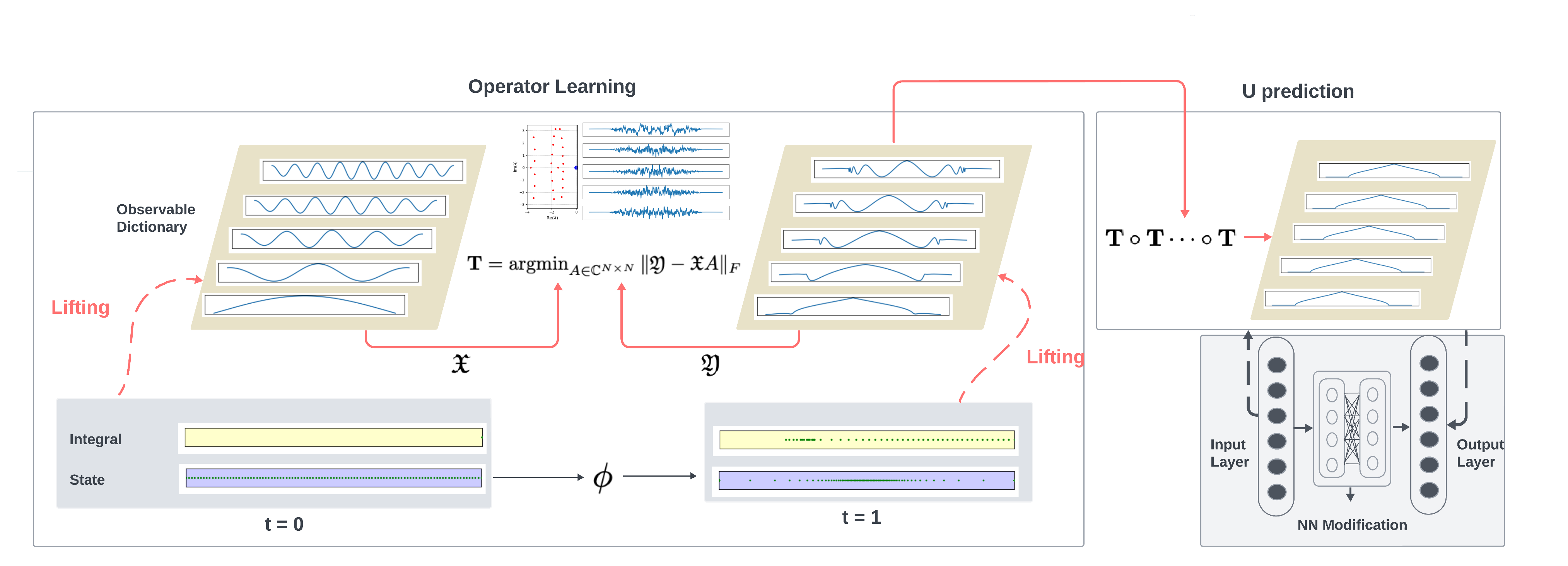
We summarize the learning procedures in Fig. 1.
VII Numerical Examples
In this section, we provide numerical examples to demonstrate the proposed Zubov-Koopman approach for predicting ROAs, as well as learning and verifying neural Lyapunov functions. For consistency, the reported computation times were recorded on a MacBook Pro equipped with a M1 Pro 10-Core CPU and 32GB of memory. Multiprocessing was applied to all the examples, and the recorded calculation times for smaller data volumes can deviate from real values due to computational overhead. Code for the numerical examples can be found at https://github.com/Yiming-Meng/Zubov-Koopman-Operator-Learning.
VII-A One-dimensional Nonlinear System
We revisit Example 14 and explain the effectiveness of the Zubov-Koopman approach. Consider the dynamical system
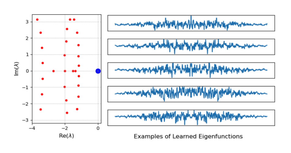
and . We would like to find the ROA of and a valid Lyapunov function using the trajectory data up to within the region of interest . We sample for , and use the dictionary for , where We execute Algorithm 2 to prepare the training set, which takes seconds. We obtain the discrete operator as in Section VI-B, which requires seconds. The spectrum (-scale) and the first learned functions (of as defined in Section V-A) are shown in Fig. 2. We can clearly see the spectral gap between the top eigenvalue (in blue) and the rest of the point spectrum.
Remark 36
For each , . As discussed in Section IV-B, we have . We simply pick as for our purpose. Furthermore, the choice of is in consideration of the periodicity of the (stopped) trajectories in . One can also replace it with Fourier basis. The multiplication with is for smoothing the high-frequency observables functions.
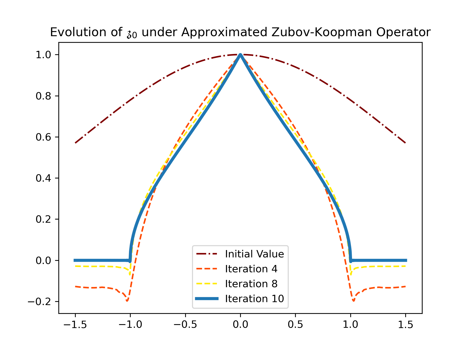
Using the learned matrix , we first show the evolution of governed by the approximation of , i.e., we obtain , where , for a sequence of . We observe the trend of convergence as in Fig.3.
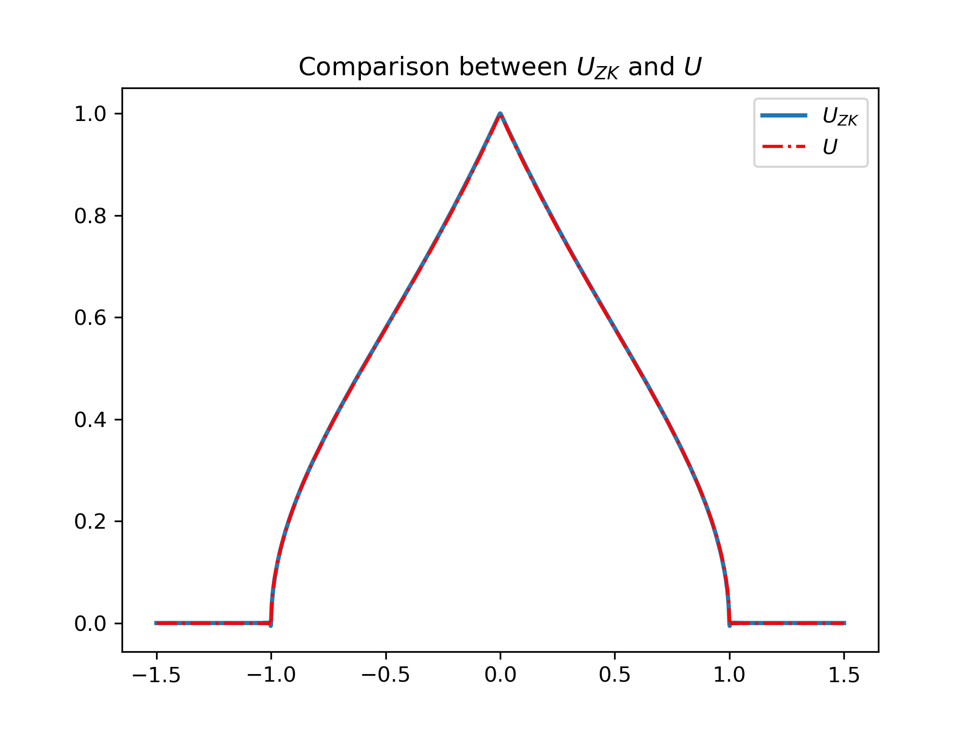
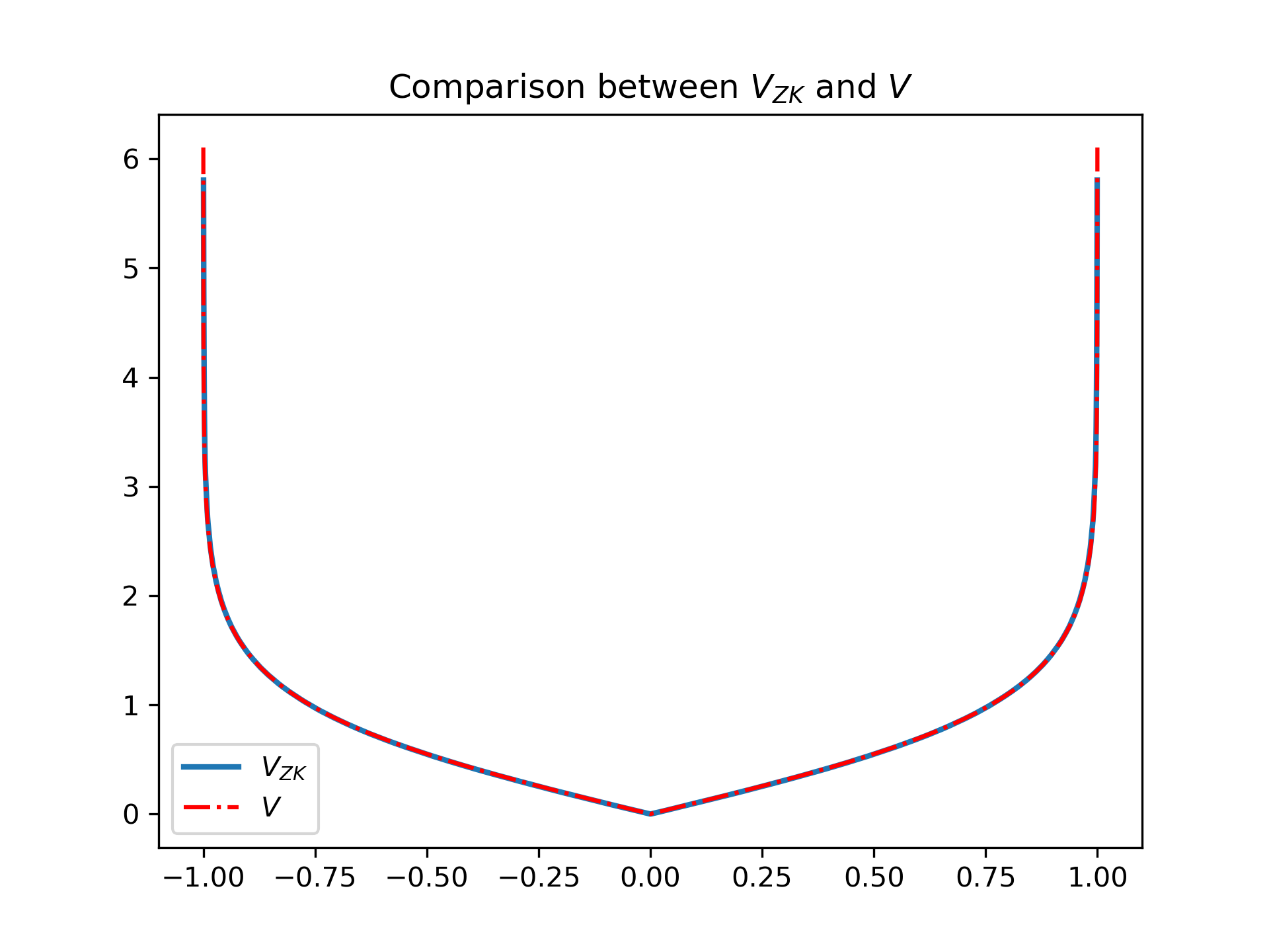
After the -th iteration, we have that . Now we let and obtain that the largest connected positive level sets of is , which is approximately . On this domain, we set . Then, we compare the and with the true and defined in Example 14 as in Fig.4. It can be inspected that both approximations achieve a high accuracy. The under-approximation of the ROA is due to the tiny oscillation near the boundary points .
Remark 37
To see whether can serve as a Lyapunov function, we proceed to verify if the numerical error can still make (or equivalently, ). The comparisons with the true functions are provided in Fig. 5.
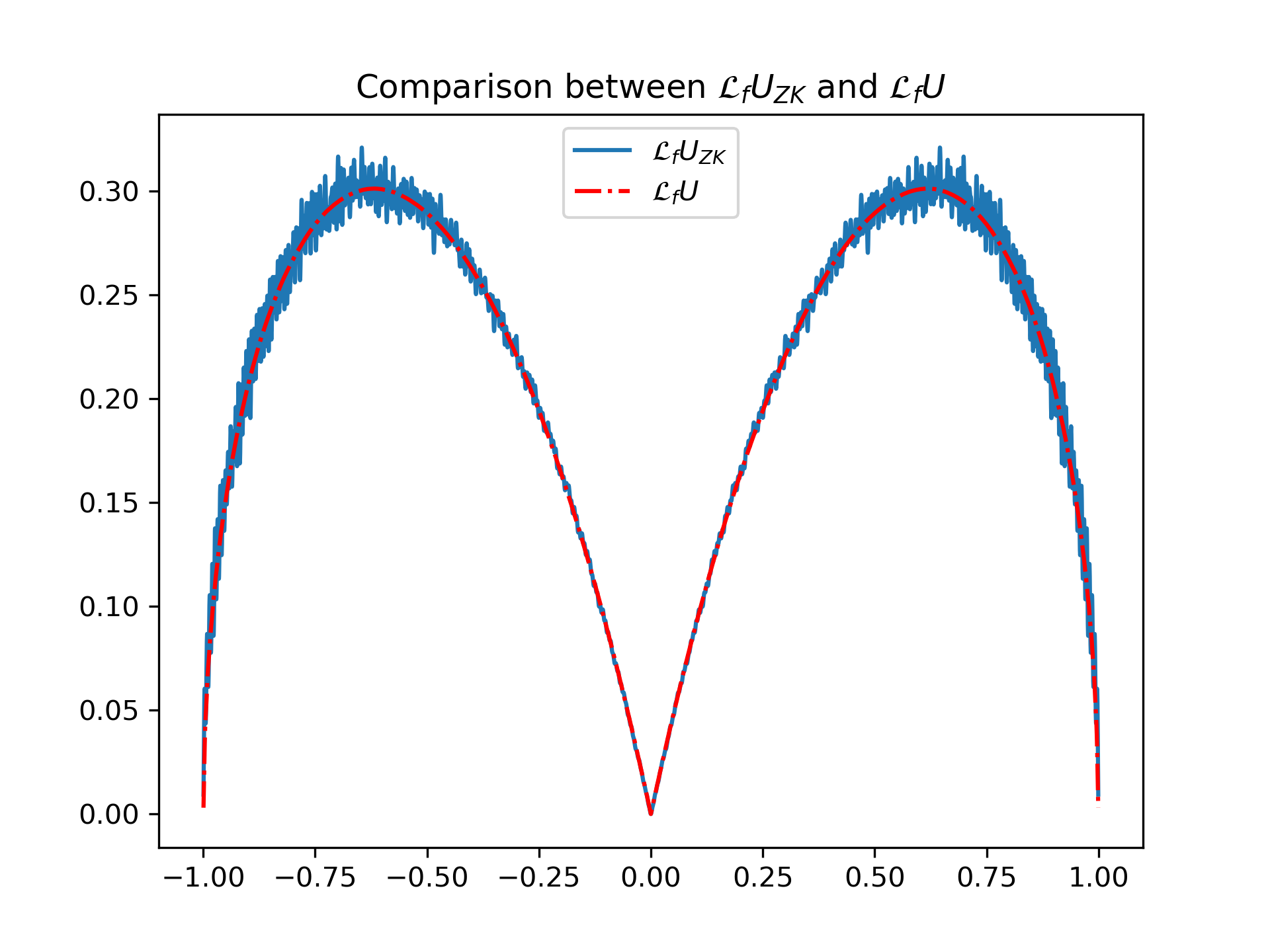
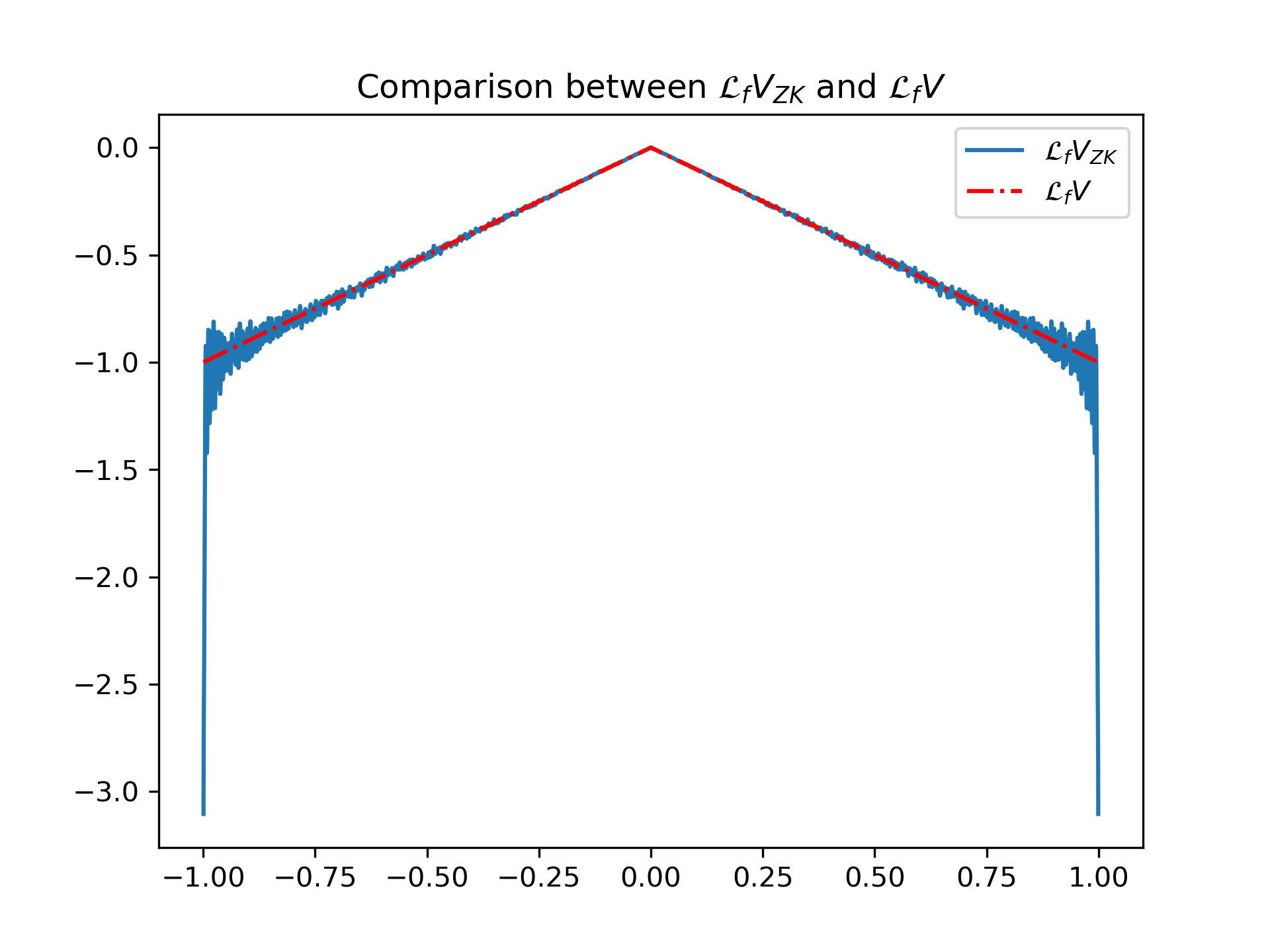
The approximations for and are not as accurate as those for and due to the high-frequency decomposition. However, the approximate quantities are verified to preserve the sign on , which is the valid sub-domain to use as a Lyapunov function. We hence do not have to use an extra NN-modification for the construction.
VII-B Reversed Van der Pol Oscillator
Consider the reversed Van der Pol oscillator
with . The system has a stable equilibrium point at . We use this example to compare the data efficiency of predicting the ROA of as well as finding a Lyapunov function between the Zubov-Koopman approach and the data-driven approach presented in [24].
In this example, we set , and pick the region of interest as . A total of , , and uniformly spaced samples in are generated respectively for three parallel experiments.
VII-B1 Zubov-Koopman method
We simulate the trajectory up to . The dictionary is selected in a similar manner as in the one-dimensional example with adjustments for two-dimensional inputs, i.e., we set for each and . We let , which means a total of observable basis functions are used. To obtain through iterations, we set the termination tolerance to with a maximum of iterations. The prediction of the ROA (or ) follows the same procedure as in Section VII-A.
For the construction and verification of a Lyapunov function, we need to incorporate an additional NN modification, as described in Section VI-C, due to inaccuracies in the derivatives of . The training set should be independent of the one used for obtaining . Therefore, for all the experiments at this stage, we use uniformly spaced samples, along with the evaluations of at those points, to train . We use a network with hidden layers, each containing 15 neurons. We terminate training when the mean-square training loss was smaller than or after epochs.
VII-B2 Data-Driven method
As for the data-driven method in [24], for each experiment, we use the same samples as above and generate trajectory data up to a termination time , or until . We then use and to train a neural-network . We use a network model with hidden layers, each containing 15 neurons. We terminate training when the mean-square training loss is smaller than or after epochs. We predict the ROA as the largest connected positive level sets of . This neural solution is also ready to be verified as a Lyapunov function without extra modification.
VII-B3 Verification
Please note that the approximations and are intended for Zubov’s dual equation, not the original equation. To ensure consistency with the procedure for verifying the neural Lyapunov functions as described in [21], it is important to pay attention to sign conversion.
VII-B4 Experiment results
The comparison results are reported in Table I. In the table, ‘IVP solving’ corresponds to steps 1) to 4) of Algorithm 1, while ‘stacking’ involves preparing the data for learning. For the Data-Driven method, ‘function learning’ refers to the NN training, whereas for the Zubov-Koopman approach, it pertains to the iterative procedure to obtain (see (43)). We also recorded the NN final losses for both approaches whenever a neural network was employed during the process.
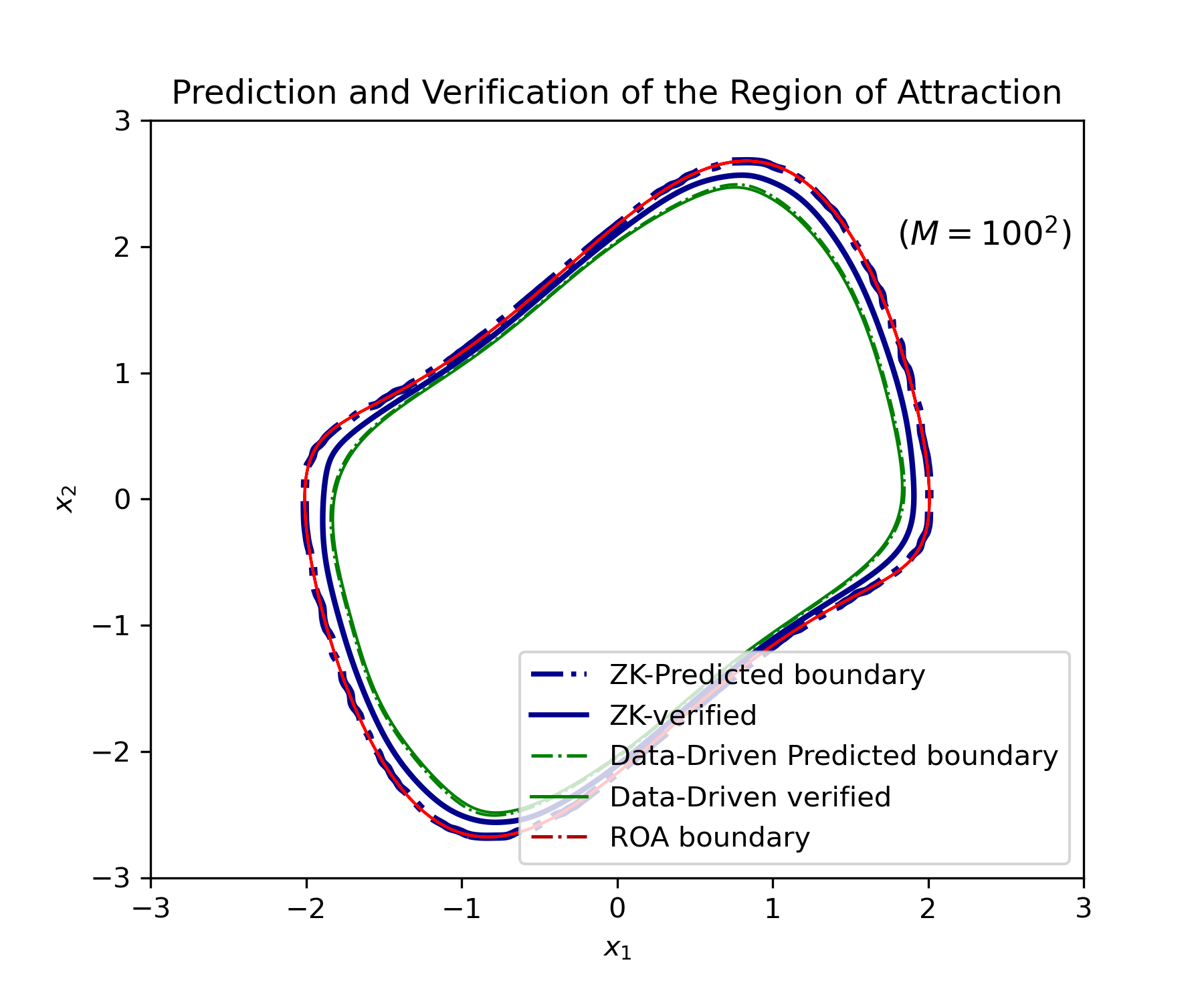
We show the predicted and verified boundaries of the ROA for in Fig. 6. The prediction using the Zubov-Koopman approach shows overall better accuracy, while the verified regions are similar for all the methods. On the other hand, with initial samples, the region verified by the Data-driven method is slightly smaller. This is because the verification relies on NN approximation for both methods, but the Zubov-Koopman approach’s NN stage is based on an already good approximation of , which is not constrained by the initial sample size. These phenomena also reflect that the and the data generated for the Data-driven method have similar quality in cases where and .
| Approaches | Sample size | IVP solving time | Stacking time | Operator learning time | Function learning time | Modification time ( samples) | NN final loss | Verified volume |
| Data-driven | 10.13(s) | 0.81 (s) | - | 54.24(s) | - | 84.71% | ||
| ZK + NN | 7.68(s) | 5.40 (s) | 89.26(s) | 52.91(s) | 482.10 (s) | 91.68% | ||
| Data-driven | 40.83(s) | 0.20(s) | - | 366.90(s) | - | 88.87% | ||
| ZK + NN | 31.24(s) | 12.59(s) | 128.57 (s) | 53.18(s) | 482.10 (s) | 90.32% | ||
| Data-driven | 87.06(s) | 0.32(s) | - | 545.02(s) | - | 87.09% | ||
| ZK + NN | 61.69(s) | 16.82(s) | 178.90(s) | 51.10(s) | 486.67(s) | 89.70% |
VII-C Polynomial System
We consider the polynomial system in [18]:
The origin of this system is known to have an unbounded domain of attraction, delimited by the stable manifolds of the saddle equilibrium points at [21]. We restricted our computations to the domain , and used the proposed Zubov-Koopman approach to predict the refined ROA within . We also use NN modification to construct a Lyapunov function444In this case, this Lyapunov function is also a Lyapunov-barrier function. Previous work [34, 35] has shown that under mild conditions, Lyapunov and barrier functions can be united and behave as a single Lyapunov function. to characterize both stability and safety.
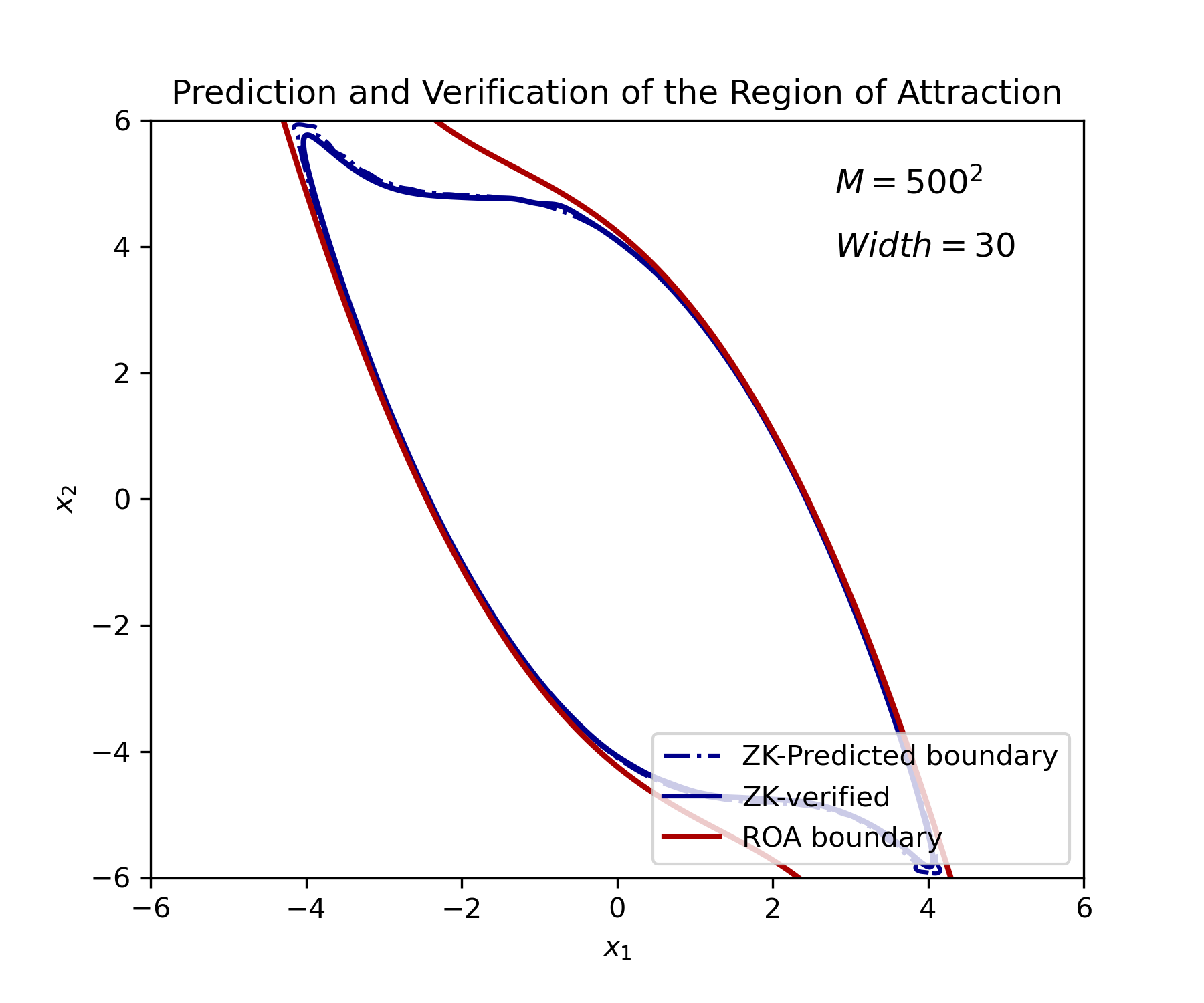
We use three experiments to investigate the effect of sample size and the width of the neural network: (1) , ; (2) , ; (3) , . In all of the experiments, we choose , , and for all . We use -layer NN model for the modification stage. The verified portion of the refined ROA are , and . Fig. 7 depicts the predicted and verified ROA with safety guarantees for the experiment (3). It can be seen that even though the actual ROA is unbounded, the proposed algorithm approximates the largest ROA that can be certified by the choice of neural Lyapunov function.
VII-D Stiff System I
In this example, we examine Van der Pol oscillators
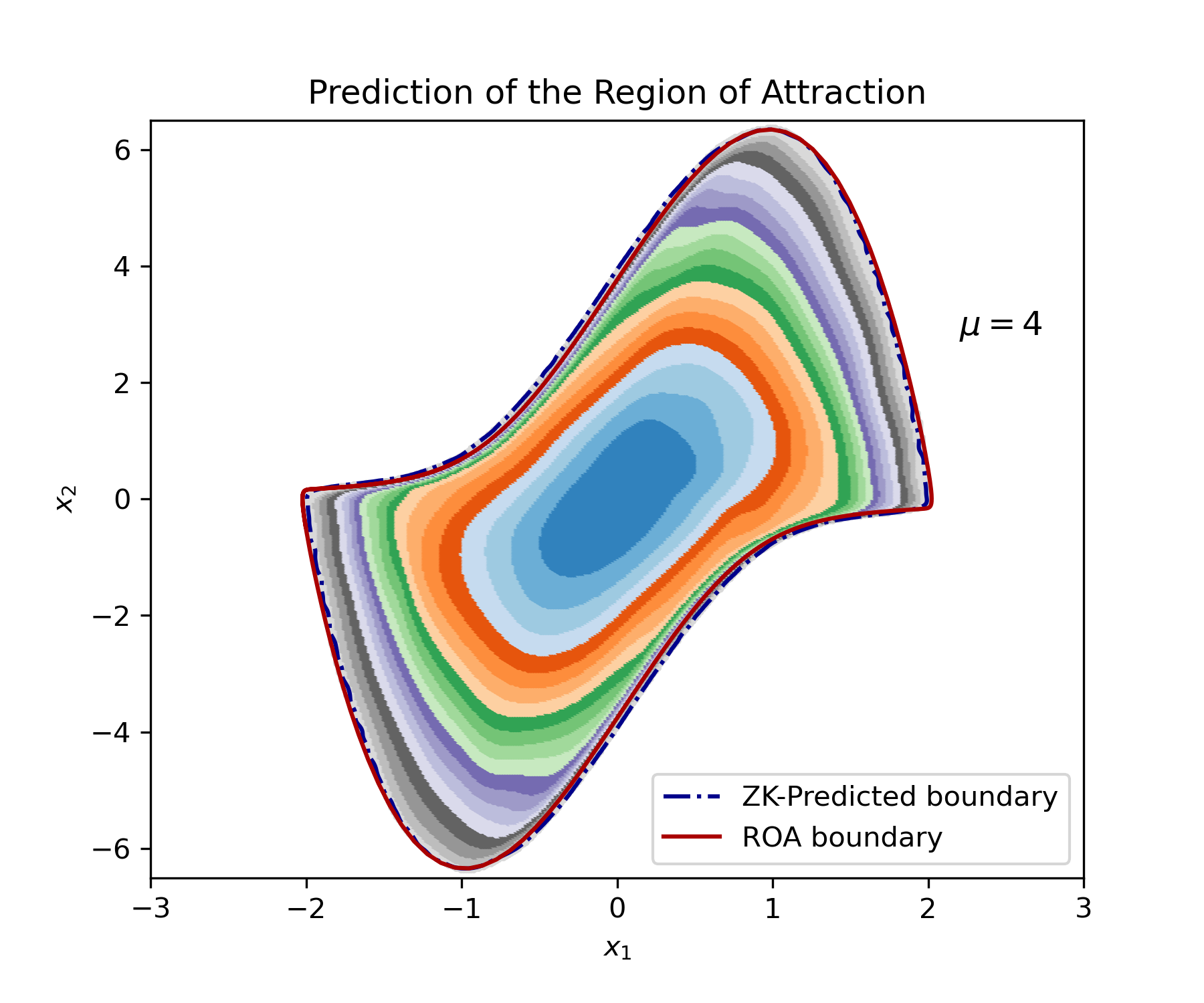
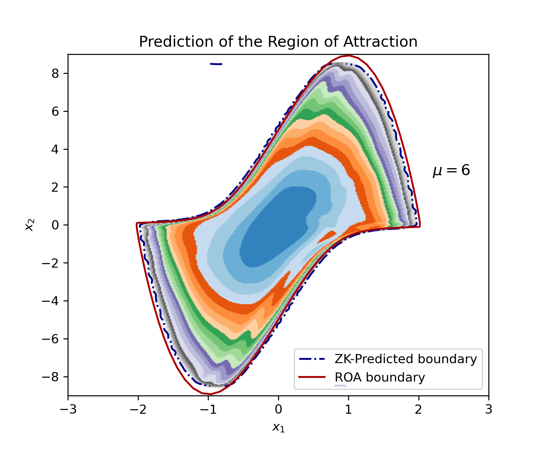
with and . The value of changes rapidly due to the high evolution speed of the state within the stiff systems. For both systems, we use samples to determine and employ a network model with two hidden layers and 15 neurons for modification. However, the rapid changes prevent the validation of a Lyapunov function. We present the color map of for predicting the ROAs in Fig. 8. We can observe that as increases, the same number of samples becomes insufficiently dense to provide adequate information for operator learning. This results in substantial oscillations at the boundaries of sub-level regions.
VII-E Stiff System II
We use this example to compare the predictability of ROA from [17, Example 3] for dynamics
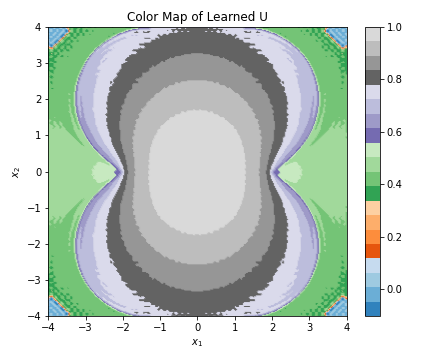
The origin is globally stable on . We choose and use samples to learn . The non-zero color map represents the ROA relative to , as shown in Fig. 9. The learned demonstrates better predictability than the local Lyapunov functions generated by conventional Koopman operators. We omit the NN-modification and formal verification in this example to make a fair comparison with [17].
VIII Conclusion
In this paper, we introduced a Zubov-Koopman approach to characterize the solution to Zubov’s equation, based on regularity and convergence analysis for a broader range of nonlinear systems. The proposed operator exhibits a semigroup property, and the learning technique is similar to the conventional Koopman operator. In particular, we executed an EDMD-like algorithm using a Fourier-like dictionary of observable functions based on our understanding of the solution properties. We then devise an iterative approach that employs the learned Zubov-Koopman operator to approximate the solution to Zubov’s equation, achieving a high level of accuracy. Compared to the existing data-driven methods, our proposed technique demonstrates a better predictability of the ROAs via numerical examples.
It is worth mentioning that, through numerical examples, we observed clear spectral gaps in the learned operators. This can potentially lead to dimension reduction for the Zubov-Koopman operators and effectively address the ‘curse of dimensionality’. Future directions will be on the spectral analysis with applications to high-dimensional physical systems.
One potential limitation of this work is its predictability of the flow in the state space. We have to rely on the knowledge of fixed points to predict the ROAs. It would be interesting to investigate how to align it with Koopman analysis so that the proposed method can be applied to situations with less information about the stable attractors.
Another immediate area for future work with the Zubov-Koopman framework could involve systems with robust control or other types of measurable inputs. It would be intriguing to explore its potential in predicting controllable regions with stability and safety properties for unknown systems.
Appendix A Fundamental Properties of Viscosity Solutions
We provide some fundamental properties of viscosity solutions in this appendix. The following lemma [28, Lemma 1.7, Lemma 1.8, Chapter I] provides some insights on and for some .
Lemma 38 (Sub- and Supperdifferential)
Let . Then
-
(1)
if and only if there exists such that and has a local maximum at ;
-
(2)
if and only if there exists such that and has a local minimum at ;
-
(3)
if for some both and are nonempty, then ;
-
(4)
the sets and are dense.
Appendix B Unique Bounded Viscosity Solutions
Proof of Theorem 19: The uniqueness property within follows the result [32, Thoerem 3.8] for zero perturbation of (1). Alternatively, we can suppose there exists another viscosity solution to with . Let . Then, solves with in a viscosity sense. One can follows a similar proof as in [28, Chapter II, Proposition 5.18] to show that for all and all . By the stability assumption, one has , which shows that is the unique viscosity solution on . For any valid , by the definition (13) and by [28, Chapter 2, Proposition 2.5], we immediately have that is the unique viscosity solution to (16) on .
Now we suppose . Then, . By the above uniqueness argument within , and by the construction of , all viscosity solutions to (16) should be equal to on . We then work on and verify that is the unique bounded viscosity solution to (16).
Let , then, . Suppose is another bounded viscosity solution to (16) and let for any . Then, . By the continuity of , there exists such that . Then, for any , . In addition, by the exact same argument as in [28, Chapter II, Theorem 3.1], one has that and as .
Now we argue that as , which will imply that on . If , then . If , then by the continuity of . If , set and . Then, is a local maximum for and is a local minimum for . Note that . In addition, since and are viscosity (sub/supper) solutions on , we have that and . This implies since . By the continuity of , we have as .
The other side, i.e., on , can be proved in the same manner. Therefore, on .
Appendix C Fundamental Properties of Zubov-Koopman
In the appendix, we complete the proof for Proposition 23.
Proof:
It is clear that . We also have the following identities.
which show the associativity of . The strong continuity of can be verified straightforwardly by Definition 2. For the second part of the proof, we apply dynamic programming and use the similar technique as above. We omit the details due to the similarity. ∎
References
- [1] Y. Li and J. Liu, “Robustly complete synthesis of memoryless controllers for nonlinear systems with reach-and-stay specifications,” IEEE Transactions on Automatic Control, vol. 66, no. 3, pp. 1199–1206, 2020.
- [2] F. Wilson, “Smoothing derivatives of functions and applications,” Transactions of the American Mathematical Society, vol. 139, pp. 413–428, 1969.
- [3] Y. Lin, E. D. Sontag, and Y. Wang, “A smooth converse lyapunov theorem for robust stability,” SIAM Journal on Control and Optimization, vol. 34, no. 1, pp. 124–160, 1996.
- [4] F. H. Clarke, Y. S. Ledyaev, and R. J. Stern, “Asymptotic stability and smooth lyapunov functions,” Journal of differential Equations, vol. 149, no. 1, pp. 69–114, 1998.
- [5] A. R. Teel and L. Praly, “A smooth lyapunov function from a class-estimate involving two positive semidefinite functions,” ESAIM: Control, Optimisation and Calculus of Variations, vol. 5, pp. 313–367, 2000.
- [6] A. Vannelli and M. Vidyasagar, “Maximal lyapunov functions and domains of attraction for autonomous nonlinear systems,” Automatica, vol. 21, no. 1, pp. 69–80, 1985.
- [7] K. K. Hassan et al., “Nonlinear systems,” Departement of Electrical and computer Engineering, Michigan State University, 2002.
- [8] P. Giesl and S. Hafstein, “Review on computational methods for Lyapunov functions,” Discrete & Continuous Dynamical Systems-B, vol. 20, no. 8, p. 2291, 2015.
- [9] C. Dawson, S. Gao, and C. Fan, “Safe control with learned certificates: A survey of neural Lyapunov, barrier, and contraction methods for robotics and control,” IEEE Transactions on Robotics, pp. 1–19, 2023.
- [10] S. L. Brunton, M. Budišić, E. Kaiser, and J. N. Kutz, “Modern koopman theory for dynamical systems,” arXiv preprint arXiv:2102.12086, 2021.
- [11] B. O. Koopman, “Hamiltonian systems and transformation in hilbert space,” Proceedings of the National Academy of Sciences, vol. 17, no. 5, pp. 315–318, 1931.
- [12] I. Mezić, “Spectral properties of dynamical systems, model reduction and decompositions,” Nonlinear Dynamics, vol. 41, pp. 309–325, 2005.
- [13] P. J. Schmid and J. Sesterhenn, “Dynamic mode decomposition of experimental data,” in 8th International Symposium on Particle Image Velocimetry, Melbourne, Victoria, Australia, 2009.
- [14] M. O. Williams, I. G. Kevrekidis, and C. W. Rowley, “A data–driven approximation of the koopman operator: Extending dynamic mode decomposition,” Journal of Nonlinear Science, vol. 25, pp. 1307–1346, 2015.
- [15] B. Lusch, J. N. Kutz, and S. L. Brunton, “Deep learning for universal linear embeddings of nonlinear dynamics,” Nature communications, vol. 9, no. 1, p. 4950, 2018.
- [16] O. Azencot, N. B. Erichson, V. Lin, and M. Mahoney, “Forecasting sequential data using consistent koopman autoencoders,” in International Conference on Machine Learning, pp. 475–485, PMLR, 2020.
- [17] A. Mauroy and I. Mezić, “A spectral operator-theoretic framework for global stability,” in 52nd IEEE Conference on Decision and Control, pp. 5234–5239, IEEE, 2013.
- [18] A. Mauroy and I. Mezić, “Global stability analysis using the eigenfunctions of the koopman operator,” IEEE Transactions on Automatic Control, vol. 61, no. 11, pp. 3356–3369, 2016.
- [19] S. A. Deka, A. M. Valle, and C. J. Tomlin, “Koopman-based neural lyapunov functions for general attractors,” in 2022 IEEE 61st Conference on Decision and Control (CDC), pp. 5123–5128, IEEE, 2022.
- [20] R. Zhou, T. Quartz, H. De Sterck, and J. Liu, “Neural lyapunov control of unknown nonlinear systems with stability guarantees,” Advances in Neural Information Processing Systems, vol. 35, pp. 29113–29125, 2022.
- [21] J. Liu, Y. Meng, M. Fitzsimmons, and R. Zhou, “Towards learning and verifying maximal neural lyapunov functions,” arXiv preprint arXiv:2304.07215, 2023.
- [22] L. Grüne, “Computing lyapunov functions using deep neural networks,” Journal of Computational Dynamics, vol. 8, no. 2, pp. 131–152, 2021.
- [23] M. Raissi, P. Perdikaris, and G. E. Karniadakis, “Physics-informed neural networks: A deep learning framework for solving forward and inverse problems involving nonlinear partial differential equations,” Journal of Computational physics, vol. 378, pp. 686–707, 2019.
- [24] W. Kang, K. Sun, and L. Xu, “Data-driven computational methods for the domain of attraction and zubov’s equation,” arXiv preprint arXiv:2112.14415, 2021.
- [25] Y. Lan and I. Mezić, “Linearization in the large of nonlinear systems and koopman operator spectrum,” Physica D: Nonlinear Phenomena, vol. 242, no. 1, pp. 42–53, 2013.
- [26] M. D. Kvalheim and S. Revzen, “Existence and uniqueness of global koopman eigenfunctions for stable fixed points and periodic orbits,” Physica D: Nonlinear Phenomena, vol. 425, p. 132959, 2021.
- [27] V. I. Zubov, Methods of AM Lyapunov and their application, vol. 4439. US Atomic Energy Commission, 1961.
- [28] M. Bardi, I. C. Dolcetta, et al., Optimal control and viscosity solutions of Hamilton-Jacobi-Bellman equations, vol. 12. Springer, 1997.
- [29] Q. J. Zhu, “Lower semicontinuous lyapunov functions and stability,” Journal of Nonlinear and Convex Analysis, vol. 4, p. 325, 2003.
- [30] M. Jones and M. M. Peet, “Converse lyapunov functions and converging inner approximations to maximal regions of attraction of nonlinear systems,” in 2021 60th IEEE Conference on Decision and Control (CDC), pp. 5312–5319, IEEE, 2021.
- [31] L. C. Evans, Partial Differential Equations, vol. 19. American Mathematical Society, 2010.
- [32] F. Camilli, L. Grüne, and F. Wirth, “A generalization of zubov’s method to perturbed systems,” SIAM Journal on Control and Optimization, vol. 40, no. 2, pp. 496–515, 2001.
- [33] Y. Meng, Y. Li, and J. Liu, “Control of nonlinear systems with reach-avoid-stay specifications: A lyapunov-barrier approach with an application to the moore-greizer model,” in 2021 American Control Conference (ACC), pp. 2284–2291, 2021.
- [34] Y. Meng, Y. Li, M. Fitzsimmons, and J. Liu, “Smooth converse lyapunov-barrier theorems for asymptotic stability with safety constraints and reach-avoid-stay specifications,” Automatica, vol. 144, p. 110478, 2022.
- [35] Y. Meng and J. Liu, “Lyapunov-barrier characterization of robust reach–avoid–stay specifications for hybrid systems,” Nonlinear Analysis: Hybrid Systems, vol. 49, p. 101340, 2023.
- [36] B. Oksendal, Stochastic differential equations: an introduction with applications. Springer Science & Business Media, 2013.
- [37] A. Mauroy and J. Goncalves, “Koopman-based lifting techniques for nonlinear systems identification,” IEEE Transactions on Automatic Control, vol. 65, no. 6, pp. 2550–2565, 2019.
- [38] G. Khromov and S. P. Singh, “Some fundamental aspects about lipschitz continuity of neural network functions,” arXiv preprint arXiv:2302.10886, 2023.