Exact solution and projection filters for open quantum systems subject to imperfect measurements
Abstract
In this paper, we consider an open quantum system undergoing imperfect and indirect measurement. For quantum non-demolition (QND) measurement, we show that the system evolves on an appropriately chosen manifold and we express the exact solution of the quantum filter equation in terms of the solution of a lower dimensional stochastic differential equation. In order to further reduce the dimension of the system under study, we consider the projection on the lower dimensional manifold originally introduced in [1] for the case of perfect measurements. An error analysis is performed to evaluate the precision of this approximate quantum filter, focusing on the case of QND measurement. Simulations suggest the efficiency of the proposed quantum projection filter, even in presence of a stabilizing feedback control which depends on the projection filter.
Index Terms:
Stochastic differential equation; Quantum projection filter; Open quantum systems; Quantum information geometry.I Introduction
Being able to reliably control quantum dynamics is a fundamental step towards the development of quantum technologies. Quantum systems may be assumed to be in closed or open form. Unlike closed systems, open quantum systems are by definition in interaction with an environment, hence they provide a more realistic description of physical systems. On the other hand, the interaction with the environment entails decoherence phenomena, characterized by a loss of information [2]. For controlled open quantum systems, closed-loop control strategies are preferable, compared to open-loop ones, due to robustness issues. A measurement-based feedback strategy can be realized based on an estimation of the state which is obtained by partial observations of the system. Such an estimation is called quantum filter or quantum trajectory in physics literature [3, 4, 5, 6]. The controlled dynamics obtained in this way fits in the framework of stochastic control, see e.g., [7] for further clarifications.
The works in e.g., [8, 9] present feedback stabilization of some particular open quantum systems by using geometric control, Lyapunov methods, and stochastic tools. Feedback stabilization methods are based on the real-time simulation of a quantum filter equation to obtain an estimate of the quantum state. The evolution of the quantum filter is usually described by a large number of equations and their simulation represents an obstacle to realize in real-time feedback strategies in real experiments. For instance, for a -qubit system, the evolution of the density matrix is described by stochastic differential equations. As in the classical case, in order to tackle this issue the basic idea is to seek reduced dynamics containing enough information in order to design efficient feedback controls based on them. Such feedback strategies should possibly be robust with respect to experimental imperfections. For instance, in [10], the authors show the robustness of a stabilizing feedback depending on a reduced dynamics only involving the diagonal elements of the filter state in the case of QND measurements.
The projection filtering strategy has been developed in the classical case in [11, 12, 13], based on differential and information geometry tools. To our knowledge, the quantum projection filter scheme was first proposed in [14]. Later, in [15] the authors obtained the evolution of system state in a lower dimensional manifold by unsupervised learning. This was achieved by use of local tangent space alignment. In [16], a dynamical law is derived by minimizing the statistical distance in the moving basis and an equivalence with the projection filter has been shown. Recently, in [1], a quantum projection filtering approach was developed in which the dynamics is projected onto a manifold consisting of an exponential family of unnormalized density matrices. An extended Kalman filter and numerical approaches have been respectively established in [17] and [18].
In this paper, we consider an open quantum system undergoing indirect measurement in presence of detection imperfections. Firstly by suitably choosing a submanifold of the state space, we show that the exact solution of the quantum filter equation under QND measurement can be expressed in parametrized form as where corresponds to the solution of a lower dimensional stochastic differential equation. Note that similar results have been derived for the particular case of qubit systems, with a different approach, in [19]. Then, in order to further reduce the complexity of the dynamics, i.e., to reduce the dimension of the parameter we follow the projection filter approach introduced in [1], originally developed for perfect measurements. Specifically we adapt the computation of the approximation error in the case of imperfect measurements. We observe that under QND measurements, the asymptotic behavior of the approximate projection filter is compatible with the original filter, in the sense that both dynamics converge to the set of invariant subspaces. This motivates the application of a projection filter in a stabilizing feedback control law. To this aim, we verify numerically the efficiency of the stabilizing feedback control introduced in [20] in the case of a two-level quantum system evaluated at the approximate filter. This is promising for further investigations.
This paper is organized as follows. Section II introduces the quantum filter equation under consideration. Section III is devoted to the study of its exact solution in the case of QND measurements. In Section IV, we develop the projection filter approach in the case of detection imperfections and we characterize the residual errors obtained from the projection process. We also derive a bound on the average total residual norm by assuming QND measurement. Also, we obtain a quantum state reduction result for the projection filter in the case of QND measurements. In Section V, we perform a numerical simulation for the case of a two-level system and discuss the application of the projection filter in the feedback design suggested in [20]. Section VI provides a summary and gives some future perspectives.
Notation. The singular values of matrix are denoted by . The commutator of matrices and is denoted by . A square matrix is said to be Hermitian if where corresponds to the complex conjugate transpose of The Frobenius norm of is defined by
II System description
Let us consider a finite dimensional open quantum system undergoing indirect measurement in the case of homodyne detection. The evolution of such a system is described by the following matrix-valued stochastic differential equation
| (1) |
The density operator belongs to the space of Hermitian, positive semidefinite operators of trace one acting on
In the above equation, is the Hamiltonian, represents the coupling operator, is the detector efficiency. The classical Wiener process is related to the observation process which is a continuous semimartingale with quadratic variation satisfying
| (2) |
Note that, for more general observation processes, the diffusion term in the evolution equation may be driven by a complex Wiener process (for more details see, e.g., [21]).
In the following we will mainly work with the Zakai equation, which is the unnormalized form of the quantum filter equation (1) and which is given by
| (3) |
In particular . Letting be the set of all Hermitian operators on the evolution corresponding to (3) takes place on the space
| (4) |
which is the closed subset of consisting of all nonnegative Hermitian operators on In particular can be seen as a differential manifold of dimension . We denote by , the tangent space of at the point , which is identified with .
Since the vector fields defining the dynamics are linear, hence globally Lipschitz, Equation (3) has a unique solution [22]. Since , we deduce that (1) has a unique solution as well.
For compatibility reasons with the differential manifold structure (see e.g. [12]), we further consider the Stratonovich form of the above equation, which is given by
| (5) |
where
III Exact Solution
In this section, under suitable assumptions, we construct a submanifold of such that the dynamics given by (5), with initial condition , is confined to and we express the dynamics in the corresponding coordinate system. In the following, we assume that is Hermitian, that is and that which corresponds to quantum non-demolition measurements [23]. In this case, we can write and , where the Hermitian operators are orthogonal projectors, that is and satisfying for every and and are positive integers. Without loss of generality, we assume and This is justified by the fact that replacing and by and respectively, does not affect the normalized dynamics given by (1).
Let and , with . Now define with
and
It can be easily verified that For the sake of simplicity, we assume that the set is linearly independent. Then is locally a -dimensional differential submanifold of , with tangent space given by
| (6) |
A direct calculation yields
| (7) |
| (8) |
| (9) |
We have the following lemma, which follows by direct calculation and by using (7), (8) and (9).
Lemma III.1.
The terms , and appearing in (5) belong to the tangent space Furthermore,
Now, we can establish the main result of this section.
Theorem III.2.
The solution of the quantum filter equation (1) with initial condition coincides with where with satisfying the stochastic differential equation
and
Proof.
By the previous lemma, the solutions of (5) evolve (almost surely) on and satisfy
| (10) |
On other hand, by the chain rule we have
| (11) |
To conclude, it is sufficient to identify the coefficients of the above equations with respect to the tangent space basis and solve the ordinary differential equations obtained for and ∎
IV Quantum projection filter and error analysis
IV-A The projection filter approach
The computation of the exact solution presented in Section III is valid under the assumption of quantum non-demolition measurements. In this section, we follow an approach called projection filter, see, e.g., [11, 14], which does not require the latter assumption and allows to further reduce the dimension of the system under study. This approach is mainly based on choosing an appropriate submanifold and suitably projecting the dynamics on it.
To formalize this approach, let us introduce some quantum information geometry tools, mainly borrowed from [1, 11].
Recall that , the tangent space of at the point may be identified with When a tangent vector is considered as an element of by this identification, we denote it by and we call it the -representation of .
We define a symmetrized inner product on as follows:
| (12) |
Next, the -representation of a tangent vector is defined as the Hermitian operator satisfying
| (13) |
By using (12) and (13) it is easy to obtain
| (14) |
Using the -representation defined above, a further inner product on is defined by
The quantum Fisher metric is a Riemannian metric whose components are
| (15) |
where and are given coordinates on .
Following [13, 1] (in the classical and quantum framework, respectively), we consider the subset of consisting of an exponential family of unnormalized quantum density operators
Here , is the initial condition for the (projected) dynamics, the operators , for , are assumed to be mutually commuting and pre-designed, and is an open subset of containing the origin. Assuming that the set {} is linearly independent, we obtain that is, locally, a -dimensional differential submanifold of . The tangent space at some is given by where Using (14) we get In analogy with (15) we define a Riemannian metric on whose components are real-valued functions of :
| (16) |
The matrix is a quantum Fisher information matrix. Then, for every , we can define an orthogonal projection operation by
| (17) |
where the are the components of the inverse of the quantum information
matrix .
We define the quantum projection filter on by
| (18) |
Since the vector fields regulating the dynamics are everywhere tangent to , the solution of the previous equation is a well-defined stochastic process on whenever belongs to Similarly to [1], by using the orthogonal projection operation and the chain rule
| (19) |
we can easily express the dynamics of the parameter as
| (20) |
with for . Here, the -th elements of the -dimensional column vectors and are
and Let be the normalized approximate quantum information state. We note that only SDEs need to be solved for instead of for the original quantum filter.
IV-B Error analysis
Following [13], we define at each point the prediction residual as and the two correction residuals as
respectively. These residuals refer to the local approximation errors due to the projection of the vector fields , and into the tangent space at time . For the sake of simplicity, we assume that the operator is Hermitian. This assumption simplifies the analysis of the local errors. By using the spectral theorem, we can write where is the number of nonzero distinct eigenvalues of denoted by and are orthogonal projections.
Let us set and We have the following result.
Proposition IV.1.
Assume and Then, the correction residuals are
and
Moreover, if , then the exponential quantum projection filter equation (20) becomes
| (21) |
and the prediction residual is given by
| (22) |
Proof.
Let denote the original probability measure under which is a Wiener process. By Girsanov theorem, there exists an equivalent probability measure such that in (2) becomes a Wiener process. Let denote the expectation with respect to the measure
To measure the gap between the filter state and its approximation, we consider the average total residual norm defined as
| (23) |
with . Also, set and We now state the main result of this section.
Theorem IV.2.
Let the assumptions of Proposition IV.1 hold true. If then
| (24) |
Proof.
Let us firstly note that . By using the triangular inequality, we get
Now, let We have
| (25) |
Define and . By using Lemma A.1 we get
| (26) |
where This comes from the fact that is a martingale with respect to
Under some additional conditions, Theorem IV.2 leads to an equivalence between the exponential quantum projection filter equation (18) and the quantum filter equation (3).
Corollary IV.3.
Let the assumptions of Proposition IV.1 hold true and assume in addition that Then
IV-C Quantum state reduction
Under the quantum non-demolition assumption , the normalized evolution of the quantum projection filter can be written as
| (28) |
where As in the previous section, let us write where is the number of nonzero distinct eigenvalues of denoted by and are orthogonal projections. The following result states that the quantum state reduction phenomenon occurs for both the evolutions given by (1) and by (28); it can be obtained by following standard stochastic LaSalle-type arguments similarly to [8], using the Lyapunov function .
Theorem IV.4.
Note that the previous result shows that the solutions of (1) and (28) share a similar asymptotic behavior, but it does not guarantee that such solutions converge almost surely to the same limit. The results obtained in [24, 10, 25] suggest that such limits coincide. It is then natural to expect that a feedback control depending on the quantum projection filter may be used to stabilize the system towards a chosen eigenstate of , similarly to what was done in, e.g., [8, 9].
V Numerical simulations
V-A A spin- system
Here we present simulation results for the simple case of a spin- system. For a two-level quantum system, can be uniquely characterized by the Bloch sphere coordinates as . The vector belongs to the ball We take and , where and are physical parameters.
It can be verified that the dynamics in the Bloch sphere coordinates are given by
| (29) |
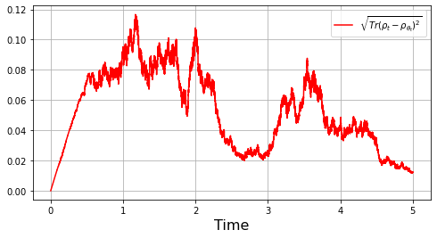
The operator can be written as where and and We note that is used to drive the exponential quantum projection filter. Here, the matrices , , and correspond to the Pauli matrices. We take with , and step size . Also, , , , , , and . The initial state is . Figure 1 shows the Frobenius norm of the difference between and .
V-B Discussion on the error in the presence of a feedback
Our goal is to study whether the approach developed in the previous sections remains effective in the presence of a controlled Hamiltonian. In particular, we wonder whether the quantum projection filter is a good candidate to replace the original filter in the stabilizing feedback law introduced in [20]. In that paper, the dynamics of a controlled spin- generalizing the dynamics (29) in presence of a control law takes the following form
In [20], a feedback controller is applied to stabilize the above system towards the excited state corresponding to the Bloch sphere coordinates The feedback takes the form
| (30) |
where , with and .
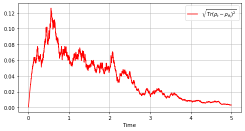
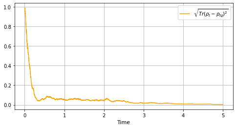
Here we assume that the feedback law (30) is evaluated at instead of and we study numerically the stabilization towards the excited state. The simulation parameters are the same as before. The validity of the proposed approximation filtering scheme is checked through the Frobenius norm of the difference between and in Figure 2. Figure 3 shows the convergence towards the target state.
VI Conclusions and Future works
In this paper we first develop an approach allowing us to derive the exact solution of the filter equation under QND measurement with imperfect measurements. Such a solution is described in terms of a solution of a simplified stochastic differential equation. To further reduce the complexity of the dynamics, we generalize the projection filter approach developed in [1] to the case of imperfect measurements. An analysis of the approximation error has been performed and a quantum state reduction result for the projected dynamics has been shown in the case of QND measurement. Simulations of a two-level system are provided with the aim of verifying the efficiency of the projection filtering method in the feedback stabilization design. In future work, we aim at improving the error estimate, for instance by making use of the approach established in [26], where a projection filter design for the case of perfect measurements was provided based on Stratonovich stochastic Taylor expansions. Further research lines include providing a rigorous analytic study for the stabilization property observed numerically and extending our results to the case .
Appendix
The following lemma collects some standard properties of singular values.
Lemma A.1. Let and be matrices. Then,
-
•
;
-
•
;
-
•
-
•
Acknowledgment
This work is supported by the Agence Nationale de la Recherche projects Q-COAST ANR- 19-CE48-0003 and IGNITION ANR-21-CE47- 0015I. The authors would like to thank Sofiane Chalal and Mario Neufcourt for the helpful discussions.
References
- [1] Q. Gao, G. Zhang, and I. R. Petersen, “An exponential quantum projection filter for open quantum systems,” Automatica, vol. 99, pp. 59–68, 2019.
- [2] E. B. Davies, Quantum theory of open systems. Academic Press, 1976.
- [3] V. P. Belavkin, “Nondemolition measurements, nonlinear filtering and dynamic programming of quantum stochastic processes,” in Modeling and Control of Systems. Springer, 1989, pp. 245–265.
- [4] L. Bouten, R. Van Handel, and M. R. James, “An introduction to quantum filtering,” SIAM Journal on Control and Optimization, vol. 46, no. 6, pp. 2199–2241, 2007.
- [5] A. Barchielli and M. Gregoratti, Quantum trajectories and measurements in continuous time: the diffusive case. Springer, 2009, vol. 782.
- [6] H. M. Wiseman and G. J. Milburn, Quantum measurement and control. Cambridge university press, 2009.
- [7] V. Belavkin, “Towards the theory of control in observable quantum systems,” arXiv preprint quant-ph/0408003, 2004.
- [8] M. Mirrahimi and R. Van Handel, “Stabilizing feedback controls for quantum systems,” SIAM Journal on Control and Optimization, vol. 46, no. 2, pp. 445–467, 2007.
- [9] W. Liang, N. H. Amini, and P. Mason, “On exponential stabilization of n-level quantum angular momentum systems,” SIAM Journal on Control and Optimization, vol. 57, no. 6, pp. 3939–3960, 2019.
- [10] W. Liang and N. H. Amini, “Model robustness for feedback stabilization of open quantum systems,” arXiv preprint arXiv:2205.01961, 2022.
- [11] S.-i. Amari and H. Nagaoka, Methods of information geometry. American Mathematical Soc., 2000, vol. 191.
- [12] D. Brigo, B. Hanzon, and F. LeGland, “A differential geometric approach to nonlinear filtering: the projection filter,” IEEE Transactions on Automatic Control, vol. 43, no. 2, pp. 247–252, 1998.
- [13] D. Brigo, B. Hanzon, and F. L. Gland, “Approximate nonlinear filtering by projection on exponential manifolds of densities,” Bernoulli, vol. 5, no. 3, pp. 495 – 534, 1999.
- [14] R. Van Handel and H. Mabuchi, “Quantum projection filter for a highly nonlinear model in cavity qed,” Journal of Optics B: Quantum and Semiclassical Optics, vol. 7, no. 10, p. S226, 2005.
- [15] A. E. Nielsen, A. S. Hopkins, and H. Mabuchi, “Quantum filter reduction for measurement-feedback control via unsupervised manifold learning,” New Journal of Physics, vol. 11, no. 10, p. 105043, 2009.
- [16] N. Tezak, N. H. Amini, and H. Mabuchi, “Low-dimensional manifolds for exact representation of open quantum systems,” Physical Review A, vol. 96, no. 6, p. 062113, 2017.
- [17] M. F. Emzir, M. J. Woolley, and I. R. Petersen, “A quantum extended kalman filter,” Journal of Physics A: Mathematical and Theoretical, vol. 50, no. 22, p. 225301, 2017.
- [18] P. Rouchon and J. F. Ralph, “Efficient quantum filtering for quantum feedback control,” Physical Review A, vol. 91, no. 1, p. 012118, 2015.
- [19] A. Sarlette and P. Rouchon, “Deterministic submanifolds and analytic solution of the quantum stochastic differential master equation describing a monitored qubit,” Journal of Mathematical Physics, vol. 58, no. 6, p. 062106, 2017.
- [20] W. Liang, N. H. Amini, and P. Mason, “On exponential stabilization of spin- systems,” in 2018 IEEE Conference on Decision and Control (CDC). IEEE, 2018, pp. 6602–6607.
- [21] H. Wiseman and A. Doherty, “Optimal unravellings for feedback control in linear quantum systems,” Physical Review Letters, vol. 94, no. 7, p. 070405, 2005.
- [22] P. E. Protter, Stochastic Integration and Differential equations. Springer, 2004.
- [23] V. B. Braginsky and F. Y. Khalili, Quantum measurement. Cambridge University Press, 1995.
- [24] W. Liang, N. H. Amini, and P. Mason, “Robust feedback stabilization of n-level quantum spin systems,” SIAM Journal on Control and Optimization, vol. 59, no. 1, pp. 669–692, 2021.
- [25] T. Benoist and C. Pellegrini, “Large time behavior and convergence rate for quantum filters under standard non demolition conditions,” Communications in Mathematical Physics, vol. 331, no. 2, pp. 703–723, 2014.
- [26] Q. Gao, G. Zhang, and I. R. Petersen, “An improved quantum projection filter,” Automatica, vol. 112, p. 108716, 2020.