Circuit realisation of a two-orbital non-Hermitian tight-binding chain

Abstract

We examine a non-Hermitian (NH) tight-binding system comprising of two orbitals per unit cell and their electrical circuit analogues. We distinguish the $\mathcal{PT}$-symmetric and non-$\mathcal{PT}$ symmetric cases characterised by non-reciprocal nearest neighbour couplings and onsite gain/loss terms, respectively. The localisation of the edge modes or the emergence of the topological properties are determined via the maximum inverse participation ratio, which has distinct dependencies on the parameters that define the Hamiltonian. None of the above scenarios exhibits the non-Hermitian skin effect. We investigate the boundary modes corresponding to the topological phases in a suitably designed electrical circuit by analyzing the two-port impedance and retrieve the admittance band structure of the circuit via imposing periodic boundary conditions. The obtained results are benchmarked against the Hermitian version of the two-orbital model to compare and discriminate against those obtained for the NH variants.

I Introduction

The mathematical discipline of topology, dedicated to the investigation of geometric properties preserved under continuous transformations, has witnessed a remarkable convergence with the field of condensed matter physics in the past few decades. The seminal proposal of topological states in polyacetylene chain [1] and the presence of quantised edge modes in the quantum Hall effect [2] marked pivotal turning discoveries, highlighting the role of topology in characterising novel phases of matter. Thus, a prominent subset of materials, known as ‘topological insulators’, has emerged as a central focus in contemporary research due to their unique electronic properties, particularly the presence of gapless edge modes that persist even under alteration of the band properties as long as the spectral gap stays open [3, 4, 5]. At the core of this inquiry lies the classification of distinct phases based on the underlying symmetries of the system, such as time-reversal symmetry (TRS), particle-hole symmetry (PHS), and chiral symmetry (CS). The culmination of these efforts has led to the establishment of a comprehensive classification scheme for the topological insulators, commonly referred to as the ‘ten-fold’ way [6, 7].

Although we are trained to think about Hermitian systems with the energy being observable, and always assuming real values, there is significant enthusiasm for non-Hermitian (NH) systems as well. Building upon foundational work by Bender and Boettcher [8], it has been demonstrated that NH systems, exhibiting parity and time-reversal ($\mathcal{PT}$) symmetry may manifest real eigenspectra, despite the shift from the Hermitian paradigm. The parity operator ($\mathcal{P}$) acts on the spatial part of a given state, resulting in an inversion of the position, whereas the time-reversal operator ($\mathcal{T}$) reverses the dynamical part, changing the sign of the momentum. In particular, the interplay of the topology and NH systems [9, 10] has emerged as a captivating frontier in the realm of condensed matter physics. Particularly, the ‘ten-fold way’ is upgraded to a $38$-fold classification scheme [11]. This fortuitous interplay has unveiled an array of fascinating physical phenomena, notably including the non-Hermitian skin effect (NHSE), wherein eigenstates predominantly localise near the system boundaries and display pronounced sensitivity to boundary conditions [12, 13, 14, 15, 16, 17]. Consequently, the conventional concept of the Brillouin zone is challenged by the non-Bloch theory [18, 19], introducing a generalised Brillouin zone approach. Exceptional points [13, 21, 22], where the eigenvalues and eigenfunctions of the ‘defective’ Hamiltonian coalesce, have emerged as fundamental features in studying NH systems. Thus, NH systems present a vast platform to explore the connection between topology and non-Hermiticity. The experimental exploration of these kinds of systems has been materialised in diverse physical settings, spanning ultra-cold atoms in optical lattices [23, 24], electronic [25, 26, 27], mechanical [28], and acoustic [29, 30] systems. Remarkably, electrical circuits have surfaced as a versatile platform for investigating the topological properties, owing to the inherent simplicity and adaptability in circuit design [31, 32, 33, 34, 35, 36, 37, 38, 39, 40]. Comprising of the fundamental electronic components, these circuits yield outcomes exclusively contingent upon the connectivity, quite unlike the conventional knowledge based upon the Bravais vectors or lattice constants in tight binding (TB) systems. As a result, these readily accessible and cost-effective electrical circuits provide a convenient and effective technique for experimental verification of quantum systems.

Our investigation centres around a comprehensive exploration of the intricate relationship between topology and NH systems through a one-dimensional TB system comprising of two orbitals, $s$ and $p_{x}$, and their implementation in electronic circuits. Additionally, we explore NH variants of the traditional (Hermitian) system, characterised by the presence (or absence) of $\mathcal{PT}$ symmetry. The NH models are introduced through onsite gain/loss terms and non-reciprocal coupling strengths, leading to a detailed examination of their localisation and spectral behaviour, respectively, under open boundary condition (OBC) and periodic boundary condition (PBC). Section II presents our results in a systematic sequence. To summarise, we explore the properties of three TB models. We begin with an in-depth discussion of the Hermitian case, followed by thoroughly exploring the non-$\mathcal{PT}$ symmetric and $\mathcal{PT}$ symmetric cases. This sequential approach provides a clear understanding of the distinct behaviours exhibited by each of the above scenarios. Subsequently, we delve into a comprehensive topoelectrical analysis of each of the TB models. This involves the construction of electronic circuits and simulating their observational properties, like impedance profiles and admittance band structures (ABS), providing a bridge between theoretical models and experimental setups. In section III, we summarise the results.

II Models and Results

II.1 Hermitian circuit

We begin by considering a straightforward yet inclusive Hermitian ladder-type lattice model, where each unit cell accommodates a solitary atom endowed with a pair of orbitals—specifically, the $s$ and the $p_{x}$ orbitals. The model’s Hamiltonian is expressed as follows:

$$H_{1}=\sum_{i=1}^{L} \bigg{[}\epsilon(\hat{s}_{i}^{\dagger}\hat{s}_{i}-\hat{p}_{i}^{\dagger}\hat{p}_{i})-t_{ps}\hat{s}_{i}^{\dagger}\hat{p}_{i-1}\bigg{]}+$$

$$\sum_{i=1}^{L-1}\bigg{[}-t(\hat{s}_{i}^{\dagger}\hat{s}_{i+1}-\hat{p}_{i}^{\dagger}\hat{p}_{i+1})+t_{ps}\hat{s}_{i}^{\dagger}\hat{p}_{i+1}\bigg{]}+\textrm{H.c.}$$ (1)

Here, $\pm\epsilon$ symbolises the onsite potentials pertaining to the $s$ and $p_{x}$ orbitals, respectively. The hopping strengths are denoted by $-t$ ($t$) and $t_{ps}$ ($-t_{ps}$), governing the inter-cellular transitions $s^{i-1}\leftrightarrow s^{i}$ ($p_{x}^{i-1}\leftrightarrow p_{x}^{i}$) and $s^{i-1}\leftrightarrow p_{x}^{i}$ ($p_{x}^{i-1}\leftrightarrow s^{i}$), correspondingly. $s^{i}$ and $p_{x}^{i}$ refer to the $s$ and $p_{x}$ orbitals at the $i^{th}$ unit cell, and $L$ denotes the system size or equivalently, the total count of unit cells. The operators $\hat{s}_{i}$ ($\hat{s}_{i}^{\dagger}$) and $\hat{p}_{i}$ ($\hat{p}_{i}^{\dagger}$) denote the annihilation (creation) operators for spinless fermions that pertain to the $s$ and $p_{x}$ orbitals, respectively, at the $i^{th}$ unit cell. The intra-orbital hopping term (between $s$ and $p_{x}$ orbitals within the same unit cell) is ignored. In the context of PBC, the Hamiltonian in Eq.(1) can be stated in the ensuing Bloch form as,

$$h_{1}(k)=\begin{pmatrix}\epsilon-2t\cos k&2it_{ps}\sin k\\ -2it_{ps}\sin k&-\epsilon+2t\cos k\end{pmatrix}.$$ (2)

In the present case, the system has TRS, which is given by the following relation for any $h(k)$ [7],

$$\mathcal{T}h(k)\mathcal{T}^{-1}=h(-k);\quad\mathrm{with}\quad\mathcal{T}^{2}=\pm 1,$$

where $\mathcal{T}$ ($=U_{T}\mathcal{K}$, $U_{T}$ being a unitary matrix) is the TRS operator that is anti-unitary in nature, and $h_{1}(k)$ satisfies the above equation. For systems consisting of spinless fermions (present case), $\mathcal{T}$ is nothing but the complex conjugation operator $\mathcal{K}$ and $\mathcal{T}^{2}=1$. In the same way, the system also possesses PHS, which is written as,

$$\mathcal{C}h(k)\mathcal{C}^{-1}=-h(-k);\quad\mathrm{with}\quad\mathcal{C}^{2}=\pm 1.$$

The anti-unitary PHS operator $\mathcal{C}=U_{C}\mathcal{K}$ ($U_{C}$ is unitary) anti-commutes with the Bloch Hamiltonian $h_{1}(k)$, where $U_{C}=\sigma_{x}$ for the present case. Evidently, the chiral symmetry (CS) is also there since the CS operator ($\Gamma$) is nothing but $\Gamma=\mathcal{T}\cdot\mathcal{C}$. These properties allow us to conclude that the system falls in the class $\boldsymbol{\mathrm{BDI}}$ in $\boldsymbol{\mathrm{AZ}}$ symmetry class.

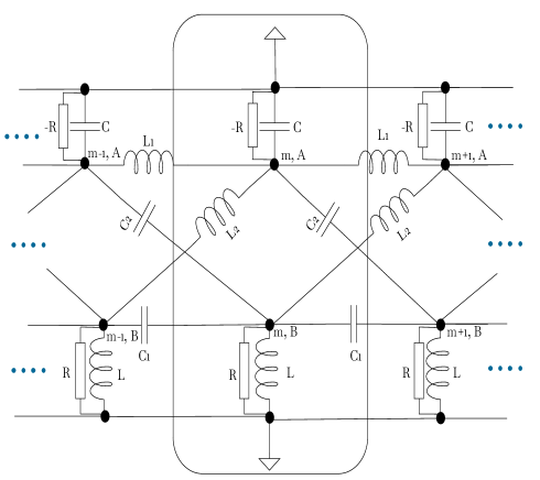
Figure 1: Hermitian circuit diagram for $3$ subsequent unit cells, denoted by $m$ and sublattices $A\;\mathrm{and}\;B$, are depicted here. The rectangular box represents a unit cell. The black dots represent all the connections. For the present case, $|R|=\infty$ implies that the connection is disjunctive there. The expressions (and values) of all the remaining circuit elements are given in the text.

Hence, we then proceed to construct an electrical circuit whose Laplacian [41] bears a striking resemblance to the Hamiltonian presented in Eq.(1). This endeavour is accomplished by strategically integrating inductors and capacitors, as shown in Fig.1. For an electrical network, $\mathcal{L}$, consisting of $N$ nodes, if $J$ denotes the Laplacian and $V_{a}$ and $I_{a}$ denote the voltage and the current flowing into node ‘$a$’ from the source placed elsewhere respectively, then the following relation must hold,

$$I_{a}=\sum_{b(a\neq b)}C_{ab}(V_{a}-V_{b})+C_{a}V_{a}\quad\mathrm{for}\quad a=1,2,3....N,$$ (3)

where $C_{ab}$ is the conductance between two distinct nodes $a$ and $b$. Note that the term $C_{aa}$ bears no meaning and can be put to zero, whereas $C_{a}$ is the resultant conductance between node $a$ and the ground. Thus, Eq.(3) reads $I=JV$, where $J$, $V$ and $I$ denote the Laplacian, the voltage and the current profile of the circuit, respectively. Consequently, the elements of the Laplacian matrix will be,

$$J_{ab}=C_{ab}+\delta_{ab}W_{a},\quad\mathrm{where}\quad W_{a}=\sum_{b}C_{ab}+C_{a}.$$

Now, one of the measurable quantities for the circuit is the impedance between two nodes, namely $a$ and $b$, which is given by,

$$Z_{ab}=\sum_{j_{n}\neq 0}\frac{|\psi_{n,a}-\psi_{n,b}|^{2}}{j_{n}},$$ (4)

where $j_{n}$ is the $n^{\mathrm{th}}$ eigenvalue of the Laplacian $J$ and $\psi_{n,a}$ is the $a^{\mathrm{th}}$ element of the corresponding eigenmode.

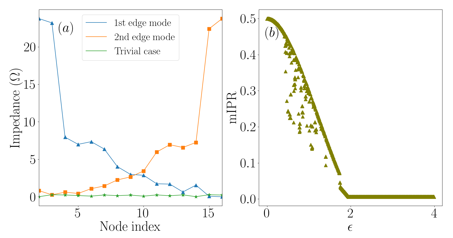
Figure 2: (a) The impedance profile (IP) of the Hermitian circuit, comprising eight unit cells, for both the trivial and the topological cases. The first port is fixed at the first and last nodes to obtain the second and first edge modes. We have kept the values of $C_{1}$, $L_{1}$, $C_{3}$ and $L_{3}$ fixed at $22\;\mu F$, $27\;\mu H$, $6.8\;\mu F$ and $87\;\mu H$, respectively. The resonating frequency of the circuit is $f\approx 6.53\;kHz$. For the trivial case ($C_{2}+C_{3}<3C_{1}$), we have kept the values of $C_{2}$ and $L_{2}$ fixed at $68\;\mu F$ and $8.7\;\mu H$, while for topological case ($C_{2}+C_{3}>3C_{1}$), those have values $33\;\mu F$ and $18\;\mu H$ respectively. (b) mIPR vs $\epsilon$ is shown for the Hermitian TB model comprising $250$ unit cells. The plot suggests that the edge states are non-existent after the point $\epsilon=2t$. Here we have set $t=t_{ps}=1$ and set the energy scale to be in a unit of $t$.

Returning to the construction of a suitable circuit, the hopping parameters $t$ ($-t$) and $t_{ps}$ ($-t_{ps}$) of the TB model are embodied by the capacitors (and inductors) denoted as $C_{1}$ (and $L_{1}$) and $C_{2}$ (and $L_{2}$), as shown in Fig.1. Furthermore, the modulation of the onsite potential, denoted by $\pm\epsilon$, is deftly achieved by utilising elements $C_{3}$ and $L_{3}$. Note that the circuit elements $C$ (and $L$), which are connected to the ground, are parallel combinations of $C_{1}$, $C_{2}$ and $C_{3}$ (and $L_{1}$, $L_{2}$ and $L_{3}$), respectively, which yields $C=C_{1}+C_{2}+C_{3}$ $\left(\mathrm{and}\;\frac{1}{L}=\frac{1}{L_{1}}+\frac{1}{L_{2}}+\frac{1}{L_{3}}\right)$. The topological properties of the TB model shall manifest through the emergence of the robust zero-energy boundary modes in real space. Crucially, the Laplacian, $J$, reveals the topological boundary resonances (TBR) at a resonating angular frequency $\omega_{0}$, defined via,

$$\omega_{0}=\frac{1}{\sqrt{L_{1}C_{1}}}=\frac{1}{\sqrt{L_{2}C_{2}}}=\frac{1}{\sqrt{L_{3}C_{3}}}$$

provided that our circuit, mirroring the associated TB model, resides in the topological phase. A topological phase transition, that is, an emergence of a trivial phase in our circuit, manifests at the critical condition $C_{2}+C_{3}=3C_{1}$. This corresponds to a spectral gap-closing scenario that occurs for the TB model.

Our quest for deeper insights into the electrical circuits and their relevance to topological phenomena leads us to calculate the two-port impedance, in which one port remains anchored at the edge of the circuit while the other is systematically connected to each node within the network. Consequently, we obtain impedance measurements corresponding to each node, as demonstrated in Fig.2(a). Notably, the impedance profile (IP) observed corresponding to the topological scenario, wherein $C_{2}+C_{3}<3C_{1}$, remarkably mirrors the exponentially decaying probability distribution associated with the zero-energy edge modes. Within the trivial regime, the entire profile hovers near zero, indicating that the corresponding eigenmode in the TB model extends uniformly across all the sites.

Now, let us look at the TB model corresponding to OBC. To establish the localisation characteristics of the eigenstates, we employ a well-known approach involving computation of the inverse participation ratio (IPR) [43] for the TB model, defined via,

$$\mathrm{IPR}^{(i)}=\frac{\sum_{n}|\psi^{i}_{n}|^{4}}{\left(\sum_{n}|\psi^{i}_{n}|^{2}\right)^{2}},$$ (5)

where $\mathrm{IPR}^{(i)}$ represents the IPR associated with the $i$-th eigenstate, while $n$ signifies the site index. It is firmly established that for extended states, the IPR exhibits an inverse relationship with the system size ($\sim L^{-1}$), which tends to zero for sufficiently large system sizes.

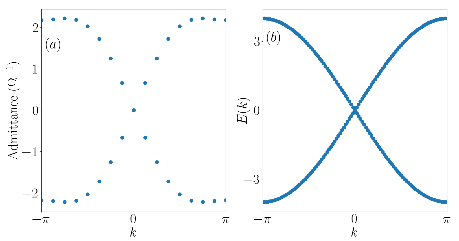
Figure 3: (a) The ABS of the Hermitian ladder circuit with eight unit cells, as described by Eq.(6). The values of circuit elements are the same as for the circuit with OBC, except for $C_{1}$ and $L_{1}$, taking the values $13.3\mu F$ and $44.6\mu H$, respectively. (b) The band structure of the corresponding TB model, comprising of $50$ unit cells, is shown at the phase transition point ($\epsilon=2t$). It correctly replicates the ABS, shown in (a).

In contrast, the IPR remains a constant for localised states and is insensitive to the system size. Further, it approaches unity in the thermodynamic limit where the states are entirely confined to individual sites. Here, we calculate the ”maximum IPR” (mIPR), which denotes the IPR of the edge states in the topological phase and also refers to the highest IPR value among all the eigenstates corresponding to the trivial phase. The plot of mIPR against $\epsilon$, given in Fig.2(b), denotes that the boundary modes exist for $\epsilon<2t$ ($t=1$ in our work) and hence imposes the condition for the topological phase transition to occur at $\epsilon=2t$, a profound equivalence to the identity $C_{2}+C_{3}=3C_{1}$ as predicted by the circuit Laplacian. This equivalence can be understood as the TB potential $\epsilon$ is expressed via $\epsilon\equiv C_{2}+C_{3}-C_{1}$ and $t\equiv C_{1}$ as mentioned before.

If we consider PBC in the circuit, a Fourier transformation of the Laplacian introduces a wave number component ‘$k$’ per unit cell and spawns a 2x2 constitutive block matrix,

$$J_{H}(\omega,k)=\begin{pmatrix}\frac{1}{i\omega L_{1}}+i\omega(C_{2}+C_{3})+\frac{2}{i\omega L_{1}}\cos k&-2\omega C_{2}\sin k\\ \frac{2}{\omega L_{2}}\sin k&i\omega C_{1}+\frac{1}{i\omega L_{2}}+\frac{1}{i\omega L_{3}}+2i\omega C_{1}\cos k\end{pmatrix}.$$ (6)

In the absence of any dissipative losses, the spectrum manifests a purely imaginary form; however, in the presence of dissipation, it takes on a complex character. Upon imposing the PBC on the circuit, the number of certain ‘significant’ nodes decreases, aligning with the number of sublattices within a unit cell, for example, two in this case. So, we need only to introduce an input current into two distinct sublattices and measure the voltage responses of the circuit [31]. Subsequently, we express these responses in terms of Fourier modes, assuming translational invariance of the system. The combined result from the above scenarios gives rise to an admittance spectrum, as presented through Eq.(6), and the results are prominently illustrated in Fig.3(a). The ABS profile is symmetric with respect to the value $0$, suggesting that the circuit is chirally symmetric.

Meanwhile, the band structure of the TB model takes the form $E_{1\pm}(k)=\pm\sqrt{(-\epsilon+2t\cos k)^{2}+4t_{ps}^{2}\sin^{2}k}$ as obtained from Eq.(2), and presented in Fig.3(b). It is imperative to acknowledge that the parameter values employed herein accurately determine the specific location where the topological phase transition occurs. Consequently, this distinctive choice of parameters reveals a gap closure phenomenon at $k=0$. Thus, it denotes a critical point in our analysis.

II.2 non-$\mathcal{PT}$ symmetric NH circuit

In this section, we engineer an NH lattice model by introducing a staggered imaginary onsite potential term to the two orbitals. This modification substitutes $\epsilon$ with $i\epsilon$ in Eq.(1) for OBC. This particular form of potential within the Hamiltonian signifies a dynamic exchange of energy, encompassing both ”gain” and ”loss”, a direct consequence of the non-Hermiticity. The inclusion of the $i\epsilon$ term disrupts the TRS of the system, rendering it devoid of the $\mathcal{PT}$ or anti-$\mathcal{PT}$ symmetry, mandating that the eigenspectra of the system to assume on a complex nature. In the realm of the $k$ space, the corresponding Bloch Hamiltonian is elegantly expressed as follows:

$$h_{2}(k)=\begin{pmatrix}i\epsilon-2t\cos k&2it_{ps}\sin k\\ -2it_{ps}\sin k&-i\epsilon+2t\cos k\end{pmatrix},$$ (7)

which yields the expression for the band structure as,

$$E_{2\pm}(k)=\pm\sqrt{(-i\epsilon+2t\cos k)^{2}+4t_{ps}^{2}\sin^{2}k}.$$ (8)

The creation of an analogous electric circuit is accomplished by incorporating both positive and negative resistive components, $\pm R$ [35, 42], strategically connected between the circuit nodes and the reference ground, as illustrated in Fig.1. Furthermore, we have set $C=2C_{1}$ and $L=\frac{L_{1}}{2}$ to cancel out any additional terms in the onsite potential other than $\pm R$. This makes the scenario completely equivalent to $\pm i\epsilon$ in the corresponding TB model. It is important to note that the implementation of negative impedance is accomplished through negative impedance converters with current inversion, known as INIC. It works on the principle of the negative feedback configuration of an OP-amp. A comprehensive discussion and guidelines for using the INICs have been covered in some of the earlier works [35, 38, 42].

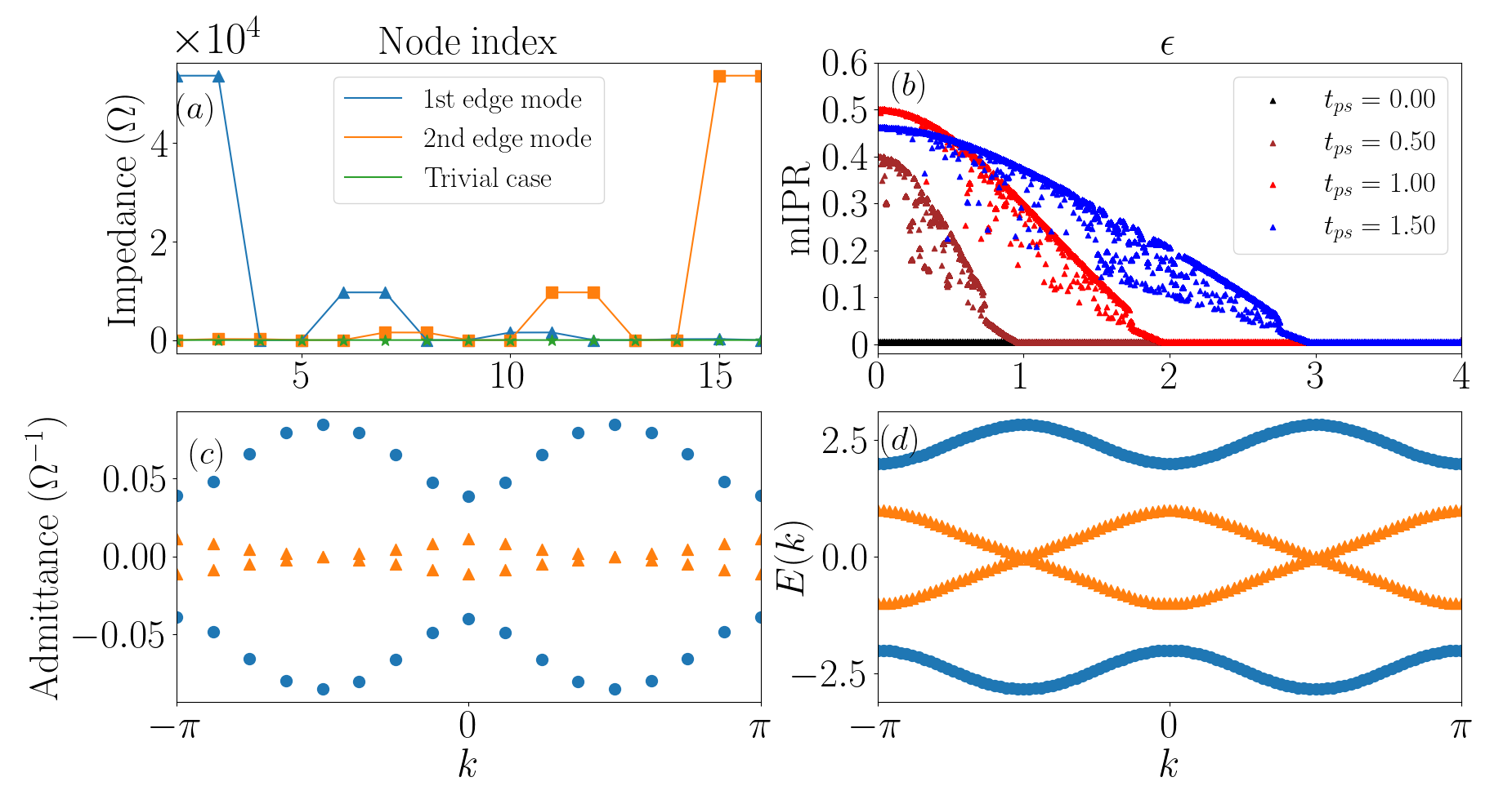
Figure 4: (a) The IP of the non-$\mathcal{PT}$ symmetric NH circuit, constituting of eight unit cells. The trivial and the topological cases correspond to the values of $R$ being $10\;\Omega$ and $100\;\Omega$, respectively. (b) mIPR (defined in the text) versus $\epsilon$ is plotted here for different values of $t_{ps}$ keeping $t=1$. The plot suggests that the existence of the edge states now depends on $t_{ps}$, unlike the Hermitian model, which depends on $t$. The real and imaginary parts of (c) the ABS and (d) the band structure of the corresponding TB model are represented by the circles and triangles, respectively.

In Fig.4(a), we present the IP for the non-$\mathcal{PT}$ symmetric NH circuit, which has been achieved within both the trivial and topological regions employing the method expounded in the previous section. To aid the comprehensibility of our results, we have maintained the values of the circuit components identical to that of the Hermitian case, except that the capacitors have been scaled down to the nanofarad ($nF$) range. Such rescaling allows us a better demonstration of our results on IP and ABS. Thus, the resonant frequency of the circuit has an approximate value, $f=\frac{\omega_{0}}{2\pi}\approx 206.5\;kHz$. The criterion for the topological phase transition in this scenario is succinctly expressed as $R=\frac{1}{2\omega_{0}C_{2}}\approx 11.68\;\Omega$. Fig.4(b) showcases the variation of mIPR against $\epsilon$ for four distinct values of $t_{ps}$, namely, $t_{ps}=0,0.5,1\;\mathrm{and}\;1.5$. These results validate the notion that the phase transition critically hinges upon the interplay between $\epsilon$ and $t_{ps}$, which is analogous to the condition, $R=\frac{1}{2\omega_{0}C_{2}}$, for the circuit. Consequently, mIPR exhibits non-zero values for $\epsilon<2t_{ps}$, transitioning to zero for $\epsilon>2t_{ps}$, thereby signifying the topological and trivial regions, respectively. It is pertinent to mention that the calculation of mIPR follows the same formula as presented in Eq.(5), albeit with the introduction of the right eigenvectors [20] tailored to this specific case.

For PBC, the Laplacian can be written in Bloch form in the reciprocal space as,

$$J_{NH_{1}}(\omega,k)=\left[\left(\frac{i}{R}+\frac{2}{i\omega L_{1}}\cos k\right)\sigma_{z}+\frac{2}{i\omega L_{2}}\sin k\;\sigma_{y}\right],$$ (9)

where $\sigma_{i}$ is the i-th $(2\times 2)$ Pauli matrix. The inclusion of the resistive element $R$ introduces energy dissipation within the circuit, resulting in a complex admittance profile. Fig.4(c) provides a comprehensive visualisation of the real and imaginary parts of the ABS as a function of the momentum $k$. Key parameters for this representation include values of $C_{1}$, $L_{1}$, and $R$ set at $15\;\mu F$, $39\;\mu H$, and $100\;\Omega$, respectively, while keeping the other parameters consistent with those employed in Fig.4(a). Remarkably, the admittance spectra exhibit a transition into a real domain at the points $k=\pm\frac{\pi}{2}$. This transformation occurs due to the topological phase that the system resides in. Consequently, this behaviour faithfully replicates the band structure of the non-$\mathcal{PT}$ symmetric model, as encapsulated by Eq.(8) and depicted in Fig.4(d). Conducting a spectral analysis of this model reveals the presence of a line gap, a crucial characteristic that substantiates the absence of NHSE [16]. This, in turn, ensures the validation of the bulk-boundary correspondence (BBC).

II.3 $\mathcal{PT}$-symmetric NH circuit

Now, we take recourse to break the Hermiticity of $H_{1}$ by including a non-reciprocity parameter, $\delta$, in the hopping term among the $s$ and $p_{x}$ orbitals ($t_{ps}$) from neighbouring unit cells. The new Hamiltonian in OBC takes the form,

$$H_{3}=H_{1}+\delta\left[\sum_{i=1}^{L-1}(\hat{s}_{i}^{\dagger}\hat{p}_{i+1}-\hat{p}_{i+1}^{\dagger}\hat{s}_{i})-\sum_{i=2}^{L}(\hat{s}_{i}^{\dagger}\hat{p}_{i-1}-\hat{p}_{i-1}^{\dagger}\hat{s}_{i})\right]$$ (10)

with the Bloch Hamiltonian, $h_{3}(k)$, given by,

$$h_{3}(k)=\begin{pmatrix}\epsilon-2t\cos k&2i(t_{ps}+\delta)\sin k\\ -2i(t_{ps}-\delta)\sin k&-\epsilon+2t\cos k\end{pmatrix}.$$ (11)

which indicates that the forward ($s^{i}\rightarrow p_{x}^{i+1}$) and the backward ($s^{i}\leftarrow p_{x}^{i+1}$) hopping amplitudes between $s^{i}$ and $p_{x}^{i+1}$ is $t_{ps}-\delta$ and $t_{ps}+\delta$, respectively.

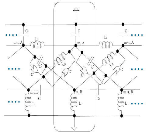
Figure 5: Circuit diagram for $\mathcal{PT}$-symmetric circuit. The INICs are denoted by the arrowheads, which offer an impedance $C^{\prime}=C_{x}$ and $C^{\prime}=-C_{x}$ for the forward ($m-1,\;A/B\rightarrow m,\;B/A$) and backward ($m,\;A/B\rightarrow m-1,\;B/A$) direction of current, respectively. Thus, the conductance between the nodes becomes $i\omega(C_{2}\pm C_{x})$ from the directional point of view. The expressions (or values) for the remaining circuit elements are given in the text.

The non-reciprocity term does not affect the TRS. To establish $\mathcal{PT}$ symmetry, we shall perform a unitary transformation on $h_{3}(k)$. This is achieved via a unitary matrix $U$, such that,

$$h_{3}^{\prime}(k)=U^{\dagger}h_{3}(k)U;\quad\mathrm{where}$$

$$U=\frac{1}{\sqrt{2}}\begin{pmatrix}1&-1\\ 1&1\end{pmatrix},$$ (12)

which yields,

$$h^{\prime}_{3}(k)=\begin{pmatrix}2i\delta\sin k&-\epsilon+2t\cos k+2it_{ps}\sin k\\ -\epsilon+2t\cos k-2it_{ps}\sin k&-2i\delta\sin k\end{pmatrix},$$ (13)

It is evident that $h^{\prime}_{3}(k)$ commutes with the $\mathcal{PT}$ operator, defined as $\sigma_{x}\mathcal{K}$, where $\mathcal{K}$ represents the complex conjugation operator. This commutation implies the preservation of $\mathcal{PT}$ symmetry. Subsequently, $h_{3}(k)$ and $h_{3}^{\prime}(k)$ are connected via a similarity transformation, and hence the band structure remains identical.

The inclusion of non-reciprocity in a circuit is achieved via the INICs, connected in parallel with $C_{2}$ and $L_{2}$ between the nodes, as shown in Fig.5. They provide a capacitance $C^{\prime}=\pm C_{x}$, equivalent to $\pm\delta$ in the corresponding TB model. The expressions for $C$ and $L$ remain unchanged from those in the Hermitian circuit. Surprisingly, the topological phase here depends on two distinct conditions, namely,

$$(i)\;C_{2}+C_{3}<3C_{1};\quad\quad(ii)\;|C^{\prime}|<C_{2},$$ (14)

and violating any of them shall drive the system to a trivial phase. The IP, mimicking the edge modes, is shown in Fig.6(a) and satisfies the above-mentioned conditions (Eq.(14)). For our convenience, we have changed the values of $C_{2}$ and $L_{2}$, as done for the Hermitian case, to toggle the system between the topological and the trivial phases. In the corresponding TB model, given by Eq.(10), the degree of localisation of these edge states, measured by mIPR, is shown in Fig.6(b) as a function of the non-reciprocity parameter, $\delta$, in the range [$-t_{ps}:t_{ps}$] to locate the topological phase transition. The mIPR is non-zero for $\epsilon<2t$ and supports the existence of the edge states, suggesting that this is a topological phase. These edge modes vanish as soon as $\epsilon$ becomes larger than $2t$, when all the eigenstates become extended, and mIPR disappears. These observations validate that the system remains in the topological phase as long as two conditions are met, namely, (i) $\epsilon<2t$ and (ii) $|\delta|<t_{ps}$. These conditions are analogous to those specified in Eq.(14) for the circuit. In general, the NH systems with non-reciprocity tend to show the presence of NHSE in OBC. But for this particular system, NHSE is absent. It is instructive to look at the generic conditions, laid down in Ref. [14], for the presence or absence of NHSE in a one-dimensional generalized hopping model.

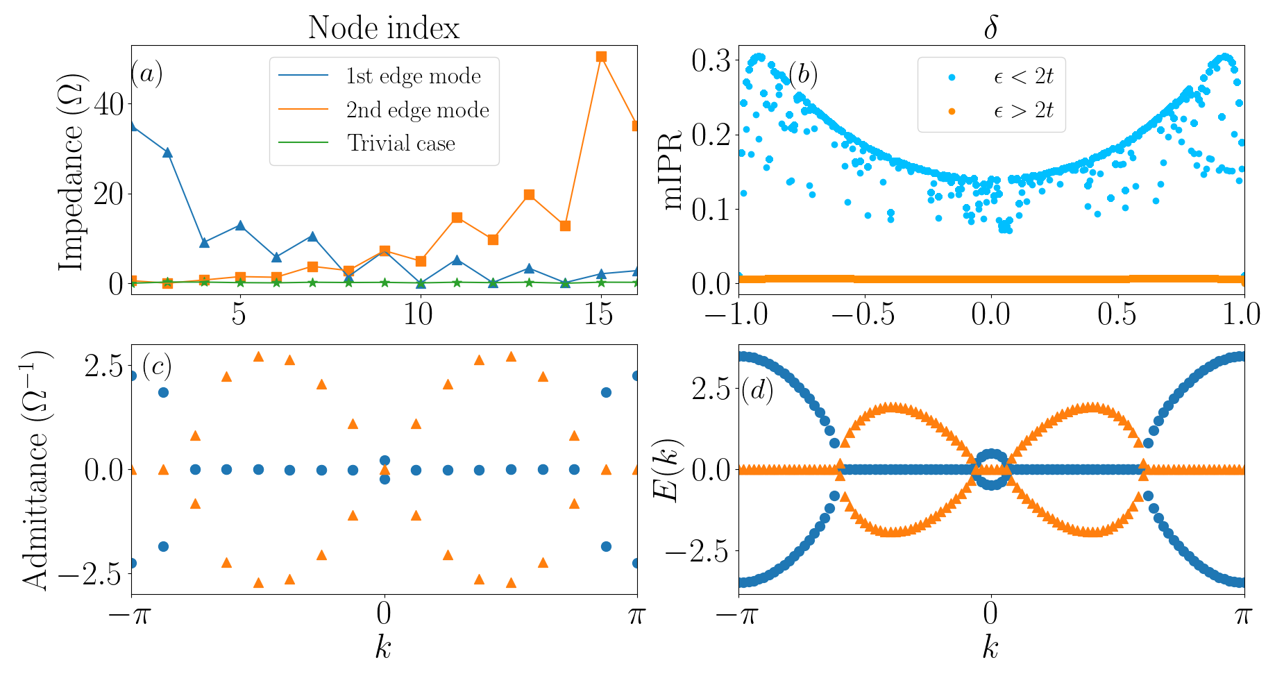
Figure 6: (a) The IP for $\mathcal{PT}$-symmetric NH circuit. The plot is obtained with the same values of circuit elements used for the Hermitian case with OBC and fixing the value of $|C^{\prime}|$ at $15\;\mu F$, which is always less than $C_{2}$. (b) The mIPR for $\mathcal{PT}$-symmetric NH lattice model is varied with $\delta$ for $t=t_{ps}=1$ corresponding to the cases $\epsilon=1.5$ ($<2t$) and $\epsilon=3$ ($>2t$), respectively. (c) The ABS of the circuit is shown. All the values of the circuit elements remain the same as the Hermitian circuit, except for $C_{1}$, $L_{1}$ and $C^{\prime},$ which are $15\;\mu F$, $39\;\mu H$ and $34\;\mu F$. (d) The band structure of the lattice model for $\epsilon=\delta=1.5$. The real and imaginary parts of the admittance (and the lattice band structures) are represented by circles and triangles, respectively.

Now, we shall analyse the circuit with PBC through the Bloch Hamiltonian, $J_{NH_{2}}$, given by,

$$J_{NH_{2}}(\omega,k)=\left[\left(\frac{1}{i\omega L_{1}}+i\omega(C_{2}+C_{3})+\frac{2}{i\omega L_{1}}\cos k\right)\sigma_{z}+\frac{2}{i\omega L_{2}}\sin k\;\sigma_{y}+2i\omega C_{x}\sin k\;\sigma_{x}\right].$$ (15)

Using this equation, we get the plot for ABS, shown in Fig.6(c). The results clearly show that the admittance values are either purely real or purely imaginary, suggesting the circuit is in $\mathcal{PT}$-broken phase, as the $\mathcal{PT}$-unbroken phase possesses only real eigenvalues. If we consider the Bloch Hamiltonian of an abstract circuit, denoted as $J_{NH_{2}}^{\prime}(\omega,k)$ corresponding to $h_{3}^{\prime}(k)$ in Eq.(13), it will yield results similar to those shown in Fig.6(c). This similarity arises because $J_{NH_{2}}(\omega,k)$ and $J_{NH_{2}}^{\prime}(\omega,k)$ are linked through the unitary transformation specified in Eq.(12). On a parallel front, for the non-reciprocal TB model, the expression for energy, which is the same for both $h_{3}(k)$ and $h^{\prime}_{3}(k)$, is given by,

$$E_{3\pm}(k)=\pm\sqrt{(-\epsilon+2t\cos k)^{2}+4(t_{ps}^{2}-\delta^{2})\sin^{2}k}.$$ (16)

The corresponding band structure to the above equation is shown in Fig.6(c). Upon closer examination of Eq.(16), we can discern that the condition for the system to exist in the $\mathcal{PT}$-unbroken phase is expressed as $\epsilon>2\sqrt{\delta^{2}+t^{2}-t_{ps}^{2}}$. This inequality translates to the condition $C_{2}+C_{3}>C_{1}+2\sqrt{C_{x}^{2}+C_{1}^{2}-C_{2}^{2}}$ for the circuit. The parameters used for both the plots in Figs. 6(c) and 6(d) do not satisfy the above conditions, owing to the energy being complex and indicating that they belong to the $\mathcal{PT}$-broken phase. Last but not least, the real and the imaginary parts of the energy eigenvalues constitute a line gap, which again hints toward the absence of NHSE.

III Conclusion

In this comprehensive study, we have explored topoelectrical circuits inspired by a two-orbital, one-dimensional TB model, encompassing both Hermitian and non-Hermitian variants. The key distinctions between these models lie in their symmetries and the critical values of the parameters, namely, the inter-orbital ($t_{ps}$) and intra-orbital ($t$) hopping amplitudes governing the transition from trivial to topological phases. While the $\mathcal{PT}$ symmetry is absent in the model with an imaginary onsite potential, it remains intact in the non-reciprocal model. The localisation characteristics are suitably captured by examining the maximum inverse participation ratio. Intriguingly, none of these models exhibits any indications of NHSE, despite a natural expectation that non-reciprocal models typically manifest NHSE. Consequently, both the models preserve the BBC and feature a line gap as their complex energy gap. For the $\mathcal{PT}$-symmetric case, the system hosts purely real eigenvalues in the $\mathcal{PT}$-unbroken regime, while complex eigenvalues emerge in the $\mathcal{PT}$-broken phase. We have constructed topoelectrical circuits for all the three models to bridge the gap between theory and experiment. The IP of each circuit faithfully mimics the edge modes of the corresponding TB models pertaining to the topological phase. Additionally, the ABS of the circuit networks with PBC accurately yields the energy band structure of the corresponding models. In essence, this work offers a holistic perspective on the experimental verification of topological phenomena in NH systems through electronic circuits, shedding light on both the theoretical underpinnings and practical considerations of this intriguing field of study.

References

- [1] Su, W. P., Schrieffer, J. R. & Heeger, A. J. Solitons in Polyacetylene Phys. Rev. Lett. 42, 1698-1701 (1979)
- [2] Klitzing, K. v., Dorda, G. & Pepper, M. New Method for High-Accuracy Determination of the Fine-Structure Constant Based on Quantized Hall Resistance Phys. Rev. Lett. 45, 494-497 (1980)
- [3] Hasan, M. Z. & Kane, C. L. Colloquium: Topological insulators Rev. Mod. Phys. 82, 3045-3067 (2010)
- [4] Qi, Xiao-Liang & Zhang, Shou-Cheng Topological insulators and superconductors Rev. Mod. Phys. 83, 1057-1110 (2011)
- [5] Bansil, A., Lin, Hsin & Das, Tanmoy Colloquium: Topological band theory Rev. Mod. Phys. 88, 021004 (2016)
- [6] Chiu, Ching-Kai, Teo, Jeffrey C. Y., Schnyder, Andreas P. & Ryu, Shinsei Classification of topological quantum matter with symmetries Rev. Mod. Phys. 88, 035005 (2016)
- [7] Shinsei Ryu, Andreas P Schnyder, Akira Furusaki and Andreas W W Ludwig Topological insulators and superconductors: tenfold way and dimensional hierarchy New J. Phys. 12, 065010 (2010)
- [8] Bender, Carl M. & Boettcher, Stefan Real Spectra in Non-Hermitian Hamiltonians Having PT Symmetry Phys. Rev. Lett. 80, 5243-5246 (1998)
- [9] Lee, Tony E. Anomalous Edge State in a Non-Hermitian Lattice Phys. Rev. Lett. 116, 133903 (2016)
- [10] Shen, Huitao, Zhen, Bo & Fu, Liang Topological Band Theory for Non-Hermitian Hamiltonians Phys. Rev. Lett. 120, 146402 (2018)
- [11] Kohei Kawabata, Ken Shiozaki, Masahito Ueda, and Masatoshi Sato Symmetry and Topology in Non-Hermitian Physics Phys. Rev. X 9, 041015 (2019)
- [12] Kunst, Flore K., Edvardsson, Elisabet, Budich, Jan Carl & Bergholtz, Emil J. Biorthogonal Bulk-Boundary Correspondence in Non-Hermitian Systems Phys. Rev. Lett. 121, 026808 (2018)
- [13] Martinez Alvarez, V. M., Barrios Vargas, J. E. & Foa Torres, L. E. F. Non-Hermitian robust edge states in one dimension: Anomalous localisation and eigenspace condensation at exceptional points Phys. Rev. B 97, 121401 (2018)
- [14] Ching Hua Lee & Ronny Thomale Anatomy of skin modes and topology in non-Hermitian systems Phys. Rev. B 99, 201103 (2019)
- [15] C. Yuce Non-Hermitian anomalous skin effect Physics Letters A 384, 126094 (2020)
- [16] Okuma, Nobuyuki, Kawabata, Kohei, Shiozaki, Ken & Sato, Masatoshi Topological Origin of Non-Hermitian Skin Effects Phys. Rev. Lett. 124, 086801 (2020)
- [17] Kawabata, Kohei, Sato, Masatoshi & Shiozaki, Ken Higher-order non-Hermitian skin effect Phys. Rev. B 102, 205118 (2020)
- [18] Yao, Shunyu & Wang, Zhong Edge States and Topological Invariants of Non-Hermitian Systems Phys. Rev. Lett. 121, 086803 (2018)
- [19] Yokomizo, Kazuki & Murakami, Shuichi Non-Bloch Band Theory of Non-Hermitian Systems Phys. Rev. Lett. 123, 066404 (2019)
- [20] Simon Lieu Topological phases in the non-Hermitian Su-Schrieffer-Heeger model Phys. Rev. B 97, 045106 (2018)
- [21] W D Heiss The physics of exceptional points J. Phys. A: Math. Theor. 45 444016 (2012)
- [22] Leykam, Daniel, Bliokh, Konstantin Y., Huang, Chunli, Chong, Y. D. & Nori, Franco Edge Modes, Degeneracies, and Topological Numbers in Non-Hermitian Systems Phys. Rev. Lett. 118, 040401 (2017)
- [23] Rüter, C., Makris, K., El-Ganainy, R. et al. Observation oparity–time symmetry in optics Nature Phys 6, 192–195 (2010)
- [24] T. Eichelkraut et al., Mobility transition from ballistic to diffusive transport in non-Hermitian lattices Nat. Commun. 4 (2013)
- [25] Albert, Victor V., Glazman, Leonid I. & Jiang, Liang Topological Properties of Linear Circuit Lattices Phys. Rev. Lett. 114, 173902 (2015)
- [26] Ningyuan, Jia, Owens, Clai, Sommer, Ariel, Schuster, David & Simon, Jonathan Time- and Site-Resolved Dynamics in a Topological Circuit Phys. Rev. X 5, 021031 (2015)
- [27] Lee, C.H., Imhof, S., Berger, C. et al. Topolectrical Circuits Commun Phys 1, 39 (2018)
- [28] Wang et al., Non-Hermitian topology in static mechanical metamaterials Sci. Adv. 9, eadf7299 (2023)
- [29] Fleury, Romain, Sounas, Dimitrios & Alù, Andrea An invisible acoustic sensor based on parity-time symmetry Nat. Commun. 16 (2015)
- [30] Gu, Zhongming, Gao, He, Cao, Pei-Chao, Liu, Tuo, Zhu, Xue-Feng & Zhu, Jie Controlling Sound in Non-Hermitian Acoustic Systems Phys. Rev. Appl. 16, 057001 (2021)
- [31] Helbig, Tobias, Hofmann, Tobias, Lee, Ching Hua, Thomale, Ronny, Imhof, Stefan, Molenkamp, Laurens W. & Kiessling, Tobias Band structure engineering and reconstruction in electric circuit networks Phys. Rev. B 99, 161114 (2019)
- [32] Motohiko Ezawa Braiding of Majorana-like corner states in electric circuits and its non-Hermitian generalisation Phys. Rev. B 100, 045407 (2019)
- [33] Li, L., Lee, C.H., Mu, S. et al. Critical non-Hermitian skin effect Nat Commun 11, 5491 (2020)
- [34] Tobias Hofmann, Tobias Helbig et al. Reciprocal skin effect and its realisation in a topolectrical circuit Phys. Rev. Research 2, 023265 (2020)
- [35] Helbig, T., Hofmann, T., Imhof, S. et al. Generalised bulk–boundary correspondence in non-Hermitian topolectrical circuits Nat. Phys. 16, 747–750 (2020)
- [36] Lang, Li-Jun, Weng, Yijiao, Zhang, Yunhui, Cheng, Enhong & Liang, Qixia Dynamical robustness of topological end states in non-reciprocal Su-Schrieffer-Heeger models with open boundary conditions Phys. Rev. B 103, 014302 (2021)
- [37] Junkai Dong, Vladimir Juričić, and Bitan Roy Topolectric circuits: Theory and construction Phys. Rev. Research 3, 023056 (2021)
- [38] S. M. Rafi-Ul-Islam, Zhuo Bin Siu, Haydar Sahin, Ching Hua Lee, and Mansoor B. A. Jalil Unconventional skin modes in generalised topolectrical circuits with multiple asymmetric couplings Phys. Rev. Research 4, 043108 (2022)
- [39] Zhang, Hanxu, Chen, Tian, Li, Linhu, Lee, Ching Hua & Zhang, Xiangdong Electrical circuit realisation of topological switching for the non-Hermitian skin effect Phys. Rev. B 107, 085426 (2023)
- [40] Ganguly, S., Maiti, S.K. Electrical analogue of one-dimensional and quasi-one-dimensional Aubry–André–Harper lattices Sci Rep 13, 13633 (2023)
- [41] F Y Wu Theory of resistor networks: the two-point resistance J. Phys. A: Math. Gen. 37, 6653 (2004)
- [42] Alexander Stegmaier et al. Topological Defect Engineering and PT Symmetry in Non-Hermitian Electrical Circuits Phys. Rev. Lett. 126, 215302 (2021)
- [43] B Kramer and A MacKinnon Localization: theory and experiment Rep. Prog. Phys. 56, 1469 (1993)