Spectrum Sharing between UAV-based Wireless Mesh Networks and Ground Networks

Abstract

The unmanned aerial vehicle (UAV)-based wireless mesh networks can economically provide wireless services for the areas with disasters. However, the capacity of air-to-air communications is limited due to the multi-hop transmissions. In this paper, the spectrum sharing between UAV-based wireless mesh networks and ground networks is studied to improve the capacity of the UAV networks. Considering the distribution of UAVs as a three-dimensional (3D) homogeneous Poisson point process (PPP) within a vertical range, the stochastic geometry is applied to analyze the impact of the height of UAVs, the transmit power of UAVs, the density of UAVs and the vertical range, etc., on the coverage probability of ground network user and UAV network user, respectively. The optimal height of UAVs is numerically achieved in maximizing the capacity of UAV networks with the constraint of the coverage probability of ground network user. This paper provides a basic guideline for the deployment of UAV-based wireless mesh networks.

I Introduction

Since unmanned aerial vehicles (UAVs) have flexible maneuverability and large coverage, the UAV-mounted base stations (BSs) are widely applied to provide ubiquitous wireless connections [1]. The UAV-mounted BSs relieve the mismatch between the diverse traffic load and the fixed infrastructures [2]. For example, the demand for mobile and flexible wireless connections is urgent in the areas with traffic congestions or concerts. UAV-mounted BSs can be deployed in this scenario to offload the cellular traffic to the UAVs [3]. In the areas with disasters, the ground infrastructures are destroyed and the UAV-mounted BSs can be deployed to provide communication services to the rescue persons and vehicles on ground [4, 5].

In the UAV-mounted BS system, multiple small UAVs can provide more economical wireless coverage than a single large UAV [6]. Li et al. in [7] developed a two-UAV relaying system to extend the communication range of UAV networks. They have verified the feasibility of realizing multi-UAV communications. Chand et al. in [8] designed a UAV-based wireless mesh network for the scenarios of disaster management and military environment. The project loon established by Alphabet Inc. aims to provide Internet access to remote areas using balloons which form an aerial mesh network [9]. In [10], we have realized the UAV-based wireless mesh network, where multiple UAVs provide wireless coverage to the users on ground. Meanwhile, the UAVs form an aerial ad hoc network. With one UAV accessing the Internet via the gateway, all the users on ground can access the Internet.

According to Gupta and Kumar’s theory [11], the per-node capacity of ad hoc networks is a decreasing function of the number of hops. For the aerial tier in the UAV-based mesh network, the multi-hop transmissions bring severe capacity shortage problem for each UAV. Spectrum sharing is an effective technology in improving the capacity of wireless networks via enhancing the spectrum utilization. Fortunately, the UAV networks and ground networks such as cellular networks are spatially separated, which creates a unique opportunity for the spectrum sharing between them [12]. Zhang et al. in [14] studied the spectrum sharing between the drone small cell networks and the cellular networks. Sboui et al. in [15] optimized the transmit power to maximize the energy efficiency when a UAV shares the spectrum of primary users. Lyu et al. in [16] designed the orthogonal spectrum sharing between UAV and ground BS. Yoshikawa et al. in [17] studied the spectrum sharing between UAVs and radar systems. Huang et al. in [18] designed the routing schemes for the aerial cognitive radio networks.

Although many prior works have studied the issue of spectrum sharing between UAVs and other wireless systems, to the best of the authors’ knowledge, very few studies have considered the issue of spectrum sharing between the UAV-based wireless mesh networks and the ground networks, such as cellular networks. Motivated by this, in this paper, the spectrum sharing is studied in the air-to-air communications of UAVs to improve the capacity of UAV networks. Considering the distribution of UAVs as a three-dimensional (3D) homogeneous Poisson point process (PPP), stochastic geometry is applied to analyze the coverage probability of UAV network users and ground network users. As a result, the optimal height of UAVs can be found with the constraint of the coverage probability of ground network users.

The remainder of this paper is organized as follows. In Section II, the system model is introduced. Section III analyzes the performance of spectrum sharing of UAV-ground networks using stochastic geometry. The simulation results are provided in Section IV. Finally, we summarize this paper in Section V.

II System Model

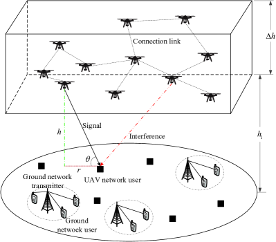
Figure 1: System model of UAV-ground spectrum sharing.

When multiple UAVs provide wireless services to the users on ground, the UAVs should form a wireless mesh network to improve the coverage of the multiple UAVs. In this scenario, each UAV acts as an aerial BS and the multiple UAVs form an aerial ad hoc network. With one UAV connecting to the gateway via backhaul link, all the UAVs can provide Internet connections for the UAV network users. In the aerial ad hoc networks, multi-hop transmissions are required to forward data from sources to destinations. Since multi-hop transmissions bring severe capacity shortage problem for each UAV, the communications among UAVs share the spectrum of the ground networks to improve the network capacity. While the spectrum of the air-to-ground communications is different from the spectrum of the ground networks to avoid the severe interference between them.

II-A Network model

As illustrated in Fig. 1, the distribution of the transmitters (TXs) of ground network, such as the BSs of cellular network, follows a two-dimensional (2D) homogeneous PPP ${\Phi_{d}}$ with density ${\lambda_{d}}$. The distribution of UAVs follows a 3D homogeneous PPP ${\Phi_{u}}$ with density ${\lambda_{u}}$. The minimum and maximum heights of UAVs are $h_{1}$ and $h_{1}+\Delta h$, respectively. $\Delta h$ is defined as the vertical range of the UAVs. In the UAV network, the Aloha protocol is applied as the medium access control (MAC) protocol.

II-B Channel model

Both path-loss and small scale fading are considered. The path-loss exponent of the ground-to-ground link is $\alpha_{d}$. The path-loss exponent of the air-to-ground link is $\alpha_{u}$. The power gain of small scale fading is an exponential distributed random variable with unit mean. Additive white Gaussian noise is considered with mean zero and variance $N$. The transmit power of the UAV and the TX of ground network are $P_{u}$ and $P_{d}$, respectively. Both the line-of-sight (LoS) and non-line-of-sight (NLoS) propagations in the air-to-ground communications are considered. The received signal strength at the UAV network user can be expressed as [19, 20]

$${P_{r,g}}=\left\{{\begin{array}[]{*{20}{c}}{{P_{u}}{{\left|{{d_{ug}}}\right|}^{-{\alpha_{u}}}}}&{{\rm{LoS}}}\\ {\eta{P_{u}}{{\left|{{d_{ug}}}\right|}^{-{\alpha_{u}}}}}&{{\rm{NLoS}}}\end{array}}\right.,$$ (1)

where ${{d_{ug}}}$ is the distance between the UAV and the UAV network user. $\eta$ is an attenuation factor because of the NLoS propagation [19]. The probability of LoS propagation is as follows [20].

$${P_{\rm{LoS}}}=\frac{1}{{1+C\exp\left({-B(\theta-C)}\right)}},$$ (2)

where $B$ and $C$ are environmental dependent constants. $\theta$ is the elevation angle. As illustrated in Fig. 1, with $h$ being the height of a UAV and $r$ being the distance between the projection of the UAV on ground and the UAV network user, the value of $\theta$ is

$$\theta=\frac{{180}}{\pi}\arctan({\frac{h}{r}}).$$ (3)

III Spectrum Sharing of UAV-Ground Networks

$${L_{I_{gu}^{c}}}({\frac{{\beta{d_{0}}^{{\alpha_{d}}}}}{{{P_{d}}}}})=\exp({-\frac{{2\lambda_{d}{\pi^{2}}{{\left(\beta\right)}^{2/{\alpha_{d}}}}{d_{0}}^{2}}}{{{\alpha_{d}}\sin\left({2\pi/{\alpha_{d}}}\right)}}})$$ (4)

$${L_{{I_{u,LOS}}}}({\frac{{\beta d_{0}^{{\alpha_{d}}}}}{{{P_{d}}}}}) =\exp({-{\lambda_{u}}\int\limits_{V}{({1-\frac{1}{{1+\frac{{\beta d_{0}^{{\alpha_{d}}}}}{{{P_{d}}}}{P_{u}}{P_{LOS}}x_{i}^{-{\alpha_{u}}}}}})}dx})$$ (5)

$$=\exp({-{\lambda_{u}}\int_{h1}^{h2}{\int_{0}^{2\pi}{\int_{0}^{\infty}{({1-\frac{1}{{1+\frac{{\beta d_{0}^{{\alpha_{d}}}}}{{{P_{d}}}}{P_{u}}{{(\sqrt{{r^{2}}+{z^{2}}})}^{-{\alpha_{u}}}}\frac{1}{{1+C\exp({-B(\frac{{180}}{\pi}\arctan(z/r)-C)})}}}}})}}}rdrd\phi dz})$$

$$=\exp({-2\pi{\lambda_{u}}{H_{1}}({\beta,{d_{0}},h,{\alpha_{d}},{\alpha_{u}}})}).$$

$${L_{{I_{u,{\text{NLoS}}}}}}({\frac{{\beta d_{0}^{{\alpha_{d}}}}}{{{P_{d}}}}}) =\exp({-2\pi{\lambda_{u}}\int_{h1}^{h2}{\int_{0}^{\infty}{({1-\frac{1}{{1+\frac{{\beta d_{0}^{{\alpha_{d}}}}}{{{P_{d}}}}{P_{u}}\eta{{(\sqrt{{r^{2}}+{z^{2}}})}^{-{\alpha_{u}}}}(1-\frac{1}{{1+C\exp({-B(\frac{{180}}{\pi}\arctan(z/r)-C)})}})}}})}}rdrdz})$$ (6)

$$=\exp({-2\pi{\lambda_{u}}{H_{2}}({\beta,{d_{0}},h,{\alpha_{d}},{\alpha_{u}}})}).$$

$${H_{1}}({\beta,{d_{0}},h,{\alpha_{d}},{\alpha_{u}}})=\int_{h1}^{h2}{\int_{0}^{\infty}{({1-\frac{1}{{1+\frac{{\beta d_{0}^{{\alpha_{d}}}}}{{{P_{d}}}}{P_{u}}{{(\sqrt{{r^{2}}+{z^{2}}})}^{-{\alpha_{u}}}}\frac{1}{{1+C\exp({-B(\frac{{180}}{\pi}\arctan(z/r)-C)})}}}}})}}rdrdz.$$ (7)

$${H_{2}}({\beta,{d_{0}},h,{\alpha_{d}},{\alpha_{u}}})=\int_{h1}^{h2}{\int_{0}^{\infty}{({1-\frac{1}{{1+\frac{{\beta d_{0}^{{\alpha_{d}}}}}{{{P_{d}}}}{P_{u}}\eta{{(\sqrt{{r^{2}}+{z^{2}}})}^{-{\alpha_{u}}}}(1-\frac{1}{{1+C\exp({-B(\frac{{180}}{\pi}\arctan(z/r)-C)})}})}}})}}rdrdz.$$ (8)

With the spectrum sharing between the UAV network and the ground network, we derive the coverage probabilities of ground network user and UAV network user respectively.

The coverage probability is defined as the probability of successful communication. Define $\beta$ as the threshold of signal-to-interference-plus-noise ratio (SINR) at the receiver for successfully communication. The coverage probability is the probability $P(\gamma>\beta)$ with $\gamma$ being the SINR of the receiver.

III-A The coverage probability of ground network user

Define ${\gamma_{gu}}=\frac{{{P_{d}}d_{0}^{-{\alpha_{d}}}{g_{0}}}}{{I_{gu}^{c}+{I_{u}}+N}}$ as the received SINR of a typical ground network user at the origin $\{\bf{0}\}$, where $g_{0}$ is the power gain of small scale fading. $d_{0}$ is the distance between the typical ground network user and its associated TX. ${I_{gu}^{c}}$ and ${{I_{u}}}$ are the interference generated by the TXs of ground network and the UAVs, respectively.

$$I_{gu}^{c}=\sum\limits_{{d_{i}}\in{\Phi_{d}}\backslash\{\bf{0}\}}{{P_{d}}}d_{i}^{-{\alpha_{d}}}{g_{i}},$$ (9)

$${I_{u}} ={I_{u,LoS}}+{I_{u,{\rm{NLoS}}}}$$ (10)

$$=\sum\limits_{{x_{i}}\in{\Phi_{u}}}{{P_{{\rm{LoS}}}}{P_{u}}}x_{i}^{-{\alpha_{d}}}{g_{i}}+\sum\limits_{{x_{i}}\in{\Phi_{u}}}{\left({1-{P_{{\rm{LoS}}}}}\right)\eta{P_{u}}}x_{i}^{-{\alpha_{d}}}{g_{i}},$$

where $g_{i}$ is the small scale fading gain of the interference link. $d_{i}$ is the distance between the $i$th TX of ground network and the typical ground network user. $x_{i}$ is the distance between the $i$th UAV and the typical ground network user.

With the definition of the coverage probability, the coverage probability of a typical ground network user is

$${P_{1}} =P({\gamma_{gu}}>\beta),$$ (11)

$$\mathop{=}\limits^{(a)}\exp({-\frac{{\beta d_{0}^{{\alpha_{d}}}({I_{gu}^{c}+{I_{u}}+N})}}{{{P_{d}}}}})$$

$$=\exp({-\frac{{\beta d_{0}^{{\alpha_{d}}}I_{gu}^{c}}}{{{P_{d}}}}})\exp({-\frac{{\beta d_{0}^{{\alpha_{d}}}{I_{u}}}}{{{P_{d}}}}})\exp({-\frac{{\beta d_{0}^{{\alpha_{d}}}N}}{{{P_{d}}}}})$$

$$={L_{I_{gu}^{c}}}({\frac{{\beta d_{0}^{{\alpha_{d}}}}}{{{P_{d}}}}}){L_{{I_{u}}}}({\frac{{\beta d_{0}^{{\alpha_{d}}}}}{{{P_{d}}}}})\exp({-\frac{{\beta d_{0}^{{\alpha_{d}}}N}}{{{P_{d}}}}}),$$

where $(a)$ is obtained from the exponential distribution of $g_{0}$. ${L_{A}}(*)$ is the Laplace transform of the random variable $A$.

With the considered path-loss model (1), $I_{u}$ can be re-expressed as

$$I_{u}={I_{u,{\rm{LoS}}}}+{I_{u,{\rm{NLoS}}}}.$$ (12)

The Laplace function of $I_{u}$ then can be expressed as

$${L_{{I_{u}}}}({\frac{{\beta d_{0}^{{\alpha_{d}}}}}{{{P_{d}}}}})={L_{{I_{u,{\rm{LoS}}}}}}({\frac{{\beta d_{0}^{{\alpha_{d}}}}}{{{P_{d}}}}}){L_{{I_{u,N{\rm{LoS}}}}}}({\frac{{\beta d_{0}^{{\alpha_{d}}}}}{{{P_{d}}}}}).$$ (13)

Since $g_{i}$ is a random variable independent of the point process ${\Phi_{u}}$, we have

$${L_{{I_{u,{\rm{LoS}}}}}}({\frac{{\beta d_{0}^{{\alpha_{d}}}}}{{{P_{d}}}}})={E_{{I_{u,{\rm{LoS}}}}}}[{\exp({\frac{{\beta d_{0}^{{\alpha_{d}}}}}{{{P_{d}}}}{I_{u,{\rm{LoS}}}}})}]$$ (14)

$$={E_{{g_{i}},{\Phi_{u}}}}[{\prod\limits_{{x_{i}}\in{\Phi_{u}}\backslash\{\bf{0}\}}{\exp({\frac{{\beta d_{0}^{{\alpha_{d}}}}}{{{P_{d}}}}{g_{i}}{P_{u}}{P_{{\rm{LoS}}}}x_{i}^{-{\alpha_{u}}}})}}]$$

$$={E_{{\Phi_{u}}}}[{\prod\limits_{{x_{i}}\in{\Phi_{u}}\backslash\{\bf{0}\}}{{E_{{g_{i}}}}[\exp({\frac{{\beta d_{0}^{{\alpha_{d}}}}}{{{P_{d}}}}{P_{u}}{P_{{\rm{LoS}}}}x_{i}^{-{\alpha_{u}}}})]}}]$$

$$={E_{{\Phi_{u}}}}[{\prod\limits_{{x_{i}}\in{\Phi_{u}}\backslash\{\bf{0}\}}{\frac{1}{{1+\frac{{\beta d_{0}^{{\alpha_{d}}}}}{{{P_{d}}}}{P_{u}}{P_{{\rm{LoS}}}}x_{i}^{-{\alpha_{u}}}}}}}],$$

and

$${L_{{I_{u,{\rm{NLoS}}}}}}({\frac{{\beta d_{0}^{{\alpha_{d}}}}}{{{P_{d}}}}})$$ (15)

$$={E_{{\Phi_{u}}}}[{\prod\limits_{{x_{i}}\in{\Phi_{u}}\backslash\{\bf{0}\}}{\frac{1}{{1+\frac{{\beta d_{0}^{{\alpha_{d}}}}}{{{P_{d}}}}{P_{u}}(1-{P_{{\rm{LoS}}}})\eta x_{i}^{-{\alpha_{u}}}}}}}].$$

Hence, ${L_{{I_{u}}}}({\frac{{\beta d_{0}^{{\alpha_{d}}}}}{{{P_{d}}}}})$ is derived as follows.

$${L_{{I_{u}}}}({\frac{{\beta d_{0}^{{\alpha_{d}}}}}{{{P_{d}}}}})={E_{{\Phi_{u}}}}[{\prod\limits_{{x_{i}}\in{\Phi_{u}}}{\frac{1}{{1+\frac{{\beta d_{0}^{{\alpha_{d}}}}}{{{P_{d}}}}{P_{u}}{P_{{\rm{LoS}}}}x_{i}^{-{\alpha_{u}}}}}}}]$$ (16)

$$\times{E_{{\Phi_{u}}}}[{\prod\limits_{{x_{i}}\in{\Phi_{u}}}{\frac{1}{{1+\frac{{\beta d_{0}^{{\alpha_{d}}}}}{{{P_{d}}}}{P_{u}}(1-{P_{{\rm{LoS}}}})\eta x_{i}^{-{\alpha_{u}}}}}}}].$$

Applying the probability generating function of PPP [14]

$$E({\prod\limits_{{x_{i}}\in\Phi}{f(x)}})=\exp({-{\lambda_{d}}\int\limits_{V}{[{1-f(x)}]}dx}),$$ (17)

then ${L_{I_{gu}^{c}}}({\frac{{\beta d_{0}^{{\alpha_{d}}}}}{{{P_{d}}}}})$ can be derived as (4) [13]. ${L_{{I_{u}}}}({\frac{{\beta d_{0}^{{\alpha_{d}}}}}{{{P_{d}}}}})$ can be derived using (5) and (6), where ${H_{1}}({\beta,{d_{0}},h,{\alpha_{d}},{\alpha_{u}}})$ and ${H_{2}}({\beta,{d_{0}},h,{\alpha_{d}},{\alpha_{u}}})$ are provided in (7) and (8), respectively.

$${L_{I_{u,{\rm{LoS}}}^{c}}}({\frac{{\beta x_{0}^{{\alpha_{u}}}}}{{{P_{u}}}}}) =\exp({-{\lambda_{u}}\int\limits_{V}{({1-\frac{1}{{1+\beta x_{0}^{{\alpha_{u}}}{P_{{\rm{LoS}}}}x_{i}^{-{\alpha_{u}}}}}})}dx})$$ (18)

$$=\exp({-{\lambda_{u}}\int_{h1}^{h2}{\int_{0}^{2\pi}{\int_{0}^{\infty}{({1-\frac{1}{{1+\beta x_{0}^{{\alpha_{u}}}{{(\sqrt{{r^{2}}+{z^{2}}})}^{-{\alpha_{u}}}}\frac{1}{{1+C\exp({-B(\frac{{180}}{\pi}\arctan(z/r)-C)})}}}}})}}}rdrd\phi dz})$$

$$=\exp({-2\pi{\lambda_{u}}{H_{3}}({\beta,{x_{0}},h,{\alpha_{u}}})}).$$

$${L_{I_{u,{\rm{NLoS}}}^{c}}}({\frac{{\beta x_{0}^{{\alpha_{u}}}}}{{{P_{u}}}}}) =\exp({-2\pi{\lambda_{u}}\int_{h1}^{h2}{\int_{0}^{\infty}{({1-\frac{1}{{1+\beta x_{0}^{{\alpha_{u}}}\eta{{(\sqrt{{r^{2}}+{z^{2}}})}^{-{\alpha_{u}}}}(1-\frac{1}{{1+C\exp({-B(\frac{{180}}{\pi}arctan(z/r)-C)})}})}}})}}rdrdz})$$ (19)

$$=\exp({-2\pi{\lambda_{u}}{H_{4}}({\beta,{x_{0}},h,{\alpha_{u}}})}).$$

$${H_{3}}({\beta,{x_{0}},h,{\alpha_{u}}})=\int_{h1}^{h2}{\int_{0}^{\infty}{({1-\frac{1}{{1+\beta x_{0}^{{\alpha_{u}}}{{(\sqrt{{r^{2}}+{z^{2}}})}^{-{\alpha_{u}}}}\frac{1}{{1+C\exp({-B(\frac{{180}}{\pi}\arctan(z/r)-C)})}}}}})}}rdrdz.$$ (20)

$${H_{4}}({\beta,{x_{0}},h,{\alpha_{u}}})=\int_{h1}^{h2}{\int_{0}^{\infty}{({1-\frac{1}{{1+\beta x_{0}^{{\alpha_{u}}}\eta{{(\sqrt{{r^{2}}+{z^{2}}})}^{-{\alpha_{u}}}}(1-\frac{1}{{1+C\exp({-B(\frac{{180}}{\pi}\arctan(z/r)-C)})}})}}})}}rdrdz.$$ (21)

III-B The coverage probability of UAV network user

The coverage probability of a typical UAV network user is defined as

$${P_{2}}=P({\gamma_{uu}>\beta}),$$ (22)

where $\gamma_{uu}$ is the received SINR of the UAV network user and $\beta$ is the SINR threshold. With the considered path-loss model (1), ${P_{2}}$ can be expressed as

$$P_{2} ={P_{{\text{LoS}}}}P({\frac{{{P_{u}}x_{0}^{-{\alpha_{u}}}{g_{i}}}}{{I_{u}^{c}}}>\beta})+{P_{{\text{NLoS}}}}P({\frac{{\eta{P_{u}}x_{0}^{-{\alpha_{u}}}{g_{i}}}}{{I_{u}^{c}}}>\beta})$$ (23)

$$={P_{{\text{LoS}}}}\exp({-\frac{{\beta x_{0}^{{\alpha_{u}}}I_{u}^{c}}}{{{P_{u}}}}})+(1-{P_{{\text{LoS}}}})\exp({-\frac{{\beta x_{0}^{{\alpha_{u}}}I_{u}^{c}}}{{\eta{P_{u}}}}})$$

$$={P_{{\text{LoS}}}}{L_{I_{u}^{c}}}({-\frac{{\beta x_{0}^{{\alpha_{u}}}}}{{{P_{u}}}}})+(1-{P_{{\text{LoS}}}}){L_{I_{u}^{c}}}({-\frac{{\beta x_{0}^{{\alpha_{u}}}}}{{\eta{P_{u}}}}}),$$

where $x_{0}$ is the distance between the typical UAV user and its associated UAV. The term $I_{u}^{c}$ is the received interference from UAVs and we have

$$I_{u}^{c} =I_{{}_{u,{\text{LoS}}}}^{c}+I_{{}_{u,{\text{NLoS}}}}^{c}$$ (24)

$$=\sum\limits_{{x_{i}}\in{\Phi_{u}}\backslash\{\bf{0}\}}{{P_{{\text{LoS}}}}{P_{u}}}x_{i}^{-{\alpha_{u}}}{g_{i}}+$$

$$\sum\limits_{{x_{i}}\in{\Phi_{u}}\backslash\{\bf{0}\}}{({1-{P_{{\text{LoS}}}}})\eta{P_{u}}}x_{i}^{-{\alpha_{u}}}{g_{i}}.$$

Similar to the derivation of the coverage probability of ground network user, we have

$${L_{I_{u}^{c}}}({\frac{{\beta x_{0}^{{\alpha_{u}}}}}{{{P_{u}}}}}) ={L_{I_{u,{\text{LoS}}}^{c}}}({\frac{{\beta x_{0}^{{\alpha_{u}}}}}{{{P_{u}}}}}){L_{I_{u,{\text{NLoS}}}^{c}}}({\frac{{\beta x_{0}^{{\alpha_{u}}}}}{{{P_{u}}}}})$$ (25)

$$={E_{{\Phi_{u}}}}[{\prod\limits_{{x_{i}}\in{\Phi_{u}}\backslash\{\bf{0}\}}{\frac{1}{{1+\beta x_{0}^{{\alpha_{u}}}{P_{{\text{LoS}}}}x_{i}^{-{\alpha_{u}}}}}}}]\times\hfill$$

$${E_{{\Phi_{u}}}}[{\prod\limits_{{x_{i}}\in{\Phi_{u}}\backslash\{\bf{0}\}}{\frac{1}{{1+\beta x_{0}^{{\alpha_{u}}}(1-{P_{{\text{LoS}}}})\eta x_{i}^{-{\alpha_{u}}}}}}}].$$

The ${L_{I_{u,{\text{LoS}}}^{c}}}({\frac{{\beta x_{0}^{{\alpha_{u}}}}}{{{P_{u}}}}})$ and ${L_{I_{u,{\text{NLoS}}}^{c}}}({\frac{{\beta x_{0}^{{\alpha_{u}}}}}{{{P_{u}}}}})$ can be derived in (18) and (19), where ${H_{3}}({\beta,{x_{0}},h,{\alpha_{u}}})$ and ${H_{4}}({\beta,{x_{0}},h,{\alpha_{u}}})$ are provided in (20) and (21), respectively.

IV Numerical Results and Analysis

This section provides the numerical results of the coverage probabilities of UAV network user and ground network user. Besides, the transmission capacity of UAV network is defined and maximized. The parameters in the simulations are summarized in Table 1.

TABLE I: Simulation parameters

Parameter	Value
$P_{u}$	5 W
$P_{d}$	0.1 W
$\alpha_{u}$	3
$\alpha_{d}$	4
$B$ and $C$	0.136 and 11.95
$\beta$	0.1
$\eta$	0.1
$\lambda_{u}$	$10^{-4}$ per square meter
$\lambda_{d}$	$10^{-3}$ per square meter
$d_{0}$	10 m
$N$	$10^{-9}$ W

IV-A The coverage probability of ground network user

The coverage probability of a typical ground network user, namely, $P_{1}$ is illustrated in Fig. 2 as a function of $h_{1}$ and $\Delta h$. The 20-point Monte Carlo simulation results are provided in Fig. 2. Each point undergoes 1000 times Monte Carlo simulations. It is verified that the theoretical results, namely, the surface fits well with the points. Notice that when $h_{1}$ is large, for example, when $h_{1}$ is close to 100 m, $P_{1}$ is large. This is due to the fact that when the UAVs are high above the ground, the interference from UAVs to the typical ground network user is small, which will increase the value of $P_{1}$. When $\Delta h$ is increasing, $P_{1}$ is decreasing because the probability of LoS propagation from UAVs to the ground network user is increasing. This discovery is also observed in Fig. 3, which depicts the relation between $P_{1}$ and $h_{1}$ with different values of $\Delta h$. In Fig. 3, when $h_{1}$ is increasing from 0, $P_{1}$ is firstly decreasing because the probability of LoS propagation between the UAV and the ground network user is increasing. When $h_{1}$ exceeds a threshold, $P_{1}$ is increasing with the increase of $h_{1}$ because the propagation path between the UAV and the ground network user becomes long in this case, which will decrease the interference from UAVs to ground network user.

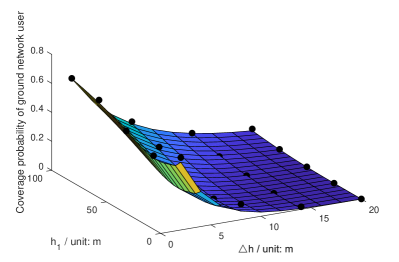
Figure 2: The coverage probability of ground network user versus $h_{1}$ and $\Delta h$.

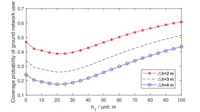
Figure 3: The relation between the coverage probability of ground network user and $h_{1}$ with different values of $\Delta h$.

IV-B The coverage probability of UAV network user

The coverage probability of UAV network user, namely, $P_{2}$ is illustrated in Fig. 4. The 20-point Monte Carlo simulation results are provided in Fig. 4. Each point undergoes 1000 times Monte Carlo simulations. Notice that the theoretical results, namely, the surface fits well with the points. The $P_{2}$ fluctuates with the increase of $h_{1}$. For each $\Delta h$, there exists an optimal $h_{1}$ to maximize $P_{2}$. Besides, with the increase of $\Delta h$, $P_{2}$ is decreasing because the signal link is long. A critical observation is that the when $\Delta h\to 0$, namely, when UAVs are distributed in 2D plane, $P_{2}$ has maximum value in Fig. 4.

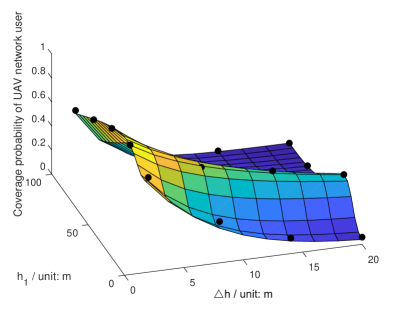
Figure 4: The coverage probability of UAV network user versus $h_{1}$ and $\Delta h$.

IV-C The optimal height of UAVs

The definition of transmission capacity (TC) in [14] is applied to verify the performance of UAV network, which is as follows [14].

$$T_{u}={\lambda_{u}}P(\gamma_{uu}>\beta)\log(1+\beta),$$ (26)

where $\gamma_{uu}$ is the SINR of the UAV network user and $T_{u}$ denotes the TC of UAV network. With the constraint of the coverage probability of ground network user, the optimal height of UAVs, defined as $h_{1}$, can be found to maximize the TC of UAV network. The optimization model is as follows.

$$\mathop{\max}\limits_{{h_{1}}}{\kern 3.0pt}{T_{u}}$$ (27)

$$s.t.{\kern 9.0pt}{P_{1}}\geq\alpha.$$

Although the form of (27) is simple, the object function and constraint condition are complex. It is difficult to derive a closed-form solution. Hence the optimal solution of $h_{1}$ is derived numerically.

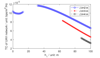
Figure 5: The relation between the transmission capacity of UAV network user and $h_{1}$ with $\alpha=0.4$ and different values of $\Delta h$.

With $\alpha=0.4$, the relation between the TC of UAV network and $h_{1}$ is illustrated in Fig. 5. The optimal $h_{1}$ to maximize the TC of UAV network can be searched. It is verified that with the decrease of $\Delta h$, the TC of UAV network increases. When $\Delta h\to 0$, namely, the UAVs are distributed in a 2D plane, the TC of UAV network is maximum. With the constraint $\alpha=0.4$, there are vacant segments where the $h_{1}$ does not satisfy the constraint of (27). However, when the constraint $\alpha=0.1$, all the values of $h_{1}$ in Fig. 6 are feasible solutions. In this case, the optimal $h_{1}$ can still be searched to maximize the TC of UAV network.

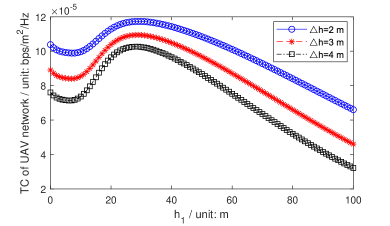
Figure 6: The relation between the transmission capacity of UAV network user and $h_{1}$ with $\alpha=0.1$ and different values of $\Delta h$.

V Conclusion

In this paper, the spectrum sharing between UAV-based wireless mesh networks and ground networks is analyzed using stochastic geometry. The impact of the height of UAVs, the transmit power of UAVs, the density of UAVs and the vertical range on the coverage probability of ground network user and UAV network user is analyzed. Then the optimal height of UAVs is achieved to maximize the transmission capacity of UAV networks. This paper provides fundamental analysis for the spectrum sharing of UAV-based wireless mesh networks, which may motivate the study of spectrum sharing for more aerial wireless mesh networks.

References

- [1] S. Hayat, E. Yanmaz, and R. Muzaffar, “Survey on Unmanned Aerial Vehicle Networks for Civil Applications: A Communications Viewpoint,” IEEE Communications Surveys & Tutorials, vol. 18, no. 4, pp. 2624–2661, Fourth quarter, 2016.
- [2] I. Bor-Yaliniz and H. Yanikomeroglu, “The New Frontier in RAN Heterogeneity: Multi-Tier Drone-Cells,” IEEE Communications Magazine, vol. 54, no. 11, pp. 48–55, Nov. 2016.
- [3] H. Wu, X. Tao, N. Zhang, and X. (Sherman) Shen, “Cooperative UAV Cluster Assisted Terrestrial Cellular Networks with Ubiquitous Coverage,” IEEE Journal on Selected Area in Communications, 2018 (Accepted).
- [4] Y. Zhou, N. Cheng, N. Lu, and X. (Sherman) Shen, “Multi-UAV-Aided Networks: Aerial-Ground Cooperative Vehicular Networking Architecture,” IEEE Vehicular Technology Magazine, vol. 10, no. 4, pp. 36–44, Dec. 2015.
- [5] W. Shi, H. Zhou, J. Li, and et al., “Drone Assisted Vehicular Networks: Architecture, Challenges and Opportunities,” IEEE Network, vol. 32, no. 3, pp. 130–137, May 2018.
- [6] L. Gupta, R. Jain, and G. Vaszkun, “Survey of Important Issues in UAV Communication Networks,” IEEE Communications Surveys & Tutorials, vol. 18, no. 2, pp. 1123–1152, Second quarter, 2016.
- [7] B. Li, Y. Jiang, J. Sun, and et al., “Development and Testing of a Two-UAV Communication Relay System,” Sensors, vol. 16, no. 10, pp. 1–21, Oct. 2016.
- [8] G. S. L. K. Chand, M. Lee, S. Y. Shin, “Drone Based Wireless Mesh Network for Disaster/Military Environment,” Journal of Computer and Communications, vol. 6, pp. 44–52, Apr. 2018.
- [9] S. Levy, “How Google Will Use High-Flying Balloons to Deliver Internet to the Hinterlands,” Wired Retrieved, Jun. 2013.
- [10] Y. Wang, Z. Wei, X. Chen, and et al., “Demo: UAV Assisted Adaptive Aerial Internet,” IEEE/CIC International Conference on Communications in China (ICCC), pp. 1–2, Beijing, Aug. 2018 (Accepted).
- [11] P. Gupta and P. R. Kumar, “The capacity of wireless networks,” IEEE Transactions on Information Theory, vol. 46, no. 2, pp. 388–404, Mar. 2000.
- [12] P. Jacob, R. P. Sirigina, A. S. Madhukumar, and et al., “Cognitive Radio for Aeronautical Communications: A Survey,” IEEE Access, vol. 4, pp. 3417–3443, May 2016.
- [13] Haenggi, Martin and Ganti, Radha Krishna, “Interference in Large Wireless Networks,“ Now Publishers Inc, pp. 127-248, 2009.
- [14] C. Zhang and W. Zhang, “Spectrum Sharing for Drone Networks,” IEEE Journal on Selected Areas in Communications, vol. 35, no. 1, pp. 136–144, Jan. 2017.
- [15] L. Sboui, H. Ghazzai, Z. Rezki, and et al., “Energy-Efficient Power Allocation for UAV Cognitive Radio Systems,” IEEE Vehicular Technology Conference (VTC-Fall), pp. 1–5, Toronto, Sep. 2017.
- [16] J. Lyu, Y. Zeng, and R. Zhang, “Spectrum Sharing and Cyclical Multiple Access in UAV-Aided Cellular Offloading,” IEEE Global Communications Conference (GLOBECOM), pp. 1–6, Singapore, Dec. 2017.
- [17] K. Yoshikawa, S. Yamashita, K. Yamamoto, and et al., “Resource Allocation for 3D Drone Networks Sharing Spectrum Bands,” IEEE Vehicular Technology Conference (VTC-Fall), pp. 1–5, Toronto, Sep. 2017.
- [18] X. Huang, G. Wang, F. Hu, and et al., “Stability-Capacity-Adaptive Routing for High-Mobility Multihop Cognitive Radio Networks,” IEEE Transactions on Vehicular Technology, vol. 60, no. 6, pp. 2714–2729, Jul. 2011.
- [19] M. Mozaffari, W. Saad, M. Bennis, and et al., “Unmanned Aerial Vehicle with Underlaid Device-to-Device Communications: Performance and Tradeoffs,” IEEE Transactions on Wireless Communications, vol. 15, no. 6, pp. 3949–3963, Jun. 2016.
- [20] A. Hourani, K. Sithamparanathan, and S. Lardner, “Optimal LAP altitude for maximum coverage,” IEEE Wireless Communications Letters, vol. 3, no. 6, pp. 569–572, Dec. 2014.