Combining chromomagnetic and four-fermion operators with leading SMEFT operators for $gg\to hh$ at NLO QCD

Abstract

We present the calculation of the contribtuions from the chromomagnetic and four-top-quark-operators within Standard Model Effective Field Theory (SMEFT) to Higgs boson pair production in gluon fusion, combined with full NLO QCD corrections. We study the effects of these operators on the total cross section and the invariant mass distribution of the Higgs-boson pair, at $\sqrt{s}=13.6$ TeV. These subleading operators are implemented in the generator ggHH_SMEFT, in the same Powheg-Box-V2 framework as the leading operators, such that their effects can be easily studied in a unified setup.

1 Introduction

Where is New Physics? If it resides at energy scales well separated from the electroweak scale, our ignorance about its exact nature can be parametrised within an Effective Field Theory (EFT) framework Weinberg:1978kz ; Buchmuller:1985jz ; Isidori:2023pyp .

Predictions for key LHC processes within Standard Model Effective Field Theory (SMEFT) Grzadkowski:2010es ; Brivio:2017vri up to the level of dimension-6 operators, in combination with NLO QCD corrections, have become available in the last few years, see e.g. Refs. Mimasu:2015nqa ; Alioli:2018ljm ; Degrande:2020evl ; Baglio:2020oqu ; Battaglia:2021nys ; Dawson:2021ofa ; Brivio:2021xhp ; Heinrich:2022idm ; Buchalla:2022igv . In addition, the importance of renormalisation group running effects of the Wilson coefficients, calculated up to one loop in Refs. Jenkins:2013zja ; Jenkins:2013wua ; Alonso:2013hga , has gained increasing attention Battaglia:2021nys ; Aoude:2022aro ; Chala:2021wpj ; Dawson:2022ewj and is implemented in dedicated tools Aebischer:2018bkb ; Fuentes-Martin:2020zaz ; DiNoi:2022ejg ; Fuentes-Martin:2022jrf ; Machado:2022ozb ; Martin:2023fad ; Dedes:2023zws ; terHoeve:2023pvs . The effect of double insertions of dimension-6 operators at the level of squared amplitudes also has been studied in the literature Dawson:2021xei ; Ellis:2022zdw ; Alioli:2022fng ; GomezAmbrosio:2022mpm ; Allwicher:2022gkm ; Asteriadis:2022ras .

Here we will focus on Higgs boson pair production in gluon fusion, combining the NLO QCD corrections with full top quark mass dependence with anomalous couplings within SMEFT. The full NLO QCD corrections have been calculated in Refs. Borowka:2016ehy ; Borowka:2016ypz ; Baglio:2018lrj ; Baglio:2020ini , based on numerical evaluations of the two-loop integrals entering the virtual corrections. The results of Borowka:2016ehy have been implemented into the Powheg-Box-V2 event generator Nason:2004rx ; Frixione:2007vw ; Alioli:2010xd , first for the SM only Heinrich:2017kxx , then also for $\kappa_{\lambda}$ variations Heinrich:2019bkc as well as for the leading operators contributing to this process in non-linear EFT (HEFT) Buchalla:2018yce ; Heinrich:2020ckp and SMEFT Heinrich:2022idm . Recently, the NLO QCD corrections obtained from the combination of a $p_{T}$-expansion and an expansion in the high-energy regime have been calculated analytically and implemented in the Powheg-Box-V2 Bagnaschi:2023rbx , allowing to study top mass scheme uncertainties in an event generator framework.

In Ref. deFlorian:2017qfk the combination of NNLO corrections in an $m_{t}$-improved heavy top limit (HTL) has been performed including anomalous couplings, extending earlier work at NLO in the $m_{t}$-improved HTL Grober:2015cwa ; Grober:2017gut . The work of deFlorian:2017qfk has been combined with the full NLO corrections within non-linear EFT of Ref. Buchalla:2018yce to provide approximate NNLO predictions in Ref. deFlorian:2021azd , dubbed NNLO^′, which include the full top-quark mass dependence up to NLO and higher order corrections up to NNLO in the $m_{t}$-improved HTL, combined with operators related to the five most relevant anomalous couplings for the process $gg\to hh$. Partial electroweak corrections also have emerged recently, i.e. the full NLO electroweak corrections in the large-$m_{t}$ limit Davies:2023npk , the NLO Yukawa corrections in the high-energy limit Davies:2022ram and Yukawa corrections in the (partial) large-$m_{t}$ limit Muhlleitner:2022ijf .

In this paper, we investigate the effect of two classes of operators which contribute at dimension-6 level to the process $gg\to hh$, which however are suppressed by loop factors compared to the leading operators considered in Ref. Heinrich:2022idm . These are the chromomagnetic operator and 4-top-operators. As has been shown in Ref. DiNoi:2023ygk for the case of single Higgs production, the latter are intricately related since they are individually $\gamma_{5}$-scheme dependent, the scheme dependence only dropping out when they are consistently combined in a renormalised amplitude. Apart from the $\gamma_{5}$ continuation scheme, other sources of scheme differences in bottom-up SMEFT calculations also have been studied recently Corbett:2021cil ; Martin:2023fad ; Aebischer:2023djt .

The subsequent sections are organised as follows: in Section 2, we describe these contributions and their scheme dependence in detail. Their implementation into the POWHEG ggHH_SMEFT generator is described in Section 3, together with instructions for the user how to turn them on or off. Section 4 contains our phenomenological results, focusing on the effects of these newly included operators on the total cross section and on the Higgs boson pair invariant mass distribution, before we summarise and conclude.

2 Contributions of the chromomagnetic and four-top operators

In this section we describe our selection of contributing operators. Subsequently we recapitulate the power counting scheme for SMEFT and discuss the new contributions in detail, which will be identified as subleading.

Any bottom-up EFT is defined by its degrees of freedom, the imposed symmetries and a power counting scheme. Since SMEFT builds upon the SM, the above specifications are given by the field content and gauge symmetries of the SM and the main power counting, which relies on the counting of the canonical (mass) dimension. Due to strong experimental constraints it is common to exclude baryon and lepton number violating operators, hence only operators of even dimension are considered. Therefore, the dominant contributions are expected to be described by dimension-6 operators, on which we focus our attention in this paper. To further cut down the number of operators, we impose an exact flavour symmetry $U(2)_{q}\times U(2)_{u}\times U(3)_{d}$ in the quark sector for a first investigation, which forbids chirality flipping bilinears involving light quarks ($b$-quarks included) and right-handed charged currents Greljo:2022cah ; Ethier:2021bye ; Degrande:2020evl . This effectively makes the CKM matrix diagonal and sets all fermion masses and Yukawa couplings to zero, with the top quark as the only exception, thus being well compatible with a 5-flavour scheme in QCD which we employ. In addition, this flavour choice reflects the expected prominent role of the top quark in many BSM scenarios and could be a starting point for a spurion expansion as in minimal flavour violation DAmbrosio:2002vsn ; Greljo:2022cah .

We also neglect operators whose contributions involve only diagrams with electroweak particles propagating in the loop. In principle, electroweak corrections and such electroweak-like operator contributions can be of the same order in the power counting as the subleading contributions studied in this paper. In addition, the close connection between operators of class $\psi^{2}\phi^{2}D$ of Ref. Grzadkowski:2010es and $C_{tG}$, observed by the structure of the $\gamma_{5}$-scheme dependence in Ref. DiNoi:2023ygk , demonstrates that our subset does not fully comprise a consistent subleading order in a systematic power counting. Nevertheless, we expect it to be useful to investigate the sensitivity of the process $gg\to hh$ to the chromomagnetic operator and 4-top operators in the presented form, especially since even in the simpler case of the SM, electroweak effects to $gg\to hh$ are not yet under control. With these restrictions, all dimension-6 CP even operators that contribute to $gg\to hh$ are given by

$$\begin{split}\mathcal{L}_{\text{SMEFT}}&\supset\frac{C_{H\Box}}{\Lambda^{2}}(\phi^{\dagger}\phi)\Box(\phi^{\dagger}\phi)+\frac{C_{HD}}{\Lambda^{2}}(\phi^{\dagger}D_{\mu}\phi)^{*}(\phi^{\dagger}D^{\mu}\phi)+\frac{C_{H}}{\Lambda^{2}}(\phi^{\dagger}\phi)^{3}\\ &+\frac{C_{tH}}{\Lambda^{2}}\left(\phi^{\dagger}{\phi}\bar{Q}_{L}\tilde{\phi}t_{R}+{\rm h.c.}\right)+\frac{C_{HG}}{\Lambda^{2}}\phi^{\dagger}\phi G_{\mu\nu}^{a}G^{\mu\nu,a}\\ &+\frac{C_{tG}}{\Lambda^{2}}\left(\bar{Q}_{L}\sigma^{\mu\nu}T^{a}G_{\mu\nu}^{a}\tilde{\phi}t_{R}+{\rm h.c.}\right)\\ &+\frac{C_{Qt}^{(1)}}{\Lambda^{2}}\bar{Q}_{L}\gamma^{\mu}Q_{L}\bar{t}_{R}\gamma_{\mu}t_{R}+\frac{C_{Qt}^{(8)}}{\Lambda^{2}}\bar{Q}_{L}\gamma^{\mu}T^{a}Q_{L}\bar{t}_{R}\gamma_{\mu}T^{a}t_{R}\\ &+\frac{C_{QQ}^{(1)}}{\Lambda^{2}}\bar{Q}_{L}\gamma^{\mu}Q_{L}\bar{Q}_{L}\gamma_{\mu}Q_{L}+\frac{C_{QQ}^{(8)}}{\Lambda^{2}}\bar{Q}_{L}\gamma^{\mu}T^{a}Q_{L}\bar{Q}_{L}\gamma_{\mu}T^{a}Q_{L}\\ &+\frac{C_{tt}}{\Lambda^{2}}\bar{t}_{R}\gamma^{\mu}t_{R}\bar{t}_{R}\gamma_{\mu}t_{R}\;,\end{split}$$ (1)

where $\sigma^{\mu\nu}=\frac{i}{2}\left[\gamma^{\mu},\gamma^{\nu}\right]$ and $\tilde{\phi}=i\sigma_{2}\phi$ is the charge conjugate of the Higgs doublet. For the covariant derivative, we use the sign convention

$$D_{\mu}=\partial_{\mu}-ig_{s}T^{a}G_{\mu}^{a}\;,$$ (2)

in order to be compatible with FeynRules Christensen:2008py ; Alloul:2013bka conventions and tools relying on UFO Degrande:2011ua ; Darme:2023jdn models. The first two lines in Eq. (1) comprise the leading EFT contribution which has been studied in Ref. Heinrich:2022idm . For convenience of the reader and later reference, we show the Born-level diagrams related to those operators in Fig. 1.

(a)

(b)

(c)

(d)

(d)

Figure 1: Feynman diagrams of the leading SMEFT contributions to $gg\to hh$ (Born level). Black dots denote insertions of SM couplings, gray dots (potentially) tree-induced EFT operators, gray squares denote insertions of loop-induced couplings (here $C_{HG}$).

The third line in Eq. (1) contains the chromomagnetic operator and lines 4-6 show the relevant 4-top operators. The operator ${\cal O}_{qq,\,\text{Warsaw}}^{(3)\,3333}$ of the Warsaw basis Grzadkowski:2010es has been replaced by ${\cal O}_{QQ}^{(8)}$ where the relation in terms of the Wilson coefficients has the form Aguilar-Saavedra:2018ksv

$$C_{QQ}^{(1)} =2C_{qq,\,\text{Warsaw}}^{(1)\,3333}-\frac{2}{3}C_{qq,\,\text{Warsaw}}^{(3)\,3333}$$ (3)

$$C_{QQ}^{(8)} =8C_{qq,\,\text{Warsaw}}^{(3)\,3333}\;,$$

the other 4-top operators are already present in the 3rd generation 4-fermion operators of the Warsaw basis.

The chromomagnetic operator and the 4-top operators of Eq. (1) together form the subleading contribution that will be the focus of this work. Below the scale of electroweak symmetry breaking, and after performing a field redefinition for the physical Higgs field in unitary gauge Heinrich:2022idm , the relevant interaction terms of the Lagrangian have the form

$${\cal L}_{\text{SMEFT}} \supset-\left(\frac{m_{t}}{v}\left(1+v^{2}\frac{C_{H,\text{kin}}}{\Lambda^{2}}\right)-\frac{v^{2}}{\sqrt{2}}\frac{C_{tH}}{\Lambda^{2}}\right)\,h\,\bar{t}\,t-\left(m_{t}\frac{C_{H,\text{kin}}}{\Lambda^{2}}-\frac{3v}{2\sqrt{2}}\frac{C_{tH}}{\Lambda^{2}}\right)\,h^{2}\,\bar{t}\,t+$$ (4)

$$-\left(\frac{m_{h}^{2}}{2v}\left(1+3v^{2}\frac{C_{H,\text{kin}}}{\Lambda^{2}}\right)-v^{3}\frac{C_{H}}{\Lambda^{2}}\right)\,h^{3}+\frac{C_{HG}}{\Lambda^{2}}\left(v\,h+\frac{1}{2}\,h^{2}\right)\,G^{a}_{\mu\nu}G^{a,\mu\nu}$$

$$+g_{s}\bar{t}\,\gamma^{\mu}T^{a}\,t\,G_{\mu}^{a}+\frac{C_{tG}}{\Lambda^{2}}\sqrt{2}\left(h+v\right)\left(\bar{t}\,\sigma^{\mu\nu}T^{a}\,t\,G_{\mu\nu}^{a}\right)$$

$$+\frac{C_{Qt}^{(1)}}{\Lambda^{2}}\bar{t}_{L}\gamma^{\mu}t_{L}\bar{t}_{R}\gamma_{\mu}t_{R}+\frac{C_{Qt}^{(8)}}{\Lambda^{2}}\bar{t}_{L}\gamma^{\mu}T^{a}t_{L}\bar{t}_{R}\gamma_{\mu}T^{a}t_{R}$$

$$+\frac{C_{QQ}^{(1)}}{\Lambda^{2}}\bar{t}_{L}\gamma^{\mu}t_{L}\bar{t}_{L}\gamma_{\mu}t_{L}+\frac{C_{QQ}^{(8)}}{\Lambda^{2}}\bar{t}_{L}\gamma^{\mu}T^{a}t_{L}\bar{t}_{L}\gamma_{\mu}T^{a}t_{L}$$

$$+\frac{C_{tt}}{\Lambda^{2}}\bar{t}_{R}\gamma^{\mu}t_{R}\bar{t}_{R}\gamma_{\mu}t_{R}\;,$$

which is valid up to ${\cal O}(\Lambda^{-4})$ differences. Here $v$ denotes the full vacuum expectation value including a higher dimensional contribution of $\frac{C_{H}}{\Lambda^{2}}$ and

$$m_{t}=\frac{v}{\sqrt{2}}\left(y_{t}-\frac{v^{2}}{2}\frac{C_{tH}}{\Lambda^{2}}\right)\;,$$ (5)

where $y_{t}$ is the top-Yukawa parameter of the dimension-4 Lagrangian.

In the following, we will briefly comment on the notions of ‘leading’ and ‘subleading’ we have used above. In SMEFT, the operators are ordered by their canonical dimension, i.e. the expansion is based on powers in $E/\Lambda$. However, in a perturbative expansion, in particular in the combination of EFT expansions with expansions in a SM coupling, loop suppression factors also play a role. Therefore, a classification of operators into potentially tree-level induced and necessarily loop-generated operators Arzt:1994gp , the latter thus carrying an implicit loop factor $L=\left(16\pi^{2}\right)^{-1}$, leads to a more refined counting scheme, which also seems more consistent with regards to renormalisation and the cancellation of scheme-dependent terms DiNoi:2023ygk . The same loop factors can be derived by supplementing the SMEFT expansion by a chiral counting of operators Buchalla:2022vjp , see also Trott:2021vqa ; Guedes:2023azv . Such a classification can only be made when making some minimal UV assumptions, which are however quite generic, assuming the renormalisability of the underlying UV theory. Therefore, if the Wilson coefficients $C_{i}$ in the SMEFT expansion are considered to be of similar magnitude, it makes sense to expand in $C_{i}\times 1/\Lambda^{a}\times 1/(16\pi^{2})^{b}$. Fixing $a=2$ (dimension-6 operators) we call the operator contributions with $b=0$ ‘leading’ and those with $b>0$ ‘subleading’. The above factors are to be combined with explicit loop factors $1/(16\pi^{2})^{c}$ from the SM perturbative expansion.

Applying those rules to the Born contributions of Fig. 1 and collecting loop factors of QCD origin together with associated powers of $g_{s}$ leads to ${\cal M}_{\text{Born}}\sim{\cal O}\left((g_{s}^{2}L)\Lambda^{-2}\right)$. Here we identify both types of contributions: explicit diagrammatic loop factors combined with tree-generated operator insertions (first line, grey dots, $b=0$, $c=1$ in the above classification), and tree diagrams combined with implicitly loop-generated operators (second line, grey squares, $b=1$, $c=0$ in the above classification). The power counting of the subleading contributions is addressed in Sections 2.1 and 2.2.

At cross section level, we therefore have

$$\sigma_{\text{EFT}}\sim\sigma_{\text{EFT}}^{\text{Born}}+\sigma_{\text{EFT}}^{\text{NLO}}\;,$$ (6)

where

$$\sigma_{\text{EFT}}^{\text{Born}} \sim\sigma_{\text{SM}}\left[(g_{s}^{2}L)^{2}\right]+\sigma_{\text{dim6}}^{\text{lead}}\left[(g_{s}^{2}L)^{2}\Lambda^{-2}\right]+\sigma_{\text{dim6}}^{C_{tG},\text{4-top}}\left[(g_{s}^{2}L)^{2}{\mathbf{L}}\,\Lambda^{-2}\right]$$ (7)

$$\quad\left\{+\sigma_{\text{dim6}^{2}}^{\text{lead}}\left[(g_{s}^{2}L)^{2}\Lambda^{-4}\right]+\sigma_{\text{dim6}^{2}}^{C_{tG},\text{4-top}}\left[(g_{s}^{2}L)^{2}{\mathbf{L}}\,\Lambda^{-4}\right]\right\}\;,$$

and

$$\sigma_{\text{EFT}}^{\text{NLO}} \sim\sigma_{\text{SM}}\left[(g_{s}^{2}L)^{3}\right]+\sigma_{\text{dim6}}^{\text{lead}}\left[(g_{s}^{2}L)^{3}\Lambda^{-2}\right]\quad\left\{+\sigma_{\text{dim6}^{2}}^{\text{lead}}\left[(g_{s}^{2}L)^{3}\Lambda^{-4}\right]\right\}\;,$$ (8)

with ${\mathbf{L}}=\frac{1}{16\pi^{2}}$ originating from subleading operator contributions. Here $\sigma_{\text{dim6}}^{(\dots)}$ denotes the interference of the dimension-6 amplitude with the SM amplitude and the terms inside $\left\{\dots\right\}$ are the $|\mathcal{M}_{\text{dim6}}|^{2}$ parts of the cross section, which can be switched on or off in the ggHH_SMEFT code. The EFT contribution only based on leading operators is denoted by $\sigma_{(\dots)}^{\text{lead}}$, while $\sigma_{(\dots)}^{C_{tG},\text{4-top}}$ contains the contributions with a single insertion of $C_{tG}$ and/or 4-top operators. Values inside the square brackets in Eqs. (7) and (8) denote the order in power counting of the respective contribution at cross section level.

In the subsequent parts of this section, we discuss the structure of the contributions to the amplitude which involve single insertions of the chromomagnetic operator and the 4-top operators of eq. (1). All relevant diagrams were generated with QGraf Nogueira:1991ex and the calculation was performed analytically using FeynCalc Shtabovenko:2020gxv ; Shtabovenko:2016sxi ; Mertig:1990an . UV divergences are absorbed in a mixed on-shell-$\overline{\mathrm{MS}}$ renormalisation scheme, where the mass of the top-quark is renormalised on-shell and the dimension-6 Wilson coefficients are renormalised in the $\overline{\mathrm{MS}}$ scheme. The contribution of the chromomagnetic operator has been checked against a private version of GoSam GoSam:2014iqq ; Cullen:2011ac ; the amplitude involving 4-top operators has been checked in $D$ dimensions against alibrary alibrary in combination with Kira Klappert:2020nbg ; Maierhofer:2017gsa . The renormalised 4-top amplitudes were tested numerically in four dimensions by comparing the analytic implementation in the Powheg-Box-V2 Nason:2004rx ; Frixione:2007vw ; Alioli:2010xd against the result obtained with alibrary and evaluated with pySecDec Heinrich:2021dbf ; Borowka:2018goh ; Borowka:2017idc for several phase-space points. The chiral structure of the 4-top couplings is treated in the Naive Dimensional Regularisation (NDR) scheme Chanowitz:1979zu assuming the cyclicity of traces of strings of gamma matrices. This is possible since (after reduction of loop integrals onto the integral basis of ’t Hooft-Passarino-Veltman scalar integrals Passarino:1978jh ; tHooft:1978jhc ) all appearing traces with an odd number of $\gamma_{5}$ matrices can be explicitly brought into the form $\sum\gamma^{\mu_{1}}\dots\gamma^{\mu_{n}}\gamma_{5}$ with $n<4$ through anti-commutation and therefore vanish. In addition, the analytic calculation of the 4-top contributions in FeynCalc is repeated in the Breitenlohner-Maison-t’Hooft-Veltman (BMHV) scheme tHooft:1972tcz ; Breitenlohner:1977hr , with the symmetric definition for chiral vertices

$$\gamma^{\mu}\mathbb{P}_{L/R}\to\mathbb{P}_{R/L}\gamma^{\mu}\mathbb{P}_{L/R}\;,$$ (9)

and the translation between the Lagrangian parameters obtained in Ref. DiNoi:2023ygk is verified. For convenience, the explicit form of the translation is also presented in Eq. (22).

2.1 Amplitude structure of chromomagnetic operator insertions

The contribution of the chromomagnetic operator to the amplitude leads to the diagram types shown in Fig. 2.

(a)

(b)

(c)

(d)

Figure 2: Feynman diagrams involving insertions of the chromomagnetic operator. The gray squares denote insertions of the (loop-suppressed) chromomagnetic operator.

At first sight, the diagrams are at one-loop order, such that, together with the explicit dimensional factor, the prefactor of the Wilson coefficient appears at ${\cal O}\left((g_{s}^{2}L)\Lambda^{-2}\right)$. However, the chromomagnetic operator belongs to the class of operators that, in generic UV completions, can only be generated at loop level Buchalla:2022vjp ; Arzt:1994gp . Hence, the implicit loop factor of its Wilson coefficient promotes the order in power counting to ${\cal M}_{tG}\sim{\cal O}\left((g_{s}^{2}L){\mathbf{L}}\,\Lambda^{-2}\right)$, which is in that sense subleading with regards to the leading Born diagrams of Fig. 1.

The diagrams of type (a), (b) and (d) are UV divergent even though they constitute the leading order contribution of $C_{tG}$ to the gluon fusion process. However, this behaviour is well known Deutschmann:2017qum and leads to a renormalisation of $C_{HG}^{0}=\mu^{2\epsilon}\left(C_{HG}+\delta_{C_{HG}}^{C_{i}}\right)$ ($\mu$ being the renormalisation scale) which in the $\overline{\mathrm{MS}}$ scheme takes the form Alonso:2013hga ; Deutschmann:2017qum

$$\delta_{C_{HG}}^{C_{tG}}=\frac{\left(4\pi e^{-\gamma_{E}}\right)^{\epsilon}}{16\pi^{2}\epsilon}\frac{4\sqrt{2}g_{s}m_{t}}{v}T_{F}\,C_{tG}\;.$$ (10)

With this renormalisation term the finiteness of the amplitude is restored, and it can be numerically evaluated using standard integral libraries.

2.2 Amplitude structure involving four-top operators

Four-top operators appear first at two-loop order in gluon-fusion Higgs- or di-Higgs production. Thus, their contribution is of the same order in the power counting as the one of the chromomagnetic operator, i.e. ${\cal M}_{\text{4-top}}\sim{\cal O}\left((g_{s}^{2}L){\mathbf{L}}\,\Lambda^{-2}\right)$. Following the reasoning of Ref. Alasfar:2022zyr in single Higgs production, we separate the contribution into different diagram classes, which are shown in Fig. 3.

(a)	(b)
(c)	(d)	(e)
(f)	(g)	(h)

Figure 3: Feynman diagrams involving insertions of 4-top operators. The gray dots denote insertions of 4-top operators.

The ordering in columns is chosen in order to group in underlying Born topologies (i.e. triangles and boxes), the rows combine the type of one-loop correction (if applicable). The first column is thus analogous to single Higgs production as in Ref. Alasfar:2022zyr , with one Higgs splitting into two, however we do not include bottom quark loops (and loops of other light quarks), since we apply a more restrictive flavour assumption in which the bottom quark remains massless and diagrams with bottom loops vanish in an explicit calculation, either due to the bottom-Yukawa coupling being zero or due to vanishing scaleless integrals.

The categories of diagrams in Fig. 3 can be structured in the following way: (a) and (b): loop corrections to top propagators, (c) and (d): loop corrections to the Yukawa interaction, (e): loop correction to the $tthh$ vertex, (f) and (g): loop corrections to the gauge interaction (more precisely, a contraction of a one-loop subdiagram of (f) leads to the topologies of Fig. 2 (a) or (b)), and (h) without clear correspondence to a vertex correction of a Born structure (but related to type (d) diagrams of Fig. 2 after contraction of a one-loop subdiagram).

In the following we sketch the calculation of the contribution of those classes and then refer to the $\gamma_{5}$-scheme dependence of the calculation, which first has been investigated in Ref. DiNoi:2023ygk . We represent the results in terms of master integrals that are given by Passarino-Veltman scalar functions $N_{0},\,N\in\{A,B,C,\ldots\}$ in the convention of FeynCalc Shtabovenko:2020gxv ; Shtabovenko:2016sxi ; Mertig:1990an (which is equivalent to the LoopTools Hahn:1998yk convention), such that loop factors are kept manifest in the formulas.

We begin with propagator corrections which have no momentum dependence and therefore contribute only proportional to a mass insertion

$$=\frac{C_{Qt}^{(1)}+c_{F}C_{Qt}^{(8)}}{8\pi^{2}\Lambda^{2}}\left(2A_{0}\left(m_{t}^{2}\right)-m_{t}^{2}\right)\times\leavevmode\hbox to1.81pt{\vbox to1.81pt{\text{[drawing]}}}\;. t t t t$$ (11)

Hence, after applying an on-shell renormalisation of the top quark mass $m_{t}^{0}=m_{t}+\delta m_{t}$ with

$$\begin{split}\delta{m_{t}^{\text{4-top}}}=-m_{t}\frac{C_{Qt}^{(1)}+c_{F}C_{Qt}^{(8)}}{8\pi^{2}\Lambda^{2}}\left(2A_{0}\left(m_{t}^{2}\right)-m_{t}^{2}\right)\;,\end{split}$$ (12)

the diagrams of class (a) and (b) are completely removed.

Next, we consider loop corrections to Yukawa-type interactions. The explicit expression for $h\to\bar{t}t$ for an off-shell Higgs is proportional to the SM Yukawa coupling

(13)

$$\qquad\times\vbox{\hbox{ \leavevmode\hbox to0pt{\vbox to0pt{\text{[drawing]}}}}}, h t t h t t$$

where $q$ denotes the momentum of the Higgs. The part involving the 1-loop tadpole integral in Eq. (13) is expressed in terms of the on-shell mass counter term $\delta{m_{t}^{\text{4-top}}}$ such that the effect of on-shell $m_{t}$ renormalisation on the correction of the Yukawa interaction is made obvious. In order to derive the necessary counter term for $C_{tH}$, it is sufficient to consider the case of the Higgs being on-shell. Renormalising $C_{tH}^{(0)}=\mu^{3\epsilon}\left(C_{tH}+\delta_{C_{tH}}^{C_{i}}\right)$ in the $\overline{\mathrm{MS}}$ scheme then leads to

$$\begin{split}\delta_{C_{tH}}^{\text{4-top}}=\frac{\left(4\pi e^{-\gamma_{E}}\right)^{\epsilon}}{16\pi^{2}\epsilon}\frac{2\sqrt{2}m_{t}\left(4m_{t}^{2}-m_{h}^{2}\right)}{v^{3}}\left(C_{Qt}^{(1)}+c_{F}C_{Qt}^{(8)}\right)\;,\end{split}$$ (14)

which coincides with $\delta_{C_{i}}^{C_{j}}=\frac{\left(4\pi e^{-\gamma_{E}}\right)^{\epsilon}}{16\pi^{2}\epsilon}\frac{\gamma_{C_{i},C_{j}}}{2}C_{j}$ using the respective part of the anomalous dimension matrix $\gamma_{C_{i},C_{j}}$ of Refs. Jenkins:2013wua ; Jenkins:2013zja . With the additional counter term diagrams of $\delta{m_{t}^{\text{4-top}}}$ and $\delta_{C_{tH}}^{\text{4-top}}$ the diagram classes (a), (b) and (c) of Fig. 3 are made finite, and we write schematically

$$\vbox{\hbox{ \leavevmode\hbox to0pt{\vbox to0pt{\text{[drawing]}}}}}+\vbox{\hbox{ \leavevmode\hbox to0pt{\vbox to0pt{\text{[drawing]}}}}} g g h h g g h h g g h h g g h h$$ (15)

$$\qquad\qquad+\vbox{\hbox{ \leavevmode\hbox to5.59pt{\vbox to5.59pt{\text{[drawing]}}}}}+\vbox{\hbox{ \leavevmode\hbox to5.59pt{\vbox to5.59pt{\text{[drawing]}}}}} g g h h g g h h g g h h g g h h =\frac{C_{Qt}^{(1)}+c_{F}C_{Qt}^{(8)}}{\Lambda^{2}}{\cal F}_{\bar{t}t\to hh}^{\text{4-top}}{\cal M}_{\text{SM}}^{gg\to h}$$

$$\qquad\qquad\vbox{\hbox{ \leavevmode\hbox to0pt{\vbox to0pt{\text{[drawing]}}}}}+\vbox{\hbox{ \leavevmode\hbox to5.59pt{\vbox to5.59pt{\text{[drawing]}}}}} g g h h g g h h g g h h g g h h =2\frac{C_{Qt}^{(1)}+c_{F}C_{Qt}^{(8)}}{\Lambda^{2}}{\cal F}_{\bar{t}t\to h}^{\text{4-top}}{\cal M}_{\Box,\text{SM}}^{gg\to hh}\;,$$

where

$${\cal F}_{\bar{t}t\to h}^{\text{4-top}} =\frac{4m_{t}^{2}-m_{h}^{2}}{16\pi^{2}}\left(2B_{0}^{\text{fin}}\left(m_{h}^{2},m_{t}^{2},m_{t}^{2}\right)-1\right)\;,$$ (16)

$${\cal F}_{\bar{t}t\to hh}^{\text{4-top}} =\frac{1}{16\pi^{2}v}\times$$

$$\left(2\frac{4m_{t}^{2}s+8m_{h}^{2}m_{t}^{2}-3m_{h}^{2}s}{s-m_{h}^{2}}B_{0}^{\text{fin}}\left(s,m_{t}^{2},m_{t}^{2}\right)+16m_{t}^{2}B_{0}^{\text{fin}}\left(m_{h}^{2},m_{t}^{2},m_{t}^{2}\right)\right.$$

$$\left.+4m_{t}^{2}\left(8m_{t}^{2}-2m_{h}^{2}-s\right)C_{0}\left(m_{h}^{2},m_{h}^{2},s,m_{t}^{2},m_{t}^{2},m_{t}^{2}\right)+3s\frac{m_{h}^{2}-4m_{t}^{2}}{s-m_{h}^{2}}\right)\;,$$

and ${\cal M}_{\text{SM}}^{gg\to h}$ and ${\cal M}_{\Box,\text{SM}}^{gg\to hh}$ denote the SM $gg\to h$ amplitude and the SM box-type contribution to the $gg\to hh$ amplitude, respectively.

Subsequently, we investigate contributions to the gauge interaction, as they appear in diagram classes (d) and (e) of Fig. 3. It is sufficient to consider the case of an on-shell external gluon. Thus, the vertex correction evaluates to

$$\leavevmode\hbox to0pt{\vbox to0pt{\text{[drawing]}}}=\frac{C_{Qt}^{(1)}+\left(c_{F}-\frac{c_{A}}{2}\right)C_{Qt}^{(8)}}{C_{tG}}K_{tG}\times\leavevmode\hbox to0pt{\vbox to0pt{\text{[drawing]}}}, g t t g t t g t t g t t$$ (17)

where we defined

$$K_{tG}=-\frac{\sqrt{2}m_{t}g_{s}}{16\pi^{2}v}\;.$$ (18)

Since the Lorentz structure of the correction to the gauge vertex is similar to the insertion of a chromomagnetic operator, diagrams in class (d) of Fig. 3 acquire a UV divergence (class (e) remains finite) which, analogous to the case of the chromomagnetic operator, can be absorbed by a (now 2-loop) counter term of $C_{HG}$. In $\overline{\mathrm{MS}}$ the explicit form is

$$\begin{split}\delta_{C_{HG}}^{\text{4-top}}=\frac{\left(4\pi e^{-\gamma_{E}}\right)^{2\epsilon}}{\left(16\pi^{2}\right)^{2}\epsilon}\frac{-4g_{s}^{2}m_{t}^{2}}{v^{2}}T_{F}\left(C_{Qt}^{(1)}+\left(c_{F}-\frac{c_{A}}{2}\right)C_{Qt}^{(8)}\right)\;.\end{split}$$ (19)

Schematically, we now have

$$\begin{split}\vbox{\hbox{ \leavevmode\hbox to0pt{\vbox to0pt{\text{[drawing]}}}}}+\vbox{\hbox{ \leavevmode\hbox to5.73pt{\vbox to5.73pt{\text{[drawing]}}}}}&=\frac{C_{Qt}^{(1)}+\left(c_{F}-\frac{c_{A}}{2}\right)C_{Qt}^{(8)}}{C_{tG}}K_{tG}\left({\cal M}_{tG}^{(a)}+{\cal M}_{tG}^{(b)}\right)\\ \vbox{\hbox{ \leavevmode\hbox to0pt{\vbox to0pt{\text{[drawing]}}}}}&=\frac{C_{Qt}^{(1)}+\left(c_{F}-\frac{c_{A}}{2}\right)C_{Qt}^{(8)}}{C_{tG}}K_{tG}{\cal M}_{tG}^{(c)}\;,\end{split} g g h h g g h h g g h h g g h h g g h h g g h h$$ (20)

where ${\cal M}_{tG}^{(a/b/c/d)}$ denote the amplitude of diagram types (a), (b), (c) and (d) of Fig. 2, respectively. The remaining diagrams of class (h) of Fig. 3 are made UV finite by the $gghh$ counter term vertex using precisely the same value of $\delta_{C_{HG}}^{\text{4-top}}$ which is an indication that eq. (19) is indeed the correct 2-loop counter term. Finally, we obtain

$$\vbox{\hbox{ \leavevmode\hbox to0pt{\vbox to0pt{\text{[drawing]}}}}}+\vbox{\hbox{ \leavevmode\hbox to5.73pt{\vbox to5.73pt{\text{[drawing]}}}}}=\frac{C_{Qt}^{(1)}+\left(c_{F}-\frac{c_{A}}{2}\right)C_{Qt}^{(8)}}{C_{tG}}K_{tG}{\cal M}_{tG}^{(d)} g g h h g g h h g g h h g g h h$$ (21)

$$\qquad+\left[\frac{C_{QQ}^{(1)}+C_{tt}+\left(c_{F}-\frac{c_{A}}{2}\right)C_{QQ}^{(8)}}{\Lambda^{2}}+T_{F}\frac{C_{QQ}^{(8)}+C_{Qt}^{(8)}}{\Lambda^{2}}\right]{\cal M}_{\Delta QQ,tt,(8)}^{\text{4-top}}\;,$$

where ${\cal M}_{\Delta QQ,tt,(8)}^{\text{4-top}}$ is a remaining amplitude piece for which we could not identify an expression in terms of a 1-loop subamplitude.

A few comments about the difference between the NDR and BMHV schemes are in order. In our calculation, the treatment of $\gamma_{5}$ in the two schemes differs only by the $2\epsilon$-dimensional part of the Dirac algebra in $D$-dimensions. In the limit $D\to~{}4$ the renormalised fixed order result between the two schemes therefore differs by terms stemming from the $2\epsilon$-dimensional parts of the Dirac algebra multiplying a pole of the loop integrals. In the 4-top calculation of this work, the BMHV results are obtained by removing the finite pieces in Eqs. (11), (12), (13) and (16) that do not multiply a Passarino-Veltman scalar function, i.e. the rational parts, and setting $K_{tG}=0$ in Eqs. (17), (20) and (21). These differences only affect the terms dependent on $C_{Qt}^{(1)}$ and $C_{Qt}^{(8)}$. This scheme dependence has the same structure as the one in the process $gg\to h$ which was observed in Ref. DiNoi:2023ygk , thus verifying the possibility to translate between results in the two schemes by means of finite shifts of the Lagrangian parameters. The explicit form of the translation relation to the BMHV scheme in terms of parameter shifts is as follows

$$\delta{m_{t}^{\text{4-top;\,\text{BMHV}}}} =\delta{m_{t}^{\text{4-top}}}+\frac{m_{t}^{3}}{8\pi^{2}\Lambda^{2}}\left(C_{Qt}^{(1)}+c_{F}C_{Qt}^{(8)}\right)$$ (22)

$$C_{tH}^{\text{BMHV}} =C_{tH}+\frac{\sqrt{2}m_{t}\left(4m_{t}^{2}-m_{h}^{2}\right)}{16\pi^{2}v^{3}}\left(C_{Qt}^{(1)}+c_{F}C_{Qt}^{(8)}\right)$$

$$C_{tG}^{\text{BMHV}} =C_{tG}-\frac{\sqrt{2}m_{t}g_{s}}{16\pi^{2}v}\left(C_{Qt}^{(1)}+\left(c_{F}-\frac{c_{A}}{2}\right)C_{Qt}^{(8)}\right)\;,$$

which is equivalent to the relations presented in Eqs. (45)-(47) of Ref. DiNoi:2023ygk .

3 Implementation and usage of the code within the Powheg-Box

The analytic formulas of the previous section are implemented as an extension to ggHH_SMEFT Heinrich:2022idm that already includes the combination of NLO QCD corrections with the leading operators and is publicly available in the framework of the POWHEG-BOX-V2 Nason:2004rx ; Frixione:2007vw ; Alioli:2010xd . Therefore, the calculation of the cross section at fixed order is extended by the subleading contributions in the form of Eqs. (6)-(8).

The subleading contributions enter the calculation as part of the Born contribution. Since the loop functions are expressed in terms of one-loop integrals, the evaluation time per phase-space point of the subleading contributions is of the order of the existing Born contribution, thus does not significantly change the run-time of the code.

The usage of the program ggHH_SMEFT follows the existing version with the extension by a few parameters in the input card. An example is given in the folder testrun in the input card powheg.input-save. The new Wilson coefficients of the subleading operators in Eq. (1) can be set with:

  CtG :

Wilson coefficient of chromomagnetic operator $C_{tG}$,

  CQt :

Wilson coefficient of 4-top operator $C_{Qt}^{(1)}$,

  CQt8 :

Wilson coefficient of 4-top operator $C_{Qt}^{(8)}$,

  CQQtt :

sum of Wilson coefficients of 4-top operators $C_{QQ}^{(1)}+C_{tt}$,

  CQQ8 :

Wilson coefficient of 4-top operator $C_{QQ}^{(8)}$.

The available options for the selection of cross section contributions from EFT operators are visualized in Table 1.

truncation	(a)	(b)
$\sigma_{\text{EFT}}^{\text{Born}}$
includesubleading
0	$\sigma_{\text{dim6}}^{\text{lead}}\left[(g_{s}^{2}L)^{2}\Lambda^{-2}\right]$	$\sigma_{\text{dim6}^{2}}^{\text{lead}}\left[(g_{s}^{2}L)^{2}\Lambda^{-4}\right]$
1	$\sigma_{\text{dim6}}^{C_{tG},\text{4-top}}\left[(g_{s}^{2}L)^{2}{\mathbf{L}}\,\Lambda^{-2}\right]$	$\sigma_{\text{dim6}^{2}}^{C_{tG},\text{4-top}}\left[(g_{s}^{2}L)^{2}{\mathbf{L}}\,\Lambda^{-2}\right]$
2		$\sigma_{\text{dim6}^{2}}^{C_{tG}^{2}}\left[(g_{s}^{2}L)^{2}{\mathbf{L}}^{2}\,\Lambda^{-4}\right]$
$\sigma_{\text{EFT}}^{\text{NLO}}$
	$\sigma_{\text{dim6}}^{\text{lead}}\left[(g_{s}^{2}L)^{3}\Lambda^{-2}\right]$	$\sigma_{\text{dim6}^{2}}^{\text{lead}}\left[(g_{s}^{2}L)^{3}\Lambda^{-4}\right]$

Table 1: Options to select EFT contributions for the calculation of the cross section. Columns denote the truncation options for the $1/\Lambda$–expansion, rows show the selection of subleading operator contributions for the Born cross section in the upper part and the NLO cross section in the lower part which is untouched by the setting of includesubleading. The partial cross section contributions are understood to be added to the SM, higher setting for the selection always include the previous contributions as well. Note that includesubleading=2 requires bornonly mode.

The structure of the code still allows the user to choose all truncation options described in Ref. Heinrich:2022idm . However, including the subleading contributions, only options (a) (SM+linear dimension-6) and (b) (SM+linear dimension-6+quadratic dimension-6) are available, as the other options are not meaningful in combination with the subleading operators. The subleading contributions are activated through the keyword includesubleading which can be set to 0, 1 or 2. When includesubleading=0 the subleading contributions are not included and the program behaves as the previous ggHH_SMEFT version, i.e. the values for CtG, CQt, CQt8, CQQtt and CQQ8 are ignored. With includesubleading=1 the subleading contributions enter – according to the power counting – only in the interference with the leading LO matrix elements. The setting includesubleading=2 is only available in bornonly mode. This allows the user to remain completely agnostic about possible UV extensions such that $C_{tG}$ is treated as if it was part of the leading operator contribution, i.e. allowing squared $C_{tG}$-contributions to $|{\cal M}_{\text{dim-6}}|^{2}$ in truncation option (b). However, no NLO QCD corrections to the squared $C_{tG}$-part are available.

In addition, there is an option for 4-top contributions to choose between the NDR scheme (GAMMA5BMHV=0) and the BMHV scheme (GAMMA5BMHV=1) with the definition of chiral vertices according to Eq. (9). As described at the end of Section 2.2, this will only affect the dependence on CQt and CQt8.

4 Results

The results presented in the following were obtained for a centre-of-mass energy of $\sqrt{s}=13.6$ TeV using the PDF4LHC15_nlo_30_pdfas Butterworth:2015oua parton distribution functions, interfaced to our code via LHAPDF Buckley:2014ana , along with the corresponding value for $\alpha_{s}$. We used $m_{h}=125$ GeV for the mass of the Higgs boson; the top quark mass has been fixed to $m_{t}=173$ GeV to be coherent with the virtual two-loop amplitude calculated numerically, and the top quark and Higgs widths have been set to zero. Jets are clustered with the anti-$k_{T}$ algorithm Cacciari:2008gp as implemented in the FastJet package Cacciari:2005hq ; Cacciari:2011ma , with jet radius $R=0.4$ and a minimum transverse momentum $p_{T,\mathrm{min}}^{\rm{jet}}=20$ GeV. We set the central renormalisation and factorisation scales to $\mu_{R}=\mu_{F}=m_{hh}/2$. We use 3-point scale variations unless specified otherwise.

4.1 Total cross sections and heat maps

In this subsection we investigate the dependence of the total cross section on the contribution of subleading operators. The first part demonstrates the effect of variations of pairs of Wilson coefficients with respect to the SM configuration, where all contributions are included at LO QCD. In the second part, we present values for the total cross section of the SM and benchmark point 6 of Refs. Heinrich:2022idm ; Alasfar:2023xpc at NLO QCD and their dependence on variations of a single subleading Wilson coefficient. The definition of benchmark point 6 in terms of SMEFT Wilson coefficients is given in Table 2.

benchmark	$C_{H,\text{kin}}$	$C_{H}$	$C_{tH}$	$C_{HG}$
SM	$0$	$0$	$0$	$0$
$6$	$0.561$	$3.80$	$2.20$	$0.0387$

Table 2: Definition of benchmark scenarios considered here in terms of SMEFT Wilson coefficients. Benchmark point 6 refers to the set in Refs. Heinrich:2022idm ; Alasfar:2023xpc , which is an updated version of Ref. Capozi:2019xsi . The benchmarks were originally derived in a non-linear theory (HEFT), where benchmark point 6 corresponds to $c_{hhh}=-0.684$, $c_{tth}=0.9$, $c_{tthh}=-\frac{1}{6}$, $c_{ggh}=0.5$, $c_{gghh}=0.25$. A value of $\Lambda=1$ TeV is assumed for the translation between HEFT and SMEFT coefficients and $C_{HG}$ is determined using $\alpha_{s}(m_{Z})=0.118$.

The ranges for the variation of $C_{H}$ are oriented at a translation of the limits on $\kappa_{\lambda}$ from Ref. ATLAS:2022jtk , the ranges for the other Wilson coefficients are taken from Ref. Ethier:2021bye based on ${\cal O}(\Lambda^{-2})$ individual bounds or ${\cal O}(\Lambda^{-2})$ marginalised fits over the other Wilson coefficients. Note that, besides a flavour assumption, no a priori assumptions on the Wilson coefficients were made for the derivation of those limits, such that their ranges include values where the truncation at ${\cal O}(\Lambda^{-2})$ and/or our power counting may not be valid, i.e. the value of $C_{tG}$ is not suppressed by a factor of $(16\pi^{2})^{-1}$ and the ranges for the 4-top Wilson coefficients, with values ${\cal O}(100)$, may be too large.

Nonetheless, the ranges of the Wilson coefficients for the following heat maps use the marginalised ${\cal O}(\Lambda^{-2})$ bounds of Ref. Ethier:2021bye in order to cover a conservative parameter range. In Fig. 4 we show heat maps illustrating the dependence of the LO QCD cross section on the variation of $C_{tG}$ at the level of linear dimension-6 truncation (option (a)), compared to the leading couplings $C_{tH}$ and $C_{H}$, which corresponds to a comparison on equal footing.

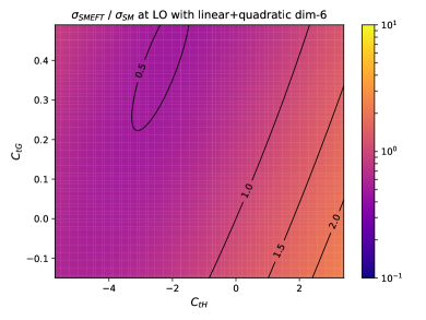
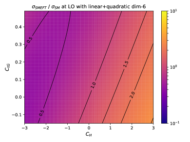
Figure 4: Heat maps showing the dependence of the LO cross section on the pair of Wilson coefficients $C_{tG}$, $C_{tH}$ (left) and $C_{tG}$, $C_{H}$ (right), respectively, with $\Lambda=1$ TeV for the linear dimension-6 truncation. The ranges for $C_{H}$ are oriented at a translation of the limits on $\kappa_{\lambda}$ from Ref. ATLAS:2022jtk , the ranges for the other Wilson coefficients are obtained at ${\cal O}\left(\Lambda^{-2}\right)$ constraints from Ref. Ethier:2021bye (marginalised over the other coefficients). The white areas denote regions in parameter space where the corresponding cross section would be negative.

The allowed ranges of Wilson coefficients are still quite large, such that a sizeable fraction of the 2-dimensional parameter space leads to unphysical negative cross section values. As to be expected, the effect of a variation of $C_{tG}$ within the given range is less pronounced than the one from variations of the leading couplings $C_{tH}$ and $C_{H}$ within their range. From a power counting point of view, the allowed range for $C_{tG}$ should be much smaller, such that the difference of the impact on the cross section would be even more obvious. Nevertheless, it is reasonable to derive bounds while being agnostic about the size of Wilson coefficients as well as considering power counting arguments on the expected impact. The latter is the approach we follow.

In Fig. 5, heat maps for the dependence of the cross section on a variation of (independent) 4-top operator pairs $C_{Qt}^{(1)}$, $C_{Qt}^{(8)}$ and $C_{QQ}^{(1)}+C_{tt}$, $C_{QQ}^{(8)}$ are shown.

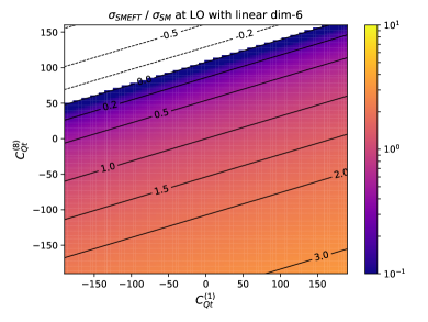
Figure 5: Heat maps showing the dependence of the cross section on the couplings $C_{Qt}^{(1)}$ and $C_{Qt}^{(8)}$ (left) and $C_{QQ}^{(1)}+C_{tt}$ and $C_{QQ}^{(8)}$ (right) with $\Lambda=1$ TeV. The ranges are taken from Ref. Ethier:2021bye based on an ${\cal O}(\Lambda^{-2})$ fit marginalised over the other Wilson coefficients.

Looking at the right plot it is apparent that the $(LL)(LL)$ and $(RR)(RR)$ operators of Ref. Grzadkowski:2010es with coefficients $C_{QQ}^{(1)}$, $C_{tt}$ and $C_{QQ}^{(8)}$ hardly affect the cross section. This can be understood by the very limited contribution to the amplitude, given only by the residual structure ${\cal M}_{\Delta QQ,tt,(8)}^{\text{4-top}}$ in Eq. (21). On the other hand, the $(LL)(RR)$ operators, with coefficients $C_{Qt}^{(1)}$ and $C_{Qt}^{(8)}$, (left plot of Fig. 5) have a large impact on the cross section in the considered range of values, leading to modifications of more than $100\%$ of the LO cross section. The effect on the total cross section of $C_{Qt}^{(8)}$ is stronger than the effect of $C_{Qt}^{(1)}$ (in NDR), which is due to a large impact following from a sign change of the interference with the SM, visible in the upper left diagram of Fig. 9.

Fig. 6 shows the dependence of the LO cross section on the variation of $C_{tG}$ and $C_{Qt}^{(1)}$, comparing the NDR and BMHV scheme choices for the chiral structure of the 4-top operator. We introduce $C_{Qt;\mathrm{BMHV}}^{(1/8)}$ as a short-hand notation to specify that the corresponding amplitude is calculated in the BMHV scheme. Hence, this does not mean that the value of $C_{Qt}^{(1/8)}$ itself is changed by the scheme choice.

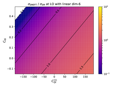
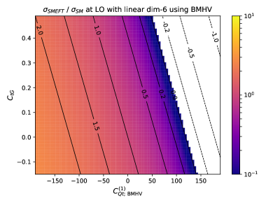
Figure 6: Heat maps demonstrating the effect of the $\gamma_{5}$-scheme choice on the dependence of the cross section on the couplings $C_{tG}$ and $C_{Qt}^{(1)}$ with $\Lambda=1$ TeV. Left plot NDR, right plot BMHV. The ranges are taken from Ref. Ethier:2021bye based on an ${\cal O}(\Lambda^{-2})$ fit marginalised over the other Wilson coefficients.

This selection is an interesting showcase, since in Ref. DiNoi:2023ygk it has been demonstrated that the two Wilson coefficients are closely related, because part of the translation between the schemes is achieved by shifting $C_{tG}$ by contributions that are of equal order in the power counting as the original value of $C_{tG}$, see Eq. (22). The gradient of the cross section in NDR (left) points in a completely different direction than the one in BMHV (right) and also the magnitude of the gradient changes significantly. This demonstrates that bounds set on these operators individually, without considering cancellations of the scheme dependence between different operator contributions, may not be very meaningful.

In Table 3 we present values for the total cross section for the SM and benchmark point 6, using truncation options (a) and (b) at NLO QCD. We also demonstrate their dependence on the variation of a single subleading Wilson coefficient.

BM	SM	6 (a)	6 (b)
$\sigma_{\rm{NLO}}$[fb]	30.9${}^{+14\%}_{-13\%}$	56.5${}^{+22\%}_{-19\%}$	78.7${}^{+18\%}_{-15\%}$
$C_{tG}$
$\scriptsize\begin{aligned} &\left[{0.0085}\right.,&\left.{0.14}\right]\\ &\left[{-0.15}\right.,&\left.{0.49}\right]\end{aligned}$	$\scriptsize\begin{aligned} &\left[{-0.63\%}\right.&\left.{-10\%}\right]\\ &\left[{+11\%}\right.&\left.{-36\%}\right]\end{aligned}$	$\scriptsize\begin{aligned} &\left[{-0.34\%}\right.&\left.{-5.6\%}\right]\\ &\left[{+6.0\%}\right.&\left.{-20\%}\right]\end{aligned}$	$\scriptsize\begin{aligned} &\left[{-0.26\%}\right.&\left.{-4.3\%}\right]\\ &\left[{+4.6\%}\right.&\left.{-15\%}\right]\end{aligned}$
$C_{Qt}^{(1)}$
$\scriptsize\begin{aligned} &\left[{-200}\right.,&\left.{160}\right]\\ &\left[{-190}\right.,&\left.{190}\right]\end{aligned}$	$\scriptsize\begin{aligned} &\left[{-35\%}\right.&\left.{+28\%}\right]\\ &\left[{-34\%}\right.&\left.{+34\%}\right]\end{aligned}$	$\scriptsize\begin{aligned} &\left[{-19\%}\right.&\left.{+15\%}\right]\\ &\left[{-18\%}\right.&\left.{+18\%}\right]\end{aligned}$	$\scriptsize\begin{aligned} &\left[{+31\%}\right.&\left.{-25\%}\right]\\ &\left[{+30\%}\right.&\left.{-30\%}\right]\end{aligned}$
$C_{Qt;\mathrm{BMHV}}^{(1)}$
$\scriptsize\begin{aligned} &\left[{-200}\right.,&\left.{160}\right]\\ &\left[{-190}\right.,&\left.{190}\right]\end{aligned}$	$\scriptsize\begin{aligned} &\left[{+101\%}\right.&\left.{-81\%}\right]\\ &\left[{+96\%}\right.&\left.{-96\%}\right]\end{aligned}$	$\scriptsize\begin{aligned} &\left[{+55\%}\right.&\left.{-44\%}\right]\\ &\left[{+53\%}\right.&\left.{-53\%}\right]\end{aligned}$	$\scriptsize\begin{aligned} &\left[{+88\%}\right.&\left.{-71\%}\right]\\ &\left[{+84\%}\right.&\left.{-84\%}\right]\end{aligned}$
$C_{Qt}^{(8)}$
$\scriptsize\begin{aligned} &\left[{-5.6}\right.,&\left.{20}\right]\\ &\left[{-190}\right.,&\left.{160}\right]\end{aligned}$	$\scriptsize\begin{aligned} &\left[{+3.2\%}\right.&\left.{-11\%}\right]\\ &\left[{+106\%}\right.&\left.{-89\%}\right]\end{aligned}$	$\scriptsize\begin{aligned} &\left[{+1.7\%}\right.&\left.{-6.1\%}\right]\\ &\left[{+58\%}\right.&\left.{-49\%}\right]\end{aligned}$	$\scriptsize\begin{aligned} &\left[{+3.1\%}\right.&\left.{-11\%}\right]\\ &\left[{+105\%}\right.&\left.{-88\%}\right]\end{aligned}$
$C_{Qt;\mathrm{BMHV}}^{(8)}$
$\scriptsize\begin{aligned} &\left[{-5.6}\right.,&\left.{20}\right]\\ &\left[{-190}\right.,&\left.{160}\right]\end{aligned}$	$\scriptsize\begin{aligned} &\left[{+3.8\%}\right.&\left.{-13\%}\right]\\ &\left[{+127\%}\right.&\left.{-107\%}\right]\end{aligned}$	$\scriptsize\begin{aligned} &\left[{+2.1\%}\right.&\left.{-7.3\%}\right]\\ &\left[{+69\%}\right.&\left.{-58\%}\right]\end{aligned}$	$\scriptsize\begin{aligned} &\left[{+3.4\%}\right.&\left.{-12\%}\right]\\ &\left[{+114\%}\right.&\left.{-96\%}\right]\end{aligned}$
$C_{QQ}^{(1)}+C_{tt}$
$\scriptsize\begin{aligned} &\left[{-6.1}\right.,&\left.{23}\right]\\ &\left[{-190}\right.,&\left.{190}\right]\end{aligned}$	$\scriptsize\begin{aligned} &\left[{-0.11\%}\right.&\left.{+0.42\%}\right]\\ &\left[{-3.5\%}\right.&\left.{+3.5\%}\right]\end{aligned}$	$\scriptsize\begin{aligned} &\left[{-0.061\%}\right.&\left.{+0.23\%}\right]\\ &\left[{-1.9\%}\right.&\left.{+1.9\%}\right]\end{aligned}$	$\scriptsize\begin{aligned} &\left[{+0.094\%}\right.&\left.{-0.36\%}\right]\\ &\left[{+2.9\%}\right.&\left.{-2.9\%}\right]\end{aligned}$
$C_{QQ}^{(8)}$
$\scriptsize\begin{aligned} &\left[{-26}\right.,&\left.{58}\right]\\ &\left[{-190}\right.,&\left.{170}\right]\end{aligned}$	$\scriptsize\begin{aligned} &\left[{-0.16\%}\right.&\left.{+0.35\%}\right]\\ &\left[{-1.2\%}\right.&\left.{+1.0\%}\right]\end{aligned}$	$\scriptsize\begin{aligned} &\left[{-0.087\%}\right.&\left.{+0.19\%}\right]\\ &\left[{-0.63\%}\right.&\left.{+0.57\%}\right]\end{aligned}$	$\scriptsize\begin{aligned} &\left[{+0.13\%}\right.&\left.{-0.30\%}\right]\\ &\left[{+0.98\%}\right.&\left.{-0.87\%}\right]\end{aligned}$

Table 3: Total cross sections for Higgs-boson pair production at NLO QCD for the SM and benchmark point 6 using truncation option (a) or (b) at $13.6$ TeV. The modification of the cross section due to a variation of the subleading Wilson coefficients is given as relative change to the base value in the second row. The uncertainties in the second row are scale uncertainties based on 3-point scale variations. The ranges of the subleading Wilson coefficients are oriented at ${\cal O}\left(\Lambda^{-2}\right)$ constraints from Ref. Ethier:2021bye (Upper values: individual bounds, lower values: marginalised over the other coefficients). The effect of the Wilson coefficients $C_{Qt}^{(1)}$ and $C_{Qt}^{(8)}$ is also shown for the BMHV scheme, which is denoted by $C_{Qt;\mathrm{BMHV}}^{(1)}$ and $C_{Qt;\mathrm{BMHV}}^{(8)}$.

In general, the relative difference due to the variation of these Wilson coefficients is more pronounced for the SM cross section than for benchmark point 6.

Due to the asymmetric range of $C_{tG}$, its variation tends to a damping of the cross section, with up to $-36\%$ relative to the SM. For benchmark point 6, truncation (a) leads to a larger relative effect of $C_{tG}$ on the cross section than truncation (b).

The variation of single 4-top Wilson coefficients, on the other hand, is fairly symmetric for the marginalised limits and has larger relative impact for truncation option (b) than for truncation option (a). The cross section difference for a variation of $C_{Qt}^{(1)}$ or $C_{Qt}^{(8)}$ is larger when working in the BMHV scheme than in NDR, and the scheme difference is much more visible for $C_{Qt}^{(1)}$. The $C_{Qt}^{(1)}$ variation leads to up to $\sim 35\%$ effects on the cross section in the NDR scheme and up to $\sim 100\%$ in BMHV, whereas for $C_{Qt}^{(8)}$ the maximum difference is in both schemes $\gtrsim 100\%$. As already indicated by the heat map on the right of Fig. 5, the effect of $C_{QQ}^{(1)}$, $C_{tt}$ and $C_{QQ}^{(8)}$ variation is very small, with a relative difference of less than $4\%$ and being only a fraction of the uncertainty due to 3-point scale variations. The effects of $C_{Qt}^{(1)}$ or $C_{Qt}^{(8)}$ on the difference $\Delta C_{tG}:=C_{tG}^{\text{BMHV}}-C_{tG}$ and $\Delta C_{tH}:=C_{tH}^{\text{BMHV}}-C_{tH}$ are illustrated later at distribution level in Fig. 11.

4.2 Higgs boson pair invariant mass distributions

In this section we present differential distributions depending on the invariant mass of the Higgs boson pair, $m_{hh}$, combining NLO QCD results and subleading operator contributions at LO QCD. Each plot demonstrates the variation of a single subleading Wilson coefficient w.r.t. either the SM or benchmark point 6 for truncations (a) (linear dimension-6 only) and (b) (linear+quadratic dimension-6).

In Fig. 7 the variation of the chromomagnetic operator coefficient $C_{tG}$ in the ranges specified in Table 3 is shown.

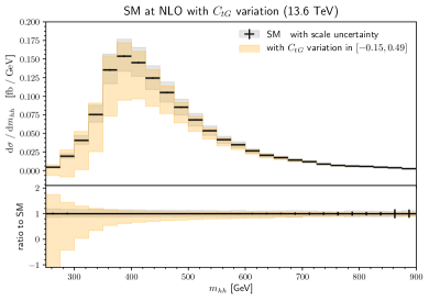
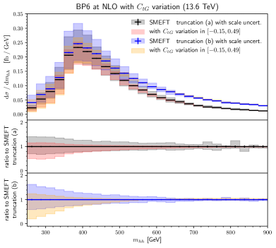
Figure 7: Effects of $C_{tG}$-variations in the corresponding ranges. Left: variation w.r.t. the SM $m_{hh}$-distribution, right: variation w.r.t. benchmark point 6 (BP6) for truncation options (a) and (b).

In the low $m_{hh}$-region, the effects can noticeably exceed the scale uncertainty band. Note that the $C_{tG}$-variation range is asymmetric around zero and that the interference of the $C_{tG}$-term with the SM contribution tends to decrease the cross section.

In Fig. 8 we present the variation of the 4-top operator coefficient $C_{QQ}^{(8)}$ and the combination $C_{QQ}^{(8)}+C_{tt}$.

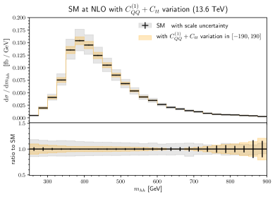
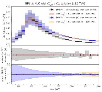
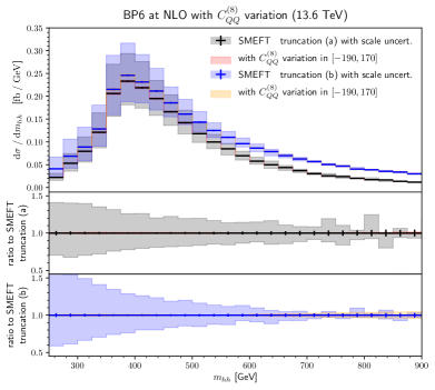
Figure 8: left: $C_{QQ}^{(1)}+C_{tt}$, right: $C_{QQ}^{(8)}$; upper: SM, lower: benchmark point 6.

As observed at the level of total cross sections in Section 4.1, the contribution of these operators remains within the scale uncertainties, except for small deviations in the tails for the case of $C_{QQ}^{(1)}+C_{tt}$. Thus the process $gg\to hh$ is not sensitive to those operators even if the coefficients are varied in ranges as large as $[-190,190]$. The situation is different for the operators $C_{Qt}^{(1)}$ and $C_{Qt}^{(8)}$, as we will show below. However, the contribution of these Wilson coefficients depends on the chosen $\gamma_{5}$-scheme in dimensional regularisation, as explained in Section 2.2.

We begin with Fig. 9 which demonstrates the effect of varying $C_{Qt}^{(1)}$.

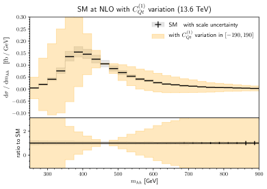
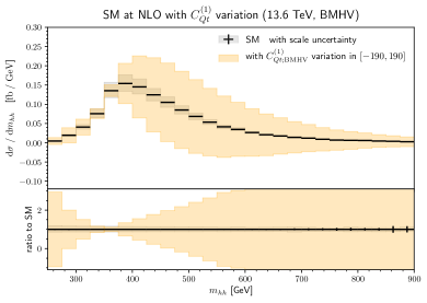
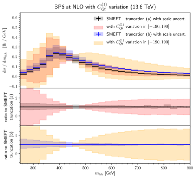
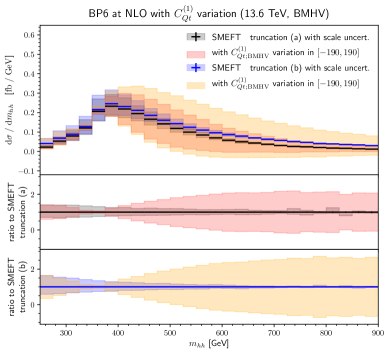
Figure 9: Effects of $C_{Qt}^{(1)}$-variations. Left: NDR, right: BMHV; upper: SM, lower: benchmark point 6.

We observe sizeable effects, differing from the baseline prediction (SM or benchmark 6) by more than $100\%$ for some regions, which also leads to negative cross section values. In NDR, the low- and high $m_{hh}$-regions exhibit large differences beyond the scale uncertainty, with unphysical cross sections at low $m_{hh}$ values and a sign change around $m_{hh}\sim 460$ TeV. This behaviour changes significantly in BMHV: there are visible, but weaker effects in the low $m_{hh}$-region, the sign change occurs around $m_{hh}\sim 360$ TeV and the deviation in the high $m_{hh}$-region begins for lower invariant masses and is also more pronounced.

The scheme dependent behaviour of $C_{Qt}^{(8)}$ is shown in Fig. 10.

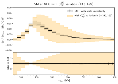
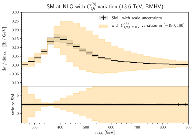
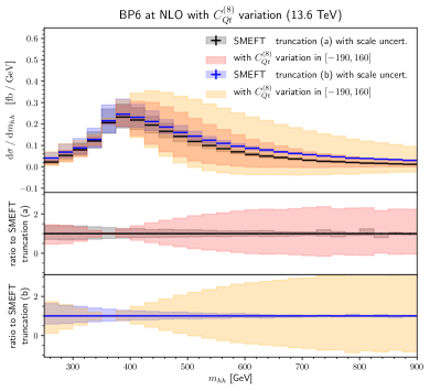
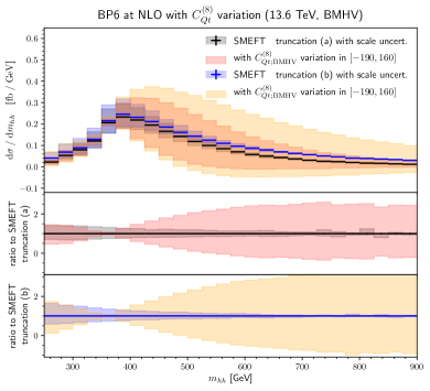
Figure 10: Effects of $C_{Qt}^{(8)}$-variations. Left: NDR, right: BMHV; upper: SM, lower: benchmark point 6.

For both schemes we observe small effects in the low $m_{hh}$-region, a sign change of the contribution around $m_{hh}\sim 360$ TeV and a pronounced effect in the high $m_{hh}$-region. Overall, the difference between the schemes is not as significant as in the case of $C_{Qt}^{(1)}$. The contribution to the $m_{hh}$ distribution in the BMHV scheme (right column of Fig. 10) is qualitatively very similar to the case of $C_{Qt}^{(1)}$ shown in Fig. 9.

In order to better understand the qualitative difference between the $C_{Qt}^{(1)}$ and $C_{Qt}^{(8)}$ variations in NDR, we investigate the effect of those rational terms contributing in NDR which are responsible for the scheme difference and eventually the translation relation Eq. (22). We distinguish in the following between the scheme dependent parts $\Delta C_{tG}:=C_{tG}^{\text{BMHV}}-C_{tG}$, leading to the shift of $C_{tG}$, and $\Delta C_{tH}:=C_{tH}^{\text{BMHV}}-C_{tH}$, leading to the shift of $C_{tH}$. In Fig. 11 we present the difference to the SM $m_{hh}$ distribution originating from those scheme dependent terms, where we individually vary $C_{Qt}^{(1)}$ or $C_{Qt}^{(8)}$, respectively.

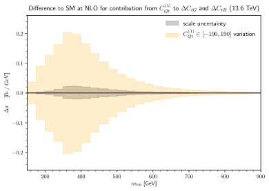
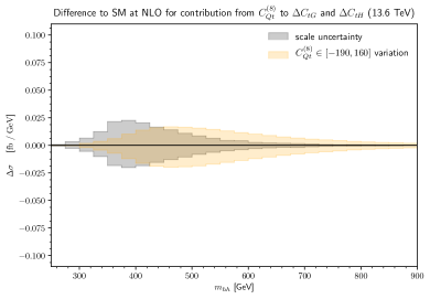
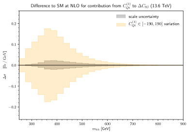
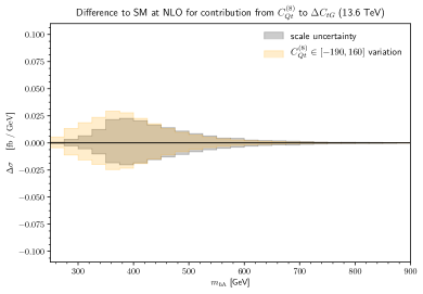
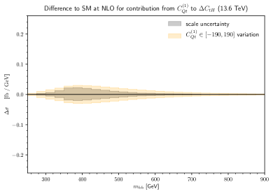
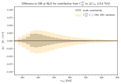
Figure 11: Demonstration of the difference $\Delta\sigma=\frac{d\sigma}{dm_{hh}}-\frac{d\sigma_{\text{SM}}}{dm_{hh}}$ to the SM invariant mass distribution only including contributions of the scheme dependent terms, $\Delta C_{tG}:=C_{tG}^{\text{BMHV}}-C_{tG}$ and $\Delta C_{tH}:=C_{tH}^{\text{BMHV}}-C_{tH}$, for individual variations of $C_{Qt}^{(1)}$ and $C_{Qt}^{(8)}$, respectively. Left: contribution from a $C_{Qt}^{(1)}$ variation, right: contribution from a $C_{Qt}^{(8)}$ variation. Upper: sum of scheme dependent terms ($\Delta C_{tG}$ and $\Delta C_{tH}$), middle: only $\Delta C_{tG}$, lower: only $\Delta C_{tH}$. The gray bands denote the SM 3-point scale uncertainty for reference.

Considering all scheme dependent terms, there is a prominent contribution from $C_{Qt}^{(1)}$, which is much larger than the scale uncertainty of the SM result for the whole $m_{hh}$-range, especially apparent in the low to intermediate $m_{hh}$-regime. Investigating the constituents, we notice that $\Delta C_{tG}$ is much more relevant than $\Delta C_{tH}$ when considering the contributions from $C_{Qt}^{(1)}$ to the shift. Comparing the change on the distribution related to $\Delta C_{tG}$ and $\Delta C_{tH}$ separately (middle and bottom left panels in Fig. 11) to the effect of the sum of both contributions (top left panel in Fig. 11), we observe that the range of the band in the top left panel is given by the sum of the ranges observed for $\Delta C_{tG}$ and $\Delta C_{tH}$ individually. For $C_{Qt}^{(8)}$, the structure of the contributions from the scheme dependent terms is different. Here the effect is larger for the case of $\Delta C_{tH}$ than for $\Delta C_{tG}$, see middle and bottom right panels of Fig. 11. In addition, there is a clear cancellation between individual contributions from $\Delta C_{tG}$ and $\Delta C_{tH}$, as can be seen from the effect on the sum of all rational terms (top right panel of Fig. 11), thus leading to an almost vanishing contribution in the low-$m_{hh}$ region. Comparing the left and right columns of Fig. 11, we observe that the individual shifts due to $C_{Qt}^{(8)}$ versus $C_{Qt}^{(1)}$ behave quite differently. This difference is related to the different colour structures of the relevant scheme dependent terms. On the one hand, the terms contributing to the shift $\Delta C_{tH}$ include a factor of $\Delta C_{tH}\sim\left(C_{Qt}^{(1)}+\frac{4}{3}C_{Qt}^{(8)}\right)$ (inserting explicit $SU(3)_{QCD}$ colour factors), such that the contribution from $C_{Qt}^{(8)}$ is slightly enhanced. The terms contributing to the shift $\Delta C_{tG}$, on the other hand, include a factor of $\Delta C_{tG}\sim\left(C_{Qt}^{(1)}-\frac{1}{6}C_{Qt}^{(8)}\right)$, thus this effect is larger for $C_{Qt}^{(1)}$ and the sign of the contribution from $C_{Qt}^{(8)}$ is opposite to the one from $C_{Qt}^{(1)}$.

We should emphasise again that the observed $\gamma_{5}$-scheme dependence of individual Wilson coefficients does not lead to a scheme dependence of the full amplitude. Both schemes represent equivalent parametrisations of the amplitude and of the renormalisation group flow, the translation has been worked out in Ref. DiNoi:2023ygk . However, fits to constrain these Wilson coefficients should take into account that they are not individually scheme-independent. For example, constraints on $C_{tG}$ either come with a scheme uncertainty or should be derived in combination with $C_{Qt}^{(1)}$ and $C_{Qt}^{(8)}$, calculated in the same scheme.

5 Conclusions

We have calculated the matrix elements including the chromomagnetic operator and 4-top operators contributing to Higgs boson pair production in gluon fusion and demonstrated that these operators both appear at the same subleading order in a power counting scheme that takes into account a tree-loop classification of dimension-6 SMEFT operators. These subleading contributions, entering the cross section at LO QCD, have been combined with the NLO QCD corrections and the dominant SMEFT operators as described in Ref. Heinrich:2022idm , in the form of Eqs. (6)-(8). This combination will be provided as an extension to the public ggHH_SMEFT code as part of the POWHEG-Box-V2. We have also described the usage of the new features.

The matrix elements of the 4-top contributions have been decomposed analogous to the case of $gg\to h$ described in Refs. Alasfar:2022zyr ; DiNoi:2023ygk . In particular, the parts depending on the $\gamma_{5}$-scheme in dimensional regularisation have been identified, such that we found a similar scheme dependence as in the $gg\to h$ case, which can be understood as a finite shift of Wilson coefficients, see Eq. (22) and Ref. DiNoi:2023ygk .

The effect of the subleading operators on the total cross section and on the Higgs boson pair invariant mass distribution has been studied in detail, both with respect to the SM and for benchmark point 6. We observed that the operators $\mathcal{O}_{QQ}^{(1)}$, $\mathcal{O}_{tt}$ and $\mathcal{O}_{QQ}^{(8)}$ only marginally contribute, therefore $gg\to hh$ is not an adequate process to probe those coefficients. The cross section is noticeably affected by a variation of the Wilson coefficient $C_{tG}$ within current conservative bounds, which can lead to a damping of the invariant mass distribution in the low to intermediate $m_{hh}$–region. However, the highest sensitivity is observed by a variation of $C_{Qt}^{(1)}$ and $C_{Qt}^{(8)}$ within current bounds.

As has been investigated for single Higgs production in Ref. DiNoi:2023ygk and confirmed in this work, those Wilson coefficients are precisely the ones which, when considered individually, depend on the chosen $\gamma_{5}$-scheme. Therefore, bounds for individual coefficients can turn out to be significantly different due to a (more or less arbitrary) calculational scheme choice, which makes their interpretation difficult. This does not only hold for the above-mentioned 4-top operators, but also for the Wilson coefficient $C_{tG}$, which, at the same order in the power counting, can contain a contribution from $C_{Qt}^{(1)}$ and $C_{Qt}^{(8)}$, depending on the scheme choice. Inserting numerical values for current bounds on these Wilson coefficients Ethier:2021bye into Eq. (22) illustrates that the shift induced by a scheme change can even be larger than the interval given by the original bounds. To obtain more meaningful results, it is therefore recommended to study those Wilson coefficients which are connected through the scheme translation relations together, such that their combination is a scheme independent parametrisation of BSM physics at the studied order in the power counting.

In the future it would be desirable to have QCD corrections to those subleading operators as well, in order to compare on equal footing with the leading operators, at NLO QCD. However, including NLO corrections to the 4-top operators would require a 3-loop calculation involving Higgs and top-quark masses and therefore would be clearly beyond the scope of this paper. Furthermore, operators of the class $\psi^{2}\phi^{2}D$ have not been considered in this work, even though they would enter at the same power counting order, because they are considered as electroweak-type. However, this indicates that the strict separation between QCD and electroweak contributions becomes ambiguous once SMEFT operators beyond the leading contributions are included and combined with higher order corrections.

Finally, we note that renormalisation group running effects have not been included in the present study, even though they may lead to sizeable effects. This is left to upcoming work.

References

• (1) S. Weinberg, Phenomenological Lagrangians, Physica A 96 (1979) 327.
• (2) W. Buchmüller and D. Wyler, Effective Lagrangian Analysis of New Interactions and Flavor Conservation, Nucl. Phys. B 268 (1986) 621.
• (3) G. Isidori, F. Wilsch and D. Wyler, The Standard Model effective field theory at work, 2303.16922.
• (4) B. Grzadkowski, M. Iskrzynski, M. Misiak and J. Rosiek, Dimension-Six Terms in the Standard Model Lagrangian, JHEP 10 (2010) 085 [1008.4884].
• (5) I. Brivio and M. Trott, The Standard Model as an Effective Field Theory, Phys. Rept. 793 (2019) 1 [1706.08945].
• (6) K. Mimasu, V. Sanz and C. Williams, Higher Order QCD predictions for Associated Higgs production with anomalous couplings to gauge bosons, JHEP 08 (2016) 039 [1512.02572].
• (7) S. Alioli, W. Dekens, M. Girard and E. Mereghetti, NLO QCD corrections to SM-EFT dilepton and electroweak Higgs boson production, matched to parton shower in POWHEG, JHEP 08 (2018) 205 [1804.07407].
• (8) C. Degrande, G. Durieux, F. Maltoni, K. Mimasu, E. Vryonidou and C. Zhang, Automated one-loop computations in the standard model effective field theory, Phys. Rev. D 103 (2021) 096024 [2008.11743].
• (9) J. Baglio, S. Dawson, S. Homiller, S. D. Lane and I. M. Lewis, Validity of standard model EFT studies of VH and VV production at NLO, Phys. Rev. D 101 (2020) 115004 [2003.07862].
• (10) M. Battaglia, M. Grazzini, M. Spira and M. Wiesemann, Sensitivity to BSM effects in the Higgs pT spectrum within SMEFT, JHEP 11 (2021) 173 [2109.02987].
• (11) S. Dawson and P. P. Giardino, New physics through Drell-Yan standard model EFT measurements at NLO, Phys. Rev. D 104 (2021) 073004 [2105.05852].
• (12) I. Brivio, SMEFT calculations for the LHC, PoS LHCP2021 (2021) 078.
• (13) G. Heinrich, J. Lang and L. Scyboz, SMEFT predictions for $gg\to hh$ at full NLO QCD and truncation uncertainties, JHEP 08 (2022) 079 [2204.13045].
• (14) G. Buchalla, M. Höfer and C. Müller-Salditt, $h\to gg$ and $h\to\gamma\gamma$ with anomalous couplings at next-to-leading order in QCD, Phys. Rev. D 107 (2023) 076021 [2212.08560].
• (15) E. E. Jenkins, A. V. Manohar and M. Trott, Renormalization Group Evolution of the Standard Model Dimension Six Operators I: Formalism and lambda Dependence, JHEP 10 (2013) 087 [1308.2627].
• (16) E. E. Jenkins, A. V. Manohar and M. Trott, Renormalization Group Evolution of the Standard Model Dimension Six Operators II: Yukawa Dependence, JHEP 01 (2014) 035 [1310.4838].
• (17) R. Alonso, E. E. Jenkins, A. V. Manohar and M. Trott, Renormalization Group Evolution of the Standard Model Dimension Six Operators III: Gauge Coupling Dependence and Phenomenology, JHEP 04 (2014) 159 [1312.2014].
• (18) R. Aoude, F. Maltoni, O. Mattelaer, C. Severi and E. Vryonidou, Renormalisation group effects on SMEFT interpretations of LHC data, 2212.05067.
• (19) M. Chala and J. Santiago, Positivity bounds in the standard model effective field theory beyond tree level, Phys. Rev. D 105 (2022) L111901 [2110.01624].
• (20) S. Dawson et al., LHC EFT WG Note: Precision matching of microscopic physics to the Standard Model Effective Field Theory (SMEFT), 2212.02905.
• (21) J. Aebischer, J. Kumar and D. M. Straub, Wilson: a Python package for the running and matching of Wilson coefficients above and below the electroweak scale, Eur. Phys. J. C 78 (2018) 1026 [1804.05033].
• (22) J. Fuentes-Martin, P. Ruiz-Femenia, A. Vicente and J. Virto, DsixTools 2.0: The Effective Field Theory Toolkit, Eur. Phys. J. C 81 (2021) 167 [2010.16341].
• (23) S. Di Noi and L. Silvestrini, RGESolver: a C++ library to perform renormalization group evolution in the Standard Model Effective Theory, Eur. Phys. J. C 83 (2023) 200 [2210.06838].
• (24) J. Fuentes-Martín, M. König, J. Pagès, A. E. Thomsen and F. Wilsch, A proof of concept for matchete: an automated tool for matching effective theories, Eur. Phys. J. C 83 (2023) 662 [2212.04510].
• (25) C. S. Machado, S. Renner and D. Sutherland, Building blocks of the flavourful SMEFT RG, JHEP 03 (2023) 226 [2210.09316].
• (26) A. Martin and M. Trott, More accurate $\sigma(\mathcal{G}\,\mathcal{G}\rightarrow h)$, $\Gamma(h\rightarrow\mathcal{G}\,\mathcal{G},\mathcal{A}\mathcal{A},\bar{\Psi}{\Psi})$ and Higgs width results via the geoSMEFT, 2305.05879.
• (27) A. Dedes, J. Rosiek, M. Ryczkowski, K. Suxho and L. Trifyllis, SmeftFR v3 – Feynman rules generator for the Standard Model Effective Field Theory, Comput. Phys. Commun. 294 (2024) 108943 [2302.01353].
• (28) J. ter Hoeve, G. Magni, J. Rojo, A. N. Rossia and E. Vryonidou, The automation of SMEFT-Assisted Constraints on UV-Complete Models, 2309.04523.
• (29) S. Dawson, S. Homiller and M. Sullivan, Impact of dimension-eight SMEFT contributions: A case study, Phys. Rev. D 104 (2021) 115013 [2110.06929].
• (30) J. Ellis, H.-J. He and R.-Q. Xiao, Probing neutral triple gauge couplings at the LHC and future hadron colliders, Phys. Rev. D 107 (2023) 035005 [2206.11676].
• (31) S. Alioli et al., Theoretical developments in the SMEFT at dimension-8 and beyond, in Snowmass 2021, 3, 2022, 2203.06771.
• (32) R. Gomez Ambrosio, J. ter Hoeve, M. Madigan, J. Rojo and V. Sanz, Unbinned multivariate observables for global SMEFT analyses from machine learning, JHEP 03 (2023) 033 [2211.02058].
• (33) L. Allwicher, D. A. Faroughy, F. Jaffredo, O. Sumensari and F. Wilsch, Drell-Yan tails beyond the Standard Model, JHEP 03 (2023) 064 [2207.10714].
• (34) K. Asteriadis, S. Dawson and D. Fontes, Double insertions of SMEFT operators in gluon fusion Higgs boson production, Phys. Rev. D 107 (2023) 055038 [2212.03258].
• (35) S. Borowka, N. Greiner, G. Heinrich, S. P. Jones, M. Kerner, J. Schlenk et al., Higgs Boson Pair Production in Gluon Fusion at Next-to-Leading Order with Full Top-Quark Mass Dependence, Phys. Rev. Lett. 117 (2016) 012001 [1604.06447].
• (36) S. Borowka, N. Greiner, G. Heinrich, S. P. Jones, M. Kerner, J. Schlenk et al., Full top quark mass dependence in Higgs boson pair production at NLO, JHEP 10 (2016) 107 [1608.04798].
• (37) J. Baglio, F. Campanario, S. Glaus, M. Mühlleitner, M. Spira and J. Streicher, Gluon fusion into Higgs pairs at NLO QCD and the top mass scheme, Eur. Phys. J. C 79 (2019) 459 [1811.05692].
• (38) J. Baglio, F. Campanario, S. Glaus, M. Mühlleitner, J. Ronca, M. Spira et al., Higgs-Pair Production via Gluon Fusion at Hadron Colliders: NLO QCD Corrections, JHEP 04 (2020) 181 [2003.03227].
• (39) P. Nason, A New method for combining NLO QCD with shower Monte Carlo algorithms, JHEP 11 (2004) 040 [hep-ph/0409146].
• (40) S. Frixione, P. Nason and C. Oleari, Matching NLO QCD computations with Parton Shower simulations: the POWHEG method, JHEP 11 (2007) 070 [0709.2092].
• (41) S. Alioli, P. Nason, C. Oleari and E. Re, A general framework for implementing NLO calculations in shower Monte Carlo programs: the POWHEG BOX, JHEP 06 (2010) 043 [1002.2581].
• (42) G. Heinrich, S. P. Jones, M. Kerner, G. Luisoni and E. Vryonidou, NLO predictions for Higgs boson pair production with full top quark mass dependence matched to parton showers, JHEP 08 (2017) 088 [1703.09252].
• (43) G. Heinrich, S. P. Jones, M. Kerner, G. Luisoni and L. Scyboz, Probing the trilinear Higgs boson coupling in di-Higgs production at NLO QCD including parton shower effects, JHEP 06 (2019) 066 [1903.08137].
• (44) G. Buchalla, M. Capozi, A. Celis, G. Heinrich and L. Scyboz, Higgs boson pair production in non-linear Effective Field Theory with full $m_{t}$-dependence at NLO QCD, JHEP 09 (2018) 057 [1806.05162].
• (45) G. Heinrich, S. P. Jones, M. Kerner and L. Scyboz, A non-linear EFT description of $gg\to HH$ at NLO interfaced to POWHEG, JHEP 10 (2020) 021 [2006.16877].
• (46) E. Bagnaschi, G. Degrassi and R. Gröber, Higgs boson pair production at NLO in the Powheg approach and the top quark mass uncertainties, Eur. Phys. J. C 83 (2023) 1054 [2309.10525].
• (47) D. de Florian, I. Fabre and J. Mazzitelli, Higgs boson pair production at NNLO in QCD including dimension 6 operators, JHEP 10 (2017) 215 [1704.05700].
• (48) R. Gröber, M. Mühlleitner, M. Spira and J. Streicher, NLO QCD Corrections to Higgs Pair Production including Dimension-6 Operators, JHEP 09 (2015) 092 [1504.06577].
• (49) R. Gröber, M. Mühlleitner and M. Spira, Higgs Pair Production at NLO QCD for CP-violating Higgs Sectors, Nucl. Phys. B 925 (2017) 1 [1705.05314].
• (50) D. de Florian, I. Fabre, G. Heinrich, J. Mazzitelli and L. Scyboz, Anomalous couplings in Higgs-boson pair production at approximate NNLO QCD, JHEP 09 (2021) 161 [2106.14050].
• (51) J. Davies, K. Schönwald, M. Steinhauser and H. Zhang, Next-to-leading order electroweak corrections to $gg\to HH$ and $gg\to gH$ in the large-mt limit, JHEP 10 (2023) 033 [2308.01355].
• (52) J. Davies, G. Mishima, K. Schönwald, M. Steinhauser and H. Zhang, Higgs boson contribution to the leading two-loop Yukawa corrections to $gg\to HH$, JHEP 08 (2022) 259 [2207.02587].
• (53) M. Mühlleitner, J. Schlenk and M. Spira, Top-Yukawa-induced corrections to Higgs pair production, JHEP 10 (2022) 185 [2207.02524].
• (54) S. Di Noi, R. Gröber, G. Heinrich, J. Lang and M. Vitti, On $\gamma_{5}$ schemes and the interplay of SMEFT operators in the Higgs-gluon coupling, 2310.18221.
• (55) T. Corbett, A. Martin and M. Trott, Consistent higher order $\sigma\left(\mathcal{GG}\to h\right)$, $\Gamma\left(h\to\mathcal{GG}\right)$ and $\Gamma(h\to\gamma\gamma)$ in geoSMEFT, JHEP 12 (2021) 147 [2107.07470].
• (56) J. Aebischer, M. Pesut and Z. Polonsky, Renormalization scheme factorization of one-loop Fierz identities, 2306.16449.
• (57) A. Greljo, A. Palavrić and A. E. Thomsen, Adding Flavor to the SMEFT, JHEP 10 (2022) 010 [2203.09561].
• (58) SMEFiT collaboration, J. J. Ethier, G. Magni, F. Maltoni, L. Mantani, E. R. Nocera, J. Rojo et al., Combined SMEFT interpretation of Higgs, diboson, and top quark data from the LHC, JHEP 11 (2021) 089 [2105.00006].
• (59) G. D’Ambrosio, G. F. Giudice, G. Isidori and A. Strumia, Minimal flavor violation: An Effective field theory approach, Nucl. Phys. B 645 (2002) 155 [hep-ph/0207036].
• (60) N. D. Christensen and C. Duhr, FeynRules - Feynman rules made easy, Comput. Phys. Commun. 180 (2009) 1614 [0806.4194].
• (61) A. Alloul, N. D. Christensen, C. Degrande, C. Duhr and B. Fuks, FeynRules 2.0 - A complete toolbox for tree-level phenomenology, Comput. Phys. Commun. 185 (2014) 2250 [1310.1921].
• (62) C. Degrande, C. Duhr, B. Fuks, D. Grellscheid, O. Mattelaer and T. Reiter, UFO - The Universal FeynRules Output, Comput. Phys. Commun. 183 (2012) 1201 [1108.2040].
• (63) L. Darmé et al., UFO 2.0: the ‘Universal Feynman Output’ format, Eur. Phys. J. C 83 (2023) 631 [2304.09883].
• (64) D. Barducci et al., Interpreting top-quark LHC measurements in the standard-model effective field theory, 1802.07237.
• (65) C. Arzt, M. B. Einhorn and J. Wudka, Patterns of deviation from the standard model, Nucl. Phys. B 433 (1995) 41 [hep-ph/9405214].
• (66) G. Buchalla, G. Heinrich, C. Müller-Salditt and F. Pandler, Loop counting matters in SMEFT, SciPost Phys. 15 (2023) 088 [2204.11808].
• (67) M. Trott, Methodology for theory uncertainties in the standard model effective field theory, Phys. Rev. D 104 (2021) 095023 [2106.13794].
• (68) G. Guedes, P. Olgoso and J. Santiago, Towards the one loop IR/UV dictionary in the SMEFT: one loop generated operators from new scalars and fermions, 2303.16965.
• (69) P. Nogueira, Automatic Feynman graph generation, J. Comput. Phys. 105 (1993) 279.
• (70) V. Shtabovenko, R. Mertig and F. Orellana, FeynCalc 9.3: New features and improvements, Comput. Phys. Commun. 256 (2020) 107478 [2001.04407].
• (71) V. Shtabovenko, R. Mertig and F. Orellana, New Developments in FeynCalc 9.0, Comput. Phys. Commun. 207 (2016) 432 [1601.01167].
• (72) R. Mertig, M. Bohm and A. Denner, FEYN CALC: Computer algebraic calculation of Feynman amplitudes, Comput. Phys. Commun. 64 (1991) 345.
• (73) GoSam collaboration, G. Cullen et al., G$\scriptsize{O}$S$\scriptsize{AM}$-2.0: a tool for automated one-loop calculations within the Standard Model and beyond, Eur. Phys. J. C 74 (2014) 3001 [1404.7096].
• (74) G. Cullen, N. Greiner, G. Heinrich, G. Luisoni, P. Mastrolia, G. Ossola et al., Automated One-Loop Calculations with GoSam, Eur. Phys. J. C 72 (2012) 1889 [1111.2034].
• (75) Magerya, Vitaly, https://magv.github.io/alibrary/alibrary.html, .
• (76) J. Klappert, F. Lange, P. Maierhöfer and J. Usovitsch, Integral reduction with Kira 2.0 and finite field methods, Comput. Phys. Commun. 266 (2021) 108024 [2008.06494].
• (77) P. Maierhöfer, J. Usovitsch and P. Uwer, Kira—A Feynman integral reduction program, Comput. Phys. Commun. 230 (2018) 99 [1705.05610].
• (78) G. Heinrich, S. Jahn, S. P. Jones, M. Kerner, F. Langer, V. Magerya et al., Expansion by regions with pySecDec, Comput. Phys. Commun. 273 (2022) 108267 [2108.10807].
• (79) S. Borowka, G. Heinrich, S. Jahn, S. P. Jones, M. Kerner and J. Schlenk, A GPU compatible quasi-Monte Carlo integrator interfaced to pySecDec, Comput. Phys. Commun. 240 (2019) 120 [1811.11720].
• (80) S. Borowka, G. Heinrich, S. Jahn, S. P. Jones, M. Kerner, J. Schlenk et al., pySecDec: a toolbox for the numerical evaluation of multi-scale integrals, Comput. Phys. Commun. 222 (2018) 313 [1703.09692].
• (81) M. S. Chanowitz, M. Furman and I. Hinchliffe, The Axial Current in Dimensional Regularization, Nucl. Phys. B 159 (1979) 225.
• (82) G. Passarino and M. J. G. Veltman, One Loop Corrections for e+ e- Annihilation Into mu+ mu- in the Weinberg Model, Nucl. Phys. B 160 (1979) 151.
• (83) G. ’t Hooft and M. J. G. Veltman, Scalar One Loop Integrals, Nucl. Phys. B 153 (1979) 365.
• (84) G. ’t Hooft and M. J. G. Veltman, Regularization and Renormalization of Gauge Fields, Nucl. Phys. B 44 (1972) 189.
• (85) P. Breitenlohner and D. Maison, Dimensional Renormalization and the Action Principle, Commun. Math. Phys. 52 (1977) 11.
• (86) N. Deutschmann, C. Duhr, F. Maltoni and E. Vryonidou, Gluon-fusion Higgs production in the Standard Model Effective Field Theory, JHEP 12 (2017) 063 [1708.00460].
• (87) L. Alasfar, J. de Blas and R. Gröber, Higgs probes of top quark contact interactions and their interplay with the Higgs self-coupling, JHEP 05 (2022) 111 [2202.02333].
• (88) T. Hahn and M. Perez-Victoria, Automatized one loop calculations in four-dimensions and D-dimensions, Comput. Phys. Commun. 118 (1999) 153 [hep-ph/9807565].
• (89) J. Butterworth et al., PDF4LHC recommendations for LHC Run II, J. Phys. G43 (2016) 023001 [1510.03865].
• (90) A. Buckley, J. Ferrando, S. Lloyd, K. Nordström, B. Page, M. Rüfenacht et al., LHAPDF6: parton density access in the LHC precision era, Eur. Phys. J. C75 (2015) 132 [1412.7420].
• (91) M. Cacciari, G. P. Salam and G. Soyez, The anti-$k_{T}$ jet clustering algorithm, JHEP 04 (2008) 063 [0802.1189].
• (92) M. Cacciari and G. P. Salam, Dispelling the $N^{3}$ myth for the $k_{t}$ jet-finder, Phys.Lett. B641 (2006) 57 [hep-ph/0512210].
• (93) M. Cacciari, G. P. Salam and G. Soyez, FastJet User Manual, Eur.Phys.J. C72 (2012) 1896 [1111.6097].
• (94) L. Alasfar et al., Effective Field Theory descriptions of Higgs boson pair production, 2304.01968.
• (95) M. Capozi and G. Heinrich, Exploring anomalous couplings in Higgs boson pair production through shape analysis, JHEP 03 (2020) 091 [1908.08923].
• (96) ATLAS collaboration, G. Aad et al., Constraints on the Higgs boson self-coupling from single- and double-Higgs production with the ATLAS detector using pp collisions at s=13 TeV, Phys. Lett. B 843 (2023) 137745 [2211.01216].