Phase Behavior of the Patchy Colloids Confined in the Patchy Porous Media

Abstract

A simple model for functionalized disordered porous media is proposed and the effects of confinement on self-association, percolation and phase behavior of a fluid of patchy particles are studied. The media is formed by a randomly distributed hard-sphere obstacles fixed in space and decorated by a certain number of off-center square-well sites. The properties of the fluid of patchy particles, represented by the fluid of hard spheres each bearing a set of the off-center square-well sites, are studied using an appropriate combination of the scaled particle theory for the porous media, Wertheim’s thermodynamic perturbation theory, and the Flory–Stockmayer theory. To assess the accuracy of the theory a set of computer simulations have been performed. In general, predictions of the theory appear to be in a good agreement with computer simulation results. Confinement and competition between the formation of bonds connecting the fluid particles, and connecting fluid particles and obstacles of the matrix, give rise to a re-entrant phase behavior with three critical points and two separate regions of the liquid-gas phase coexistence.

1 Introduction

Porous materials, both natural (e.g., zeolites, biological tissues, rocks and soil) and artificial (e.g., ceramics, synthetic zeolites, cement, silica aerogels), are ubiquitous. They are relevant for a broad range of applications, e.g., catalysis and sensing, gas storage and separation, adsorption, drug delivery, biomaterial immobilization, environmental remediation, molecular recognition, energy storage, etc ^{1, 2, 3, 4, 5, 6, 7, 8, 9, 10, 11, 12, 13, 14, 15, 16, 17, 18, 19, 20, 21, 22, 23, 24, 25, 26, 27, 28}. In most of the earlier applications of porous materials, conventional porous materials, such as zeolites, silica aerogels or activated carbon, were used ^{29, 30, 31, 32, 33, 34, 35}. Due to the emergence of new classes of porous material, which include metal-organic frameworks  ^{36, 37, 38, 39, 40}, porous organosilicas ^{41, 42}, porous polymers ^{43, 44, 45, 46, 47, 48} and covalent organic frameworks ^{48, 49, 50}, substantial advances in the field were achieved during the last few decades. In particular, due to their well-developed porosity and tunable surface chemistry these composite organic-inorganic porous materials can be relatively easy functionalized, i.e. the properties of the inner surface of the pores can be appropriately modified by decorating it with different functional groups, organic and inorganic moieties, etc. Functionalized porous materials offer a number of new opportunities to achieve desirable properties for a diverse range of industrial applications ⁵¹ and thus detailed and deep understanding of the mechanisms and effects of confinement on the properties of the fluids adsorbed in the porous media is essential for their development.

Over the past several decades substantial progress in the theoretical description of fluids adsorbed in disordered porous media has been achieved ^{52, 53, 54, 55, 56, 57}. Most of the theoretical studies are based on the application of the approach developed by Madden and Glandt ^{58, 59} and Given and Stell ⁶⁰. In these studies a porous medium is modeled as a quenched disordered configuration of the particles and the properties of the fluid adsorbed in a media are described using the so-called replica Ornstein-Zernike (ROZ) theory ^{58, 59, 60}. Subsequently the theory was extended and applied to study the properties of a number of different fluids confined in the porous media, including site-site fluids ^{61, 62, 63}, associating fluids ^{64, 65, 66, 67, 68, 69}, fluids with Coulomb interactions ^{70, 71, 72, 73, 74} and inhomogeneous systems ^{75, 76}. ROZ theory appears to be very useful and is able to provide relatively accurate predictions for the structure and thermodynamic properties of the fluid adsorbed in disordered porous media. However, solution of ROZ equation requires application of numerical methods, i.e. none of ROZ closures proposed so far are amenable to an analytical solution. In addition, straightforward application of the ROZ approach for phase equilibrium calculations is limited by the absence of a convergent solution to the ROZ equation in a relatively large region of thermodynamic states. Recently, a theoretical approach enabling one to analytically describe the properties of hard-sphere fluid adsorbed in the hard-sphere matrix, formed by the fluid of hard spheres quenched at equilibrium, has been developed ^{77, 78, 79, 54, 80, 81}. The theory is based on the appropriate extension of scaled particle theory ⁸². The hard-sphere fluid is routinely used as a reference system in a number of thermodynamic perturbation theories. In particular, a fluid of hard spheres confined in the hard-sphere matrix was used as a reference system in the framework of the Barker-Henderson perturbation theory ^{83, 84}, high-temperature approximation ⁸⁵, Wertheim’s thermodynamic perturbation theory (TPT) ^{81, 86, 87, 88, 89}, associative mean spherical approximation ^{90, 91, 92, 93} and collective variable method ^{94, 95, 96}.

In the current paper we propose a simple model for functionalized disordered porous media and study the effects of confinement on the clusterization, percolation and phase behavior of a fluid of patchy particles. The media is represented by the disordered matrix of the hard-sphere obstacles bearing a certain number of off-center square-well sites (patches). Due to strong, short-range attraction between patches, the obstacles can bond to fluid particles, as well as the fluid particles having the ability to form a network. The theoretical description is carried out combining SPT for the porous media ^{79, 54, 80, 81} and Wertheim’s TPT for associating fluids ^{97, 98, 99}. To assess the accuracy of the theory proposed we generate a set of computer simulation data and compare them against our theoretical predictions.

The paper is organized as follows. In Section 2 we describe the interaction potential model and present the theory. In Section 3 we briefly describe details of the computer simulations. Section 4 contains results and their discussion. Our conclusions are collected in Section 5.

Figure 1: Models of a particle with one, two, three and four patches.

2 The Model and Theory

Patchy colloids are modeled as a one-component hard-sphere fluid with the particles decorated by the set of $n_{1}$ square-well bonding sites (patches) located on the surface Fig. 1. The fluid is confined in the porous media represented by the matrix of the patchy hard-sphere obstacles, quenched at hard-sphere fluid equilibrium Fig. 2. Each of the obstacles has on its surface $n_{0}$ square-well bonding sites (patches). The pair potential $U_{ij}(12)$, which describes the interaction between colloidal particles and between colloidal particles and obstacles is given by

$$U_{ij}(12)=U_{ij}^{(hs)}(r)+\sum_{KL}U_{i_{K}j_{L}}^{(as)}(12),$$ (1)

where

$$U^{(as)}_{i_{K}j_{L}}(12)=U^{(as)}_{i_{K}j_{L}}(z_{12})=\left\{\begin{array}[]{rl}-\epsilon_{ij},&{\rm for}\;z_{12}\leq\omega_{ij}\\ 0,&{\rm otherwise}\end{array}\right.,$$ (2)

$1$ and $2$ stand for the position and orientation of the particles 1 and 2, the indices $i,j$ take the values $(i,j)=(1,1),(1.0),(0,1)$ and denote either fluid particles ($i=1$) or matrix obstacles ($i=0$), the indices $K$ and $L$ denote patches and take the values $A,B,C,\ldots$. $U^{(hs)}_{ij}(r)$ is the hard-sphere potential between the particles of the sizes $\sigma_{i}$ and $\sigma_{j}$, $z_{12}$ is the distance between corresponding sites, $\epsilon_{ij}$ and $\omega_{ij}$ are the depth and width of the square-well potential. Note that $\epsilon_{ij}$ and $\omega_{ij}$ are independent of the type of the patches.

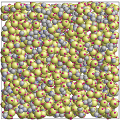
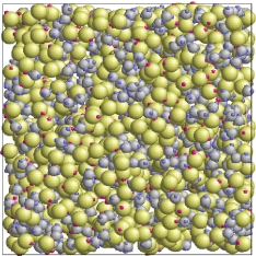
Figure 2: Models of a patchy fluid in a patchy matrix: one-patch fluid in four-patch matrix L1M4 (left panel) and three-patch fluid in one-patch matrix L3M1 (right panel). The fluid particles are represented by the gray spheres and matrix obstacles are shown as the green spheres.

The properties of the model are calculated combining Wertheim’s thermodynamic perturbation theory (TPT) for associating fluids ^{97, 98, 99} and scaled particle theory (SPT), extended to describe a hard-sphere fluid adsorbed in the hard-sphere matrix ^{79, 54, 80}. According to Wertheim’s TPT Helmholtz free energy of the system $A$ can be written in the following form

$$A=A_{ref}+\Delta A_{as},$$ (3)

where $A_{ref}$ is Helmholtz free energy of the reference system, and

$$\frac{\beta\Delta A_{as}}{V}=\rho_{1}n_{1}\left(\ln{X_{1}}-\frac{1}{2}X_{1}+\frac{1}{2}\right)+\rho_{0}n_{0}\left(\ln{X_{0}}-\frac{1}{2}X_{0}+\frac{1}{2}\right),$$ (4)

$\rho_{i}$ is the number density of the particles of the type $i$, $\beta=1/(k_{B}T)$, $k_{B}$ is the Boltzmann constant, $T$ is the temperature, $X_{i}=X_{i_{K}}$ is fraction of the particles with attractive site of type $K$, which belong to the particles of the type $i$, non-bonded. Note that all the patches, which belong to the particles of the type $i$, are equivalent (2). Here $X_{i}$ is obtained from the solution of the following set of equations ^{81 97, 99}

$$4\pi X_{1}\left(\rho_{1}\sigma_{11}^{3}n_{1}X_{1}T_{11}^{(as)}g_{11}^{(ref)}+\rho_{0}\sigma_{01}^{3}n_{0}X_{0}T_{01}^{(as)}g_{01}^{(ref)}\right)+X_{1}-1=0,$$ (5)

and

$$4\pi X_{0}\rho_{1}\sigma_{01}^{3}n_{1}X_{1}T_{01}^{(as)}g_{01}^{(ref)}+X_{0}-1=0,$$ (6)

where $\sigma_{ij}=(\sigma_{i}+\sigma_{j})/2$, $g_{ij}^{(ref)}$ is the contact value of the radial distribution function of the reference system,

$$\sigma_{ij}^{3}T_{ij}^{(as)}=\int_{\sigma_{ij}}^{\sigma_{ij}+\omega_{ij}}{\tilde{f}}_{ij}^{(as)}(r)r^{2}dr,$$ (7)

and ${\tilde{f}}^{(as)}_{ij}(r)$ is the orientationally averaged Mayer function for square-well site-site potential

$${\tilde{f}}^{(as)}_{ij}(r)=\left(e^{\beta\epsilon_{ij}}-1\right)\left(\omega_{ij}+\sigma_{ij}-r\right)^{2}\left(2\omega_{ij}-\sigma_{ij}+r\right)/\left(6\sigma_{i}\sigma_{j}r\right)$$ (8)

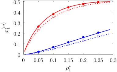
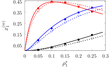
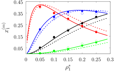
Figure 3: Fraction of $m$ times bonded fluid particles $x_{1}^{(m)}$ as a function of the fluid density $\rho_{1}^{*}=\rho_{1}\sigma_{1}^{3}$ for the model $L2M0$ (top panel), $L3M0$ (intermediate panel), $L4M0$ (bottom panel) at different values of the $\eta_{0}$, i.e. $\eta_{0}=0.1$ (dashed lines and open circles) and $\eta_{0}=0.2$ (solid lines and filled circles). Here $m=1$ (red curves and symbols), $m=2$ (blue lines and symbols), $m=3$ (black lines and symbols), $m=4$ (green line and symbols). Theoretical results are represented by the lines and computer simulation results by the symbols.

The chemical potential, $\mu$, and pressure, $P$, of the system are calculated using standard thermodynamic relations, i.e.

$$\mu=\mu_{ref}+\Delta\mu_{as},\;\;\;\;\;\;\;P=P_{ref}+\Delta P_{as},$$ (9)

and are used for the phase equilibrium calculations. Here

$$\Delta\mu_{as}=\left({\partial(\Delta A_{as}/V)\over\partial\rho_{1}}\right)_{T,V},\;\;\;\;\;\;\;\;\Delta P_{as}=\rho_{1}\Delta\mu_{as}-\Delta A_{as}/V.$$ (10)

Coexisting densities of the low-density ($\rho_{1}^{(l)}$) and high-density ($\rho_{1}^{(h)}$) phases at a certain temperature $T$ follow from the solution of the set of two equations:

$$\mu(T,\rho_{1}^{(l)})=\mu(T,\rho_{1}^{(h)}),\;\;\;P(T,\rho_{1}^{(l)})=P(T,\rho_{1}^{(h)}),$$ (11)

which represent two-phase equilibrium conditions.

The reference system is represented by the hard-sphere fluid confined in the hard-sphere matrix. The properties of this reference system are calculated using corresponding extension of scaled particle theory ^{79, 54, 80, 81}. Closed form analytical expressions for Helmholtz free energy of the reference system $A_{ref}$ and chemical potential $\mu_{ref}$ are presented in the Appendix.

3 Details of computer simulations

Monte Carlo computer simulations were performed for the model of patchy particles confined in a patchy hard-sphere matrix, according to the model presented in Section 2. We consider hard-sphere particles of fluid and matrix with diameters of $\sigma_{0}$ and $\sigma_{1}$, respectively. We study particles with different number of patches, which are symmetrically arranged on the surface of particle at a distance of half the diameter from its center. As is shown in Fig. 1, the patches in a two-patch particle are located diametrically opposed to each other, in a three-patch particle they form a equilateral triangle, and in four-patch model, the patches are in vertices of a regular tetrahedron. Monte Carlo simulations have been carried out using the conventional Metropolis algorithm in the canonical ensemble (NVT)¹⁰⁰ for a two-component mixture of patchy matrix and fluid particles taking into account both the translational and rotational moves of the fluid particles, while for the matrix particles, all degrees of freedom have been frozen. To handle orientations and rotations of patchy particles the quaternion representation ¹⁰⁰ is employed.

The simulations have been performed in a cubic box of size $L$ with the periodic boundary condition applied. The size of the box has been chosen to be equal to $L=24\sigma_{1}$, where $\sigma_{1}$ is a diameter of the fluid particles. Each simulation run has been started from a random configuration of fluid particles, both in their positions and orientations. Configurations of matrix particles were random as well, however, they were the same for each of the systems studied at the given matrix density $\rho_{0}$ and for each set of fluid parameters. The maximum trial displacement at each translational move of a fluid particle is limited to the distance of $0.1\sigma_{1}$. Each rotational move of a particle is performed around a random axis within the maximum rotation angle of $0.1$ radians.

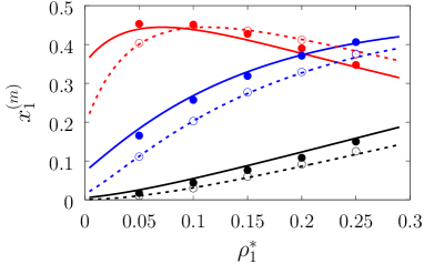
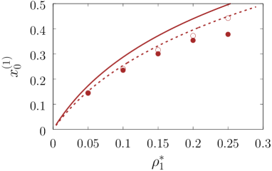
Figure 4: Fraction of $m$ times bonded fluid (top panel) and matrix (bottom panel) particles $x_{i}^{(m)}$ as a function of the fluid density $\rho_{1}^{*}$ for the model $L3M1$ at different values of the $\eta_{0}$, i.e. $\eta_{0}=0.1$ (dashed lines and open circles) and $\eta_{0}=0.2$ (solid lines and filled circles). Here $m=1$ (red and brown curves and symbols), $m=2$ (blue lines and symbols) and $m=3$ (black lines and symbols). Theoretical results are represented by the lines and computer simulation results by the symbols.

The width $\omega_{ij}$ of the square-well potential is assumed to be $0.119\sigma_{1}$ for all patch-patch interactions ensuring formation of only one bond per patch. The depth $\epsilon_{ij}$ is also taken to be the same for all the square-well potentials, assuming that the matrix particles are functionalized with same groups as the fluid particles, or at least they lead to the association between fluid and matrix particles with the energy close to that observed between fluid particles. In Fig. 2 some snapshots with examples of the simulated systems are shown.

Each simulation process was conducted in two stages: equilibration and production runs, and both runs took $10^{6}$ simulation steps, where the simulation step consisted of $N$ trial translational and rotational moves of fluid particles. It appeared to be sufficient for producing reliable data, which were obtained for two values of the packing fractions of matrix particles $\eta_{0}=\pi\rho_{0}\sigma_{0}^{3}/6$, i.e. $\eta_{0}=0.1$ and $0.2$ and different number densities of fluid particles ranging from $\rho_{1}^{*}=\sigma_{1}^{3}N_{1}/V=0.05$ up to $\rho_{1}^{*}=0.25$, where $N_{1}$ is a number of fluid particles and $V=L^{3}$ is a volume of the simulation box. The packing fraction of the matrix is an inverse characteristic to the porosity $\phi_{0}=1-\eta_{0}$, which is the basic quantity describing a porous medium, $\rho_{0}=N_{0}/V$, $N_{0}$ is a number of matrix particles and the diameter $\sigma_{0}=1.5\sigma_{1}$ was set larger than that of the fluid particles. In all simulations, a value of the temperature $T^{*}=k_{B}T/\epsilon_{11}$ was $T^{*}=0.12$, surpassing the critical temperature of the present model fluids studied in the bulk ¹⁰¹. This ensures that critical temperature of these model fluids, being confined in the matrix, is lower than $T^{*}=0.12$ ⁸¹. To accelerate the simulations the linked-cells algorithm was used with a cell size of $4.0\sigma_{1}$ ¹⁰⁰. During the production run a number of bonds between fluid and matrix particles were collected at each $10$ simulation step and averaged along the simulation in order to calculate the fraction of $m$-times bonded fluid $x_{1}^{(m)}$ and matrix $x_{0}^{(m)}$ particles and to compare them with our theoretical predictions.

4 Results and discussion

To systematically access accuracy of the theory we have studied the properties of several versions of the model. We consider the models with different number of the attracting sites and different values of the density of the fluid and matrix particles. These versions are denoted as $L_{i}M_{j}$, where $i$ and $j$ are the number of sites on the fluid and matrix particles. We also consider two values for the matrix packing fraction and one value of the temperature, i.e. $\eta_{0}=0.1,\;0.2$ and $T^{*}=k_{B}T/\epsilon_{11}=0.12$, respectively. The other parameters of the model are: $\sigma_{0}=1.5\sigma_{11}$, $\omega_{11}=\omega_{01}=0.119\sigma_{11}$ and $\epsilon_{01}=\epsilon_{11}$.

In figures 3-5 we compare theoretical and computer simulation results for the fraction of $m$ times bonded fluid $x_{1}^{(m)}$ and matrix $x_{0}^{(m)}$ particles as a function of the fluid density $\rho_{1}$. The latter quantity is calculated using the following relation ⁹⁹

$$x^{(m)}_{i}=\frac{n_{i}^{(s)}!}{m!(n_{i}^{(s)}-m)!}X_{i}^{n_{i}^{(s)}-m}(1-X_{i})^{m},$$ (12)

In figure 3 we show our results for the models with matrix particles without patches and fluid particles with 2, 3 and 4 patches, i.e. models $L2M0$, $L3P0$, and $L4P0$. Agreement between theoretical and computer simulation predictions for the models $L2M0$ and $L3M0$ at both values of the matrix packing fraction, $\eta_{0}=0.1,\;0.2$ is very good. For the model $L4M0$ and lower value of $\eta_{0}=0.1$ results of the theory are less accurate and agreement with exact computer simulation results is only semi-quantitative. However with the increase of the matrix packing fraction $\eta_{0}=0.2$ agreement between theory and computer simulation becomes almost as good as in the case of the other models. Our results for the models with patches on both fluid and matrix particles are presented in figures 4 and 5. In figure 4 we compare theoretical results against computer simulation results for the model $L3M1$. Here one can observe very good agreement between theory and simulation for $x^{(1)}_{1},x^{(2)}_{1}$ and $x^{(3)}_{1}$ for both values of the matrix packing fraction $\eta_{0}$. Theoretical predictions for the fraction of singly bonded matrix particles $x^{(1)}_{0}$ are accurate for the lower values of $\eta_{0}=0.1$. At $\eta_{0}=0.2$ theoretical results are less accurate. While computer simulations predict a slight decrease in $x^{(1)}_{0}$ upon increase of $\eta_{0}$, theoretical calculations show that it increases. As $\eta_{0}$ increases the average distance between the matrix particles decreases and the number of the obstacles with the patch blocked by the nearest neighboring obstacles increases. This effect, which is not accounted for in the framework of the present version of the TPT, causes slight decrease of $x_{0}^{(1)}$. On the other hand this effect is less pronounced for the models $L1M1$, $L1M2$ and $L1M4$ (figure 5) and the corresponding theoretical results are in a very good agreement with computer simulation results. This good agreement is observed for the fraction of $m$ times bonded fluid and matrix particles for both values of the matrix packing fraction $\eta_{0}$. Thus with the increase of the matrix packing fraction $\eta_{0}$ and number of the patches on the fluid particles $n_{1}$ the first order TPT becomes less accurate. Further improvement of the theory can be achieved using higher-order versions of the TPT.

In figures 6 and 7 we present liquid-gas phase diagram and percolation threshold lines for the model $L3M1$ with different values for the ratio between the strength of attractive fluid-fluid and fluid-matrix interaction. Percolation line separates $\rho\;vs\;T$ plane into percolating and non-percolating regions, i.e. the latter region the particles form finite size clusters and in the former these clusters form an infinite network. Our calculation of the percolation threshold lines is based on the extension of the Flory-Stockmayer theory ^{102, 101, 103, 104}. According to the earlier work ^{103, 105} percolation threshold lines for the model at hand are defined by the equality $p_{11}=1/2$, where $p_{11}$ is probability of forming the bonds between the fluid particles, i.e.

$$p_{11}=(1-X_{1})-{\rho_{0}\over 3\rho_{1}}(1-X_{0}).$$ (13)

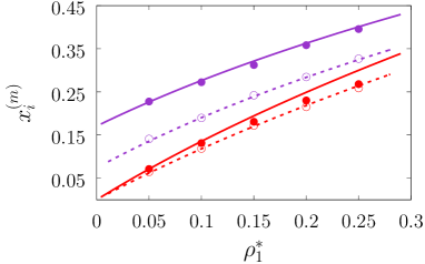
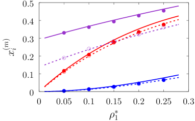
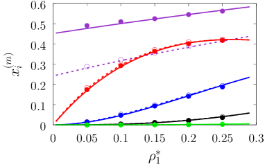
Figure 5: Fraction of $m$ times bonded fluid and matrix particles $x_{i}^{(m)}$ as a function of the fluid density $\rho_{1}^{*}$ for the model $L1M1$ (top panel), $L1M2$ (intermediate panel), $L1M4$ (bottom panel) at different values of the $\eta_{0}$, i.e. $\eta_{0}=0.1$ (dashed lines and open circles) and $\eta_{0}=0.2$ (solid lines and filled circles). Here fraction of singly bonded fluid particles ($m=1$) are shown by violet lines and symbols and for the matrix particles we have: $m=1$ (red curves and symbols), $m=2$ (blue lines and symbols), $m=3$ (black lines and symbols), $m=4$ (green line and symbols). Theoretical results are represented by the lines and computer simulation results by the symbols.

We consider the following values for the hard-sphere size of the matrix obstacles, i.e. $\sigma_{01}=1.388\sigma_{11}$ and for the width and depth of the potential well (2): $\omega_{01}=0.1\sigma_{1}$ and $\epsilon_{01}=0,\;0.77\epsilon_{11},\;0.825\epsilon_{11}$. All the rest of the potential model parameters are the same as those used before. This choice of parameters allows us to study effects due to the competition between formation of the bonds connecting fluid particles and fluid particles and matrix particles. While formation of the 3-dimensional network of bonds connecting the fluid particles causes gas-liquid phase separation, bonding of the fluid and matrix particles suppress it. For the model with $\epsilon_{01}=0$ the phase diagram is of the usual form, i.e. the difference between the coexisting densities of the gas and liquid phases increases on decreasing temperature (figure 6). Here, since the density of the gas phase $\rho_{1,gas}$ is lower than the density of the liquid phase $\rho_{1,liq}$ the fraction of the free (or three time bonded) particles in the gas phase $x_{1,gas}^{(0)}$ ($x_{1,gas}^{(3)}$) is larger (lower) than corresponding fractions in the liquid phase (figure 7, top panel). As one would expect for the fractions of free matrix particles we have $x_{0,gas}^{(0)}=x_{0,liq}^{(0)}=1$, where $x_{0,gas}^{(0)}$ and $x_{0,liq}^{(0)}$ denote fractions of free (nonbonded) particles of the matrix, which confine fluid particles either in the gas phase or in the liquid phase, respectively. Increase of $\epsilon_{01}$ causes changes of the phase diagram topology. For the model with $\epsilon_{01}=0.77\epsilon_{11}$ the phase diagram exhibits re-entrant phase behavior, i.e. decrease of the temperature in the range of approximately $0.065\geq T^{*}\geq 0.046$ results in the reduction of the difference in coexisting gas and liquid densities (figure 6). This effect is caused by the increased bonding of the fluid particles and matrix obstacles, which destroys the three-dimensional network formed by the fluid particles and suppresses the phase separation. In this range of temperatures the fraction of free obstacles $x_{0}^{(0)}$ in both phases rapidly decreases (figure 7, intermediate panel).

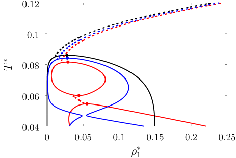
Figure 6: Liquid-gas phase diagram (solid lines) and percolation thresholds (dashed lines) for the model $L1M3$ with $\omega_{01}=0.1\sigma_{1}$ and $\epsilon_{01}=0$ (black lines), $\epsilon_{01}=0.77\epsilon_{11}$ (blue lines) and $\epsilon_{01}=0.825\epsilon_{11}$ (red lines). Here symbols denote position of the corresponding critical points.

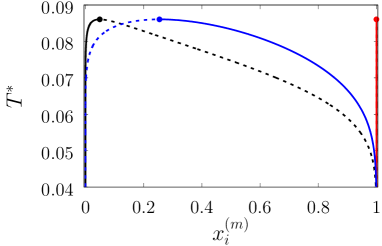
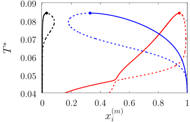
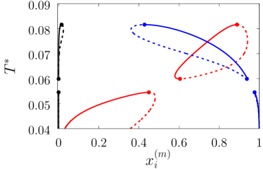
Figure 7: Fraction of $m$ time bonded fluid and matrix particles $x^{(m)}_{i}$ along coexisting lines for the model $L1M3$ with $\omega_{01}=0.1\sigma_{1}$ and $\epsilon_{01}=0$ (top panel), $\epsilon_{01}=0.77\epsilon_{11}$ (intermediate panel) and $\epsilon_{11}=0.825\epsilon_{11}$ (bottom panel). $x_{1}^{(0)}$ (black lines), $x_{1}^{(3)}$ (blue lines) and $x_{0}^{(0)}$ (red lines). Here dashed and solid lines represent gas and liquid branches of the phase diagrams, respectively.

At the same time, while the fractions of free and three times bonded fluid particles in the liquid phase do not change much, in the gas phase they are approaching the liquid phase values (figure 7, intermediate panel). This behavior reflect the process of breaking the bonds between the fluid particles and their substitution by the bonds formed between the fluid particles and obstacles of the matrix. Upon reaching sufficient bonding degree of the matrix obstacles this process slows down and with further decrease of the temperature ($T^{*}<0.046$), the three-dimensional network formed by the fluid particles becomes stronger. As a result the difference between coexisting gas and liquid densities increases with the temperature decrease (figure 6). Similar behavior can be observed for the model with $\epsilon_{01}=1.835\epsilon_{11}$. However stronger fluid-matrix attraction completely suppresses the phase separation in the range of the temperatures $0.060\leq T^{*}\leq 0.0545$. As a result we have the phase diagram with two separate regions of the liquid-gas phase coexistence: the region at higher temperatures has the upper and lower critical points (figures 6 and 7) and the region at lower temperatures has the usual liquid-gas type of the critical point. These critical points and the liquid branches of the phase diagrams are located inside percolating region (figure 6). The corresponding percolation line consists of two branches, i.e. high-temperature branch and low-temperature branch. The former branch is located at higher temperatures with cluster fluid phase above and percolating fluid phase below percolation threshold line. The latter branch is located at lower temperatures and connects high-temperature and low-temperature regions of the phase diagram. Here the percolating fluid phase occurs above and cluster fluid phase below percolation threshold line. For the models with $\epsilon_{01}=0\;\rm{and}\;0.77\epsilon_{11}$ percolation threshold lines are of the usual shape and almost completely coincide with the high-temperature percolation threshold line for the model with $\epsilon_{01}=0.825\epsilon_{11}$. Finally, we note that recently the phase behavior of the patchy colloids adsorbed in the attractive random porous medium was studied ^{88, 89}. In these studies the medium was represented as a matrix of hard-sphere obstacles with attractive Yukawa interaction between the centers of the fluid and matrix particles. Similar to the present study, confinement causes the system to undergo re-entrant liquid-gas phase separation. However competition between Yukawa interaction and bonding do not cause the phase diagram to be separated into two (or more) regions. Taking into account the good agreement between the theoretical and computer simulation predictions for the fractions $X_{0}$ and $X_{1}$ and the fact that these are the only quantities, that enter into expressions for Helmholtz free energy $\Delta A_{as}$ (4) and probability of forming the bonds $p_{11}$ (13) there are good reasons to believe that our theory is accurate enough to at least qualitatively predict the peculiarities of the phase behavior discussed above. In a subsequent paper we are planning to systematically investigate the phase behavior and percolation properties of the model using an extension of the aggregation-volume-bias MC method ^{106, 107} and the theory developed herein.

5 Conclusions

In this work we propose a simple model of functionalized disordered porous media represented by the matrix of hard-sphere fluid particles quenched at equilibrium and decorated by the certain number of the off-center square-well sites. The model is used to study effects of confinement on the clusterization, percolation and phase behavior of the fluid of patchy particles adsorbed in such porous media. The study is carried out combining Wertheim’s TPT for associating fluids, SPT for the porous media and Flory-Stockmayer theory of polymerization. A set of computer simulation data has been generated and used to assess the accuracy of the theory. Very good agreement between theoretical and computer simulation predictions is observed for the fractions of $m$-times bonded fluid and matrix particles almost in all cases studied. Slightly less accurate are results for the fraction of $m$-times bonded matrix particles for the model with fluid particles bearing more than one patch. Further improvement of the theory can be achieved using higher-order versions of the TPT.

The liquid-gas phase diagram and percolation threshold line for the model with three-patch fluid particles and one-patch matrix particles are calculated and analyzed. It is demonstrated that confinement can substantially change the shape of the phase diagram. Bonding between the fluid particles causes formation of a network and bonding of the fluid particles to the obstacles suppresses this process. Competition between these two effects define the shape of the phase diagram and gives rise to a re-entrant phase behavior with three critical points and two separate regions of the liquid-gas phase coexistence.

Appendix

Expressions for Helmholtz free energy, chemical potential and pressure of the hard-sphere fluid confined in the hard-sphere matrix

The reference system is represented by the hard-sphere fluid confined in the hard-sphere matrix. According to SPT ^{79, 54, 80, 81} we have the following expressions for Helmholtz free energy $A_{hs}$ and for the contact values of the radial distribution functions $g^{hs)}_{10}(r)$ and $g^{(hs)}_{11}(r)$ for hard-sphere fluid adsorbed in the hard-sphere matrix, i.e.

$$\beta\Delta A_{hs}\over N_{hs}=\beta\Delta\mu_{hs}-{\beta\Delta P_{hs}\over\rho_{hs}}$$ (A1)

and

$$g_{1j}^{(hs)}={1\over\phi_{0}-\eta_{1}}+{3\over 1+\tau_{1j}}{(\eta_{1}+\eta_{0}\tau_{10})\over(\phi_{0}-\eta_{1})^{2}}$$ (A2)

where $N_{hs}$ is the number of hard-sphere particles of the fluid,

$${\beta\Delta P_{hs}\over\rho_{hs}}={1\over 1-\eta_{1}/\phi_{0}}{\phi_{0}\over\phi}+\left({\phi_{0}\over\phi}-1\right){\phi_{0}\over\eta_{1}}\ln\left(1-{\eta_{1}\over\phi_{0}}\right)$$

$$+{a\over 2}{\eta_{1}/\phi_{0}\over(1-\eta_{1}/\phi_{0})^{2}}+{2b\over 3}{(\eta_{1}/\phi_{0})^{2}\over(1-\eta_{1}/\phi_{0})^{3}}-1,$$ (A3)

$$\beta\Delta\mu_{hs}=\beta\mu^{(ex)}_{1}-\ln\left(1-{\eta_{1}\over\phi_{0}}\right)+{\eta_{1}(\phi_{0}-\phi)\over\phi_{0}\phi(1-\eta_{1}/\phi_{0})}+\left(1+a\right){\eta_{1}/\phi_{0}\over(1-\eta_{1}/\phi_{0})}$$

$$+{(a+2b)\over 2}{(\eta_{1}/\phi_{0})^{2}\over(1-\eta_{1}/\phi_{0})^{2}}+{2b\over 3}{(\eta_{1}/\phi_{0})^{3}\over(1-\eta_{1}/\phi_{0})^{3}},$$ (A4)

$\eta_{0}=\pi\rho_{0}\sigma_{0}^{3}/6$, $\phi_{0}=1-\eta_{0}$, $\eta_{1}=\pi\rho_{1}\sigma_{1}^{3}/6$ and $\phi=\exp{(-\beta\mu^{(ex)}_{1})}$.

Here

$$a=6+{3\eta_{0}\tau_{10}\left(\tau_{10}+4\right)\over 1-\eta_{0}}+{9\eta_{0}^{2}\tau_{10}^{2}\over(1-\eta_{0})^{2}},\;\;\;\;\;\;\;\;\;\;\;\;b={9\over 2}\left(1+{\tau_{10}\eta_{0}\over 1-\eta_{0}}\right)^{2},$$ (A5)

$$\beta\mu_{1}^{(ex)}=-\ln{(1-\eta_{0})}+{9\eta_{0}^{2}\over 2(1-\eta_{0})^{2}}-\eta_{0}Z_{0}+\left[3\eta_{0}Z_{0}-{3\eta_{0}(2+\eta_{0})\over(1-\eta_{0})^{2}}\right](1+\tau_{10})$$

$$-\left[3\eta_{0}Z_{0}-{3\eta_{0}(2+\eta_{0})\over 2(1-\eta_{0})^{2}}\right](1+\tau_{10})^{2}+\eta_{0}Z_{0}(1+\tau_{10})^{3},$$ (A6)

$Z_{0}=(1+\eta_{0}+\eta_{0}^{2})/(1-\eta_{0})^{3}$, $\tau_{1j}=\sigma_{1}/\sigma_{j}$ and $j=0,1$.

References

- Corma 1997 Corma, A.. From microporous to mesoporous molecular sieve materials and their use in catalysis. Chem Rev 1997;97(6):2373--2420. URL: https://doi.org/10.1021%2Fcr960406n. doi:10.1021/cr960406n.
- Vinu et al. 2006 Vinu, A., Mori, T., Ariga, K.. New families of mesoporous materials. Sci Technol Adv Mater 2006;7(8):753--771. URL: https://doi.org/10.1016%2Fj.stam.2006.10.007. doi:10.1016/j.stam.2006.10.007.
- Slowing et al. 2007 Slowing, I., Trewyn, B., Giri, S., Lin, V.Y.. Mesoporous silica nanoparticles for drug delivery and biosensing applications. Adv Funct Mater 2007;17(8):1225--1236. URL: https://doi.org/10.1002%2Fadfm.200601191. doi:10.1002/adfm.200601191.
- Ertl et al. 2008 Ertl, G., Knözinger, H., Schüth, F., Weitkamp, J., eds. Handbook of Heterogeneous Catalysis. Wiley; 2008. URL: https://doi.org/10.1002%2F9783527610044. doi:10.1002/9783527610044.
- Adiga et al. 2009 Adiga, S.P., Jin, C., Curtiss, L.A., Monteiro-Riviere, N.A., Narayan, R.J.. Nanoporous membranes for medical and biological applications. Wiley Interdiscip Rev Nanomed Nanobiotechnol 2009;1(5):568--581. URL: https://doi.org/10.1002%2Fwnan.50. doi:10.1002/wnan.50.
- Corma et al. 2010 Corma, A., García, H., i Xamena, F.X.L.. Engineering metal organic frameworks for heterogeneous catalysis. Chem Rev 2010;110(8):4606--4655. URL: https://doi.org/10.1021%2Fcr9003924. doi:10.1021/cr9003924.
- Stroeve and Ileri 2011 Stroeve, P., Ileri, N.. Biotechnical and other applications of nanoporous membranes. Trends Biotechnol 2011;29(6):259--266. URL: https://doi.org/10.1016%2Fj.tibtech.2011.02.002. doi:10.1016/j.tibtech.2011.02.002.
- Misaelides 2011 Misaelides, P.. Application of natural zeolites in environmental remediation: A short review. Microporous Mesoporous Mater 2011;144(1-3):15--18.
- Dawson et al. 2012 Dawson, R., Cooper, A.I., Adams, D.J.. Nanoporous organic polymer networks. Prog Polym Sci 2012;37(4):530--563. URL: https://doi.org/10.1016%2Fj.progpolymsci.2011.09.002. doi:10.1016/j.progpolymsci.2011.09.002.
- Rouquerol et al. 2013 Rouquerol, J., Rouquerol, F., Llewellyn, P., Maurin, G., Sing, K.S.. Adsorption by powders and porous solids: principles, methodology and applications. Academic press; 2013.
- Liu et al. 2014 Liu, J., Chen, L., Cui, H., Zhang, J., Zhang, L., Su, C.Y.. Applications of metal–organic frameworks in heterogeneous supramolecular catalysis. Chem Soc Rev 2014;43(16):6011--6061. URL: https://doi.org/10.1039%2Fc4cs00094c. doi:10.1039/c4cs00094c.
- Zhang and Lin 2014 Zhang, T., Lin, W.. Metal–organic frameworks for artificial photosynthesis and photocatalysis. Chem Soc Rev 2014;43(16):5982--5993. URL: https://doi.org/10.1039%2Fc4cs00103f. doi:10.1039/c4cs00103f.
- Canham 2014 Canham, L.. Handbook of porous silicon. Springer International Publishing Berlin, Germany; 2014.
- Pal and Bhaumik 2015 Pal, N., Bhaumik, A.. Mesoporous materials: versatile supports in heterogeneous catalysis for liquid phase catalytic transformations. RSC Adv 2015;5(31):24363--24391. URL: https://doi.org/10.1039%2Fc4ra13077d. doi:10.1039/c4ra13077d.
- Li et al. 2016 Li, Y., Xu, H., Ouyang, S., Ye, J.. Metal–organic frameworks for photocatalysis. Phys Chem Chem Phys 2016;18(11):7563--7572. URL: https://doi.org/10.1039%2Fc5cp05885f. doi:10.1039/c5cp05885f.
- Liang et al. 2017 Liang, J., Liang, Z., Zou, R., Zhao, Y.. Heterogeneous catalysis in zeolites, mesoporous silica, and metal-organic frameworks. Adv Mater 2017;29(30):1701139. URL: https://doi.org/10.1002%2Fadma.201701139. doi:10.1002/adma.201701139.
- Kumeria et al. 2017 Kumeria, T., McInnes, S.J.P., Maher, S., Santos, A.. Porous silicon for drug delivery applications and theranostics: recent advances, critical review and perspectives. Expert Opin Drug Delivery 2017;14(12):1407--1422. URL: https://doi.org/10.1080%2F17425247.2017.1317245. doi:10.1080/17425247.2017.1317245.
- Danda and Drndić 2019 Danda, G., Drndić, M.. Two-dimensional nanopores and nanoporous membranes for ion and molecule transport. Curr Opin Biotechnol 2019;55:124--133. URL: https://doi.org/10.1016%2Fj.copbio.2018.09.002. doi:10.1016/j.copbio.2018.09.002.
- Wang and Astruc 2020 Wang, Q., Astruc, D.. State of the art and prospects in metal–organic framework (MOF)-based and MOF-derived nanocatalysis. Chem Rev 2020;120(2):1438--1511. URL: https://doi.org/10.1021%2Facs.chemrev.9b00223. doi:10.1021/acs.chemrev.9b00223.
- Miao et al. 2020 Miao, L., Song, Z., Zhu, D., Li, L., Gan, L., Liu, M.. Recent advances in carbon-based supercapacitors. Mater Adv 2020;1(5):945--966. URL: https://doi.org/10.1039%2Fd0ma00384k. doi:10.1039/d0ma00384k.
- Li and Yu 2021 Li, Y., Yu, J.. Emerging applications of zeolites in catalysis, separation and host–guest assembly. Nat Rev Mater 2021;6(12):1156--1174. URL: https://doi.org/10.1038%2Fs41578-021-00347-3. doi:10.1038/s41578-021-00347-3.
- Hosono and Uemura 2021 Hosono, N., Uemura, T.. Metal–organic frameworks as versatile media for polymer adsorption and separation. Acc Chem Res 2021;54(18):3593--3603. URL: https://doi.org/10.1021%2Facs.accounts.1c00377. doi:10.1021/acs.accounts.1c00377.
- Moretta et al. 2021 Moretta, R., Stefano, L.D., Terracciano, M., Rea, I.. Porous silicon optical devices: Recent advances in biosensing applications. Sensors 2021;21(4):1336. URL: https://doi.org/10.3390%2Fs21041336. doi:10.3390/s21041336.
- Singh et al. 2021 Singh, G., Bahadur, R., Lee, J.M., Kim, I.Y., Ruban, A.M., Davidraj, J.M., Semit, D., Karakoti, A., Muhtaseb, A.H.A., Vinu, A.. Nanoporous activated biocarbons with high surface areas from alligator weed and their excellent performance for CO2 capture at both low and high pressures. Chem Eng J 2021;406:126787. URL: https://doi.org/10.1016%2Fj.cej.2020.126787. doi:10.1016/j.cej.2020.126787.
- Saha et al. 2022 Saha, R., Mondal, B., Mukherjee, P.S.. Molecular cavity for catalysis and formation of metal nanoparticles for use in catalysis. Chem Rev 2022;122(14):12244--12307. URL: https://doi.org/10.1021%2Facs.chemrev.1c00811. doi:10.1021/acs.chemrev.1c00811.
- Hadden et al. 2022 Hadden, M., Martinez-Martin, D., Yong, K.T., Ramaswamy, Y., Singh, G.. Recent advancements in the fabrication of functional nanoporous materials and their biomedical applications. Materials 2022;15(6):2111. URL: https://doi.org/10.3390%2Fma15062111. doi:10.3390/ma15062111.
- Yue et al. 2022 Yue, B., Liu, S., Chai, Y., Wu, G., Guan, N., Li, L.. Zeolites for separation: Fundamental and application. J Energy Chem 2022;71:288--303. URL: https://doi.org/10.1016%2Fj.jechem.2022.03.035. doi:10.1016/j.jechem.2022.03.035.
- Popat et al. 2011 Popat, A., Hartono, S.B., Stahr, F., Liu, J., Qiao, S.Z., Lu, G.Q.M.. Mesoporous silica nanoparticles for bioadsorption, enzyme immobilisation, and delivery carriers. Nanoscale 2011;3(7):2801. URL: https://doi.org/10.1039%2Fc1nr10224a. doi:10.1039/c1nr10224a.
- Milton 1989 Milton, R.M.. Zeolite Synthesis; chap. 1. American Chemical Society; 1989:1--10. URL: https://doi.org/10.1021%2Fbk-1989-0398. doi:10.1021/bk-1989-0398.
- Wang and Peng 2010 Wang, S., Peng, Y.. Natural zeolites as effective adsorbents in water and wastewater treatment. Chem Eng J 2010;156(1):11--24. URL: https://doi.org/10.1016%2Fj.cej.2009.10.029. doi:10.1016/j.cej.2009.10.029.
- Xia et al. 2019 Xia, M., Chen, Z., Li, Y., Li, C., Ahmad, N.M., Cheema, W.A., Zhu, S.. Removal of hg(II) in aqueous solutions through physical and chemical adsorption principles. RSC Adv 2019;9(36):20941--20953. URL: https://doi.org/10.1039%2Fc9ra01924c. doi:10.1039/c9ra01924c.
- Gu and Yushin 2013 Gu, W., Yushin, G.. Review of nanostructured carbon materials for electrochemical capacitor applications: advantages and limitations of activated carbon, carbide-derived carbon, zeolite-templated carbon, carbon aerogels, carbon nanotubes, onion-like carbon, and graphene. Wiley Interdiscip Rev: Energy Environ 2013;3(5):424--473. URL: https://doi.org/10.1002%2Fwene.102. doi:10.1002/wene.102.
- Kistler 1931 Kistler, S.S.. Coherent expanded aerogels and jellies. Nature 1931;127(3211):741--741. URL: https://doi.org/10.1038%2F127741a0. doi:10.1038/127741a0.
- Kresge et al. 1992 Kresge, C.T., Leonowicz, M.E., Roth, W.J., Vartuli, J.C., Beck, J.S.. Ordered mesoporous molecular sieves synthesized by a liquid-crystal template mechanism. Nature 1992;359(6397):710--712. URL: https://doi.org/10.1038%2F359710a0. doi:10.1038/359710a0.
- Zhao et al. 1998 Zhao, D., Feng, J., Huo, Q., Melosh, N., Fredrickson, G.H., Chmelka, B.F., Stucky, G.D.. Triblock copolymer syntheses of mesoporous silica with periodic 50 to 300 angstrom pores. Science 1998;279(5350):548--552. URL: https://doi.org/10.1126%2Fscience.279.5350.548. doi:10.1126/science.279.5350.548.
- Li et al. 1999 Li, H., Eddaoudi, M., O'Keeffe, M., Yaghi, O.M.. Design and synthesis of an exceptionally stable and highly porous metal-organic framework. Nature 1999;402(6759):276--279. URL: https://doi.org/10.1038%2F46248. doi:10.1038/46248.
- Wen et al. 2019 Wen, M., Li, G., Liu, H., Chen, J., An, T., Yamashita, H.. Metal–organic framework-based nanomaterials for adsorption and photocatalytic degradation of gaseous pollutants: recent progress and challenges. Environ Sci: Nano 2019;6(4):1006--1025. URL: https://doi.org/10.1039%2Fc8en01167b. doi:10.1039/c8en01167b.
- Easun et al. 2017 Easun, T.L., Moreau, F., Yan, Y., Yang, S., Schrøder, M.. Structural and dynamic studies of substrate binding in porous metal–organic frameworks. Chem Soc Rev 2017;46(1):239--274. URL: https://doi.org/10.1039%2Fc6cs00603e. doi:10.1039/c6cs00603e.
- Li et al. 2009 Li, J.R., Kuppler, R.J., Zhou, H.C.. Selective gas adsorption and separation in metal–organic frameworks. Chem Soc Rev 2009;38(5):1477. URL: https://doi.org/10.1039%2Fb802426j. doi:10.1039/b802426j.
- Zhang et al. 2020 Zhang, X., Chen, Z., Liu, X., Hanna, S.L., Wang, X., Taheri-Ledari, R., Maleki, A., Li, P., Farha, O.K.. A historical overview of the activation and porosity of metal–organic frameworks. Chem Soc Rev 2020;49(20):7406--7427. URL: https://doi.org/10.1039%2Fd0cs00997k. doi:10.1039/d0cs00997k.
- Mizoshita et al. 2011 Mizoshita, N., Tani, T., Inagaki, S.. Syntheses, properties and applications of periodic mesoporous organosilicas prepared from bridged organosilane precursors. Chem Soc Rev 2011;40(2):789--800. URL: https://doi.org/10.1039%2Fc0cs00010h. doi:10.1039/c0cs00010h.
- Modak et al. 2010 Modak, A., Mondal, J., Aswal, V.K., Bhaumik, A.. A new periodic mesoporous organosilica containing diimine-phloroglucinol, pd(ii)-grafting and its excellent catalytic activity and trans-selectivity in c–c coupling reactions. J Mater Chem 2010;20(37):8099. URL: https://doi.org/10.1039%2Fc0jm01180k. doi:10.1039/c0jm01180k.
- McKeown et al. 2006 McKeown, N.B., Gahnem, B., Msayib, K.J., Budd, P.M., Tattershall, C.E., Mahmood, K., Tan, S., Book, D., Langmi, H.W., Walton, A.. Towards polymer-based hydrogen storage materials: Engineering ultramicroporous cavities within polymers of intrinsic microporosity. Angew Chem Int Ed 2006;45(11):1804--1807. URL: https://doi.org/10.1002%2Fanie.200504241. doi:10.1002/anie.200504241.
- Wu et al. 2012 Wu, D., Xu, F., Sun, B., Fu, R., He, H., Matyjaszewski, K.. Design and preparation of porous polymers. Chem Rev 2012;112(7):3959--4015. URL: https://doi.org/10.1021%2Fcr200440z. doi:10.1021/cr200440z.
- Chandra and Bhaumik 2009 Chandra, D., Bhaumik, A.. A new functionalized mesoporous polymer with high efficiency for the removal of pollutant anions. J Mater Chem 2009;19(13):1901. URL: https://doi.org/10.1039%2Fb818248e. doi:10.1039/b818248e.
- Ou et al. 2018 Ou, H., Zhang, W., Yang, X., Cheng, Q., Liao, G., Xia, H., Wang, D.. One-pot synthesis of g-c3n4-doped amine-rich porous organic polymer for chlorophenol removal. Environ Sci: Nano 2018;5(1):169--182. URL: https://doi.org/10.1039%2Fc7en00787f. doi:10.1039/c7en00787f.
- Xu et al. 2013 Xu, Y., Jin, S., Xu, H., Nagai, A., Jiang, D.. Conjugated microporous polymers: design, synthesis and application. Chem Soc Rev 2013;42(20):8012. URL: https://doi.org/10.1039%2Fc3cs60160a. doi:10.1039/c3cs60160a.
- Das et al. 2017 Das, S., Heasman, P., Ben, T., Qiu, S.. Porous organic materials: Strategic design and structure–function correlation. Chem Rev 2017;117(3):1515--1563. URL: https://doi.org/10.1021%2Facs.chemrev.6b00439. doi:10.1021/acs.chemrev.6b00439.
- Ding and Wang 2013 Ding, S.Y., Wang, W.. Covalent organic frameworks (COFs): from design to applications. Chem Soc Rev 2013;42(2):548--568. URL: https://doi.org/10.1039%2Fc2cs35072f. doi:10.1039/c2cs35072f.
- Geng et al. 2020 Geng, K., He, T., Liu, R., Dalapati, S., Tan, K.T., Li, Z., Tao, S., Gong, Y., Jiang, Q., Jiang, D.. Covalent organic frameworks: Design, synthesis, and functions. Chem Rev 2020;120(16):8814--8933. URL: https://doi.org/10.1021%2Facs.chemrev.9b00550. doi:10.1021/acs.chemrev.9b00550.
- Yadav et al. 2020 Yadav, R., Baskaran, T., Kaiprathu, A., Ahmed, M., Bhosale, S.V., Joseph, S., Al-Muhtaseb, A.H., Singh, G., Sakthivel, A., Vinu, A.. Recent advances in the preparation and applications of organo-functionalized porous materials. Chem Asian J 2020;15(17):2588--2621. URL: https://doi.org/10.1002%2Fasia.202000651. doi:10.1002/asia.202000651.
- Rosinberg 1999 Rosinberg, M.L.. New Approaches to Problems in Liquid State Theory. NATO Science Series; vol. 529. Dordrecht: Springer; 1999:245--278. URL: https://doi.org/10.1007%2F978-94-011-4564-0_13. doi:10.1007/978-94-011-4564-0_13.
- Sarkisov and Tassel 2008 Sarkisov, L., Tassel, P.R.V.. Theories of molecular fluids confined in disordered porous materials. J Phys: Condens Matter 2008;20(33):333101. URL: https://doi.org/10.1088%2F0953-8984%2F20%2F33%2F333101. doi:10.1088/0953-8984/20/33/333101.
- Holovko et al. 2013 Holovko, M., Patsahan, T., Dong, W.. Fluids in random porous media: Scaled particle theory. Pure Appl Chem 2013;85(1):115--133. URL: https://doi.org/10.1351%2Fpac-con-12-05-06. doi:10.1351/pac-con-12-05-06.
- Holovko et al. 2015a Holovko, M., Shmotolokha, V., Patsahan, T.. Physics of Liquid Matter: Modern Problems. Springer Proceedings in Physics; vol. 171 of Springer Proceedings in Physics; chap. 1. Cham: Springer; 2015a:3--30. URL: https://doi.org/10.1007/978-3-319-20875-6_1. doi:10.1007/978-3-319-20875-6_1.
- Dong and Chen 2018 Dong, W., Chen, X.. Scaled particle theory for bulk and confined fluids: A review. Sci China Phys, Mech Astron 2018;61:70501. URL: https://doi.org/10.1007%2Fs11433-017-9165-y. doi:10.1007/s11433-017-9165-y.
- Pizio 2019 Pizio, O.. Computational Methods in Surface and Colloid Science; chap. 6. United States: CRC Press; 2019:293--345. URL: https://doi.org/10.1201%2F9780429115813-6. doi:10.1201/9780429115813-6.
- Madden and Glandt 1988 Madden, W.G., Glandt, E.D.. Distribution functions for fluids in random media. J Stat Phys 1988;51(3-4):537--558. URL: https://doi.org/10.1007%2Fbf01028471. doi:10.1007/bf01028471.
- Madden 1992 Madden, W.G.. Fluid distributions in random media: Arbitrary matrices. J Chem Phys 1992;96(7):5422--5432. URL: https://doi.org/10.1063%2F1.462726. doi:10.1063/1.462726.
- Given and Stell 1992 Given, J.A., Stell, G.. Comment on: Fluid distributions in two-phase random media: Arbitrary matrices. J Chem Phys 1992;97(6):4573--4574. URL: https://doi.org/10.1063%2F1.463883. doi:10.1063/1.463883.
- Kovalenko and Hirata 2001 Kovalenko, A., Hirata, F.. A replica reference interaction site model theory for a polar molecular liquid sorbed in a disordered microporous material with polar chemical groups. J Chem Phys 2001;115(18):8620--8633. URL: https://doi.org/10.1063%2F1.1409954. doi:10.1063/1.1409954.
- Chandler 1991 Chandler, D.. RISM equations for fluids in quenched amorphous materials. J Phys: Condens Matter 1991;3(42):F1--F8. URL: https://doi.org/10.1088%2F0953-8984%2F3%2F42%2F001. doi:10.1088/0953-8984/3/42/001.
- Thompson and Glandt 1993 Thompson, A.P., Glandt, E.D.. Adsorption of polymeric fluids in microporous materials. i. ideal freely jointed chains. J Chem Phys 1993;99(10):8325--8329. URL: https://doi.org/10.1063%2F1.465605. doi:10.1063/1.465605.
- Trokhymchuk et al. 1997 Trokhymchuk, A., Pizio, O., Holovko, M., Sokolowski, S.. Associative replica ornstein–zernike equations and the structure of chemically reacting fluids in porous media. J Chem Phys 1997;106(1):200--209. URL: https://doi.org/10.1063%2F1.473042. doi:10.1063/1.473042.
- Orozco et al. 1997 Orozco, G.A., Pizio, O., Sokolowski, S., Trokhymchuk, A.. Replica ornstein—zernike theory for chemically associating fluids with directional forces in disordered porous media: Smith—nezbeda model in a hard sphere matrix. Mol Phys 1997;91(4):625--634. URL: https://doi.org/10.1080%2F00268979709482752. doi:10.1080/00268979709482752.
- Pizio et al. 1998 Pizio, O., Duda, Y., Trokhymchuk, A., Sokolowski, S.. Associative replica ornstein-zernike equations and the structure of chemically associating fluids in disordered porous media. J Mol Liq 1998;76(3):183--194. URL: https://doi.org/10.1016%2Fs0167-7322%2898%2900062-2. doi:10.1016/s0167-7322(98)00062-2.
- Padilla et al. 1998 Padilla, P., Pizio, O., Trokhymchuk, A., Vega, C.. Adsorption of dimerizing and dimer fluids in disordered porous media. J Phys Chem B 1998;102(16):3012--3017. URL: https://doi.org/10.1021%2Fjp973455s. doi:10.1021/jp973455s.
- Malo et al. 1999 Malo, B.M., Pizio, O., Trokhymchuk, A., Duda, Y.. Adsorption of a hard sphere fluid in disordered microporous quenched matrix of short chain molecules: Integral equations and grand canonical monte carlo simulations. J Colloid Interface Sci 1999;211(2):387--394. URL: https://doi.org/10.1006%2Fjcis.1998.6025. doi:10.1006/jcis.1998.6025.
- Urbic et al. 2004 Urbic, T., Vlachy, V., Pizio, O., Dill, K.. Water-like fluid in the presence of lennard–jones obstacles: predictions of an associative replica ornstein–zernike theory. J Mol Liq 2004;112(1-2):71--80. URL: https://doi.org/10.1016%2Fj.molliq.2003.12.001. doi:10.1016/j.molliq.2003.12.001.
- Hribar et al. 1997 Hribar, B., Pizio, O., Trokhymchuk, A., Vlachy, V.. Screening of ion–ion correlations in electrolyte solutions adsorbed in electroneutral disordered matrices of charged particles: Application of replica ornstein–zernike equations. J Chem Phys 1997;107(16):6335--6341. URL: https://doi.org/10.1063%2F1.474294. doi:10.1063/1.474294.
- Hribar et al. 1998 Hribar, B., Pizio, O., Trokhymchuk, A., Vlachy, V.. Ion–ion correlations in electrolyte solutions adsorbed in disordered electroneutral charged matrices from replica ornstein–zernike equations. J Chem Phys 1998;109(6):2480--2489. URL: https://doi.org/10.1063%2F1.476819. doi:10.1063/1.476819.
- Hribar et al. 1999 Hribar, B., Vlachy, V., Trokhymchuk, A., Pizio, O.. Structure and thermodynamics of asymmetric electrolytes adsorbed in disordered electroneutral charged matrices from replica ornstein-zernike equations. J Phys Chem B 1999;103(25):5361--5369. URL: https://doi.org/10.1021%2Fjp990253i. doi:10.1021/jp990253i.
- Vlachy et al. 2004 Vlachy, V., Dominguez, H., Pizio, O.. Temperature effects in adsorption of a primitive model electrolyte in disordered quenched media: Predictions of the replica OZ/HNC approximation. J Phys Chem B 2004;108(3):1046--1055. URL: https://doi.org/10.1021%2Fjp035166b. doi:10.1021/jp035166b.
- Hribar-Lee et al. 2011 Hribar-Lee, B., Lukšič, M., Vlachy, V.. Partly-quenched systems containing charges. structure and dynamics of ions in nanoporous materials. Annu Rep R Soc Chem Sect C Phys Chem 2011;107:14. URL: https://doi.org/10.1039%2Fc1pc90001c. doi:10.1039/c1pc90001c.
- Pizio and Sokolowski 1997 Pizio, O., Sokolowski, S.. Adsorption of fluids in confined disordered media from inhomogeneous replica ornstein-zernike equations. Phys Rev E 1997;56(1):R63--R66. URL: https://doi.org/10.1103%2Fphysreve.56.r63. doi:10.1103/physreve.56.r63.
- Kovalenko et al. 1998 Kovalenko, A., Sokołowski, S., Henderson, D., Pizio, O.. Adsorption of a hard sphere fluid in a slitlike pore filled with a disordered matrix by the inhomogeneous replica ornstein-zernike equations. Phys Rev E 1998;57(2):1824--1831. URL: https://doi.org/10.1103%2Fphysreve.57.1824. doi:10.1103/physreve.57.1824.
- Holovko and Dong 2009 Holovko, M., Dong, W.. A highly accurate and analytic equation of state for a hard sphere fluid in random porous media. J Phys Chem B 2009;113(18):6360--6365. URL: https://doi.org/10.1021%2Fjp809706n. doi:10.1021/jp809706n.
- Chen et al. 2010 Chen, W., Dong, W., Holovko, M., Chen, X.S.. Comment on “a highly accurate and analytic equation of state for a hard sphere fluid in random porous media”. J Phys Chem B 2010;114(2):1225--1225. URL: https://doi.org/10.1021%2Fjp9106603. doi:10.1021/jp9106603.
- Patsahan et al. 2011 Patsahan, T., Holovko, M., Dong, W.. Fluids in porous media. III. scaled particle theory. J Chem Phys 2011;134(7):074503. URL: https://doi.org/10.1063%2F1.3532546. doi:10.1063/1.3532546.
- Holovko et al. 2017a Holovko, , Patsahan, , Dong, . On the improvement of SPT2 approach in the theory of a hard sphere fluid in disordered porous media. Condens Matter Phys 2017a;20(3):33602. URL: https://doi.org/10.5488%2Fcmp.20.33602. doi:10.5488/cmp.20.33602.
- Kalyuzhnyi et al. 2014 Kalyuzhnyi, Y.V., Holovko, M., Patsahan, T., Cummings, P.T.. Phase behavior and percolation properties of the patchy colloidal fluids in the random porous media. J Phys Chem Lett 2014;5(24):4260--4264. URL: https://doi.org/10.1021%2Fjz502135f. doi:10.1021/jz502135f.
- Reiss et al. 1959 Reiss, H., Frisch, H.L., Lebowitz, J.L.. Statistical mechanics of rigid spheres. J Chem Phys 1959;31(2):369--380. URL: https://doi.org/10.1063%2F1.1730361. doi:10.1063/1.1730361.
- Holovko et al. 2015b Holovko, , Patsahan, , Shmotolokha, . What is liquid in random porous media: the barker-henderson perturbation theory. Condens Matter Phys 2015b;18(1):13607. URL: https://doi.org/10.5488%2Fcmp.18.13607. doi:10.5488/cmp.18.13607.
- Nelson et al. 2020 Nelson, A., Kalyuzhnyi, Y., Patsahan, T., McCabe, C.. Liquid-vapor phase equilibrium of a simple liquid confined in a random porous media: Second-order barker-henderson perturbation theory and scaled particle theory. J Mol Liq 2020;300:112348. URL: https://doi.org/10.1016%2Fj.molliq.2019.112348. doi:10.1016/j.molliq.2019.112348.
- Hvozd and Kalyuzhnyi 2017 Hvozd, T.V., Kalyuzhnyi, Y.V.. Two- and three-phase equilibria of polydisperse yukawa hard-sphere fluids confined in random porous media: high temperature approximation and scaled particle theory. Soft Matter 2017;13(7):1405--1412. URL: https://doi.org/10.1039%2Fc6sm02613c. doi:10.1039/c6sm02613c.
- Hvozd et al. 2018 Hvozd, T.V., Kalyuzhnyi, Y.V., Cummings, P.T.. Phase equilibria of polydisperse square-well chain fluid confined in random porous media: TPT of wertheim and scaled particle theory. J Phys Chem B 2018;122(21):5458--5465. URL: https://doi.org/10.1021%2Facs.jpcb.7b11741. doi:10.1021/acs.jpcb.7b11741.
- Hvozd et al. 2020 Hvozd, T., Kalyuzhnyi, Y.V., Vlachy, V.. Aggregation, liquid–liquid phase separation, and percolation behaviour of a model antibody fluid constrained by hard-sphere obstacles. Soft Matter 2020;16(36):8432--8443. URL: https://doi.org/10.1039%2Fd0sm01014f. doi:10.1039/d0sm01014f.
- Hvozd et al. 2022a Hvozd, T.V., Kalyuzhnyi, Y.V., Vlachy, V., Cummings, P.T.. Empty liquid state and re-entrant phase behavior of the patchy colloids confined in porous media. J Chem Phys 2022a;156(16):161102. URL: https://doi.org/10.1063%2F5.0088716. doi:10.1063/5.0088716.
- Hvozd et al. 2022b Hvozd, T., Kalyuzhnyi, Y.V., Vlachy, V.. Behaviour of the model antibody fluid constrained by rigid spherical obstacles: Effects of the obstacle–antibody attraction. Soft Matter 2022b;18(47):9108--9117. URL: https://doi.org/10.1039%2Fd2sm01258h. doi:10.1039/d2sm01258h.
- Holovko and Kalyuzhnyi 1991 Holovko, M., Kalyuzhnyi, Y.V.. On the effects of association in the statistical theory of ionic systems. analytic solution of the PY-MSA version of the wertheim theory. Mol Phys 1991;73(5):1145--1157. URL: https://doi.org/10.1080%2F00268979100101831. doi:10.1080/00268979100101831.
- Krienke et al. 2000 Krienke, H., Barthel, J., Holovko, M., Protsykevich, I., Kalyushnyi, Y.. Osmotic and activity coefficients of strongly associated electrolytes over large concentration ranges from chemical model calculations. J Mol Liq 2000;87(2-3):191--216. URL: https://doi.org/10.1016%2Fs0167-7322%2800%2900121-5. doi:10.1016/s0167-7322(00)00121-5.
- Holovko et al. 2017b Holovko, M., Patsahan, T., Patsahan, O.. Effects of disordered porous media on the vapour-liquid phase equilibrium in ionic fluids: application of the association concept. J Mol Liq 2017b;228:215--223. URL: https://doi.org/10.1016%2Fj.molliq.2016.10.045. doi:10.1016/j.molliq.2016.10.045.
- Holovko et al. 2017c Holovko, M., Patsahan, T., Patsahan, O.. Application of the ionic association concept to the study of the phase behaviour of size-asymmetric ionic fluids in disordered porous media. J Mol Liq 2017c;235:53--59. URL: https://doi.org/10.1016%2Fj.molliq.2016.11.030. doi:10.1016/j.molliq.2016.11.030.
- Holovko et al. 2016 Holovko, M.F., Patsahan, O., Patsahan, T.. Vapour-liquid phase diagram for an ionic fluid in a random porous medium. J Phys: Condens Matter 2016;28(41):414003. URL: https://doi.org/10.1088%2F0953-8984%2F28%2F41%2F414003. doi:10.1088/0953-8984/28/41/414003.
- Patsahan et al. 2018a Patsahan, O.V., Patsahan, T.M., Holovko, M.F.. Vapor-liquid phase behavior of a size-asymmetric model of ionic fluids confined in a disordered matrix: The collective-variables-based approach. Phys Rev E 2018a;97(2):022109. URL: https://doi.org/10.1103%2Fphysreve.97.022109. doi:10.1103/physreve.97.022109.
- Patsahan et al. 2018b Patsahan, O., Patsahan, T., Holovko, M.. Vapour-liquid critical parameters of a 2:1 primitive model of ionic fluids confined in disordered porous media. J Mol Liq 2018b;270:97--105. URL: https://doi.org/10.1016%2Fj.molliq.2017.12.033. doi:10.1016/j.molliq.2017.12.033.
- Wertheim 1986a Wertheim, M.S.. Fluids with highly directional attractive forces. III. multiple attraction sites. J Stat Phys 1986a;42(3-4):459--476. URL: https://doi.org/10.1007%2Fbf01127721. doi:10.1007/bf01127721.
- Wertheim 1986b Wertheim, M.S.. Fluids with highly directional attractive forces. IV. equilibrium polymerization. J Stat Phys 1986b;42(3-4):477--492. URL: https://doi.org/10.1007%2Fbf01127722. doi:10.1007/bf01127722.
- Wertheim 1987 Wertheim, M.S.. Thermodynamic perturbation theory of polymerization. J Chem Phys 1987;87(12):7323--7331. URL: https://doi.org/10.1063%2F1.453326. doi:10.1063/1.453326.
- Allen and Tildesley 2017 Allen, M.P., Tildesley, D.J.. Computer Simulation of Liquids. Oxford University Press; 2017. URL: https://doi.org/10.1093%2Foso%2F9780198803195.001.0001. doi:10.1093/oso/9780198803195.001.0001.
- Bianchi et al. 2008 Bianchi, E., Tartaglia, P., Zaccarelli, E., Sciortino, F.. Theoretical and numerical study of the phase diagram of patchy colloids: Ordered and disordered patch arrangements. J Chem Phys 2008;128(14):144504. URL: https://doi.org/10.1063%2F1.2888997. doi:10.1063/1.2888997.
- Bianchi et al. 2007 Bianchi, E., Tartaglia, P., Nave, E.L., Sciortino, F.. Fully solvable equilibrium self-assembly process: fine-tuning the clusters size and the connectivity in patchy particle systems. J Phys Chem B 2007;111(40):11765--11769. URL: https://doi.org/10.1021%2Fjp074281%2B. doi:10.1021/jp074281+.
- de las Heras et al. 2011 de las Heras, D., Tavares, J.M., da Gama, M.M.T.. Phase diagrams of binary mixtures of patchy colloids with distinct numbers of patches: the network fluid regime. Soft Matter 2011;7(12):5615. URL: https://doi.org/10.1039%2Fc0sm01493a. doi:10.1039/c0sm01493a.
- Tavares et al. 2010 Tavares, J.M., Teixeira, P.I.C., da Gama, M.M.T., Sciortino, F.. Equilibrium self-assembly of colloids with distinct interaction sites: Thermodynamics, percolation, and cluster distribution functions. J Chem Phys 2010;132(23):234502. URL: https://doi.org/10.1063%2F1.3435346. doi:10.1063/1.3435346.
- Roldán-Vargas et al. 2013 Roldán-Vargas, S., Smallenburg, F., Kob, W., Sciortino, F.. Phase diagram of a reentrant gel of patchy particles. J Chem Phys 2013;139(24):244910. URL: https://doi.org/10.1063%2F1.4849115. doi:10.1063/1.4849115.
- Chen and Siepmann 2001 Chen, B., Siepmann, J.I.. Improving the efficiency of the aggregation- volume- bias monte carlo algorithm. J Phys Chem B 2001;105(45):11275--11282.
- Russo et al. 2011 Russo, J., Tavares, J., Teixeira, P., Da Gama, M.T., Sciortino, F.. Reentrant phase diagram of network fluids. Phys Rev Lett 2011;106(8):085703.