Fidelity and Overlap of Neural Quantum States: Error Bounds on the Monte Carlo Estimator
Abstract
Overlap between two neural quantum states can be computed through Monte Carlo sampling by evaluating the unnormalized probability amplitudes on a subset of basis configurations. Due to the presence of probability amplitude ratios in the estimator, which are possibly unbounded, convergence of this quantity is not immediately obvious. Our work provides a derivation of analytical error bounds on the overlap in the Monte Carlo calculations as a function of their fidelity and the number of samples. Special case of normalized autoregressive neural quantum states is analyzed separately.
I Introduction
Numerical simulation of many-body quantum systems on classical hardware poses a challenge due to high dimensionality of the quantum Hilbert space, growing exponentially with the system size. Exact diagonalization of many-body problems in the full Hilbert space can only be done for relatively small systems of several degrees of freedom due to memory and computational time limitations [1]. Multiple approaches to solve these problems in an approximate way have been developed to date. Among them are Quantum Monte Carlo (QMC) methods [2, 3, 4] and tensor networks (TN) [5] (for reviews see [6, 7]), which have proven successful for certain classes of low-dimensional systems with short-range entanglement. Nevertheless, TN have limitations regarding the representable space of states and a high computational cost for tensor contractions.
A possible way of solving the many-body problem is the use of Neural Quantum States (NQS), a variational neural network Ansatz for a quantum wavefunction, first introduced in [8]. The neural network maps configurations into complex probability amplitudes. Due to nonlinearities in the activation functions in the network this Ansatz can represent a larger class of states than tensor networks [9, 10] with fewer parameters (see, however, [11, 12] and in particular [13]). Parameters of the network are optimized variationally by Monte Carlo (MC) sampling of the configurations (see e.g. [14] for a pedagogical introduction). The difficulty now shifts towards costly MC sampling and navigation on the complicated optimization landscape of parameters, rather than mere expressibility of the Ansatz. Nevertheless, it has been demonstrated that NQS can be used to find ground states of 1- and 2-dimensional spin systems [15, 16], perform unitary time evolution [8, 17, 18], learn physical wavefunction from experimental data [19] or simulate open systems in contact with reservoir [20, 21, 22, 23, 24, 25].
Quantum fidelity and overlap are fundamental quantities used for measuring the distance between quantum states. They can be used e.g. to iteratively find excited states starting from the groundstate (see [26] for excited state calculation in NQS), map out phase diagrams [27, 28], or to verify how far the quantum state prepared in the lab is from the desired one [29]. In the context of approximate numerical Ansätze, such as NQS, calculation of fidelity between the approximate and exact state, although accessible only for small systems, gives a quantitative estimate on the quality of the Ansatz. It is also a useful tool in diagnosis of the unitary time evolution algorithms, as performed in [30]. Not all numerical methods of simulating many-body systems allow for a direct, efficient calculation of fidelity - see eg. algorithm introduced in [27] for 2-dimensional tensor networks.
Although the calculation of fidelities has already been successfully performed with NQS [26, 30, 31] in the standard Monte Carlo sampling fashion, and it has recently been rigorously proven it can be computed with a finite number of samples [32], in this paper we perform a detailed study of the error of such an estimate. Our calculations yield simple, analytical error bounds on both fidelity and overlap calculated with NQS via Monte Carlo sampling, which in some settings are tighter than those of Ref. [32].
This paper is organized as follows. In Section II we establish the notation and pedagogically revise how one calculates the overlap and fidelity for neural quantum states through Monte Carlo sampling. Section III is devoted to the derivation of the error bounds for both of these quantities. We separately treat the case of normalized states, eg. autoregressive neural networks (ARNN), for which sampling from only a single network is required, and the general case of unnormalized probability amplitudes. In Section IV we numerically benchmark the error bounds for a physical system. We conclude in Section V.
II Overlap and fidelity
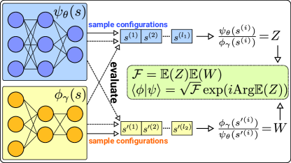
Assume that we are given two NQSs, parametrized by variational parameters , respectively, that encode approximations of two quantum states
| (1) | |||||
| (2) |
where are basis vectors of the Hilbert space with . For example, for spins-1/2, with and the number of basis elements is . We consider a general case of NQS with not necessarily equal to . Some of our results obtained for , e.g. for ARNN, are analyzed separately. We calculate the overlap
| (3) |
and fidelity . As we are dealing with NQS, we can (i) evaluate amplitudes , efficiently given configuration , (ii) generate samples of configurations coming from probability distributions and .
Although terms (3) are accessible, naive evaluation of the network on all basis elements is intractable for large systems due to the dimension of the Hilbert space growing exponentially with the system size. The normalization factors also require a summation of exponentially many terms. However, one can use a standard trick for the MC calculation of operator expectation values with NQS [8], i.e., rewrite Eq. (3) as:
| (4) |
where . Then , with configurations drawn from the probability distribution . To estimate one generates samples according to this probability distribution and constructs an empirical MC estimator
| (5) |
It is clear that .
If both states are normalized with , e.g. they are represented by an autoregressive Ansatz, one can immediately read off the overlap .
However, for unnormalized states, the preceding factor of remains unknown. This issue can be circumvented by computing
| (6) |
where and we used the same trick as in Eq. (4) but for . In the similar way as before, we can generate samples but now from from and define an estimator
| (7) |
Of course, , and fidelity reads
i.e., normalization factors cancel out, while as variables , are independent because they come from two different random processes. Using this result for the overlap, we can write
| (9) |
Note that the definition of the complex phase involves only because a ”symmetric” formula would be defined up to mod .
III Error bounds
We provide an upper bound on the number of samples (or only for the case of normalized states) required to estimate and with a fixed additive error and failure probability , see Fig. 2. The bounds are calculated using the framework first employed in [29] in the context of measuring fidelities in quantum circuits through Pauli measurements.
III.1 Normalized states
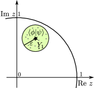
For simplicity, we first consider the case of normalized states , e.g. encoded using ARNN architectures, which generate configurations site-by-site by implementing conditional probabilities [33],
| (10) |
We use the Chebyshev’s inequality
| (11) |
which holds for any probability distribution of the random variable with finite first and second moments. It states that the probability of a single realization of achieving a value of standard deviations away from the mean is smaller than . In our case, , see Eq. (5), while
where we used and normalization of . Setting we obtain
| (13) |
where
| (14) |
That is, without any prior knowledge about the fidelity , assuming the worst-case scenario of orthogonal states with , we need at least samples from in order for the estimate to fall within a complex disk of radius around the true value with probability , see Fig. 2a. Notice that the required number of samples is independent of any properties of the state, system size and any system details such as local Hilbert space and spatial dimension. We also note that although the Central Limit Theorem guarantees that the distribution of asymptotically converges to the normal distribution on the complex plane for , the rate of convergence with depends on the details of the probability distribution of and should be computed separately for each pair of quantum states , . On the contrary, the Chebyshev’s inequality holds without the assumption of the distribution of .
The fidelity could in principle be estimated by . We were unable to provide bounds for its variance as this expression contains terms and which do not simplify as in Eq. (III.1). On the other hand, the interval in which we expect to find the estimate of follows directly from the error in overlap,
| (15) |
where was previously defined in Eq. (13). This is obtained from
where we used and is an arbitrary complex phase.
For large the fidelity error attains a maximum at . Minima of the error occur at and . At the error reaches , while for it converges to .
III.2 General case
The same technique is directly generalized to unnormalized states. First, we derive an error bound for the MC estimate of fidelity through Chebyshev’s inequality (11). Using the independence of the variables , , and Eq. (III.1), we find that
| (17) |
Full derivation is presented in the Appendix A.
Given the total number of samples , choosing equal sampling minimizes the variance. Plugging into the Chebyshev’s inequality for in Eq. (11), and using the variance formula (17), for the optimal choice of samples we obtain
| (18) |
where
| (19) |
For a large number of samples , the minimal error is obtained for and , while maximizes the error. Let us compare this result to the case of single-state sampling with the same number of samples.
Taylor expansion of as a function of around zero gives
| (20) |
This means that the leading term is the same as in Eq. (15), while a higher-order correction to the error is smaller here by a factor of . However, in practice one always uses so there are no advantages of using one or the other method, irrespective of the fidelity value .
Our error bound can be compared to that of Ref. [32], where an robust estimator based on the calculation of the median of multiple estimates of means of is considered. With a total of samples, i.e. queries of the amplitude ratios, the fidelity is estimated up to additive error with failure probability . It is straightforward to show that at the same failure probability , our error bound given by Eq. (19) is smaller, , if the condition
| (21) |
is met. In the limit of large , this is always true if since the l.h.s. is always less or equal . The inequality is also satisfied in the interesting cases when states are either close to each other, , for any , or when they are orthogonal, , for dependent on the chosen .
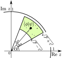
Having the fidelity interval, we can read off the error bounds for the overlap defined by Eq. (9). Since, with probability , lies in the interval , the estimator for lies in the interval with the same probability.
The error in the complex phase is due to the uncertainty of the phase in . With probability , lies in a disk of radius with a center at . The disk spreads over complex angles , and simple trigonometry gives
(If the argument under is greater than , we separately define the angle as , so that remains undefined). Thus, with probability at least , the MC estimator of lies in the region presented in Fig. 3.
IV Numerical benchmarks
IV.1 Method
We numerically validate the analytical error bounds in the following way. To simulate a generic, entangled state we consider a 1-dimensional chain of spins-1/2 and a neural network variational Ansatz with random weights (see eg. [34] for the properties of restricted Boltzmann machine NQS with Gaussian weights). In order to measure the error as a function of fidelity, we scan a range of fidelities by evolving this state in time to with the Hamiltonian of the transverse field Ising model,
| (23) |
with periodic boundary conditions , and . Time evolution up to time is performed using the time-dependent Variational Monte Carlo (tVMC) method [8, 35, 18, 36]. Our codes are available at github.com/tszoldra/jVMC_overlap. We use the TDVP [37] algorithm, implemented in jVMC 1.2.4 [38, 39] framework, with Euler integrator with timestep , regularization cutoff in the pseudoinverse of the quantum Fisher matrix and MC samples for each timestep (see [38] for details on regularization techniques). We do not care how well the variational Ansatz approximates the actual time-evolved physical wave function as we are only interested in the decrease of fidelity between the time-evolved and the initial state.
The error of the overlap estimation is measured by comparing the Monte Carlo estimate with the exact summation over all basis states as in Eq. (3) which could be done for the moderate system sizes . Cases of autoregressive and unnormalized neural networks are analyzed separately below. All results are produced using samples (in ARNN case, , in general case ) and are averaged over random initial states (random weights of the neural network) and independent MC calculations of the overlap or fidelity. Error bars denote an estimate of one standard deviation for a single sample, i.e., a deviation one may expect when computing a single estimate of the overlap or fidelity using samples in total.
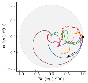
Our ARNN Ansatz is a densely connected recurrent neural network [16] with hidden size and depth , yielding real variational parameters in total, and an exponential linear unit (ELU) [40] activation function. Random initial weights come from a uniform distribution on the interval , rescaled by the square root of the average number of inputs and outputs in a given layer. Due to the autoregressive property, MC sampling of spin configurations from this network is exact, i.e. MC samples are perfectly uncorrelated. Fig. 4 shows exemplary time evolutions of an exact overlap on the complex plane.
The unnormalized Ansatz is a restricted Boltzmann machine (RBM) [8, 41] with complex parameters, hidden size of units, and no bias term. Number of complex variational weights varies between system sizes and is equal to . Random initial weights have real and complex parts uniformly distributed on the interval . We sample configurations from this NQS using Markov chain Monte Carlo Metropolis-Hastings algorithm with random spin flip as a step proposal, Monte Carlo steps for a single sweep, and sweeps for an initial ”burn-in”/thermalization.
IV.2 Results
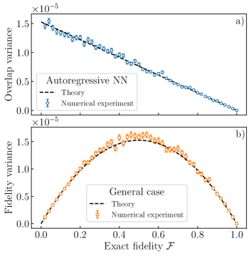
In FIG. 5 we verify the the variance formulae Eq. (III.1) for ARNN (panel a) and Eq. (17) for unnormalized NQS (panel b) for system size . In both cases, we see a very good agreement between the theoretical prediction and the numerical result within error bars. Here, unlike in all other plots, the error bars are the standard deviations from the mean value, i.e. error of the mean estimate, not a deviation expected for a single MC estimate.
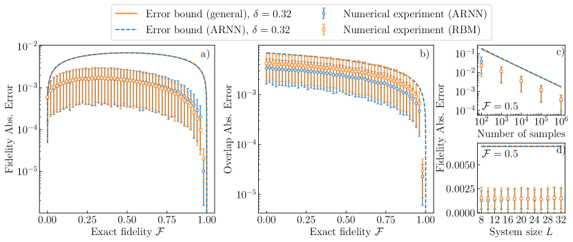
We then verify the error bounds. FIG. 6a) shows mean absolute errors of fidelity MC estimate for ARNN and RBM networks for system size . Since the error depends on , interval of fidelities has been divided into bins of size each. The errors are contrasted with theoretical bounds (15) and (18) at failure probability , corresponding to deviation larger than for a Gaussian variable. It is clear that both error bounds resulting from the Chebyshev’s inequality are overestimated. Similar conclusions apply to complex-valued overlap absolute errors in FIG. 6b) for which error bounds are also not saturated.
In FIG. 6c) we investigate the mean fidelity error as a function of the total number of samples for the worst-case fidelity and the largest system size . In practice, the plot is produced for fidelities from a certain range around this value, . For both ARNN and RBM the error decreases as .
Finally, in FIG. 6d) we demonstrate that the fidelity estimation error is independent of the system size . Error does not change to within the error bar between and . The analytical error bound guarantees that fidelity is also computed with a prescribed accuracy and failure probability for larger systems.
V Summary
In this Article we studied the convergence properties of the Monte Carlo estimate of the quantum overlap and fidelity. By analytically computing the variance of the MC estimator and utilizing the Chebyshev’s inequality, we were able to show that the error is explicitly given only by a total number of Monte Carlo samples and fidelity between the quantum states in consideration. We have verified our bounds on the error by comparing the resulting fidelity with the full summation over the Hilbert space up to dimension .
In the case of autoregressive states, only one of the NQS can be sampled from for the overlap estimation. This feature can be used for example if one wants to compute fidelity between an autoregressive NQS and a Matrix Product State and sample only the former to possibly avoid expensive tensor network contractions (see also [42] for Monte Carlo sampling of tensor networks).
We identified two regimes in which the error of fidelity estimate goes down. A small error for orthogonal states around may explain the remarkable efficiency of the excited states search algorithm [26]. A small error at is also a good sign for a class of algorithms that are supposed to variationally optimize states with low infidelity.
Note In the late stage of preparation of this manuscript, I became aware of recently published Ref. [31]. Authors estimate the infidelity of NQS using a technique of Control Variates which gives a lower relative MC error than a standard estimate when operating around . Better convergence of this estimate is used to construct an efficient projected tVMC unitary time evolution algorithm. Authors demonstrate that the natural measure of the MC estimate quality is the signal-to-noise ratio, defined as the quantity of interest in units of its standard deviation. It is shown that a direct MC estimate of infidelity close to through an algorithm described here would require a diverging number of samples in order to conserve the signal-to-noise ratio and have a sufficient accuracy for performing the variational minimization. Authors also derive a variance formula which is a special case of Eq. (17) in the limit , .
Acknowledgements.
I thank J. Zakrzewski, P. Sierant, M. Lewenstein and P. Korcyl for inspiring discussions. This work has been realized within the Opus grant 2019/35/B/ST2/00034, financed by the National Science Centre (Poland). I gratefully acknowledge Poland’s high-performance computing infrastructure PLGrid (HPC Centers: ACK Cyfronet AGH) for providing computer facilities and support within computational grant no. PLG/2022/015986.References
- Sandvik et al. [2010] A. W. Sandvik, A. Avella, and F. Mancini, Computational studies of quantum spin systems, in AIP Conference Proceedings (AIP, 2010).
- Hirsch et al. [1982] J. E. Hirsch, R. L. Sugar, D. J. Scalapino, and R. Blankenbecler, Monte carlo simulations of one-dimensional fermion systems, Phys. Rev. B 26, 5033 (1982).
- Ceperley and Alder [1986] D. Ceperley and B. Alder, Quantum monte carlo, Science 231, 555 (1986).
- Troyer and Wiese [2005] M. Troyer and U.-J. Wiese, Computational complexity and fundamental limitations to fermionic quantum monte carlo simulations, Phys. Rev. Lett. 94, 170201 (2005).
- White [1992] S. R. White, Density matrix formulation for quantum renormalization groups, Phys. Rev. Lett. 69, 2863 (1992).
- Schollwöck [2011] U. Schollwöck, The density-matrix renormalization group in the age of matrix product states, Annals of Physics 326, 96 (2011), january 2011 Special Issue.
- Orús [2014] R. Orús, A practical introduction to tensor networks: Matrix product states and projected entangled pair states, Annals of Physics 349, 117 (2014).
- Carleo and Troyer [2017] G. Carleo and M. Troyer, Solving the quantum many-body problem with artificial neural networks, Science 355, 602 (2017).
- Sharir et al. [2022] O. Sharir, A. Shashua, and G. Carleo, Neural tensor contractions and the expressive power of deep neural quantum states, Physical Review B 106, 10.1103/physrevb.106.205136 (2022).
- Wu et al. [2023] D. Wu, R. Rossi, F. Vicentini, and G. Carleo, From tensor-network quantum states to tensorial recurrent neural networks, Physical Review Research 5, 10.1103/physrevresearch.5.l032001 (2023).
- Lin and Pollmann [2022] S.-H. Lin and F. Pollmann, Scaling of neural-network quantum states for time evolution, physica status solidi (b) 259, 2100172 (2022).
- Passetti et al. [2023] G. Passetti, D. Hofmann, P. Neitemeier, L. Grunwald, M. A. Sentef, and D. M. Kennes, Can neural quantum states learn volume-law ground states?, Phys. Rev. Lett. 131, 036502 (2023).
- Denis et al. [2023] Z. Denis, A. Sinibaldi, and G. Carleo, Comment on ”can neural quantum states learn volume-law ground states?” (2023), arXiv:2309.11534 [quant-ph] .
- Dawid et al. [2022] A. Dawid, J. Arnold, B. Requena, A. Gresch, M. Płodzień, K. Donatella, K. A. Nicoli, P. Stornati, R. Koch, M. Büttner, R. Okuła, G. Muñoz-Gil, R. A. Vargas-Hernández, A. Cervera-Lierta, J. Carrasquilla, V. Dunjko, M. Gabrié, P. Huembeli, E. van Nieuwenburg, F. Vicentini, L. Wang, S. J. Wetzel, G. Carleo, E. Greplová, R. Krems, F. Marquardt, M. Tomza, M. Lewenstein, and A. Dauphin, Modern applications of machine learning in quantum sciences (2022), arXiv:2204.04198 [quant-ph] .
- Sharir et al. [2020] O. Sharir, Y. Levine, N. Wies, G. Carleo, and A. Shashua, Deep autoregressive models for the efficient variational simulation of many-body quantum systems, Phys. Rev. Lett. 124, 020503 (2020).
- Hibat-Allah et al. [2020] M. Hibat-Allah, M. Ganahl, L. E. Hayward, R. G. Melko, and J. Carrasquilla, Recurrent neural network wave functions, Phys. Rev. Res. 2, 023358 (2020).
- Carleo et al. [2017] G. Carleo, L. Cevolani, L. Sanchez-Palencia, and M. Holzmann, Unitary dynamics of strongly interacting bose gases with the time-dependent variational monte carlo method in continuous space, Phys. Rev. X 7, 031026 (2017).
- Schmitt and Heyl [2020] M. Schmitt and M. Heyl, Quantum many-body dynamics in two dimensions with artificial neural networks, Physical Review Letters 125, 10.1103/physrevlett.125.100503 (2020).
- Torlai et al. [2018] G. Torlai, G. Mazzola, J. Carrasquilla, M. Troyer, R. Melko, and G. Carleo, Neural-network quantum state tomography, Nature Physics 14, 447 (2018).
- Yoshioka and Hamazaki [2019] N. Yoshioka and R. Hamazaki, Constructing neural stationary states for open quantum many-body systems, Physical Review B 99, 10.1103/physrevb.99.214306 (2019).
- Carrasquilla et al. [2019] J. Carrasquilla, G. Torlai, R. G. Melko, and L. Aolita, Reconstructing quantum states with generative models, Nature Machine Intelligence 1, 155 (2019).
- Vicentini et al. [2019] F. Vicentini, A. Biella, N. Regnault, and C. Ciuti, Variational neural-network ansatz for steady states in open quantum systems, Phys. Rev. Lett. 122, 250503 (2019).
- Hartmann and Carleo [2019] M. J. Hartmann and G. Carleo, Neural-network approach to dissipative quantum many-body dynamics, Phys. Rev. Lett. 122, 250502 (2019).
- Luo et al. [2021] D. Luo, Z. Chen, J. Carrasquilla, and B. K. Clark, Autoregressive neural network for simulating open quantum systems via a probabilistic formulation (2021), arXiv:2009.05580 [cond-mat.str-el] .
- Reh et al. [2021] M. Reh, M. Schmitt, and M. Gärttner, Time-dependent variational principle for open quantum systems with artificial neural networks, Phys. Rev. Lett. 127, 230501 (2021).
- Choo et al. [2018] K. Choo, G. Carleo, N. Regnault, and T. Neupert, Symmetries and many-body excitations with neural-network quantum states, Phys. Rev. Lett. 121, 167204 (2018).
- Zhou et al. [2008] H.-Q. Zhou, R. Orús, and G. Vidal, Ground state fidelity from tensor network representations, Phys. Rev. Lett. 100, 080601 (2008).
- Damski [2015] B. Damski, Fidelity approach to quantum phase transitions in quantum ising model, in Quantum Criticality in Condensed Matter (WORLD SCIENTIFIC, 2015).
- Flammia and Liu [2011] S. T. Flammia and Y.-K. Liu, Direct fidelity estimation from few Pauli measurements, Phys. Rev. Lett. 106, 230501 (2011).
- Hofmann et al. [2022] D. Hofmann, G. Fabiani, J. Mentink, G. Carleo, and M. Sentef, Role of stochastic noise and generalization error in the time propagation of neural-network quantum states, SciPost Physics 12, 10.21468/scipostphys.12.5.165 (2022).
- Sinibaldi et al. [2023] A. Sinibaldi, C. Giuliani, G. Carleo, and F. Vicentini, Unbiasing time-dependent variational monte carlo by projected quantum evolution, Quantum 7, 1131 (2023).
- Havlicek [2023] V. Havlicek, Amplitude ratios and neural network quantum states, Quantum 7, 938 (2023).
- Wu et al. [2019] D. Wu, L. Wang, and P. Zhang, Solving statistical mechanics using variational autoregressive networks, Phys. Rev. Lett. 122, 080602 (2019).
- Sun et al. [2022] X.-Q. Sun, T. Nebabu, X. Han, M. O. Flynn, and X.-L. Qi, Entanglement features of random neural network quantum states, Phys. Rev. B 106, 115138 (2022).
- Yuan et al. [2019] X. Yuan, S. Endo, Q. Zhao, Y. Li, and S. C. Benjamin, Theory of variational quantum simulation, Quantum 3, 191 (2019).
- Gutiérrez and Mendl [2022] I. L. Gutiérrez and C. B. Mendl, Real time evolution with neural-network quantum states, Quantum 6, 627 (2022).
- Haegeman et al. [2011] J. Haegeman, J. I. Cirac, T. J. Osborne, I. Pižorn, H. Verschelde, and F. Verstraete, Time-dependent variational principle for quantum lattices, Phys. Rev. Lett. 107, 070601 (2011).
- Schmitt and Reh [2022a] M. Schmitt and M. Reh, jVMC: Versatile and performant variational Monte Carlo leveraging automated differentiation and GPU acceleration, SciPost Phys. Codebases , 2 (2022a).
- Schmitt and Reh [2022b] M. Schmitt and M. Reh, Codebase release 0.1 for jVMC, SciPost Phys. Codebases , 2 (2022b).
- Clevert et al. [2016] D.-A. Clevert, T. Unterthiner, and S. Hochreiter, Fast and accurate deep network learning by exponential linear units (elus) (2016), arXiv:1511.07289 [cs.LG] .
- Melko et al. [2019] R. G. Melko, G. Carleo, J. Carrasquilla, and J. I. Cirac, Restricted boltzmann machines in quantum physics, Nature Physics 15, 887 (2019).
- Sandvik and Vidal [2007] A. W. Sandvik and G. Vidal, Variational quantum monte carlo simulations with tensor-network states, Physical Review Letters 99, 10.1103/physrevlett.99.220602 (2007).
Appendix A Calculation of the fidelity variance
Variance of fidelity estimate is defined as
| (24) |
Using the independence of random variables , this boils down to
| (26) | |||||
Notice that
| (27) |
and for unnormalized states
| (28) |
see Eq. (III.1) in the main text. Since , we get
Similarly,
| (30) |
Thus,
Both terms in the variance are mimimized by choosing an equal number of samples .