On a Fiber Conjecture of Wan

Abstract.

For a prime $p$ and $p$-power $q$, let $f(x)\in\mathbb{F}_{q}[x]$ with $\deg f$ coprime to $p$. As $\lambda$ varies in $\overline{\mathbb{F}_{p}^{\times}}$, Wan has conjectured that the $p$-adic Newton polygon of the corresponding Artin-Schreier curve given by $\lambda f$ is constant. That is,

$$\operatorname{NP}(f)=\operatorname{NP}(\lambda f).$$

In this paper, we prove this conjecture when $\lambda\in\mathbb{F}_{p}^{\times}$ and provide a detailed counterexample showing it is false in general. We also provide an upper bound for the number of distinct Newton polygons possible as $\lambda$ varies in $\mathbb{F}_{q}$.

1. Introduction

Let $p$ be a prime and $q=p^{a}$ a $p$-power, $a\geq 1$. Fix a primitive $p$-th root of unity $\zeta_{p}$ and let

$$f(x)=\sum_{i=0}^{d}a_{i}x^{i}\in\mathbb{F}_{q}[x],$$

with $\gcd(d,p)=1$. For $k\geq 1$, attach to $f(x)$ the exponential sum:

$$S_{f}(k)=\sum_{x\in\widehat{\mathbb{F}_{q^{k}}^{\times}}}\zeta_{p}^{\operatorname{Tr}_{\mathbb{Q}_{q^{k}}/\mathbb{Q}_{p}}(\widehat{f}(x))}\in\mathbb{Q}_{p}[\zeta_{p}],$$

where $\hat{\ }$ denotes the the Teichmüller lift of $\mathbb{F}_{q^{k}}^{\times}$ to $\mathbb{Z}_{q^{k}}^{\times}$ and $\hat{f}(x)$ is the coefficient-wise lift of $f(x)$ to $\mathbb{Z}_{q}[x]$. To $S_{f}(k)$ we can associate an $L$-function:

$$L_{f}(s)=\exp(\sum_{k=1}^{\infty}S_{f}(k)\frac{s^{k}}{k})\in 1+s\mathbb{Q}_{p}[\zeta_{p}][[s]],$$

and it is well-known that $L_{f}(s)$ is a polynomial of degree $d-1$. If $L_{f}(s)=\sum_{i=0}^{d-1}c_{i}s^{i}$, the Newton polygon of $L_{f}(s)$, $\operatorname{NP}(f)$, is defined as the lower convex hull of the points $\{(n,\operatorname{ord}_{p}{c}_{n})\}_{n=0}^{d-1}$, and it will be the main focus of this paper.

In [4] (Conjecture 8.15), Wan describes the following open problem:

Conjecture 1.1.

Let $f(x)\in\mathbb{F}_{q}[x_{1},x_{2},\cdots,x_{n}]$ be non-degenerate. Then, the Newton polygon $\operatorname{NP}(\lambda f(x))$ is independent of the non-zero parameter $\lambda\in\overline{\mathbb{F}_{p}^{\times}}$.

See also [5]. In the one-dimensional case, we first show that the conjecture is true when $\lambda$ is constrained to $\mathbb{F}_{p}^{\times}$:

Theorem 1.2.

For $f(x)\in\mathbb{F}_{q}[x]$ and $\lambda\in\mathbb{F}_{p}^{\times}$, the Newton polygon is independent of $\lambda$:

$$\operatorname{NP}(f)=\operatorname{NP}(\lambda f).$$

We also show that when $a>1$ and $\lambda\in\mathbb{F}_{q}^{\times}$, the conjecture is false:

Theorem 1.3.

Let $p=5$, $a=2$ and $f(x)=x^{8}+x^{6}+x^{2}$. If $\xi$ is the generator of $\mathbb{F}_{q}/\mathbb{F}_{p}$, then when $\lambda=\xi+2$,

$$\operatorname{NP}(f)\neq\operatorname{NP}(\lambda f).$$

To find this particular counterexample, we used Julia [6] with the Nemo [7] computer algebra package to implement Lauder and Wan’s algorithm [3] computing the $p$-adic Newton polygon of the $L$-function. We searched starting with low degree $f$, working up until we found counterexamples, checking polynomials $f(x)$ with $\mathbb{F}_{p}$-coefficients only. The polynomial $f(x)$ from Theorem 1.3 was not the only counterexample we discovered, but it was of the lowest degree. For example, when $p=5$ and $a=2$, both $x^{11}+x^{7}$ and $x^{9}+x^{7}+x$ give Newton polygons that change for certain values of $\lambda$. We do not know if there are lower degree counterexamples for $p=5$ since our search was not exhaustive. See https://github.com/exponentialsums/fiber for all code used in this paper.

More generally, we show the following results limiting the values of $\lambda$ under which the Newton polygon can change:

Theorem 1.4.

For $f(x)\in\mathbb{F}_{q}[x]$:

1. If $\lambda,\mu\in\overline{\mathbb{F}_{p}^{\times}}$ such that $\lambda^{p-1}=\mu^{p-1}$, then $\operatorname{NP}(\lambda f)=\operatorname{NP}(\mu f)$.

2. For any $\lambda\in\overline{\mathbb{F}_{p}^{\times}}$, $\operatorname{NP}(\lambda f)=\operatorname{NP}(\lambda^{p}f)$.

Using these two properties, we construct an upper bound for the number of distinct Newton polygons $\operatorname{NP}(\lambda f)$ as $\lambda$ varies. Our bound is based purely on $p$ and $a$ and independent of $f$.

Theorem 1.5.

For any $f(x)$ in $\mathbb{F}_{q}[x]$, the number of unique Newton polygons in the family $\mathcal{N}_{f}=\{\operatorname{NP}(\lambda f)\}_{\lambda\in\mathbb{F}_{p^{a}}}$, is bounded above by:

$$|\mathcal{N}_{f}|\leq\frac{1}{p-1}\sum_{n|a}\sum_{k|n}\frac{1}{k}|\Gamma_{n,k}|.$$

For details on the explicit computation of $\Gamma_{n,k}$, see Section 5.

We start the paper by proving the conjecture when $\lambda\in\mathbb{F}_{p}^{\times}$ and then proceed by sketching the computation of the counterexample with the aid of Julia/Nemo. While we did our initial search using Lauder and Wan’s algorithm, we do not use it below. Instead, we use Julia to compute three traces and determine the Newton polygons otherwise by hand in order to help illuminate what causes the Newton polygon to change. We do not intend on explicitly showing each step of the computation outside of this goal. While we have not found a classification of those $f(x)$ for which the conjecture holds, a key obstruction seems to be the nontrivial Galois action and the consequent collapse that occurs in Proposition 4.9. See Section 4.2 for details. The last two sections are spent counting certain sets of points in $\mathbb{F}_{p^{a}}^{\times}$ (Section 5), and then applying those combinatorics to give the upper bound above.

2. $(\lambda,\mu)$-invariant Polynomials

Let $E(x)=\exp(\sum_{i=0}^{\infty}\frac{x^{p^{i}}}{p^{i}})=\sum_{i=0}^{\infty}u_{i}x^{i}\in\mathbb{Z}_{p}[[x]]$ be the Artin-Hasse exponential function and take $\pi\in\mathbb{C}_{p}$ to be such that $E(\pi)=1+\zeta_{p}$ with $\operatorname{ord}_{p}{\pi}=\frac{1}{p-1}$.

For $h(\pi)\in\mathbb{Z}_{q}[\pi]$ and $\lambda,\mu\in\overline{\mathbb{F}_{p}^{\times}}$, we say $h(\pi)$ is $(\lambda,\mu)$-invariant if $\operatorname{ord}_{p}{(}h(\hat{\lambda}\pi))=\operatorname{ord}_{p}{(}h(\hat{\mu}\pi))$. Note that for any $h(\pi)$, we can uniquely put $h(\pi)$ in the form:

$$h(\pi)=\sum_{i=0}^{p-2}\pi^{i}H_{i}(\pi),$$

where $H_{i}\in\mathbb{Z}_{q}[\pi^{p-1}]$. Further, in this form, it is clear that the $p$-adic valuation depends entirely on the $H_{i}$ terms:

Lemma 2.1.

For any $h(\pi)\in\mathbb{Z}_{q}[\pi]$, if we write $h(\pi)=\sum_{i=0}^{p-2}\pi^{i}H_{i}(\pi)\in\mathbb{Z}_{q}[\pi]$ with $H_{i}\in\mathbb{Z}_{q}[\pi^{p-1}]$, then:

$$\operatorname{ord}_{p}{h}(\pi)=\min_{i=0,\cdots,p-2}\left(\frac{i}{p-1}+\operatorname{ord}_{p}H_{i}\right).$$

Proof.

Observe that since $\operatorname{ord}_{p}{\pi}=\frac{1}{p-1}$ and $H_{i}\in\mathbb{Z}_{q}[\pi^{p-1}]$, we have for each $i,j\in\{0,\cdots,p-2\}$ that $\operatorname{ord}_{p}{(}\pi^{i}H_{i})\in\frac{i}{p-1}+\mathbb{Z}$. Hence for distinct $i,j\in\{0,\cdots,p-2\}$, we must have $\operatorname{ord}_{p}{(}\pi^{i}H_{i})\neq\operatorname{ord}_{p}{(}\pi^{j}H_{j})$. The lemma follows. ∎

Proposition 2.2.

Let $\lambda,\mu\in\overline{\mathbb{F}_{p}^{\times}}$ and $h(\pi)\in\mathbb{Z}_{q}[\pi]$. If $\mu^{p-1}=\lambda^{p-1}$, then $h$ is $(\lambda,\mu)$-invariant.

Proof.

Writing $h(\pi)$ as in Lemma 2.1, we see that:

$$h(\hat{\lambda}\pi)=\sum_{i=0}^{p-2}\hat{\lambda}^{j}\pi^{i}H_{i}(\hat{\lambda}\pi).$$

However by assumption $\hat{\lambda}^{p-1}=\hat{\mu}^{p-1}$, and so $H_{i}(\hat{\lambda}\pi)=H_{i}(\hat{\mu}\pi)$ because $H_{i}\in\mathbb{Z}_{p}[\pi^{p-1}]$. Thus, by Lemma 2.1 along with the fact that $\operatorname{ord}_{p}{(}\hat{\lambda})=0=\operatorname{ord}_{p}{(}\hat{\mu})$:

$$\operatorname{ord}_{p}{h}(\hat{\lambda}\pi) =\min_{i=0,\cdots,p-2}\left(\frac{i}{p-1}+\operatorname{ord}_{p}H_{i}(\hat{\lambda}\pi)\right)$$

$$=\min_{i=0,\cdots,p-2}\left(\frac{i}{p-1}+\operatorname{ord}_{p}H_{i}(\hat{\mu}\pi)\right)=\operatorname{ord}_{p}{h}(\hat{\mu}\pi).$$

∎

This proposition has the further consequence that any polynomial in $\mathbb{Z}_{q}[\pi]$ is $(\lambda,1)$-invariant when $\lambda\in\mathbb{F}_{p}^{\times}$:

Corollary 2.3.

For any $\lambda\in\mathbb{F}_{p}^{\times}$ and $h(\pi)\in\mathbb{Z}_{q}[\pi]$, $\operatorname{ord}_{p}{(}h(\hat{\lambda}\pi))=\operatorname{ord}_{p}{(}h(\pi))$.

3. The Case $\lambda\in{\mathbb{F}_{p}^{\times}}$

In this section we prove Theorem 1.2. Let $f(x)=a_{d}x^{d}+a_{d-1}x^{d-1}+\cdots+a_{0}\in\mathbb{F}_{q}[x]$ with $\gcd(d,p)=1$ and $a_{d}\neq 0$, and define

$$F_{f} =\prod_{i=0}^{d}E(\pi\hat{a}_{i}x^{i})=\prod_{i=0}^{d}\left(\sum_{k=0}u_{k}\pi^{k}\hat{a}_{i}^{k}x^{ik}\right)=\sum_{i=0}^{\infty}F_{f,i}(\pi)x^{i},$$

for some $F_{f,i}(\pi)\in\mathbb{Z}_{p}[\pi]$. For $i\geq 0$ and $\vec{a}=(a_{0},\cdots,a_{d})$, define an indexing set:

$$\mathbb{I}_{i}(\vec{a})=\{(n_{0},\cdots,n_{d})\in\mathbb{Z}_{\geq 0}^{d+1}:\sum_{k=0}^{d}n_{k}k=i\textrm{ such that }n_{k}\neq 0\iff a_{k}\neq 0\}.$$

For $\vec{n}=(n_{0},\cdots,n_{d})\in\mathbb{I}_{i}(\vec{a})$, write $|\vec{n}|=\sum_{k=0}^{d}n_{k}$. We will futher write $u_{\vec{n}}=\prod_{k=0}^{d}u_{n_{k}}$ and $\vec{a}^{\vec{n}}=\prod_{k=0}^{d}\hat{a}_{k}^{n_{k}}$. A standard computation yields:

Lemma 3.1.

For $i\geq 0$,

$$F_{f,i}(\pi)=\sum_{\vec{n}\in\mathbb{I}_{i}(\vec{a})}u_{\vec{n}}\vec{a}^{\vec{n}}\pi^{|\vec{n}|}.$$

Define a Banach space

$$B=\left\{\sum_{i=0}^{\infty}b_{i}\pi^{i/d}x^{i}|b_{i}\in\mathbb{Z}_{q}[[\pi^{i/d}]]\right\},$$

with formal basis $\{\pi^{i/d}x^{i}\}_{i\geq 0}$. Let $\tau$ denote the Frobenius, $\operatorname{Gal}(\mathbb{Q}_{q}/\mathbb{Q}_{p})=\langle\tau\rangle$, with $\tau$ acting on $B$ coefficient-wise fixing $x$ and $\pi$. Let $M_{f}(\pi)$ be the matrix given by $(F_{f,pi-j}(\pi)\cdot\pi^{(j-i)/d})_{i,j\geq 1}$ and define the operator

$$\phi_{f}(\pi)=M_{f}(\pi)\tau^{-1}M_{f}(\pi)\dots\tau^{-(a-1)}M_{f}(\pi).$$

It is a standard result of Dwork Theory that this operator is completely continuous and if

$$C_{f}(\pi,s)=\sum_{i=0}^{\infty}C_{f,i}(\pi)s^{i}=\det(1-\phi_{f}(\pi)s|B/\mathbb{Z}_{q}[[\pi^{1/d}]]),$$

then these coefficients can be used to determine the $L$-function:

(1) $$L_{f}(\pi,s)=\sum_{i=0}^{d-1}c_{f,i}(\pi)s^{i}=\frac{C_{f}(\pi,s)}{C_{f}(\pi,qs)}.$$

Explicitly, the coefficients of the $C$-function $C_{f}(s)$ can be expressed as:

$$C_{f,i}(\pi)=\sum_{\begin{subarray}{c}I\subset\mathbb{Z}_{\geq 0},\\ |I|=i\end{subarray}}\sum_{\sigma\in\operatorname{Sym}(I)}\prod_{i\in I}(\phi_{f})_{i,\sigma(i)}(\pi).$$

See [2], $\S V.3$, for more details.

Lemma 3.2.

For any $i\geq 0$, we have $c_{\lambda f,i}(\pi)=c_{f,i}(\hat{\lambda}\pi)$.

Proof.

For any $j\geq 0$, it is easy to see that since $\lambda\neq 0$, $\mathbb{I}_{j}(\vec{a})=\mathbb{I}_{j}(\lambda\vec{a})$, and hence by Lemma 3.1,

$$F_{\lambda f,j}(\pi)=\sum_{\vec{n}\in\mathbb{I}_{j}(\vec{a})}u_{\vec{n}}\prod_{k=0}^{d}(\hat{\lambda}\hat{a}_{k})^{n_{k}}\pi^{|\vec{n}|}=\sum_{\vec{n}\in\mathbb{I}_{j}(\vec{a})}u_{\vec{n}}\vec{a}^{\vec{n}}(\hat{\lambda}\pi)^{|\vec{n}|}=F_{f,j}(\hat{\lambda}\pi).$$

But then this implies that $M_{\lambda f}(\pi)=M_{f}(\hat{\lambda}\pi)$, and so:

$$\phi_{\lambda f}(\pi) =\prod_{i=0}^{a-1}\tau^{-i}M_{\lambda f}(\pi)=\prod_{i=0}^{a-1}\tau^{-i}M_{f}(\hat{\lambda}\pi)=\phi_{f}(\hat{\lambda}\pi).$$

This yields the claim as

$$L_{\lambda f}(\pi,s)=\frac{\det(1-\phi_{\lambda f}(\pi)s)}{\det(1-\phi_{\lambda f}(\pi)qs)}=\frac{\det(1-\phi_{f}(\hat{\lambda}\pi)s)}{\det(1-\phi_{f}(\hat{\lambda}\pi)qs)}=L_{f}(\hat{\lambda}\pi,s).$$

∎

We can finally prove that Wan’s conjecture holds when $\lambda\in{\mathbb{F}_{p}^{\times}}$:

Proposition 3.3.

Let $\lambda,\mu\in\overline{\mathbb{F}_{p}^{\times}}$. If $\lambda^{p-1}=\mu^{p-1}$, then $\operatorname{NP}(\lambda f)=\operatorname{NP}(\mu f)$.

Proof.

By Lemma 3.2 and Proposition 2.2, and for $i\geq 0$,

$$|c_{\lambda f,i}(\pi)|_{p}=|c_{f,i}(\hat{\lambda}\pi)|_{p}=|c_{f,i}(\hat{\mu}\pi)|_{p}=|c_{\mu f,i}(\pi)|_{p},$$

and so the Newton polygons must be the same. ∎

When $\mu=1$, Proposition 3.3 simplifies as it did in Corollary 2.3:

Corollary 3.4.

For any $\lambda\in\mathbb{F}_{p}^{\times}$, the Newton polygon $\operatorname{NP}(\lambda f)$ is invariant. That is, $\operatorname{NP}(\lambda f)=\operatorname{NP}(f)$.

Proposition 3.3 actually proves more than that the Newton polygon is invariant of $\lambda$. It shows that the the $p$-adic valuation of the coefficients of the $L$-function do not change at all. It is possible, and quite common when $\lambda\not\in\mathbb{F}_{p}^{\times}$, that the Newton polygon may not change but the $p$-adic valuations of the $L$-function coefficients shuffle around as we compute $\operatorname{NP}(\lambda f)$ for varying $\lambda$.

4. A Partially Worked Counterexample

In this section, fix $p=5$, $a=2$ and $f(x)=x^{8}+x^{6}+x^{2}$. We will sketch the computation of the Newton polygon corresponding to the function $\lambda f(x)$ when $\lambda=1$ and $\lambda=\xi+2$, where $\xi$ is again the generator of $\mathbb{F}_{q}/\mathbb{F}_{p}$. While we fix $\lambda$ as the lift of $\xi+2$, any Teichmüller lift of a root of $\lambda^{p-1}-1$ in $\mathbb{F}_{q}$ will also yield the same result. We again stress that we do not intend to rigorously illustrate every detail of the computation by hand, but only demonstrate what is sufficient to see how the Newton polygon changes in a particular example.

For the sake of notational convenience, we will write $\phi=\phi_{f}$, $F_{i}=F_{f,i}$ and $M_{f}=M$. We also observe that, as in [1], Step 3 on p.136, the computation of the trace of $\phi^{k}$ can be computed over the fixed basis $\{x^{i}\}$ and so we can simply take $M=\{F_{pi-j}\}_{i,j\geq 1}$. Moreover, since $a=2$, $\tau^{-1}=\tau$, and $\phi=M\tau M$.

Recall that $\deg L_{f}(s)=d-1=7$ and write:

$$L_{f}(\pi,s)=c_{7}(\pi)x^{7}+c_{6}(\pi)x^{6}+\cdots c_{1}(\pi)x+c_{0}(\pi).$$

Let $\alpha_{1}\leq\alpha_{2}\leq\cdots\leq\alpha_{d-1}$ be the $p$-adic slopes of $\operatorname{NP}(f)$. By symmetry, we must have $\alpha_{4}=1$. To compute the remaining slopes, we will compute the first $p$-adic slopes of the $C$-function via the determinant formula $C_{f}(\pi,s)=\det(1-\phi s)$, and then by (1),

$$C_{f}(\pi,s)=L_{f}(\pi,s)L_{f}(\pi,qs)L_{f}(\pi,q^{2}s)\cdots,$$

so we see that these first slopes of the $C$-function must be those of the $L$-function.

Before we proceed, we will need several preparatory technical lemmas in order to compute the coefficients with Julia. In what follows $\operatorname{ord}_{\pi}g(\pi)$ will denote the $\pi$-adic order of $g(\pi)$.

Lemma 4.1.

For $i\geq 0$,

$$\operatorname{ord}_{\pi}F_{i}(\pi)=\begin{cases}\left\lceil i/8\right\rceil&i\textrm{ even},i\neq 4\\ 2&i=4\\ \infty&\textrm{ otherwise}\end{cases}.$$

Proof.

Clearly, when $i$ is odd, $F_{i}$ is zero. Note that for $i\equiv 2\textrm{ or }6\bmod 8$, the bound is clear. For $i\equiv 4\bmod 8$, and $i\neq 4$, we see that we can write $i=8(\left\lfloor\frac{i}{8}\right\rfloor-1)+2\cdot 6$ and so the bound also holds in this case. ∎

We have the following $\pi$-adic bound for the diagonal entries of the matrix $\phi^{k}$.

Lemma 4.2.

For $k,i\geq 1$:

$$\operatorname{ord}_{\pi}(\phi^{k})_{i,i}\geq\begin{cases}2&\textrm{ if }k=i=1\\ \left\lceil\frac{pi-1}{8}\right\rceil+2(k-1)&\textrm{ otherwise.}\end{cases}$$

Proof.

When $k=i=1$,

$$(\phi)_{1,1}=\sum_{k=1}^{p}F_{p-k}\tau F_{pk-1}.$$

If $\operatorname{ord}_{\pi}F_{p-k}\tau F_{pk-1}=1$, we must have $k=p$ since $\operatorname{ord}_{\pi}F_{pk-1}\geq 1$. But in this case, $\operatorname{ord}_{\pi}F_{p^{2}-1}=3>1$ and so $\operatorname{ord}_{\pi}(\phi)_{1,1}\geq 2$.

In the general case, observe that the $(i,j)$th entry of the matrix $\phi^{k}$ can be given by

$$(\phi^{k})_{i,j}=\sum_{\begin{subarray}{c}w_{1},\cdots,w_{k-1}\geq 1\\ w_{0}=i,w_{k}=j\end{subarray}}\prod_{\ell=1}^{k}(\phi)_{w_{\ell-1},w_{\ell}},$$

so that:

$$(\phi^{k})_{i,i}=\sum_{\begin{subarray}{c}w_{1},\cdots,w_{k-1}\geq 1\\ w_{0}=i,w_{k}=i\end{subarray}}\prod_{\ell=1}^{k}\left(\sum_{v=1}^{\infty}F_{pw_{\ell-1}-v}\tau F_{pv-w_{\ell}}\right).$$

So, take some $w_{0},\cdots,w_{k}$ and $v_{1},\cdots,v_{k}$. In the expansion of $(\phi^{k})_{i,i}$, each monomial comes from a product of the form

$$T=\prod_{j=1}^{k}F_{pw_{j-1}-v_{j}}\tau F_{pv_{j}-w_{j}},$$

and so

$$\operatorname{ord}_{\pi}T \geq\sum_{j=1}^{k}\left(\left\lceil\frac{pw_{j-1}-v_{j}}{8}\right\rceil+\left\lceil\frac{pv_{j}-w_{j}}{8}\right\rceil\right)$$

$$\geq\left\lceil\frac{pi-1}{8}\right\rceil+\left\lceil\frac{p-1}{8}\right\rceil+2\sum_{j=2}^{k-1}\left\lceil\frac{p-1}{8}\right\rceil+(\left\lceil\frac{p-1}{8}\right\rceil+\left\lceil\frac{p-i}{8}\right\rceil)$$

$$\geq\left\lceil\frac{pi-1}{8}\right\rceil+2(k-1).$$

∎

4.1. The Case $\lambda=1$

Lemma 4.3.

The first three coefficients of the $C$-function can be given by:

$$C_{1} =-\operatorname{Tr}(\phi)$$

$$C_{2} =\frac{1}{2}((\operatorname{Tr}(\phi))^{2}-\operatorname{Tr}(\phi^{2}))$$

$$C_{3} =-\frac{1}{6}(\operatorname{Tr}(\phi))^{3}+\frac{1}{2}\operatorname{Tr}(\phi)\operatorname{Tr}(\phi^{2})-\frac{1}{3}\operatorname{Tr}(\phi^{3}).$$

Proof.

This follows immediately from the well-known formula (see Lemma V.3.4 in [2]):

$$\det(1-\phi s)=\exp\left(-\sum_{i=1}^{\infty}\frac{\operatorname{Tr}(\phi^{i})T^{i}}{i}\right),$$

by computing the first three coefficients. ∎

Lemma 4.4.

For $\lambda=1$,

$$\operatorname{Tr}(\phi) \equiv\pi^{2}+\pi^{3}+\pi^{4}\bmod p$$

$$\operatorname{Tr}(\phi^{2}) \equiv\pi^{4}+4\pi^{5}+10\pi^{6}+18\pi^{7}+9\pi^{8}\bmod p^{2}$$

$$\operatorname{Tr}(\phi^{3}) \equiv\pi^{6}+6\pi^{7}+19\pi^{8}+56\pi^{9}+123\pi^{10}+123\pi^{11}+12\pi^{12}\bmod p^{3}.$$

Proof.

Clearly, we only need to compute $C_{k}\bmod\ p^{k}$ in order to determine the Newton polygon. Thus we will compute each $\operatorname{Tr}(\phi^{k})$ to the $\pi$-adic power $\pi^{4k}$ with coefficients taken $\bmod\ p^{k}$. By Lemma 4.2, this amounts to computing the principal minors of $\phi^{k}$ at the given size with coefficients taken $\bmod\ p^{k}$:

$\phi^{k}$	$\pi$-adic Order	Principal Minor Needed
$\phi$	4	$5\times 5$
$\phi^{2}$	8	$8\times 8$
$\phi^{3}$	12	$12\times 12$

∎

Proposition 4.5.

When $\lambda=1$,$\operatorname{ord}_{p}{C}_{1}=\frac{1}{2}$, $\operatorname{ord}_{p}{C}_{2}=1.25$ and $\operatorname{ord}_{p}{C}_{3}=2$.

Proof.

This is a direct computation following from Lemma 4.3 and Lemma 4.4. ∎

These computations then yield the Newton polygon below. Note that the lower bound in red is the Hodge polygon (see [4], Definition 8.9), and the vertices are the $p$-adic orders of the coefficients of the $L$-function, computed previously via Lauder and Wan’s algorithm.

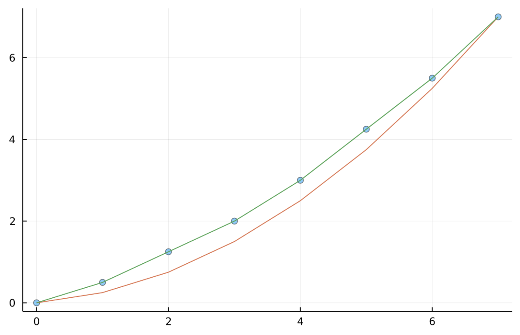
Figure 1. $\operatorname{NP}(f)$ for $f(x)=x^{8}+x^{6}+x^{2}$

Proposition 4.6.

The $p$-adic Newton polygon $\operatorname{NP}(f)$ has slopes (with multiplicities):

$$\{(0.5,1.0),(0.75,2.0),(1.0,1.0),(1.25,2.0),(1.5,1.0)\}.$$

Proof.

We know the $p$-adic valuation of the first four coefficients of the $C$-function by Proposition 4.5, noting that $\operatorname{ord}_{p}{C}_{0}=0$. Using the Hodge polygon, above in red, we can get a lower bound for the remaining coefficients, and so we see that the first three slopes must be $\frac{1}{2}$, $\frac{3}{4}$ and $\frac{3}{4}$. The fourth slope was already known to be $1$, and so by symmetry, the remaining slopes are as claimed. ∎

4.2. The Case $\lambda=\xi+2$

When $\lambda=\xi+2$, a key difference that occurs is that the action of $\tau$ on the matrix $\phi$ is nontrivial. Observe

$$(\phi)_{i,j}=\sum_{k=1}^{\infty}F_{pi-k}(\hat{\lambda}\pi)\tau F_{pk-j}(\hat{\lambda}\pi)=\sum_{k=1}^{\infty}F_{pi-k}(\hat{\lambda}\pi)F_{pk-j}(\hat{\lambda}^{p}\pi).$$

Lemma 4.7.

Let $w\in\mathbb{C}_{p}$ be a root of $x^{p-1}+1$. For $b,c$ positive integers with $b+c$ odd:

$$w^{b+pc}+w^{c+pb}=0.$$

Proof.

It is clear that $w^{b+pc}+w^{c+pb}=w^{b+c}(w^{(p-1)c}+w^{(p-1)b})$. But because $b+c$ is odd, we can without loss of generality take $c$ to be odd and $b$ to be even, so then:

$$w^{(p-1)c}+w^{(p-1)b} =(w^{p-1})^{2k+1}+(w^{p-1})^{2k^{\prime}}=(-1)^{2k+1}+(-1)^{2k^{\prime}}$$

$$=-1+1=0,$$

since $w$ satisfies $w^{p-1}+1=0$. ∎

For a product of power series $G=g_{1}\cdots g_{k}$ we refer to the $(r_{1},\cdots,r_{k})$-monomial, $[g_{1}\cdots g_{k}]_{(r_{1},\cdots,r_{k})}$, as the monomial obtained from the product $G$ by taking the $r_{1}$-power term from $g_{1}$, the $r_{2}$-power term from $g_{2}$, etc.

Lemma 4.8.

Let $G(x),H(x)\in\mathbb{Q}_{q}[[x]]$. Then the sum $G(\hat{\lambda}x)H(\hat{\lambda}^{p}x)+G(\hat{\lambda}^{p}x)H(\hat{\lambda}x)$ has only even powers of $x$.

Proof.

Write $G(x)=\sum_{k=0}^{\infty}G_{k}x^{k}$ and $H(x)=\sum_{k=0}^{\infty}H_{k}x^{k}$. For $r_{1},r_{2}\geq 1$ with $r_{1}+r_{2}$ odd, we compute that

$$[G(\hat{\lambda}x)H(\hat{\lambda}^{p}x)]_{(r_{1},r_{2})} +[G(\hat{\lambda}^{p}x)H(\hat{\lambda}x)]_{(r_{1},r_{2})}$$

$$=G_{r_{1}}\hat{\lambda}^{r_{1}}x^{r_{1}}H_{r_{2}}\hat{\lambda}^{pr_{2}}x^{r_{2}}+G_{r_{1}}\hat{\lambda}^{pr_{1}}x^{r_{1}}H_{r_{2}}\hat{\lambda}^{r_{2}}x^{r_{2}}$$

$$=(\hat{\lambda}^{r_{1}+pr_{2}}+\hat{\lambda}^{r_{2}+pr_{1}})G_{r_{1}}H_{r_{2}}x^{r_{1}+r_{2}}$$

$$=0,$$

where the last equality follows from Lemma 4.7 and the fact that $\hat{\lambda}^{p-1}+1=0$. ∎

Proposition 4.9.

For $k\geq 1$, $\operatorname{Tr}(\phi^{k})$ has only even powers of $\pi$.

Proof.

Fix $k\geq 1$. Just as in the proof of Lemma 4.2,

$$(\phi^{k})_{i,i}=\sum_{\begin{subarray}{c}w_{1},\cdots,w_{k-1}\geq 1\\ w_{0}=w_{k}=i\end{subarray}}\prod_{\ell=1}^{k}\left(\sum_{v=1}^{\infty}F_{pw_{\ell-1}-v}(\lambda\pi)F_{pv-w_{\ell}}(\lambda^{p}\pi)\right),$$

and so

$$\operatorname{Tr}\phi^{k}=\sum_{i=1}^{\infty}\sum_{w_{1},\cdots,w_{k-1}\geq 1}\prod_{\ell=1}^{k}\left(\sum_{v=1}^{\infty}F_{pw_{\ell-1}-v}(\lambda\pi)F_{pv-w_{\ell}}(\lambda^{p}\pi)\right).$$

Expanding $\operatorname{Tr}A^{k}$, each monomial comes from a product of the form:

$$T=\prod_{j=1}^{k}F_{pw_{j-1}-v_{j}}(\lambda\pi)F_{pv_{j}-w_{j}}(\lambda^{p}\pi),$$

some $v_{1},\cdots,v_{k}\geq 1$ and $w_{0},\cdots,w_{k}\geq 1$, with $w_{0}=w_{k}=i$ and $i\geq 1$.

Say we have a $(r_{1},\cdots,r_{2k})$-monomial coming from a product

$$\prod_{j=1}^{k}F_{pw_{j-1}-v_{j}}F_{pv_{j}-w_{j}},$$

some fixed $w_{j}$, $v_{j}$ and $i$. Define a new set of indices $w_{j}^{\prime}=v_{j}$ and $v_{j}^{\prime}=w_{j-1}$. These indices yield a product:

$$T^{\prime}=\prod_{j=1}^{k}F_{pv_{j-1}-w_{j-1}}(\lambda\pi)F_{pw_{j-1}-v_{j}}(\lambda^{p}\pi).$$

Define $G(x)=\prod_{j=1}^{k}F_{pv_{j-1}-w_{j-1}}(x)$ and $H(x)=\prod_{j=1}^{k}F_{pw_{j-1}-v_{j}}(x)$. Then, by Lemma 4.8, adding the $(r_{1},\cdots,r_{2k})$-monomial from $T$ to the $(r_{2k},r_{1},\cdots,r_{2k-1})$-monomial of $T^{\prime}$ yields zero, and the proposition follows. ∎

To see this explicitly, if we compute the traces of $\phi$ and its powers when $\lambda=\xi+2$, all the odd powers of $\pi$ collapse.

Lemma 4.10.

When $\lambda=\xi+2$,

$$\operatorname{Tr}(\phi) \equiv 3\pi^{2}+2\pi^{4}\bmod p$$

$$\operatorname{Tr}(\phi^{2}) \equiv 24\pi^{4}+12\pi^{6}+16\pi^{8}\bmod p^{2}$$

$$\operatorname{Tr}(\phi^{3}) \equiv 57\pi^{6}+124\pi^{8}+85\pi^{10}+98\pi^{12}\bmod p^{3}$$

Proof.

See proof of Lemma 4.4. ∎

Lemma 4.11.

We have $\operatorname{ord}_{p}{C}_{1}=\frac{1}{2}$, $\operatorname{ord}_{p}{C}_{2}=2$ and $\operatorname{ord}_{p}{C}_{3}=3$.

Proof.

Just like Lemma 4.5, this is a direct computation following from Lemma 4.3 and Lemma 4.11. ∎

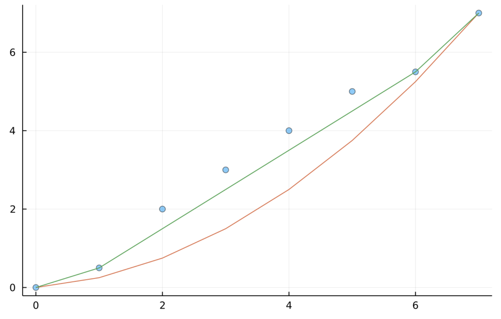
Figure 2. $\operatorname{NP}(\lambda f)$ for $f=x^{8}+x^{6}+x^{2}$, $\lambda=\xi+2$

Proposition 4.12.

When $\lambda=\xi+2$, the Newton polygon $\operatorname{NP}(\lambda f)$ has $p$-adic slopes (with multiplicities):

$$\{(0.5,1.0),(1.0,5.0),(1.5,1.0)\}.$$

Proof.

We know $\operatorname{ord}_{p}{C}_{1}$, $\operatorname{ord}_{p}{C}_{2}$ and $\operatorname{ord}_{p}{C}_{3}$ by Lemma 4.11 and that $\alpha_{4}=1$. Putting this all together just as we did in Proposition 4.6 yields the Newton polygon. ∎

5. Counting Points in $\mathbb{F}_{p^{a}}^{\times}$

This section is independent of the rest of the paper and will be used to obtain an upper bound for the number of possible Newton polygons based solely on some combinatorics in $\mathbb{F}_{p^{a}}^{\times}$.

Let $q=p^{a}$ and define $\overset{\sim}{\mathbb{F}}_{q}$ to be the set of elements of $\mathbb{F}_{q}^{\times}$ modulo the equivalence relations:

1. $x\sim y$ if $x^{p-1}=y^{p-1}$, and

2. $x\sim y$ if $x^{p^{i}}=y$ for some $i\geq 0$ (i.e. $x$ and $y$ are Galois conjugates).

The goal is this section will be to count the number of equivalence classes in $\overset{\sim}{\mathbb{F}}_{q}$.

For $x\in\mathbb{F}_{q}^{\times}$, define $\deg x$ to be the degree of the minimal polynomial of $x$. Explicitly, $\deg x$ is the minimal integer $i$ such that $x,x^{p},x^{p^{2}},\cdots,x^{p^{i-1}}$ are each unique:

$$\deg x=\min_{0<i\leq a}(x^{p^{i}-1}=1).$$

Consider the quotient group of $\mathbb{F}_{q}^{\times}$,

$$\mathbb{F}_{q}^{\times,p-1}=\mathbb{F}_{q}^{\times}/\mathbb{F}_{p}^{\times},$$

consisting of cosets whose elements have the same value when taken to the $(p-1)$-power. Our first step will be to show that within each coset in $\mathbb{F}_{q}^{\times,p-1}$, the degree of each element is the same.

Lemma 5.1.

Let $x,y\in\mathbb{F}_{p^{a}}^{\times}$ such that $x^{p-1}=y^{p-1}$. Then $\deg x=\deg y$.

Proof.

Let $k=\deg x$ and $\ell=\deg y$ and suppose that $k>\ell$. Then $y^{p^{\ell}}=y$ and:

$$x =x^{p^{k}}=x^{p^{k}-1}x=(x^{p-1})^{\frac{p^{k}-1}{p-1}}x=(y^{p-1})^{\frac{p^{k}-1}{p-1}}x=y^{p^{k}-1}x$$

$$=y^{p^{k}}\cdot\frac{x}{y}=(y^{p^{\ell}})^{p^{k-\ell}}\cdot\frac{x}{y}=y^{p^{k-\ell}-1}\cdot x=(y^{p-1})^{\frac{p^{k-\ell}-1}{p-1}}\cdot x$$

$$=(x^{p-1})^{\frac{p^{k-\ell}-1}{p-1}}x=x^{p^{k-\ell}}.$$

But this is a contradiction since the degree of $x$ is minimal. ∎

Thus, if we take a coset $(x_{1},\cdots,x_{p-1})\in\mathbb{F}_{q}^{\times,p-1}$, each element $x_{i}$ has the same degree, say $n$, and we can write:

$$x_{1},x_{1}^{p}, \cdots,x_{1}^{p^{n-1}}$$

$$x_{2},x_{2}^{p}, \cdots,x_{2}^{p^{n-1}}$$

$$\vdots$$

$$x_{p-1},x_{p-1}^{p}, \cdots,x_{p-1}^{p^{n-1}},$$

where each row has distinct elements of $\mathbb{F}_{q}^{\times}$ by Lemma 5.1. Observe first that each column is also a coset of $\mathbb{F}_{q}^{\times,p-1}$ since for any $i,j,k$,

$$(x_{i}^{p^{k}})^{p-1}=(x_{i}^{p-1})^{p^{k}}=(x_{j}^{p-1})^{p^{k}}=(x_{j}^{p^{k}})^{p-1}.$$

Second, by the equivalence relations defining $\overset{\sim}{\mathbb{F}}_{q}$, all of these elements are part of the same equivalence class of $\overset{\sim}{\mathbb{F}}_{q}$. Thus, if we know how many columns are distinct, we can determine how many elements are part of the same equivalence class in $\overset{\sim}{\mathbb{F}}_{q}$.

To determine which of the columns are distinct, note that each column will have the same value when the elements in that column are taken to the $(p-1)$-power. Thus, if we define

$$\lambda_{i}=(x_{1}^{p^{i}})^{p-1}=x_{1}^{(p-1)p^{i}},$$

with $0\leq i\leq n-1$, the columns with distinct elements will have different values of $\lambda_{i}$. Since the order of the columns above are invariant up to a shifting operator, we can, without loss of generality, suppose that if two columns repeat, it is the first and $k$th ones. In this case, we find that $x^{p-1}=x^{(p-1)p^{k}}$, and

$$0 =x^{(p-1)(p^{k}-1)}-x^{p-1}=x^{p-1}(x^{(p-1)(p^{k}-1)}-1),$$

so that if $x$ is such that $\lambda_{0}=\lambda_{k}$, it must be a solution to $x^{(p-1)(p^{k}-1)}=1$ for some $k\geq 1$. Furthermore, by substituting $x\mapsto x^{p^{\ell}}$, some $\ell\geq 1$, we see that $x^{(p-1)p^{\ell}}=x^{(p-1)p^{k+\ell}}$. Thus, for any $i,j\geq 0$,

$$\lambda_{i}=\lambda_{i+k}=\lambda_{i+2k}=\cdots=\lambda_{i+jk\bmod\ n}.$$

This argument leads to the following lemma:

Lemma 5.2.

For any $x\in\mathbb{F}_{q}^{\times}$ with $\deg x=n$, there are exactly $\deg x^{p-1}$-many distinct values in the set $\{x^{p-1},(x^{p})^{p-1},\cdots,(x^{p^{n-1}})^{p-1}\}$.

Example.

Let $p=5,a=4$ and $\mathbb{F}_{q}^{\times}=\langle\xi\rangle$. Let $\omega=\xi^{2}+2\xi+2$ so that $(\omega_{1},\omega_{2},\omega_{3},\omega_{4})=(\omega,2\omega,3\omega,4\omega)$ is a coset in $\mathbb{F}_{q}^{\times,p-1}$.

In this case, we can compute that $\lambda_{1}=\lambda_{3}=4\xi^{3}+4\xi^{2}+4\xi+1$ and $\lambda_{2}=\lambda_{4}=\xi^{3}+\xi^{2}+\xi+1$ and:

$$\begin{matrix}\lambda_{1}&\lambda_{2}&\lambda_{3}&\lambda_{4}\\ \hline\cr\omega_{1}&\omega_{1}^{p}&\omega_{1}^{p^{2}}&\omega_{1}^{p^{3}}\\ \omega_{2}&\omega_{2}^{p}&\omega_{2}^{p^{2}}&\omega_{2}^{p^{3}}\\ \omega_{3}&\omega_{3}^{p}&\omega_{3}^{p^{2}}&\omega_{3}^{p^{3}}\\ \omega_{4}&\omega_{4}^{p}&\omega_{4}^{p^{2}}&\omega_{4}^{p^{3}}\\ \end{matrix}\ =\ \begin{matrix}\lambda_{1}&\lambda_{2}&\lambda_{1}&\lambda_{2}\\ \hline\cr\omega_{1}&\omega_{1}^{p}&\omega_{4}&\omega_{4}^{p}\\ \omega_{2}&\omega_{2}^{p}&\omega_{3}&\omega_{3}^{p}\\ \omega_{3}&\omega_{3}^{p}&\omega_{2}&\omega_{2}^{p}\\ \omega_{4}&\omega_{4}^{p}&\omega_{1}&\omega_{1}^{p}\\ \end{matrix}.$$

On the other hand, by Lemma 5.2, we obtain $\deg\omega_{1}^{p-1}=2$, which agrees with the above.

For $n\geq 0$ and $0<k\leq n$, define the subsets of $\mathbb{F}_{q}^{\times}$:

$$\Gamma_{n,k}=\{x\in\mathbb{F}_{q}^{\times}:\deg x=n,\deg x^{p-1}=k\}.$$

For example, when $k=n$, $\Gamma_{n,n}$ consists of all elements of $\mathbb{F}_{q}^{\times}$ such that each element in $\{x,x^{p},\cdots,x^{p^{n-1}}\}$ is distinct and $x^{(p-1)(p^{i}-1)}=1$ has no solution for $0<i<n$. Again, this latter condition can be also be given as every component in $(x^{p-1},x^{(p-1)p},\cdots,x^{(p-1)p^{n-1}})$ is unique.

Proposition 5.3.

The sets $\Gamma_{n,k}$ have the following properties:

1. If $n\nmid a$, then $\Gamma_{n,k}=\varnothing$ for any $k$.

2. If $k\nmid n$, then $F_{n,k}=\varnothing$.

3. If $n^{\prime}\neq n$ and $k\neq k^{\prime}$, then $\Gamma_{n,k}\cap\Gamma_{n^{\prime},k^{\prime}}=\varnothing$.

Proof.

1. Let $\Phi_{d}(x)$ be the $d$-th cyclotomic polynomial. It is well-known that $x^{n}-1=\prod_{d|n}\Phi_{d}(x)$. Thus if $n\mid a$,

   $$x^{n}-1=\prod_{d|n}\Phi_{d}(x)\mid\prod_{d|a}\Phi_{d}(x)=x^{a}-1.$$

   On the other hand, if $(x^{n}-1)\mid(x^{a}-1)$, then we must have $n|a$ since the cyclotomic polynomials are irreducible. The claim then follows because $x^{p^{n}-1}=1$ if and only if $(p^{n}-1)\mid(p^{a}-1)$. But this only occurs if and only if $n|a$.

2. Let $r=\gcd(k,n)$ so that by assumption $1\leq r<k$. If $x\in\Gamma_{n,k}$, we have $x^{p^{n}-1}=1$, where $n$ is minimal, and $x^{(p-1)(p^{k}-1)}=1$, with $k$ also minimal. By Bezout’s Lemma, there exist integers $i$ and $j$ such that $ik+jn=r$. Considering the sum $ik+jn\bmod n$, we can take $i$ and $j$ to both be positive integers. Note that because $x^{p^{n}}=x$,

   $$x^{(p-1)p^{r}}=x^{(p-1)p^{ik+jn}}=x^{(p-1)p^{ik}}.$$

   Then, since $x^{(p-1)(p^{k}-1)}=1$, $x^{(p-1)p^{k}}=x^{p-1}$ and therefore

   $$x^{(p-1)p^{ik}}=(x^{(p-1)p^{k}})^{p^{(i-1)k}}=(x^{p-1})^{p^{(i-1)k}}=x^{(p-1)p^{(i-1)k}}.$$

   Performing this repeatedly yields $x^{(p-1)p^{ik}}=x^{p-1}$, and hence $x^{(p-1)p^{r}}=x^{p-1}$. However, this is a contradiction since $r<k$ and $k$ is minimal.

3. This is clear from the definition of $\Gamma_{n,k}$.

∎

To compute the order of $\Gamma_{n,k}$, we first find all $x\in\mathbb{F}_{q}^{\times}$ such that

(2) $$x^{p^{n}-1}=1=x^{(p-1)(p^{k}-1)}.$$

Because not all of these values of $x$ satisfy (2) minimally, it is necessary to subtract all $x$ achieving (2) for $n^{\prime}<n$ and $k^{\prime}<k$. This is the content of Lemma 5.4 and Proposition 5.5 below.

Lemma 5.4.

The number of $x\in\mathbb{F}_{q}^{\times}$ such that $x^{p^{n}-1}=1$ and $x^{(p-1)(p^{k}-1)}=1$ is equal to $\gcd(p^{n}-1,(p-1)(p^{k}-1))$.

Proof.

In a cyclic group of order $N$, the number of $m$-th roots of unity is equal to $\gcd(N,m)$. Applying this to $\mathbb{F}_{q}^{\times}$ yields the lemma. ∎

Proposition 5.5.

For $n|a$,

$$|\Gamma_{n,n}|=n\cdot M_{n}-\sum_{k|n,k\neq n}|\Gamma_{n,k}|.$$

When $k\neq n$,

$$|\Gamma_{n,k}|=\gcd(p^{n}-1,(p-1)(p^{k}-1))-\sum_{\begin{subarray}{c}d|n,\\ j|d\textrm{ and }j|k\end{subarray}}|\Gamma_{d,j}|.$$

Proof.

Consider the $k=n$ case first. In this case, it is well-known that the number of irreducible polynomials of of degree $n$ over $\mathbb{F}_{q}$ is given by the $n$-th necklace polynomial $M_{n}$:

$$M_{n}=\frac{1}{n}\sum_{d|n}\mu(d)p^{n/d},$$

where $\mu(d)$ is the Möbius function. Thus, the number of elements of degree $n$ in $\mathbb{F}_{q}^{\times}$ is $nM_{n}$. If we subtract off all $\Gamma_{n,k}$ with $k\mid n$, we will remove all possible $x$ with $\deg x^{p-1}<n$, and the claim follows.

For $k\neq n$, by Lemma 5.4, $\gcd(p^{n}-1,(p-1)(p^{k}-1))$ is the number of points in $\mathbb{F}_{p^{a}}^{\times}$ such that $x^{p^{n}}=1$ and $x^{(p-1)(p^{k}-1)}=1$. From this we need to remove all points satisfying $x^{p^{n^{\prime}}}=1$ and $x^{(p-1)(p^{k^{\prime}}-1)}=1$ for $n^{\prime}<n$ or $k^{\prime}<k$. By Proposition 5.3, these are exactly all $d$ with $d|n$ and all $j$ with $j|d$ and $j|k$. ∎

Example.

Let $p$ and $a$ both be primes such that $\gcd(p-1,1+\cdots+p^{a-1})=1$. Then for $x\in\mathbb{F}_{q}^{\times}$, either $x\in\mathbb{F}_{p}^{\times}$ or $x$ satisfies an irreducible polynomial of degree $a$. By Proposition 5.3, we immediately see that all the $\Gamma_{n,k}$ are empty except possibly:

$$\Gamma_{a,a},\Gamma_{a,1},\Gamma_{1,1}.$$

But if $x\in\Gamma_{a,1}$, then by Lemma 5.4 and our assumption on $p$ and $a$, there are at most

$$\gcd(p^{a}-1,(p-1)^{2})=(p-1)\gcd(1+\cdots+p^{a-1},p-1)=p-1$$

many $x\in\mathbb{F}_{q}^{\times}$ that are potentially in $\Gamma_{a,1}$. But these are just the elements of $\mathbb{F}_{p}^{\times}$ and so $\Gamma_{a,1}$ must be empty. Then, $\Gamma_{1,1}=\mathbb{F}_{p}^{\times}$ and $\Gamma_{a,a}=\mathbb{F}_{q}^{\times}-\mathbb{F}_{p}^{\times}$. The elements of $\Gamma_{1,1}$ are their own class in $\overset{\sim}{\mathbb{F}}_{q}$, so it amounts to classify $\Gamma_{a,a}$.

By definition of $\Gamma_{a,a}$, the elements in the cosets have distinct values when taken to their $(p-1)$-powers:

$$\begin{matrix}\lambda_{1}&\lambda_{2}&\cdots&\lambda_{a}\\ \hline\cr\omega_{1}&\omega_{1}^{p}&\cdots&\omega_{1}^{p^{a-1}}\\ \omega_{2}&\omega_{2}^{p}&\cdots&\omega_{2}^{p^{a-1}}\\ &&\vdots&\\ \omega_{p-1}&\omega_{p-1}^{p}&\cdots&\omega_{p-1}^{p^{a-1}},\\ \end{matrix}$$

where all the $\lambda_{i}$ are distinct. Hence, the number of these elements in $\overset{\sim}{\mathbb{F}}_{q}$ can be given by:

$$\frac{|\mathbb{F}_{q}^{\times}|-|\mathbb{F}_{p}^{\times}|}{a(p-1)}=\frac{(p-1)(1+\cdots+p^{a-1})-(p-1)}{a(p-1)}=\frac{p+\cdots+p^{a-1}}{a},$$

and so the total number of classes in $\overset{\sim}{\mathbb{F}}_{q}$ is:

$$|\overset{\sim}{\mathbb{F}}_{q}|=\frac{p+\cdots+p^{a-1}}{a}+1.$$

We can generalize the above example to computing the total number of equivalence classes in each $\Gamma_{n,k}$, and therefore the number of classes in $\overset{\sim}{\mathbb{F}}_{q}$:

Proposition 5.6.

The number of classes of $\overset{\sim}{\mathbb{F}}_{q}$ is bounded above by:

$$|\overset{\sim}{\mathbb{F}}_{q}|\leq\frac{1}{p-1}\sum_{n|a}\sum_{k|n}\frac{1}{k}|\Gamma_{n,k}|.$$

Proof.

Fix $n\mid a$. We can compute the number of unique elements within each set $\Gamma_{n}$ by computing the number of elements in each $\Gamma_{n,k}$ and dividing by the number of unique $\lambda_{i}$’s for each $k$. For $k\mid n$, as in Example Example and by Lemma 5.2 we just get $\frac{1}{k(p-1)}\Gamma_{n,k}$-many classes, and the computation follows from the fact that $\overset{\sim}{\mathbb{F}}_{q}$ is the disjoint union of all $\Gamma_{n}=\cup_{k|n}\Gamma_{n,k}$ for $n\mid a$. ∎

6. The General Case

In this section we provide an upper bound for the number of possible Newton polygons arising as $\lambda$ varies and pose some questions for future study.

Before we can prove the main upper bound, we need one more condition under which the Newton polygons coincide.

Proposition 6.1.

Let $\lambda\in\overline{\mathbb{F}_{p}^{\times}}$.Then $\operatorname{NP}(\lambda f)=\operatorname{NP}(\lambda^{p}f)$.

Proof.

By Lemma 3.2, $\phi_{\lambda f}(\pi)=\pi_{f}(\hat{\lambda}\pi)$. So say $\lambda,\lambda^{\prime}\in\mathbb{F}_{p^{a}}^{\times}$ such that $\tau\lambda=\lambda^{\prime}$, that is, $\hat{\lambda}=\hat{\lambda}^{\prime p}$. Then:

$$\phi_{\lambda f}(\pi) =\prod_{i=1}^{a-1}\tau^{-i}M_{f}(\hat{\lambda}\pi)=\prod_{i=1}^{a-1}M_{f}(\tau^{-i}(\hat{\lambda})\pi)=\prod_{i=1}^{a-1}M_{f}(\hat{\lambda}^{p^{i}}\pi)$$

$$=\prod_{i=1}^{a-1}M_{f}(\hat{\lambda}^{\prime p^{i+1}}\pi)=\prod_{i=1}^{a-1}M_{f}(\hat{\lambda}^{\prime p^{i}}\pi)=\phi_{\lambda^{\prime}f}(\pi).$$

Applying this iteratively, we see that if $\lambda=\lambda^{\prime p^{k}}$, some $k$, then $\phi_{\lambda f}(\pi)=\phi_{\lambda^{\prime}f}(\pi)$. Hence $\operatorname{NP}(\lambda f)=\operatorname{NP}(\lambda^{\prime}f)$. ∎

Theorem 6.2.

For any $f(x)$ over $\mathbb{F}_{p^{a}}$, the number of unique Newton polygons in the family $\mathcal{N}_{f}=\{\operatorname{NP}(\lambda f)\}_{\lambda\in\mathbb{F}_{q}^{\times}}$, is bounded above by:

$$|\mathcal{N}_{f}|\leq\frac{1}{p-1}\sum_{n|a}\sum_{k|n}\frac{1}{k}|\Gamma_{n,k}|.$$

Proof.

By Proposition 3.3 and Proposition 6.1, we see that the number of distinct Newton polygons is bounded above by $|\overset{\sim}{\mathbb{F}}_{q}|$. But by Proposition 5.6, this is exactly the bound above. ∎

As one more application, observe that in the example worked out in Section 4, all $\lambda$ changing the Newton polygon from the base case of $\operatorname{NP}(f)$ are roots of a polynomial in $\mathbb{F}_{p}[X]$, $X^{p-1}-1$. For general $f(x)$, this phenomena continues to hold, and we see that to each distinct Newton polygon there exists a polynomial in $\mathbb{F}_{p}[x]$ whose roots yields the same Newton polygon $\operatorname{NP}(\lambda f)$.

As in Theorem 6.2, let $\mathcal{N}_{f}=\{\operatorname{NP}(\lambda f)\}_{\lambda\in\mathbb{F}_{p^{a}}^{\times}}$ be the set of Newton polygons as $\lambda$ varies and write $\mathcal{N}_{f}=\{N_{i}\}_{i=1}^{k}$, some $k\geq 1$, be the set of unique Newton polygons coming from the variation.

Proposition 6.3.

For each Newton polygon $N_{i}$, let $G_{i}$ be the set of all $\lambda\in\mathbb{F}_{q}^{\times}$ such that $\operatorname{NP}(\lambda f)=N_{i}$. Then, $g_{i}(X)=\prod_{\lambda\in G_{i}}(X-\lambda)\in\mathbb{F}_{p}[X]$.

Proof.

By Proposition 6.1, we can break up $G_{i}$ into $\tau$-invariant subsets. For $\lambda\in G_{i}$, define the polynomial

$$g_{\lambda}(x)=\prod_{\begin{subarray}{c}\lambda^{\prime}|\\ \lambda^{\prime p^{k}}=\lambda,k\geq 1\end{subarray}}(x-\lambda^{\prime}),$$

and note that $g_{\lambda}$ is $\tau$-invariant by definition, which implies that it lies in $\mathbb{F}_{p}[x]$. Write $G_{i}=G_{i,1}\cup\cdots\cup G_{i,m_{i}}$, some $m_{i}\geq 1$ and $G_{i,j}$ such that each $G_{i,j}$ is closed taking $p$-powers. Take $[G_{i}]$ to be a set of representatives from each class $G_{i,j}$ and observe that

$$g_{i}=\prod_{\lambda\in G_{i}}(x-\lambda)=\prod_{\lambda\in[G_{i}]}g_{\lambda}.$$

But then $g_{\lambda}\in\mathbb{F}_{q}[x]$, so we must also have $g_{i}\in\mathbb{F}_{p}[x]$.

∎

We end this section with a couple questions.

Question 1.

Is the bound in Theorem6.2 sharp?

For example, when $p=5$, $a=2$, the bound in Theorem 6.2 tells us that there are at most four distinct Newton polygons in $\{\operatorname{NP}(\lambda)\}_{\lambda\in\mathbb{F}_{q}^{\times}}$. When $f(x)=x^{11}+x^{7}+x$, we see, writing $\mathbb{F}_{q}^{\times}=\langle\xi\rangle$, that there are three distinct Newton polygons occurring at $\lambda=1$, $\xi$ and $\xi+2$. We have not found any examples obtaining the bound.

Question 2.

For each $f(x)\in\mathbb{F}_{q}[x]$, prime $p$ and $a\geq 1$, does there exist a $\lambda_{p,a}\in\mathbb{F}_{q}^{\times}$ such that

$$\frac{|\{\mu\in\mathbb{F}_{q}^{\times}|\operatorname{NP}(\mu f)\neq\operatorname{NP}(\lambda_{p,a}f)\}|}{|\{\mu\in\mathbb{F}_{q}^{\times}|\operatorname{NP}(\mu f)=\operatorname{NP}(\lambda_{p,a}f)\}|}\to 0\textrm{ as }p\textrm{ or }a\to\infty.$$

Fundamentally, Question 2 asks whether or not there exists a “most common” Newton polygon as $\lambda$ varies. In cases we have computed, the Newton polygon does not appear to change very frequently when $f$ is multiplied by some $\lambda$, and so we conjecture that as the size of the field $\mathbb{F}_{q}^{\times}$ becomes larger, most of the Newton polygons $\operatorname{NP}(\lambda f)$ are the same.

References

[1]
Maurizio Boyarsky,
The Reich trace formula,
Astérisque119-120 (1984), 129–139.
[2]
Neal Koblitz,
-adic Numbers, -adic Analysis, and Zeta-functions,
Springer-Verlag, New York, 1984.
[3]
Alan Lauder and Daqing Wan,
Computing zeta functions of Artin-Schreier curves over finite fields,
Journal of Complexity5 (2004), 35–55.
[4]
Daqing Wan,
Exponential Sums over Finite Fields,
Journal of Systems Science and Complexity34 (2021), 1225–1278.
[6]
Bezanson, J., Edelman, A., Karpinski, S., Shah, V.B.,
Julia: a fresh approach to numerical computing,
SIAM Rev.59(1) (2017), 65–98.
[7]
Claus Fieker, William Hart, Tommy Hofmann, and Fredrik Johansson,
Nemo/Hecke: computer algebra and number theory packages for the Julia programming language,
ISSAC’17—Proceedings of the 2017 ACM International Symposium on Symbolic and Algebraic Computation, 157–164.
ACM, New York (2017).
[8]
Hui June Zhu,
-adic Variation of -Functions of One variable Exponential Sums, I,
American Journal of Math.125(3) (2003), 669–690.