A soft and transient ultraluminous X-ray source with 6-h modulation in the NGC 300 galaxy

We investigate the nature of CXOU J005440.5-374320 (J0054), a peculiar bright ($\sim$$4\times 10^{39}$ erg s^-1) and soft X-ray transient in the spiral galaxy NGC 300 with a 6-hour periodic flux modulation that was detected in a 2014 Chandra observation. Subsequent observations with Chandra and XMM–Newton, as well as a large observational campaign of NGC 300 and its sources performed with the Swift Neil Gehrels Observatory, showed that this source exhibits recurrent flaring activity: four other outbursts were detected across $\sim$8 years of monitoring. Using data from the Swift/UVOT archive and from the XMM–Newton/OM and Gaia catalogues, we noted the source is likely associated with a bright blue optical/ultraviolet counterpart. This prompted us to perform follow-up observations with the Southern African Large Telescope in December 2019. With the multi-wavelength information at hand, we discuss several possibilities for the nature of J0054. Although none is able to account for the full range of the observed peculiar features, we found that the two most promising scenarios are a stellar-mass compact object in a binary system with a Wolf–Rayet star companion, or the recurrent tidal stripping of a stellar object trapped in a system with an intermediate-mass ($\sim$1000 M_⊙) black hole.

1 Introduction

The Chandra ACIS Timing Survey at Brera And Roma astronomical observatories (CATS @ BAR) is a systematic search for coherent periodic signals in Chandra/ACIS archival data in Timed Exposure mode. The first catalog of new pulsators was published in Israel et al. (2016) and several sources were studied individually (Esposito et al., 2013b, c, a, 2015; Bartlett et al., 2017; Sidoli et al., 2016, 2017). Over 50 new X-ray pulsators were discovered so far.

CXOU J005440.5–374320 (J0054 for brevity) was discovered in the CATS @ BAR project with a large-amplitude flux modulation at a period of $\sim$6 h. It is seen projected in the sky inside the inner region of the NGC 300 (Fig. 1), a face-on spiral galaxy (Scd) in the Sculptor group at a Cepheid distance of 1.88 Mpc (Gieren et al., 2005, corresponding to a distance modulus of 26.4 mag).

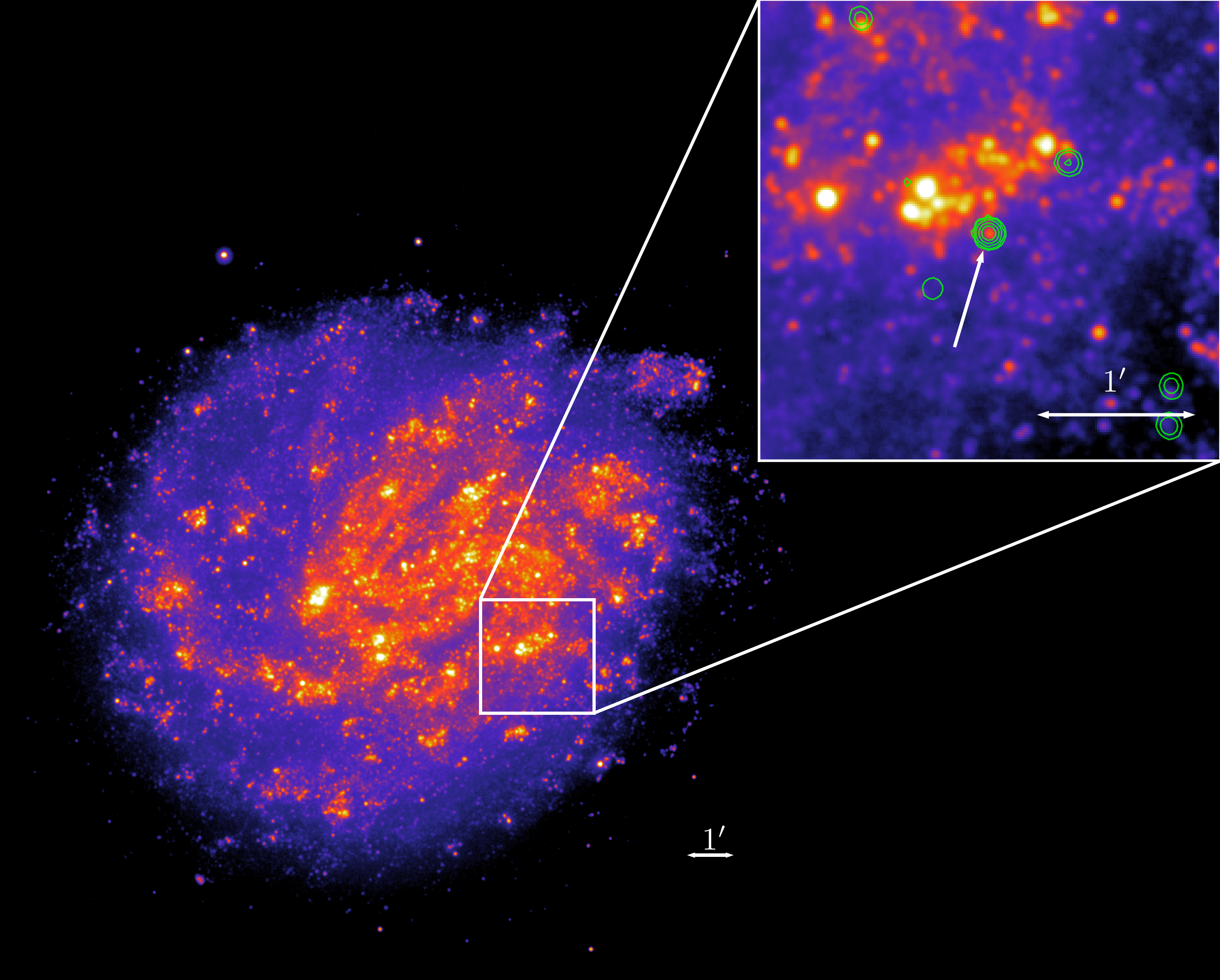
Figure 1: NGC 300 from Swift/UVOT in the UVW2 band. The inset shows the location of J0054, which is indicated by the white arrow. X-ray contours from the Chandra detection of November 2014 are plotted in green.

NGC 300, due to its proximity and favourable inclination, has been the subject of many studies about its stellar populations (Bresolin et al., 2009, and references therein), star formation history (Butler et al., 2004), Wolf–Rayet (WR) stars and OB associations (Schild et al., 2003; Pietrzyński et al., 2001), planetary nebulae (Peña et al., 2012), variable stars (Pietrzyński et al., 2002; Mennickent et al., 2004), dust content (Helou et al., 2004; Roussel et al., 2005), X-ray sources (Read & Pietsch, 2001; Carpano et al., 2005; Binder et al., 2017; Carpano et al., 2018; Urquhart et al., 2019), supernova remnants (Blair & Long, 1997; Pannuti et al., 2000; Payne et al., 2004; Gross et al., 2019), and UV emission properties (Muñoz-Mateos et al., 2007). NGC 300 has been therefore observed with a wide variety of different telescopes and a large amount of multiwavelength data is available.

In this work, we focus on the nature of J0054. In Section 2, we present the data sets and the observational properties of the source, highlighting its X-ray behaviour and its optical/UV counterpart. In Section 3 we discuss possible scenarios which could originate J0054 emission and make our concluding remarks.

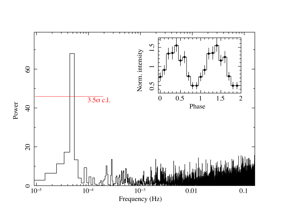
Figure 2: Timing analysis of J0054. Left panel: Fourier power spectrum of the Chandra data of J0054. The red line indicates the local 3.5$\sigma$ detection threshold adopted in the CAT @ BAR project. The prominent peak well above the threshold ( 5.9$\sigma$) corresponds to the $\sim$6 h modulation of J0054. The inset shows the pulse profile obtained by folding the data at the best period of $5.88\pm 0.12$ h. Right panel: Light curve (the background is negligible). The bin time is 2500 s.

2 Observational properties

2.1 X-ray data sets

2.1.1 Chandra

J0054 fell into Chandra field of view four times, see Tab. LABEL:tab:cxo. Data were reprocessed and reduced with the Chandra Interactive Analysis of Observations software package (CIAO, v.4.12; Fruscione et al. 2006) and the CALDB 4.9.0 release of the calibration files. In the first two visits, the source was not detected and $3\sigma$ upper limits on its flux were obtained with the CIAO tool srcflux , following the default Bayesian approach. In the two most recent observations, the source is located at 3.7 and 6 arcmins from the telescope aim point, respectively. The source counts were extracted from elliptical regions with semi-major and semi-minor axes of 3.2 and 2.6 arcseconds for the November 2014 observation, and of 5 and 4 arcseconds for the April 2020 observation, corresponding to a point-spread function (PSF) fraction of about 96%. Backgrounds were estimated from source-free annular regions, centred on the source position, of 10 and 20 arcseconds radii.

2.1.2 Swift/XRT

Owing to the large monitoring campaign brought forth on NGC 300 and its sources, the location of J0054 was in the Swift/XRT field of view on numerous occasions (170 times by the end of 2022) across a span longer than 15 years, but it was detected only in four visits: in August 2018, January 2019, April 2020, and one last time in September 2020, as reported in Tab. LABEL:tab:cxo. Count rates, and $3\sigma$ upper limits for all the observations in which the source is not detected, were extracted using the ximage tool sosta , following the default Poissonian approach (a Bayesian approach was also tested and it provided slightly deeper upper limits, still however compatible with the Poissonian ones). Merging together all Swift–XRT non-detections, the total exposure time amounts to $\approx 570$ ks, but the source still cannot be detected. The $3\sigma$ upper limit on the stacked observation is $8.05\times 10^{-5}$ cts s^-1, corresponding to a flux limit of $2.2\times 10^{-15}$ erg cm^-2 s^-1 (assuming the best fitting model described below).

2.1.3 XMM–Newton

The position of J0054 was imaged with XMM–Newton seven times, as reported in Tab. LABEL:tab:cxo, but the source was never detected. For each observation, data were retrieved from the XMM–Newton science archive and reduced following the standard procedure. The $3\sigma$ upper limits were obtained from the EPIC-pn cameras, with the sole exception of the fourth observation, in which the source falls on the EPIC-pn’s border and hence data from the merged EPIC-MOS cameras were used. The merging of the MOS cameras was performed with the sas tool merge. The $3\sigma$ upper limits were obtained with the eupper tool, from a circular region of 15” radius centred on J0054 position, with background counts extracted from a nearby free-of-sources circular region of 30” radius on the same detector chip , following the default Bayesian approach.

2.2 Short-term variability

The CATS @ BAR pipeline detected the uncatalogued X-ray source J0054 in a $\approx$60 ks exposure carried out in November 2014 (Table LABEL:tab:cxo) and singled it out as a new X-ray pulsator with a $\sim$6 h flux modulation (Fig. 2). Taking into account the 16 377 independent trials, the false alarm probability was $\sim$$7.6\times 10^{-11}$, which corresponds to a 6.5$\sigma$ detection. After correcting for the (mild) red noise in the exposure following Israel & Stella (1996), we evaluated the significance of the signal at $5.9\sigma$. Due to the relatively poor statistics, the approach of using the light curve to estimate the significance of modulation is not recommended and results in an underestimation of the real statistical level. Nonetheless, as an additional test, we compared the fit of the lightcurve with a constant and a constant plus a sinusoidal component. This comparison gives a F-test probability of $5\sigma$ that the addition of the sinusoid is significant.

As a further test, we also simulated 10⁵ Fourier power spectra with the same properties as that of Chandra ( a Poissonian noise plus a $f^{-\alpha}$ additional component, where $\alpha=0.71\pm 0.05$ is inferred by fitting the power spectra distribution continuum of the original Chandra dataset) and verified that no significant peak was detected by the used detection algorithm (which takes into account for any additional non-Poissonian noise component) at frequencies shorter than 10^-3 Hz, setting a probability threshold of 10^-5 ($>$ 4.4$\sigma$) at the 5.88h-period frequency. The above numbers are consistent with the 5$\sigma$ and the 5.9$\sigma$ level inferred by using two different independent approaches. Correspondingly, we conclude that the signal significance is larger than $>4.4\sigma$ and likely lies in the 5–5.9$\sigma$ range.

From the fit of the sinusoidal function, we derived a period of $P=5.88\pm 0.12$ h, which is entirely consistent with that reported in Israel et al. (2016). The pulsed fraction, estimated from the semi-amplitude of the sinusoidal function, was $52\pm 4$%. With a $\nu/\Delta\nu$ factor of $\sim$10, the signal is seemingly coherent (that is, strictly periodic), but this is something clearly difficult to assess when only a few cycles are sampled, and a quasi-periodic modulation cannot be excluded.

In the last Chandra visit, no significant pulsation was detected, although the 3$\sigma$ upper limit on the pulsed fraction is about 50%. In the four Swift/XRT detections, the signal-to-noise ratio is too low to carry out a meaningful timing analysis.

2.3 Long-term variability

Owing to the long-term monitoring of NGC 300, we can trace J0054 X-ray variability across more than two decades (an early 1990s ROSAT upper limit is unfortunately too shallow to be relevant in this regard). J0054 was never detected before the Chandra pointing of November 2014 (Obs.ID 16029). The closest observation is the non-detection by Chandra, six months earlier, in May 2014 (Obs.ID 16028). The $3\sigma$ upper limit obtained in May 2014 implies a flux variation of at least a factor of 100. After this, J0054 has not been pointed for $\sim$1.5 years and when NGC 300 was observed again, it had disappeared: it is not detected in three short observations by Swift/XRT in April 2016 (although the upper limits for these observations are very shallow), nor in two longer observations by XMM–Newton at the end of the same year. J0054 reappeared in a Swift/XRT observation in late August 2018, unfortunately, the upper limits around this detection are too shallow to reconstruct the detailed source behaviour. The scene repeated on January 2019, April 2020 and September 2020. In April 2020 J0054 has been detected by both Swift/XRT (Obs.ID 00095672001) and Chandra (Obs.ID 22375) less than ten days apart. After September 2020, J0054 has never been detected again, possibly also due to the visits on NGC 300 growing sparser and shallower with time. Fig. 3 shows the long-term light curve of J0054 in the years from approximately 2000 to 2023, count-rates were converted into fluxes with the model described below.

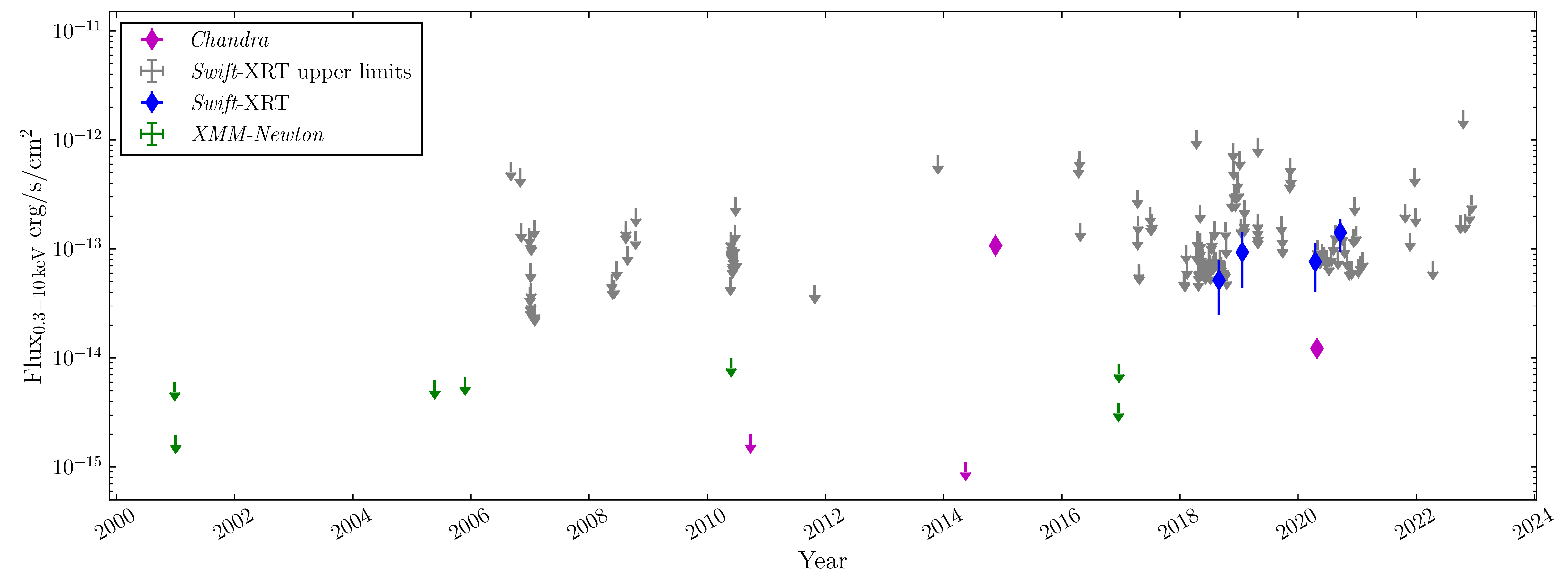
Figure 3: Long-term X-ray lightcurve of J0054. Magenta and green data refer to Chandra and XMM–Newton data, respectively; down-pointing arrows indicate $3\sigma$ upper limits while diamond markers indicate detections (with $1\sigma$ error bars). Swift/XRT detections are reported as blue diamonds, while the upper limits are indicated by down-pointing grey arrows. Count rates for the upper limits and for the Swift/XRT detections were converted to fluxes assuming the same spectral shape of the Chandra 2014 detection. Years are on the X-axis and flux in the 0.3–10 keV band is on the Y-axis.

2.4 Spectral fitting

Here we address the X-ray spectral fitting of J0054. In particular, we focus on its first detection with Chandra in November 2014, which is the data set with the highest count statistics.

The spectra, the spectral redistribution matrix and the ancillary response file were generated using the CIAO script specextract. The spectrum of J0054 was fed into the spectral fitting package XSPEC (Arnaud, 1996) version 12.12.1. Spectral channels having energies below 0.5 keV and above 7.0 keV were ignored in the fit, owing to the very low signal-to-noise ratio from J0054 (essentially all the counts are between approximately 0.7 and 1.7 keV). The spectra were grouped to have a minimum of 1 count per energy bin, and C-statistic (Cash, 1979) was employed (for the spectra shown in Fig. 4, further rebinning has been adopted for display purposes only).

We fit to the spectra a number of different simple models including (but not limited to) blackbody (bbody), power law, bremsstrahlung, Raymond–Smith plasma (Raymond & Smith, 1977), hot diffuse gas (MEKAL, Mewe et al. 1985, 1986; Liedahl et al. 1995), collisionally-ionized gas (APEC, Smith et al. 2001), and accretion disc model with multi-blackbody components (diskbb , with standard colour-correction factor fixed at 1.7, Lorenzin & Zampieri 2009) all corrected for interstellar absorption (TBabs, with $N_{\rm H}$ fixed to the Galactic value $9.45\times 10^{20}$ cm^-2; HI4PI Collaboration et al. 2016). The abundances used are those of Wilms et al. (2000), with the photoelectric absorption cross-sections from Verner et al. (1996).

While the power law, MEKAL, APEC, Raymond-Smith plasma and bremsstrahlung models provide unacceptable fits ($C/\nu$ between 2 and 3, $C$ being the value of the statistic and $\nu$ the number of degrees of freedom); both the bbody and diskbb can reproduce well the spectrum, and the fits improved when an extra-layer of absorption and an absorption Gaussian line at $1.13\pm 0.01$ keV with width fixed to 0 and normalization $K=(-1.4\pm 0.4)\times 10^{-5}$ photons cm^-2 s^-1, are added (EW$=0.077\pm 0.002$ keV). The significance of the extra layer of absorption and of the Gaussian line were tested with simulations. In both instances, the Xspec routine simftest returned a $<0.01\%$ probability that the data are consistent with the model without the extra component. Furthermore, the statistic improvement of adding the line is $\Delta C=35.1$ for three degrees of freedom: even accounting for the ”look elsewhere” effect (e.g., Lyons 2008), as the absorption feature does not line up with a specific atomic transition, by correcting the obtained p-value for the dimension of the energy space, i.e. multiplying it for the ratio between the bandwidth and the average resolution: $(2\leavevmode\nobreak\ {\rm keV}$–$0.5\leavevmode\nobreak\ {\rm keV})/0.05\leavevmode\nobreak\ \rm{keV}\approx 30$, the line significance results to be $>$$3.9\sigma$. For both models, the best-fit parameters are reported in Tab. 1.

Table 1: X-ray spectral fitting parameters.

model1	$N_{\textup{H}}^{2}$	$kT$	$K^{3}$	$M_{\textup{h}}^{4}$	$L_{\textup{X}}^{5}$	$C/\nu^{6}$	g.o.f.7
bbody	$0.73_{-0.13}^{+0.16}$	$0.109\pm 0.006$	$7.0_{-2.9}^{+6.6}\times 10^{-5}$	–	$1.9_{-0.8}^{+1.3}$	80/80	$26\%$
diskbb	$0.87_{-0.15}^{+0.14}$	$0.117_{-0.003}^{+0.009}$	$2.2_{-1.3}^{+3.8}\times 10^{3}$	1.0	$4.3_{-1.8}^{+1.6}$	79/80	$27\%$
slimd	$0.9\pm 0.1$	–	$0.11_{-0.01}^{+0.02}$	$1.4_{-0.4}^{+1.0}$	$3.6_{-0.9}^{+1.5}$	74/80	21%

Both the bbody and diskbb models provided similar temperatures, $kT\approx 110-120$ eV, and similar amounts of intrinsic absorption, $N_{\textup{H}}\approx(0.7$–$0.8)\times 10^{22}$ atoms cm^-2. The diskbb model naturally suggests a black hole (BH) as the accretor. From the fit we get an emitting region of $\approx$9000 km, which corresponds, under the assumption of Schwarzschild metric and $45^{\circ}$ disc inclination, to a mass of about $1000\,M_{\odot}$. This model also naturally suggests the presence of an accretion disc. Since J0054 is a transient source, to investigate better this possibility, we tried a model designed to reproduce accretion discs around black holes in transient events, slimd (Wen et al., 2022). As in the previous cases, we added to the slimd model the two layers of absorption (one fixed to the Galactic value, as above, and the other free to vary) and an absorption Gaussian line at 1.13 keV, and kept the disc inclination and spin fixed at $45^{\circ}$ and 0, respectively. We obtained good fit (Tab. 1) for a BH with mass $1.4_{-0.4}^{+1.0}\times 10^{3}\,M_{\odot}$ and moderate values of accretion rate ($\dot{m}=0.11_{-0.01}^{+0.02}\,\dot{m}_{\textup{Edd}}$, where $\dot{m}_{\textup{Edd}}$ indicates the maximum Eddington accretion rate) and intrinsic absorption $N_{\textup{H}}=0.9_{-0.1}^{+0.1}\times 10^{22}$ cm^-2, where errors correspond to a variation of the statistics $\Delta C=1$ (1$\sigma$). We note that both the BH mass and mass accretion rate heavily correlate with the intrinsic absorption, as shown by the contour plots in Fig. 5. The value of unabsorbed X-ray luminosity (between $0.3$ and $7$ keV), computed with this model and assuming J0054 is located in NGC 300, amounts to $3.6\times 10^{39}$ erg s^-1, which is in the regime of the ultraluminous X-ray sources (ULXs, e.g. Kaaret et al. 2017; Pinto & Walton 2023).

The value derived for the BH mass is affected not only by statistical uncertainties but also by systematic ones: we assumed fixed disc inclination and spin, and of course, the estimate is model dependent. Furthermore, the slimd model does not support BH masses lighter than $1000\,M_{\odot}$, thus preventing us from fully exploring the parameter space, as highlighted by Fig. 5. In order to have an idea of these uncertainties, first of all we performed fits with different BH spin and disc inclination values: prograde rotation ($a_{\bullet}=0.99$) and edge-on ($\theta=90\degr$) provided heavier masses, up to some $10^{4}\,M_{\odot}$, although the maximally-rotating case ($a_{\bullet}=0.99$) provided an unacceptable fit ($C/\nu>3$). Counter-rotation ($a_{\bullet}=-0.99$) and face-on ($\theta=0\degr$) configuration provided, instead, lighter masses, but the slimd model would not allow us to explore the mass regime below $1000\,M_{\odot}$. To explore the lighter mass regime we employed the slimbh model (Sadowski, 2011; Straub et al., 2011). This is designed to describe slim accretion disks around Eddington-limited stellar-mass ($\lesssim$100 $M_{\odot}$) BHs and has an upper limit for the BH mass of $1000\,M_{\odot}$, thus complementing the slimd model. The slimbh model with disc inclination fixed at $45^{\circ}$ provides an unacceptable fit ($C/\nu>3$) as the BH mass peaks at $1000\,M_{\odot}$. A face-on configuration provides an acceptable fit ($C/\nu=70/85$, $10\%$ goodness of fit, i.e. the percentage of cases, out of 10 000 spectra simulated based on the model, in which the test statistic was less than that of the data) with a BH mass of $\approx 800\,M_{\odot}$. Finally, we note that from the diskbb model, with the corrections by Lorenzin & Zampieri (2009), the mass can be estimated from 320 to 1000$\,M_{\odot}$ in a 90% range for the inclination (0$\degr$–85$\degr$). All in all, although we can poorly constrain the BH mass, as it ranges from $\sim$300 to $10^{4}\,M_{\odot}$, the spectral results consistently indicate an IMBH.

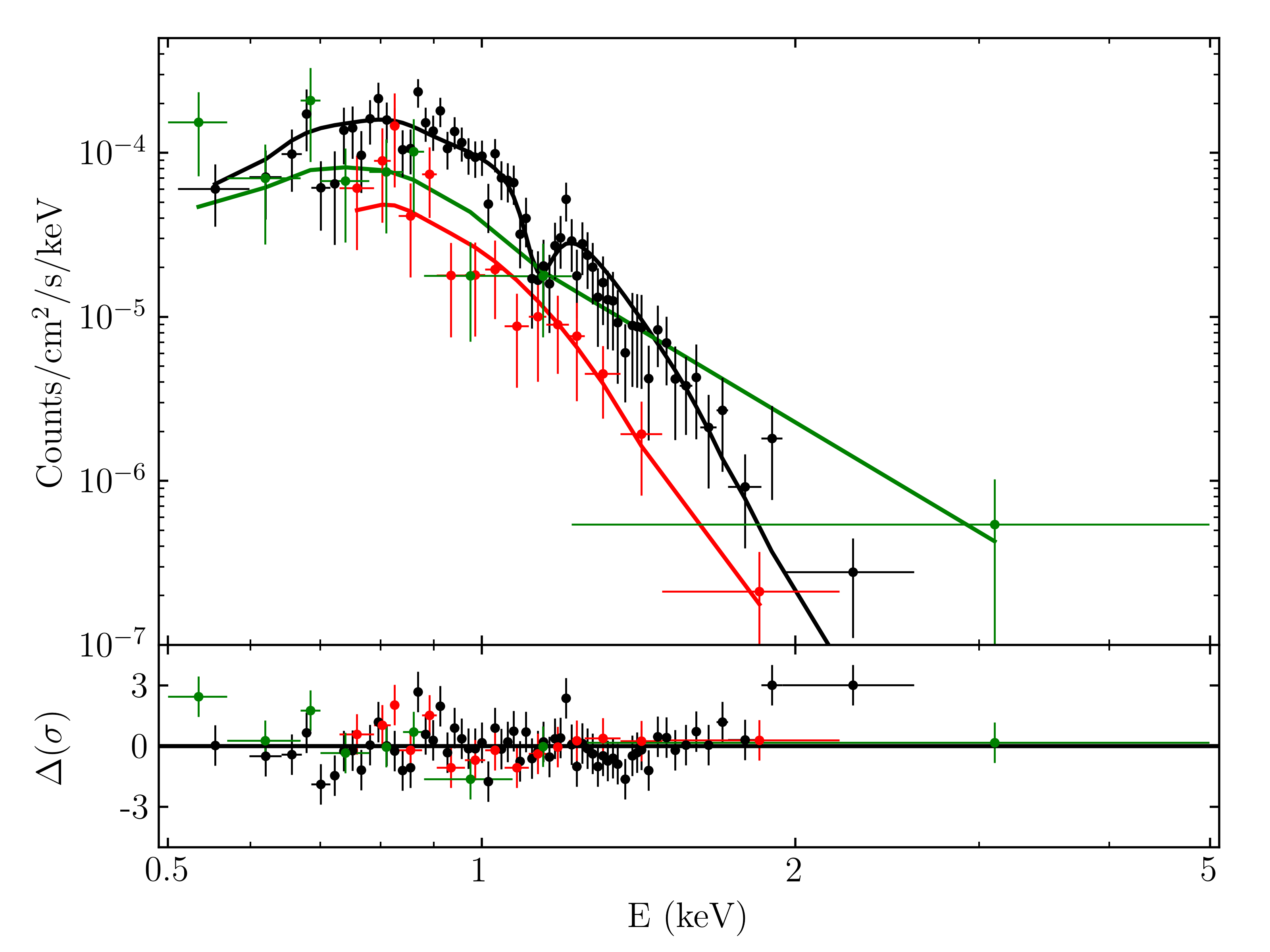
Figure 4: The upper panel shows the X-ray folded spectra and best-fitting model of J0054. Residuals are shown in the lower panel. Data from Chandra November 2014, April 2020 and Swift/XRT merged detections in black, red and green dots, respectively. Solid lines indicate the best-fitting slimd model.

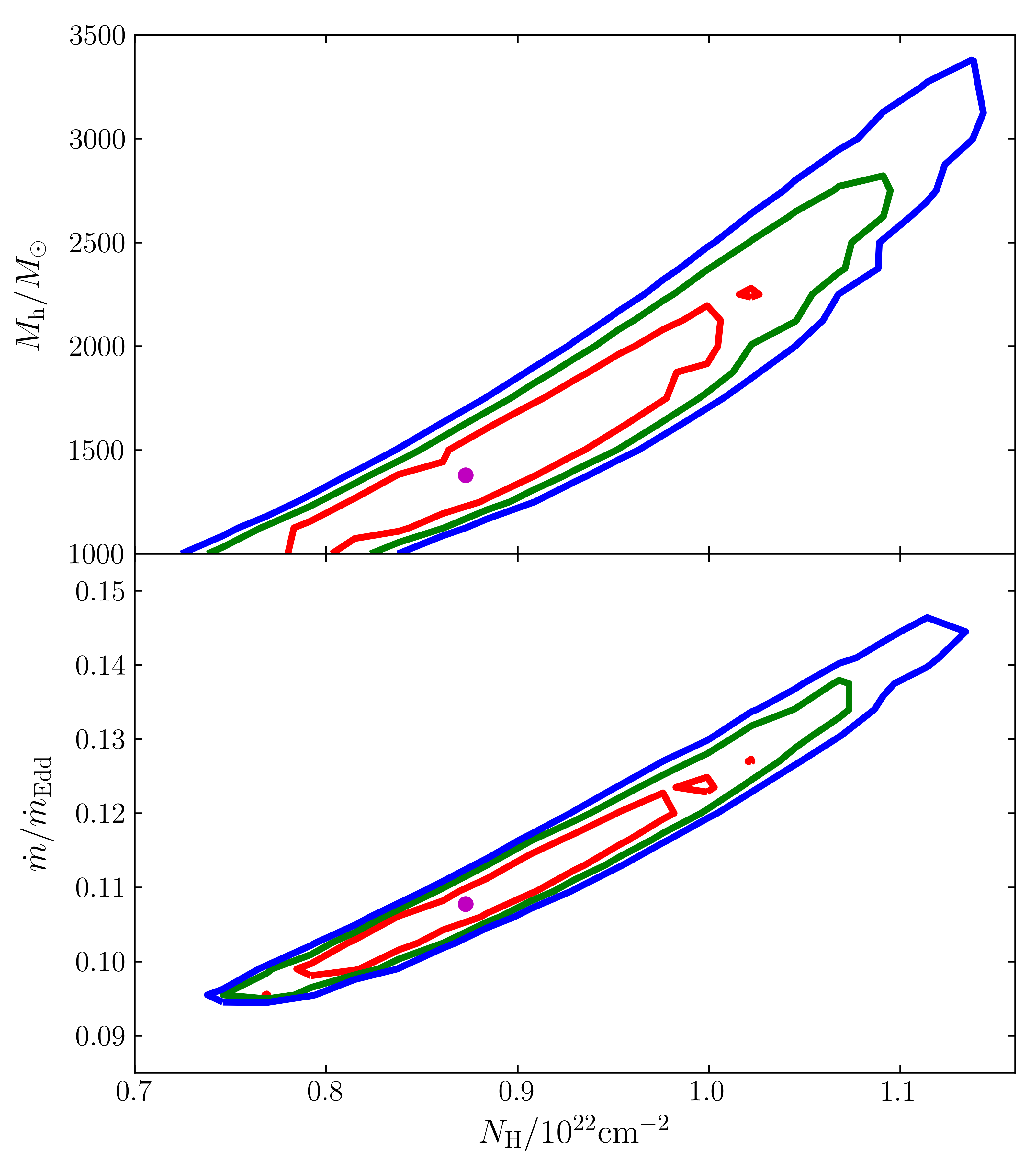
Figure 5: Contour plots in the BH mass–intrinsic absorption (upper panel) and mass accretion rate–intrinsic absorption spaces (lower panel) , obtained with the slimd model. Red green and blue contours indicate the $\Delta C=1,2,3$ levels, while the magenta dots are the best-fitting parameters.

Unfortunately, the spectra obtained in the other detections do not afford the possibility to perform meaningful spectroscopic analysis: the latest Chandra  detection, in April 2020, is heavily affected by the loss of effective area of the ACIS camera below $0.7$ keV, while the four Swift/XRT detections, taken individually, have too low signal-to-noise ratio for a spectrum to be extracted. Nonetheless, we tentatively merged data from all four Swift/XRT detections with the ftool routine extractor and extracted a merged spectrum with xselect from a circular region of 20 arcsec radius centred on the source position. The background was extracted from a free-of-sources circular region of 1 arcmin radius at a 3 arcmin distance from J0054 location and arfs likewise merged. In such a way, we reached a total of 32 net counts with a source fraction of the total counts evaluated at 94.3 %. We then fitted the best-fitting model we obtained above to the three spectra (the Chandra’s from November 2014 and April 2020, and the Swift/XRT one from the combined data sets) simultaneously. We froze all parameters to the best-fit ones, except for the normalizations (for the slimd model, it corresponds to the mass accretion rate). We obtained an acceptable value of the statistic ($C=119$ with 145 degrees of freedom and goodness of 31%) with no Gaussian lines in the latest Chandra observation and in the merged Swift/XRT spectra and mass accretion rates equal to $0.07$ and $0.09$ $\dot{m}_{\textup{Edd}}$ respectively. We can conclude that the emission of J0054 in the latest Chandra and in the Swift/XRT detections, is compatible with the one observed in the first Chandra detection, although spectral evolution or variations of the amount of intrinsic absorption cannot be assessed. Fig. 4 show the three spectra and their residuals in black, red and green, respectively, as well as the best-fitting model.

2.5 Optical/UV counterpart

2.5.1 UVOT photometry

As the location of J0054 was visited several times with Swift, we possess a large number of Swift/UVOT observations, which cover each of the 6 UVOT optical/UV bands: V (5468 Å), B (4392 Å), U (3465 Å), UVW1 (2600 Å), UVM2 (2246 Å), and UVW2 (1928 Å). Based on visual inspection, we removed any observations in which a smoke-ring feature, generated by the nearby foreground G8 star CD-38 301 (Cruzalèbes et al., 2019), was superimposed at the J0054 location.

We found no trace of significant variability (within $1\sigma$, roughly corresponding to half a magnitude) in any of the six bands; in particular, we found none in coincidence with the X-ray flaring activity, as shown in Fig. 6, which highlights the difference between the UVW2 AB magnitude and the 0.3–10 keV flux at the epoch of the latest flare. As no variability was detected, all observations were stacked using the ftool routine uvotimsum and fluxes were extracted using uvotsource (with flag APERCORR=curveofgrowth) from a circular region centred on the source position and with a radius of 5 arcsec. Backgrounds were estimated from a circular region of 10 arcsec radius, free of sources, at approximately 15 arcsec from the source location. The AB magnitudes from the merged Swift/UVOT observations are reported in Tab. 2, as well as the averaged magnitudes over the single observations.

In order to correct the Swift/UVOT spectral energy distribution (SED) for dust extinction we can adopt different strategies. The minimum possible value of the reddening is the Galactic line-of-sight value $E(B-V)=0.0108$ (Schlafly & Finkbeiner, 2011): in this case, the optical/UV SED would be consistent with a blackbody profile of $\approx$15,000 K and a luminosity of $7.5\times 10^{4}\,L_{\odot}$, compatible with a blue supergiant star ($M_{\rm V}\approx-6.5$ mag). A slightly higher reddening was adopted by Gieren et al. (2004), who assumed a foreground Galactic $E(B-V)=0.025$ mag (Burstein & Heiles, 1984) plus a reddening $E(B$–$V)=0.05$ mag through the halo of NGC 300. In this case, the best-fitting blackbody temperature rises to about 17,000 K and the luminosity to $10^{5}\leavevmode\nobreak\ L_{\odot}$, still compatible with a single blue supergiant star ($M_{\rm V}\approx-6.7$ mag).

However, the complete absence of individual stellar lines in the observed optical spectra (see Sec. 2.5.3) makes it unlikely that the observed SED stems from a barely reddened, single blue supergiant or a (very) late-type WR star with a comparable temperature (e.g. Sander et al., 2014).

The other extreme in terms of possible extinction would be to use the $N_{\rm H}$ inferred from the X-ray spectral modelling. Converted to an optical extinction $A_{\textup{V}}$ via the empirical relation in Foight et al. (2016), this would imply $A_{\rm V}\approx 3.1$ mag, and hence an absolute brightness $M_{\rm V}\approx-9.6$ mag. Such a source would be too luminous to be a single star and would further be unphysically blue ($B-V\approx-1.2$ mag) for any star, cluster, or blackbody-like spectrum. Thus, we can rule out such a high extinction for the optical counterpart. Assuming a physically meaningful limit of B$-$V $\gtrsim-0.5$ mag and $U-B\gtrsim-1.5$ mag, we can place an upper limit on the total extinction of $A_{\rm V}\lesssim 1$ mag. In this case, the photometry is compatible with a young stellar cluster (YSC) with an age of $\lesssim 4$ Myr and $\approx 10^{3}M_{\odot}$, assuming instantaneous star formation and a Large Magellanic Cloud (LMC)-like metallicity (similar to the one of NGC 300 : Gazak et al. 2015; Toribio San Cipriano et al. 2016). This would correspond to a small stellar population dominated by 3 or 4 main-sequence O stars and about $12-15$ B stars (see Sec. 2.5.3).

Table 2: UV/optical magnitudes from Swift/UVOT and XMM–Newton/OM.

Instrument	Epoch	AB Magnitude
		V	B	U	UVW1	UVM2	UVW2
Swift/UVOT (merged)	–	$19.84\pm 0.09$	$19.66\pm 0.05$	$19.75\pm 0.03$	$19.93\pm 0.04$	$20.06\pm 0.05$	$20.16\pm 0.05$
Swift/UVOT (averaged)	–	$19.82\pm 0.11$	$19.56\pm 0.09$	$19.77\pm 0.07$	$19.79\pm 0.07$	$19.85\pm 0.06$	$19.92\pm 0.05$
XMM–Newton/OM	2000-12-26	–	$20.2\pm 0.1$	–	–	–	–
	2001-01-01	–	$20.1\pm 0.1$	$20.3\pm 0.1$	$19.5\pm 0.1$	–	–
	2005-05-22	–	–	$20.0\pm 0.1$	$19.9\pm 0.1$	$20.2\pm 0.1$	–
	2005-11-25	–	–	$20.0\pm 0.1$	$19.62\pm 0.05$	$20.1\pm 0.1$	–
	2016-12-17	–	–	–	–	$20.3\pm 0.1$	–
	2016-12-19	–	–	–	–	$20.1\pm 0.1$	–

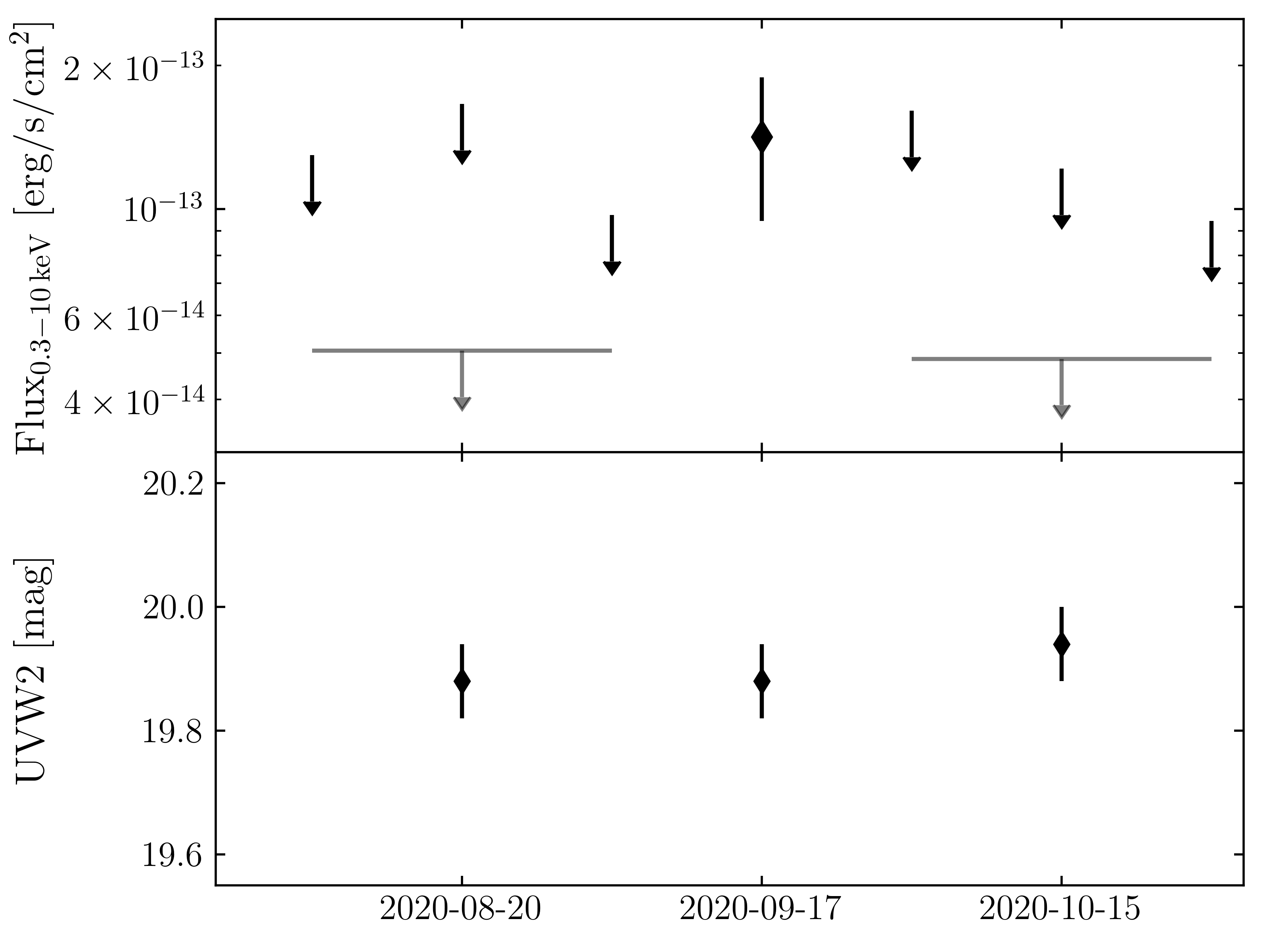
Figure 6: X-ray flux (upper panel) and UVW2 AB magnitude (lower panel) evolution during the flare detected in September 2020 Swift data. The X-ray upper limits in the single observations are reported as black arrows, the upper limits derived from the merged observations are reported as grey arrows. UVW2 magnitudes for each of the three epochs were derived by merging the single orbit exposures.

2.5.2 Archival data

J0054 is also present in the XMM–Newton/OM catalogue of serendipitous sources (Page et al., 2012). Our source location was visited six times as reported in Tab. 2. XMM–Newton/OM data are compatible with the Swift/UVOT ones when one considers that, at the magnitudes of our source, discrepancies as large as 1 magnitude are not uncommon between Swift/UVOT and XMM–Newton/OM (see Yershov 2014 and the XMM–Newton/OM calibration report). J0054 is also present in the Gaia catalogue (Gaia Collaboration et al., 2023), with a parallax $p=0.53\pm 0.78$ mas, corresponding to a distance of $1.2_{-0.4}^{+0.5}$ kpc (Lindegren et al., 2021; Bailer-Jones et al., 2021). However, at a magnitude $G=20.49$ ($G_{\textup{BP}}=20.61$ and $G_{\textup{RP}}=20.37$), the source is rather faint for Gaia and the low signal-to-noise ratio parallax is probably unreliable.

2.5.3 SALT spectrum

Two spectra were acquired on Dec. 2, 2019 and Dec. 15, 2019 (Progr.ID: 2018-2-LSP-001) with the Southern African Large Telescope (SALT) (Buckley et al., 2006; O’Donoghue et al., 2006), equipped with the Robert Stobie Spectrograph (RSS) (Burgh et al., 2003; Kobulnicky et al., 2003) in the long-slit ($8^{\prime}\times 1\aas@@fstack{\prime\prime}5$) spectroscopy mode. The PG0300 and PG0900 gratings were used for the observations with exposure times of 1800 s and 2000 s, respectively. A grating tilt of $5\aas@@fstack{\circ}4$ was used for the PG0300 observation, which covered the wavelength range 3700–7500 Å and provided a resolving power of 250–600. For the PG0900 observation, a tilt of $15\aas@@fstack{\circ}125$ (4200–7250 Å) was used, with a resultant resolving power of 800–1200. The position angle (PA) was 0 degrees from North and the average seeing during the observations was $1\aas@@fstack{\prime\prime}5$.

Standard spectral reduction (bias, flat-field, sky subtraction and cosmic-ray removal) was performed using PySALT pipeline (Crawford et al., 2010). The wavelength calibration was performed with the Ar (PG0300) and Xe (PG0900) lamps and the 1D spectrum was extracted using various tasks in IRAF. Since no spectrophotometric standard star was observed, the spectra are not calibrated in flux.

The two spectra show similar features and display strong emission lines of Balmer series and neutral He, as well as forbidden lines of [Oii], [Oiii], [Neiii], [Nii] and [Sii], with a blueward asymmetry, probably due to composite components in the emitting region, which however cannot be resolved with this resolution (see Fig. 7; the lower-resolution spectrum is shown in Fig. 11 and the parameters of the main lines, which were derived from Gaussian fits, are given in Tab. 4).

Figure 7: The SALT spectrum (PG0900) of J0054.

The lack of flux calibration does not allow us to measure emission line fluxes ratios. However, we can use the broadband SED from Swift/UVOT and the unabsorbed blackbody fit described in Sec. 2.5.1, to estimate an approximate continuum flux level (assuming that it did not change substantially between the Swift and SALT observations), and then convert the measured line equivalent width (EW) to line fluxes. In particular, we used the P0900 grating spectrum from 2019 December 15, which provides the more reliable measurement of the line profiles because of its higher resolution.

We find an observed flux ratio $F({\rm H}_{\alpha})/F({\rm H}_{\beta})\approx 2.9$ and $F({\rm H}_{\gamma})/F({\rm H}_{\beta})\approx 0.47$, perfectly consistent with photo-ionized gas in HII regions (Case B recombination) without any reddening corrections apart from the line-of-sight Galactic component. Our simulations with the starburst99 code (Leitherer et al., 1999, 2014) show that the EWs of H_α and H_β are consistent with those expected from photo-ionized gas illuminated by a YSC with the same continuum flux we observed. Both of those findings suggest that the emission lines are from an extended ionized nebula rather than from the direct stellar counterpart of the X-ray source. Moreover, the ionized gas sees the same continuum flux as we observe. If there is additional intrinsic extinction, it must be located between the X-ray source and the surrounding nebula, rather than between the source of the line emission and the line of sight.

We note that an O-type ionizing star embedded in a Hii region is not supported by the lack of absorption features of Heii and Hei (McLeod et al., 2015, 2020) while only Hei in emission is observed.

If the 6-hr periodicity identified in the X-ray lightcurve corresponds to the orbital period of a binary system, a compact, WR-like donor is needed: assuming a total mass of the system of $\approx 30\,M_{\odot}$ and a mass ratio of $\approx 3$, the binary separation amounts to $\approx 5\,R_{\odot}$ and the upper limit on the radius of the companion to $\approx 2.5\,R_{\odot}$. However, our SALT spectra do not show any explicit WR features, such as broad Heii 4686 Å emission (e.g. Dodorico et al. 1983). Also, the lack of a number of diagnostic lines (Schild & Testor, 1992) does not support a WC or a WN: Ciii, Cii, or Civ for the former and Niii 4100 Å and 4640 Å for the latter, are not detected. While this could in principle be explained by a compact (“stripped”) star that does not show WR-type spectral features (e.g. Götberg et al., 2018), such stars are a huge source of Heii ionizing flux (e.g. Sander & Vink, 2020; Sander et al., 2023), which should result in nebular Heii emission, which is absent as well. We thus ran starburst99 simulations to test whether stellar line emission features from a WR star could be hidden in a YSC with the observed continuum brightness and the line emission from its surrounding Hii region. Assuming the same uniform extinction $A_{\rm V}\approx 1$ mag for both the YSC and a WR star inside it, we verified that all features of a typical compact WR would be sufficiently diluted at least for some classes of WRs. For the WR, we used LMC models from Hainich et al. (2014) calculated with the PoWR (Gräfener et al., 2002; Hamann & Gräfener, 2003; Sander et al., 2015) model atmosphere code and diluted to the distance of NGC 300. From our calculations, we can thus conclude that the lack of observed WR emission lines in the SALT spectra does not rule out the scenario of a WR donor for the X-ray source. Moreover, an additional viable scenario is that the extinction around the X-ray binary system (including a WR donor with a dense wind) is higher than the extinction of the surrounding group of OB stars, which would further dilute or completely hide strong WR emission lines.

3 Discussion

J0054 is a puzzling source. It was discovered as a bright X-ray pulsator with a 6 h modulation, it shows a peculiar supersoft X-ray spectrum and displayed variability also on long-term. The available spectroscopy and photometry for the optical/UV counterpart show no hints of variability, but reveal only an HII region. While the photometry as such could match an individual B-star the strong absorption in the X-ray regime indicates that the photometry reflects an unresolved population of stars. Thus, any B-star, O-star, WR-star or even a whole YSC are viable options. In any case, the optical/UV and X-ray cannot be fitted simultaneously by a single black body or disk model, nor it is possible to intercept the optical/UV data extrapolating the model best-fitting the X-ray and vice versa (even accounting for the parameters’ uncertainties), as clearly demonstrated by Fig. 8, which shows the full SED and the absorbed and de-absorbed models. This suggests that the two emissions, optical/UV and X-ray, have different origins. Here we discuss different scenarios which could explain its peculiar multiwavelength appearance.

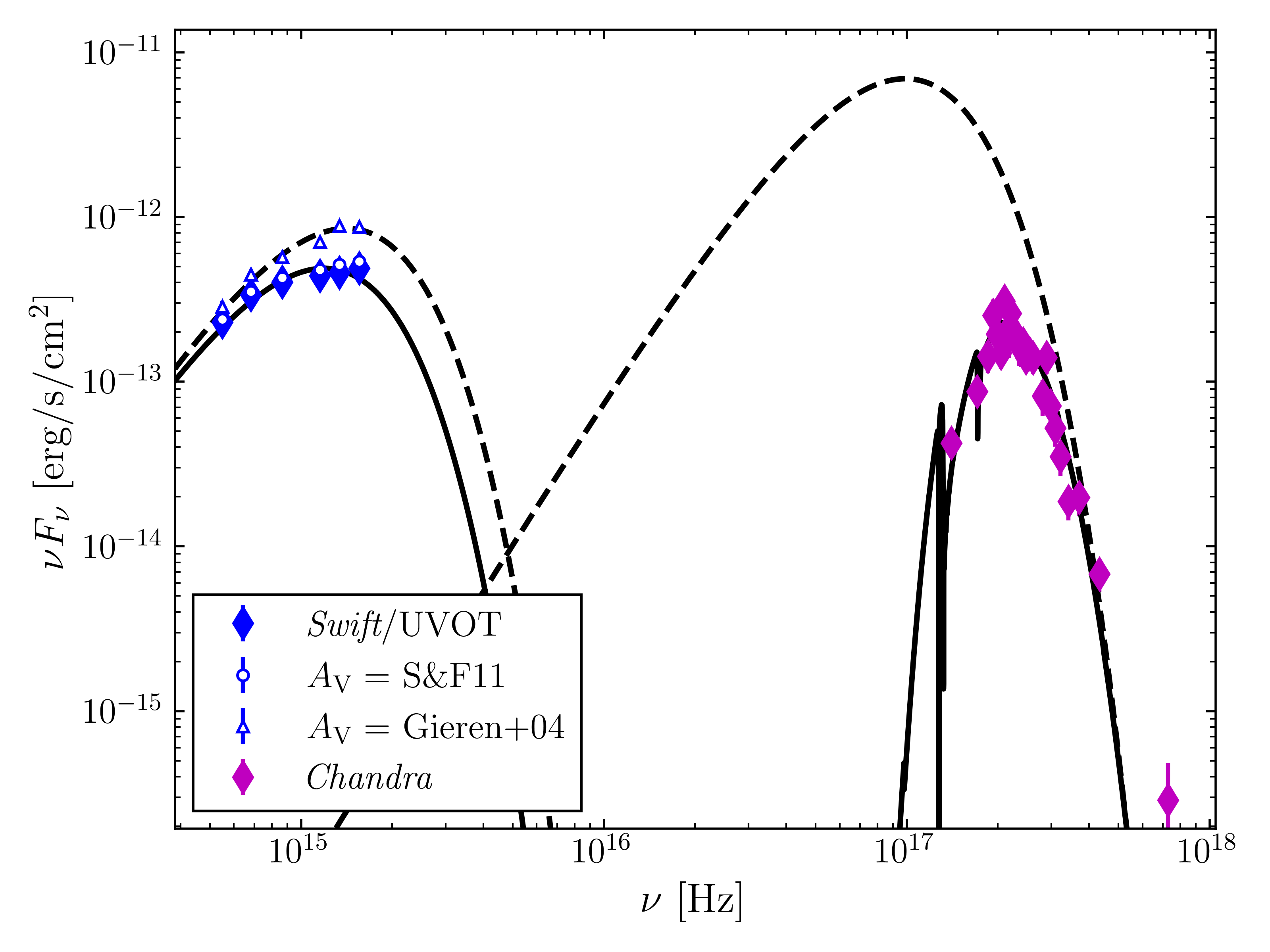
Figure 8: Full SED of J0054. Magenta and blue diamonds show the Chandra and Swift/UVOT data respectively. The black solid lines show the two independently best-fitting models for the two components with no absorption correction, and the dashed black lines show the de-absorbed models. For Swift/UVOT, the full markers indicate the observed flux, while the empty blue markers the de-absorbed fluxes, corrected following the different values discussed in the text (the full markers lie under the empty ones). For Chandra, de-absorbed model was obtained by putting to 0 the amount of $N_{\textup{H}}$.

Projected in the sky, J0054 is seen well inside the B-$R_{25}$ radius of NGC 300, at only 3.4 arcmin (about 1.9 kpc) from the center of the galaxy. Also, the Galactic latitude is $b\simeq-79\aas@@fstack{\circ}4$, making a Galactic foreground object highly unlikely. The only piece of information, possibly suggesting a foreground Galactic object, is the Gaia parallax, which is, however, probably unreliable given its low S/N. In the hypothesis of a Galactic object, in view of the 6 h modulation, the pulse profile and the flux, a cataclysmic variable (CV) is the only plausible candidate (although the X-ray spectrum discourages this interpretation and CVs are very unlikely to occur at the latitude of J0054; e.g. Drake et al. 2014). If the X-ray period traces the binary motion, for a CV in a 6-h orbit, a donor of spectral type of K7V (Knigge, 2006) is expected. If we assume for it $M_{\textup{V}}=7.7$, $B-V=1.3$, and $V-R=1.15$ (e.g. Johnson, 1966; Gray & Corbally, 2009), the possibility appears unlikely, since a late type K7V would be too bright and red with respect to our source optical counterpart. In the case of weakly-magnetic or non-magnetic system, the relationship between luminosity and orbital period by Warner (1987) indicates absolute magnitudes of $V\approx 4$ in a high state or $\approx$8 while in quiescence. More in general, the absolute magnitudes of such systems are always between 8 and 2 (Ramsay et al., 2017) and are therefore incompatible with the optical counterpart of J0054.

The lack of correlation between the X-ray flares and the optical/UV emission and the overall lack of significant variability at optical/UV wavelength across years does not support a nova at later stages (Williams et al., 1994; Williams, 2016) nor a super-soft source (SSS; van den Heuvel et al. 1992). A SSS scenario on the other hand is also discouraged by the fact that the observed X-ray and optical luminosity would require a massive WD, of about $1.2\,M_{\odot}$ (Starrfield et al., 2004) and this would place J0054 at $\approx 50$–200 kpc, which would result in an isolated intergalactic SSS, a highly unluckily occurrence.

The most natural way to explain the multi-wavelength behaviour of J0054 is probably an ultraluminous supersoft X-ray source (ULSs) scenario. ULSs can be considered as high-inclination, high-accretion rate compact objects. Here, the hard X-ray photons coming from the inner regions are significantly blocked by a strong optically-thick wind, which manifests itself in the form of Doppler-shifted absorption lines similar to the feature shown at 1.13 keV in Fig. 4  (Pinto & Walton, 2023; Urquhart & Soria, 2016). Moreover, this feature seems to be a hallmark strongly associated with the ULS population (Urquhart & Soria, 2016).

A well-known example is NGC 247 ULS or X–1 for which high-resolution spectra resolved the 1 keV feature into a forest of lines produced by a powerful $0.17c$ wind (Pinto et al., 2021); this source also exhibits modulations on timescales of a few ks (Alston et al., 2021). Here, the spectral-timing analysis would rather support the case for a heavy NS or a small stellar-mass BH accreting well beyond the Eddington limit (D’Aì et al., 2021).

J0054 also shares some spectral characteristics of M 101 ULX-1, a well-studied ULX and supersoft source consisting in a stellar-mass BH and a WR star (Liu et al., 2013). Indeed, the only object compatible with the 6 h modulation, if it reflects the binary orbit, is a WR (see Esposito et al. 2013a, 2015; Qiu et al. 2019 for the discussion of similar systems and candidates). As discussed in Sect. 2.5.3 a WR, isolated or belonging to a YSC, is not excluded by the optical information. While for the compact object, it is unsafe to rule out a neutron star only on the basis of the observed super-Eddington luminosity (e.g. Bachetti et al. 2014; Israel et al. 2017), a stellar-mass BH is the most likely compact object in WR binaries for evolutionary reasons (van den Heuvel et al., 2017). Both sources exhibit a highly variable (by a factor of $\approx$300) X-ray emission with a similar spectrum (at least in some states of M 101 ULX-1). In particular, similar temperature, size, and a dip at 1.1 keV (Soria & Kong, 2016; Urquhart & Soria, 2016).

Finally, it is worth mentioning that the NGC 300 galaxy hosts another bright source, a.k.a. NGC 300 X–1, which hosts a WR star feeding a massive black hole candidate (with a dynamically-inferred mass of $20\pm 4\,M_{\odot}$, although a lighter compact object cannot be completely ruled out; Laycock et al. 2015) which sometimes crosses the $10^{39}$ erg s^-1 threshold (Crowther et al., 2010; Earnshaw & Roberts, 2017).

The fact that the absorption inferred from the X-ray spectrum is local to the X-ray source and does not involve the optical counterpart (as demonstrated in Sect. 2.5.1) might support an outflowing wind in this scenario. However, the main problem with a ULX/ULS scenario is probably the transient nature of the source as, with a compact object in such a tight orbit with a strongly-winded WR, one would always expect significant accretion. A possible solution to this would be interpreting the variability in terms of obscuration, which would, however, likely result in spectral changes. The available data, unfortunately, are inconclusive about this matter. Finally we note that this source is not present in any ULX/ULS catalogues (e.g. Walton et al. 2022) because, although its unabsorbed luminosity exceeds the $10^{39}$ erg s^-1 threshold, its observed, absorbed luminosity does not.

A radically different scenario, which is capable of explaining some—although not all—features of J0054, is the partial tidal disruption of a star by an intermediate-mass BH (IMBH). Tidal disruption events (TDEs) occur when a star wanders too close to a supermassive BH (SMBH)—usually—and its binding self-gravity gets overcome by the BH’s tidal forces, tearing the star apart. Part of the stellar debris gets subsequently circularized and accreted, emitting a bright electromagnetic (EM) signal, and part gets ejected (Rees, 1988; Phinney, 1989). TDEs, although being bright across all EM spectrum, from radio to $\gamma$-rays (e.g Swift J1644, Burrows et al. 2011), in the X-ray band usually appear as luminous super-soft transients. Indeed, the X-ray spectrum suggests that J0054 emission is linked to accretion processes and the slimd model (specifically developed to fit slim disk emission from the tidal disruption of stellar objects by SMBHs) provides an estimate for the mass of J0054 ($\approx$1400 $M_{\odot}$) placing it in the IMBH class. The TDE hypothesis could also explain the observed long-term X-ray variability. As invoked for XMMU J122939.7+075333 (Tiengo et al., 2022), an object sharing with J0054 many characteristics (long-term variability, very soft X-ray emission, forbidden lines in the optical counterpart), a star on a highly eccentric orbit would get stripped of its material at every pericentre passage, thus producing recurrent flares.

Assuming we spotted the TDE close to its peak luminosity, we can use the mass accretion rate and BH mass obtained from the spectral fit to derive the penetration factor, orbital eccentricity and mass of the stripped star. To do so, we employed reasonable mass-radius relations for a white dwarf (WD) and for a main sequence star (MS), coupled with the analytical formulas derived by Guillochon & Ramirez-Ruiz (2013) for the $\gamma=5/3$ polytrope case. Fig. 9 shows the possible combination of star mass and orbital eccentricity compatible with the spectral estimates of mass accretion rate and BH mass. The blue and red contours represent the results obtained for a main sequence star and a white dwarf, respectively. The width of the contours corresponds to the $5\sigma$ region. The penetration factor $\beta$, defined as the ratio between pericentre distance and tidal radius, measures how deep the star dives into the potential well of the hole. As the tidal radius $r_{\textup{t}}\simeq r_{\star}(M_{\textup{h}}/m_{\star})^{1/3}$, represents the distance at which the BH tidal forces balance the stellar self-gravity, for penetration factors $\beta<1$ the disruption is only partial. For values of $\beta\lesssim 0.5$ the mass loss of the star stops (Guillochon & Ramirez-Ruiz, 2013): in Fig. 9 grey bars cover these forbidden regions. As Fig. 9 shows, only stars with masses below one solar mass are compatible with the spectral fitting results. Furthermore, for a WD only highly eccentric orbits are permitted, with $0.94\lesssim e\lesssim 0.96$, while for MS stars only values of eccentricities $\lesssim 0.7$ are permitted. In any case, for both WDs and MS stars, the passage around the BH is shallow: the dashed black line in Fig 9 represents the values for which the penetration factor is $\beta=0.6$. As for the case of XMMU J122939.7+075333, the amount of mass accreted at every passage is very little: about $5.5\times 10^{-10}$ $M_{\odot}$. As pointed out by Tiengo et al. (2022), with these low values of mass getting accreted per passage, one such event can last for very long times and indeed XMMU J122939.7+075333 has been active for more than two decades. Finally, although the available observations are sparse and often provide only shallow upper limits, the outbursts of J0054 seem to recur on a time scale of $\approx$5 months, which is the time interval between the two closest outbursts and cannot be ruled out by non-detections.

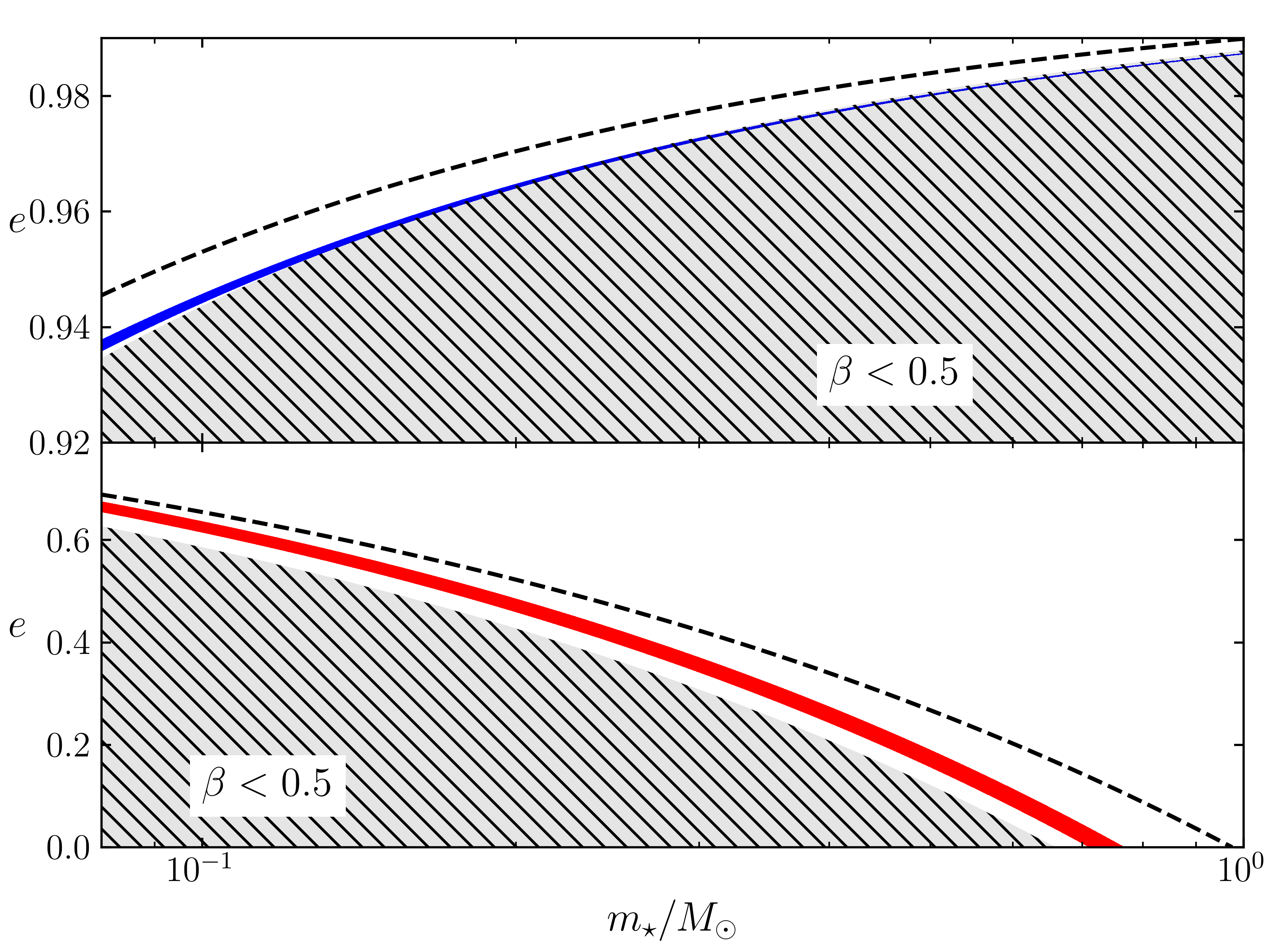
Figure 9: Orbital eccentricities and stellar mass values compatible with the BH mass and mass accretion rate obtained from the spectral fitting. Blue and red regions indicate WD and MS star cases respectively. The width of the contours covers the $5\sigma$ regions. The barred portions of parameter space are forbidden as they represent the regions where $\beta<0.5$ (no disruption occurs) and the dashed lines indicate the values for which $\beta=0.6$.

The TDE scenario could also explain J0054 short-term variability: the observed periodicity could be linked to disc instability in a similar way to the one described by Pasham et al. (2019) for the “text-book TDE” ASASSN-14li (Miller et al., 2015). To investigate this possibility, we can study the fundamental frequencies at the innermost stable circular orbit (ISCO) around the BH. These are three: the Keplerian orbital frequency $\nu_{\phi}$, the vertical epicyclic frequency $\nu_{\theta}$, and the Lense–Thirring one, given by the beating between these two, $\nu_{\textup{LT}}=\nu_{\phi}-\nu_{\theta}$. Analytical expressions for these frequencies were derived by Kato (1990):

$$\nu_{\phi}=\frac{c^{3}}{2\pi GM_{\textup{h}}}\left[\frac{1}{R_{\textup{ISCO}}^{3/2}+a_{\bullet}}\right],$$ (1)

$$\nu_{\theta}=\nu_{\phi}\left[1-\frac{4a_{\bullet}}{R_{\textup{ISCO}}^{3/2}}+\frac{3a^{2}_{\bullet}}{R_{\textup{ISCO}}^{2}}\right]^{1/2}.$$ (2)

Fig. 10 shows the contours, in the BH mass-spin space, for the three described frequencies, Keplerian (in red), vertical epicyclic (in green) and Lense–Thirring (in blue) for a $47\pm 1$ $\mu$Hz frequency (the $5.88\pm 0.12$ h modulation). The width of the contours represents the $5\sigma$ region. The shaded region shows the BH mass range identified by the spectral fit, its width corresponds to a $\Delta C=1$. The only frequency compatible with the mass range identified by the spectral fitting is the Lense–Thirring one and only for a non-spinning BH: $|a_{\bullet}|\lesssim 4\times 10^{-4}$.

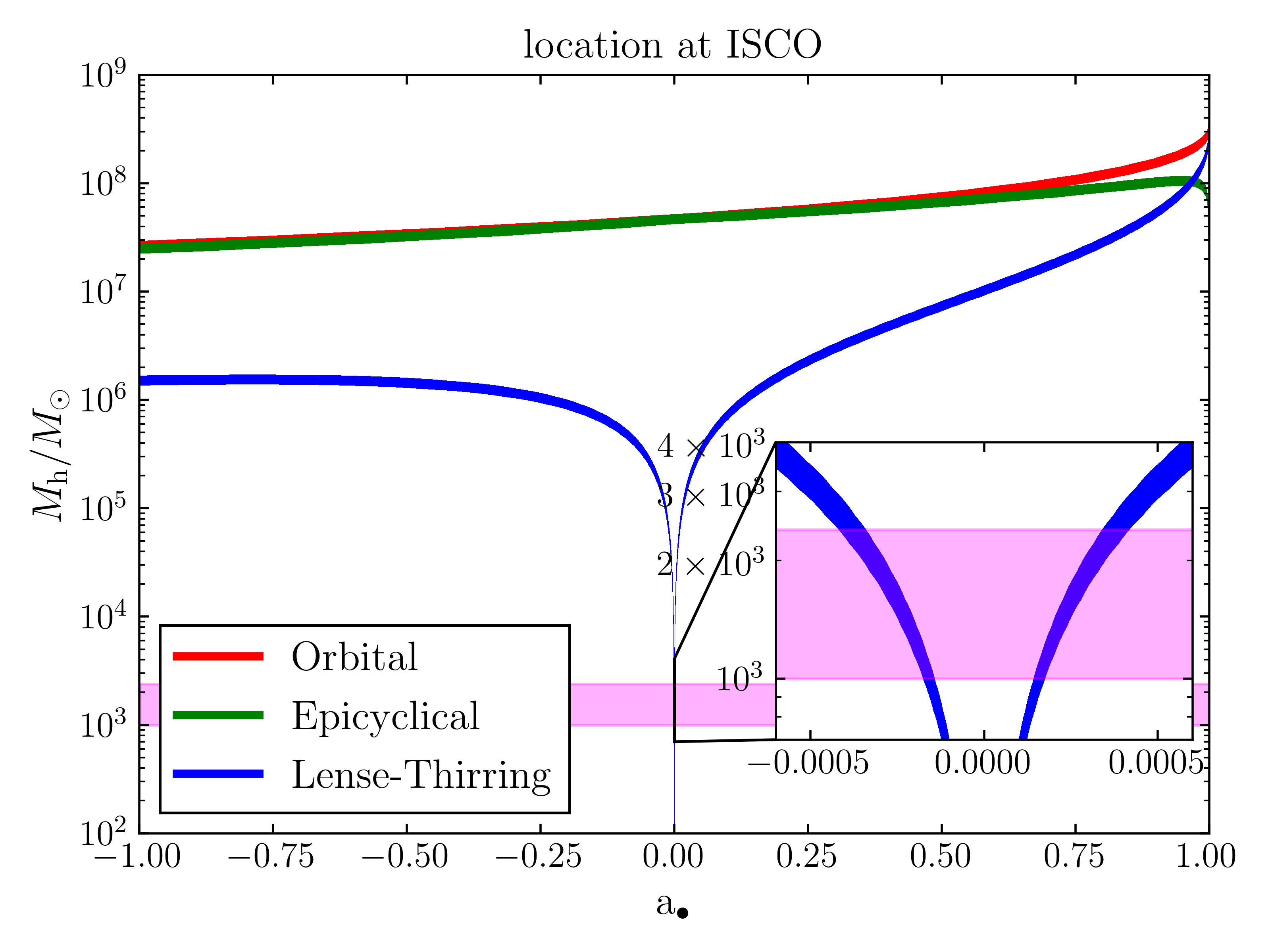
Figure 10: Contour plot in the BH mass-spin space of the three fundamental frequencies at ISCO for a 47 $\mu$Hz frequency. The shaded region indicates the BH mass range obtained from the spectral fit. The width of the lines reflects a $5\sigma$ range.

The TDE scenario cannot account for every aspect of J0054. The absorption feature in the X-ray spectrum, around 1 keV is similar to ones often observed in super soft sources, both Galactic (nuclear burning WD, see e.g. Ebisawa et al. 2001) and extragalactic (ULXs, see e.g. Pinto et al. 2021), however, this feature is usually detected in sources with thick outflows rather than simple disc emission, and only at high values of mass accretion rates. Another weak point in this scenario is the involvement of a non-spinning $10^{3}\,M_{\odot}$ IMBH. Albeit it has been shown that young dense clusters can nurture the seeding of IMBHs (Arca Sedda et al. 2021; Di Carlo et al. 2021; Rizzuto et al. 2021, 2022; Gonzalez et al. 2023; Arca Sedda et al., in prep), it seems hard for YSCs to grow IMBHs above 1000 $M_{\odot}$, unless the host YSC has large central densities (e.g. Maliszewski et al., 2022) and the tightly constrained null value of the spin would require some fine tuning for the model to work. On the other hand, the TDE scenario can provide a satisfactory explanation for the X-ray spectral shape and both the long- and short-term behaviour of J0054.

Appendix A X-ray observations

The journal of the X-ray observations is given in Tab. LABEL:tab:cxo. 1]

Table 3: Journal of the Chandra, XMM–Newton and Swift/XRT observations used in this work. Errors are at $1\sigma$ and upper limits at $3\sigma$. The corresponding fluxes are shown in Fig. 3.

Instrument	Obs.ID	Date	Exposure	Rate
			(ks)	(counts s-1)
XMM–Newton(pn)	0112800201	2000-12-26/27	30.0	$<2.64\times 10^{-3}$
XMM–Newton(pn)	0112800101	2001-01-01/02	40.0	$<8.73\times 10^{-4}$
XMM–Newton(pn)	0305860401	2005-05-22	28.1	$<2.76\times 10^{-3}$
XMM–Newton(MOS)	0305860301	2005-11-25	36.0	$<7.23\times 10^{-4}$
XRT	00035866001	2006-09-05	0.8	$<2.27\times 10^{-2}$
XRT	00035866002	2006-11-01	0.6	$<1.98\times 10^{-2}$
XRT	00035866003	2006-11-07	1.8	$<6.19\times 10^{-3}$
XRT	00030848001	2006-12-27	2.0	$<5.58\times 10^{-3}$
XRT	00030848002	2006-12-29	9.9	$<1.05\times 10^{-3}$
XRT	00030848003	2006-12-30	9.6	$<1.07\times 10^{-3}$
XRT	00030848004	2006-12-31	9.4	$<1.13\times 10^{-3}$
XRT	00030848005	2007-01-01	9.2	$<1.60\times 10^{-3}$
XRT	00030848006	2007-01-02	7.7	$<1.33\times 10^{-3}$
XRT	00030848007	2007-01-03	8.8	$<1.21\times 10^{-3}$
XRT	00030848008	2007-01-04	2.3	$<4.90\times 10^{-3}$
XRT	00030848009	2007-01-05	5.0	$<2.65\times 10^{-3}$
XRT	00030848010	2007-01-06	8.7	$<1.37\times 10^{-3}$
XRT	00030848011	2007-01-07	7.0	$<1.76\times 10^{-3}$
XRT	00030848012	2007-01-08	3.8	$<4.67\times 10^{-3}$
XRT	00035866004	2007-01-28/29	1.7	$<6.65\times 10^{-3}$
XRT	00031210001	2008-05-20	6.1	$<2.14\times 10^{-3}$
XRT	00031210002	2008-05-25	7.1	$<1.85\times 10^{-3}$
XRT	00031210003	2008-06-04	6.9	$<1.88\times 10^{-3}$
XRT	00031210004	2008-06-19	8.0	$<2.77\times 10^{-3}$
XRT	00031210005	2008-08-14	2.1	$<6.52\times 10^{-3}$
XRT	00031210006	2008-08-15	2.2	$<6.00\times 10^{-3}$
XRT	00031210007	2008-08-26	4.7	$<3.97\times 10^{-3}$
XRT	00031210008	2008-10-15	2.1	$<5.28\times 10^{-3}$
XRT	00031210009	2008-10-16	1.6	$<8.56\times 10^{-3}$
XRT	00031726001	2010-05-24/26	6.6	$<2.01\times 10^{-3}$
XRT	00031726002	2010-05-26	2.7	$<5.19\times 10^{-3}$
XMM–Newton(pn)	0656780401	2010-05-28	18.1	$<4.42\times 10^{-3}$
XRT	00031726003	2010-05-28	3.2	$<4.27\times 10^{-3}$
XRT	00031726004	2010-05-30	3.2	$<4.02\times 10^{-3}$
XRT	00031726005	2010-06-01	3.9	$<4.68\times 10^{-3}$
XRT	00031726006	2010-06-03	3.0	$<4.38\times 10^{-3}$
XRT	00031726007	2010-06-05	4.5	$<2.89\times 10^{-3}$
XRT	00031726008	2010-06-07	4.1	$<3.16\times 10^{-3}$
XRT	00031726009	2010-06-09	4.0	$<3.28\times 10^{-3}$
XRT	00031726010	2010-06-11	3.8	$<3.57\times 10^{-3}$
XRT	00031726011	2010-06-16	4.0	$<4.49\times 10^{-3}$
XRT	00031726012	2010-06-17	4.2	$<3.19\times 10^{-3}$
XRT	00031726013	2010-06-18	4.2	$<3.23\times 10^{-3}$
XRT	00031726015	2010-06-21	2.2	$<6.01\times 10^{-3}$
XRT	00031726016	2010-06-25	1.3	$<1.07\times 10^{-2}$
XRT	00031726017	2010-07-01	4.0	$<3.36\times 10^{-3}$
Chandra	12238	2010-09-24/25	63.0	$<1.7\times 10^{-4}$
XRT	00031726018	2010-09-26	2.3	$<7.93\times 10^{-3}$
XRT	00031726019	2010-09-27	3.5	$<3.76\times 10^{-3}$
XRT	00031726020	2010-09-28	4.3	$<3.08\times 10^{-3}$
XRT	00049834001	2013-11-27	0.5	$<2.6\times 10^{-2}$
Chandra	16028	2014-05-16/17	64.2	$<9.3\times 10^{-5}$
Chandra	16029	2014-11-17/18	61.3	$(9.0\pm 0.4)\times 10^{-3}$
XRT	00049834002	2016-04-14	0.6	$<2.38\times 10^{-2}$
XRT	00049834003	2016-04-20	0.5	$<2.83\times 10^{-2}$
XRT	00049834005	2016-04-24/25	2.9	$<6.28\times 10^{-3}$
XMM–Newton(pn)	0791010101	2016-12-17/18	102.6	$<1.72\times 10^{-3}$
XMM–Newton(pn)	0791010301	2016-12-19/20	47.5	$<3.90\times 10^{-3}$
XRT	00049834006	2017-04-13	1.1	$<1.26\times 10^{-2}$
XRT	00049834007	2017-04-14/15	2.5	$<5.23\times 10^{-3}$
XRT	00049834008	2017-04-16/7	1.9	$<7.25\times 10^{-3}$
XRT	00049834009	2017-04-21	0.5	$<2.63\times 10^{-2}$
XRT	00049834010	2017-04-24	5.2	$<2.51\times 10^{-3}$
XRT	00049834012	2017-07-02	1.3	$<8.76\times 10^{-3}$
XRT	00049834013	2017-07-06	1.9	$<7.02\times 10^{-3}$
XRT	00049834014	2017-07-12	1.8	$<7.48\times 10^{-3}$
XRT	00049834015	2018-01-25	5.0	$<2.25\times 10^{-3}$
XRT	00088651001	2018-01-31	5.1	$<2.17\times 10^{-3}$
XRT	00049834016	2018-02-07	4.6	$<3.91\times 10^{-3}$
XRT	00049834017	2018-02-14	4.8	$<2.83\times 10^{-3}$
XRT	00049834018	2018-04-12	0.3	$<4.42\times 10^{-2}$
XRT	00049834019	2018-04-13/14	3.5	$<3.87\times 10^{-3}$
XRT	00049834020	2018-04-18	2.6	$<5.22\times 10^{-3}$
XRT	00049834021	2018-04-25	6.1	$<2.19\times 10^{-3}$
XRT	00049834022	2018-04-26	5.2	$<2.55\times 10^{-3}$
XRT	00049834023	2018-04-27	4.9	$<3.70\times 10^{-3}$
XRT	00049834024	2018-04-28	4.8	$<2.75\times 10^{-3}$
XRT	00049834025	2018-04-29	4.9	$<3.66\times 10^{-3}$
XRT	00049834026	2018-04-30	5.0	$<2.70\times 10^{-3}$
XRT	00049834027	2018-05-01	4.7	$<3.71\times 10^{-3}$
XRT	00049834028	2018-05-02	5.0	$<3.58\times 10^{-3}$
XRT	00049834029	2018-05-03	4.9	$<2.83\times 10^{-3}$
XRT	00049834030	2018-05-04	4.8	$<2.71\times 10^{-3}$
XRT	00049834031	2018-05-05	1.5	$<9.21\times 10^{-3}$
XRT	00049834032	2018-05-06	4.5	$<5.00\times 10^{-3}$
XRT	00049834033	2018-05-07	3.2	$<4.25\times 10^{-3}$
XRT	00049834034	2018-05-08	6.2	$<3.52\times 10^{-3}$
XRT	00049834035	2018-05-11	4.9	$<3.72\times 10^{-3}$
XRT	00049834036	2018-05-14	4.9	$<2.78\times 10^{-3}$
XRT	00049834037	2018-05-17	4.8	$<2.76\times 10^{-3}$
XRT	00049834038	2018-05-20	4.7	$<2.95\times 10^{-3}$
XRT	00049834039	2018-05-23	4.9	$<3.58\times 10^{-3}$
XRT	00049834040	2018-05-26	4.8	$<2.80\times 10^{-3}$
XRT	00049834041	2018-05-29	4.7	$<2.79\times 10^{-3}$
XRT	00049834043	2018-06-01	4.9	$<2.80\times 10^{-3}$
XRT	00049834044	2018-06-07	5.2	$<2.55\times 10^{-3}$
XRT	00049834045	2018-06-10	4.7	$<2.86\times 10^{-3}$
XRT	00049834046	2018-06-13	4.9	$<2.68\times 10^{-3}$
XRT	00049834047	2018-06-16	4.7	$<2.87\times 10^{-3}$
XRT	00049834048	2018-06-19	4.7	$<2.85\times 10^{-3}$
XRT	00049834049	2018-06-28	3.8	$<3.60\times 10^{-3}$
XRT	00049834050	2018-07-03	4.3	$<3.20\times 10^{-3}$
XRT	00049834051	2018-07-08	4.4	$<2.53\times 10^{-3}$
XRT	00049834052	2018-07-13	3.7	$<4.83\times 10^{-3}$
XRT	00049834053	2018-07-18	3.6	$<5.12\times 10^{-3}$
XRT	00049834054	2018-07-23	4.3	$<3.09\times 10^{-3}$
XRT	00049834055	2018-07-28	3.8	$<3.64\times 10^{-3}$
XRT	00049834056	2018-08-02	3.9	$<3.45\times 10^{-3}$
XRT	00049834057	2018-08-07	4.0	$<3.38\times 10^{-3}$
XRT	00049834058	2018-08-12	4.0	$<3.38\times 10^{-3}$
XRT	00049834059	2018-08-29	3.6	$(1.9\pm 1.0)\times 10^{-3}$
XRT	00049834060	2018-09-05	3.8	$<3.52\times 10^{-3}$
XRT	00049834061	2018-09-12	4.5	$<3.02\times 10^{-3}$
XRT	00049834063	2018-09-23	4.8	$<2.73\times 10^{-3}$
XRT	00049834064	2018-09-26	4.6	$<2.87\times 10^{-3}$
XRT	00049834065	2018-10-03	4.7	$<2.76\times 10^{-3}$
XRT	00088810002	2018-10-07	4.9	$<2.66\times 10^{-3}$
XRT	00049834066	2018-10-10	2.1	$<6.39\times 10^{-3}$
XRT	00049834067	2018-10-14	2.9	$<4.40\times 10^{-3}$
XRT	00049834068	2018-10-17	4.7	$<2.27\times 10^{-3}$
XRT	00049834070	2018-11-18	1.0	$<1.17\times 10^{-2}$
XRT	00049834071	2018-11-25	0.4	$<3.41\times 10^{-2}$
XRT	00049834072	2018-11-28	0.6	$<2.31\times 10^{-2}$
XRT	00049834073	2018-12-02	1.0	$<1.43\times 10^{-2}$
XRT	00049834074	2018-12-09	1.1	$<1.18\times 10^{-2}$
XRT	00049834075	2018-12-16	1.0	$<1.41\times 10^{-2}$
XRT	00049834076	2018-12-23	0.6	$<1.79\times 10^{-2}$
XRT	00049834077	2018-12-30	0.9	$<1.46\times 10^{-2}$
XRT	00049834078	2019-01-06	0.3	$<4.21\times 10^{-2}$
XRT	00049834080	2019-01-13	2.0	$<6.83\times 10^{-3}$
XRT	00049834081	2019-01-20	2.0	$(3.4\pm 1.8)\times 10^{-3}$
XRT	00049834082	2019-01-27	1.8	$<1.02\times 10^{-2}$
XRT	00049834083	2019-02-03	1.8	$<7.68\times 10^{-3}$
XRT	00049834084	2019-02-10	2.0	$<6.95\times 10^{-3}$
XRT	00049834085	2019-04-13	2.1	$<6.56\times 10^{-3}$
XRT	00049834086	2019-04-20	2.5	$<5.37\times 10^{-3}$
XRT	00049834087	2019-04-27	0.4	$<3.73\times 10^{-2}$
XRT	00049834088	2019-05-04	2.3	$<5.81\times 10^{-3}$
XRT	00049834089	2019-05-11	2.1	$<7.56\times 10^{-3}$
XRT	00031726021	2019-09-20	1.9	$<7.16\times 10^{-3}$
XRT	00012017001	2019-09-26	2.5	$<5.45\times 10^{-3}$
XRT	00012017002	2019-09-26	3.0	$<4.48\times 10^{-3}$
XRT	00012017004	2019-09-27	3.1	$<4.43\times 10^{-3}$
XRT	00012160001	2019-11-11	0.8	$<1.75\times 10^{-2}$
XRT	00012160002	2019-11-14	0.8	$<2.49\times 10^{-2}$
XRT	00012160003	2019-11-16	1.2	$<1.94\times 10^{-2}$
XRT	00095672001	2020-04-16	3.7	$(2.8\pm 1.3)\times 10^{-3}$
Chandra	22375	2020-04-26/27	47.4	$(1.0\pm 0.2)\times 10^{-3}$
XRT	00095672002	2020-04-30	3.1	$<4.36\times 10^{-3}$
XRT	00095672003	2020-05-14	3.8	$<3.52\times 10^{-3}$
XRT	00095672004	2020-05-28	3.3	$<4.01\times 10^{-3}$
XRT	00095672005	2020-06-11	3.6	$<3.73\times 10^{-3}$
XRT	00095672006	2020-06-25	3.3	$<3.53\times 10^{-3}$
XRT	00095672007	2020-07-09	3.7	$<3.06\times 10^{-3}$
XRT	00095672008	2020-07-23	3.8	$<3.71\times 10^{-3}$
XRT	00095672009	2020-08-06	2.9	$<4.67\times 10^{-3}$
XRT	00095672010	2020-08-20	3.1	$<5.98\times 10^{-3}$
XRT	00095672011	2020-09-03	3.8	$<3.50\times 10^{-3}$
XRT	00095672012	2020-09-17	3.9	$(5.1\pm 1.7)\times 10^{-3}$
XRT	00095672013	2020-10-01	3.2	$<5.79\times 10^{-3}$
XRT	00095672014	2020-10-15	3.1	$<4.38\times 10^{-3}$
XRT	00095672015	2020-10-29	3.9	$<3.40\times 10^{-3}$
XRT	00095672016	2020-11-12	3.9	$<2.79\times 10^{-3}$
XRT	00095672017	2020-11-26	3.9	$<2.81\times 10^{-3}$
XRT	00095672018	2020-12-10	2.3	$<5.54\times 10^{-3}$
XRT	00095672019	2020-12-15	1.6	$<1.08\times 10^{-2}$
XRT	00095672020	2020-12-24	3.8	$<5.87\times 10^{-3}$
XRT	00095672021	2021-01-07	3.7	$<2.92\times 10^{-3}$
XRT	00095672022	2021-01-21	3.5	$<3.14\times 10^{-3}$
XRT	00095672023	2021-02-04	3.9	$<3.38\times 10^{-3}$
XRT	00031726022	2021-10-23	1.4	$<9.29\times 10^{-3}$
XRT	00031726023	2021-11-23	2.1	$<5.11\times 10^{-3}$
XRT	00031726024	2021-12-22	0.7	$<1.99\times 10^{-2}$
XRT	00031726025	2021-12-28	1.8	$<8.58\times 10^{-3}$
XRT	00031726028	2022-04-13	4.7	$<2.78\times 10^{-3}$
XRT	00031726029	2022-10-01	2.1	$<7.43\times 10^{-3}$
XRT	00031726030	2022-10-18	0.2	$<6.80\times 10^{-2}$
XRT	00031726031	2022-10-29	1.5	$<7.51\times 10^{-3}$
XRT	00031726033	2022-11-26	1.5	$<8.98\times 10^{-3}$
XRT	00031726034	2022-12-10	1.6	$<1.13\times 10^{-2}$

Table 3: Continued.

Appendix B SALT spectrum

The parameters of the emission lines in the optical SALT spectrum are reported in Tab. 4. The lower-resolution spectrum (PG0300) is shown in Fig. 11.

Figure 11: The SALT spectrum (PG0300) of J0054. Note that the lines labelled with a question mark are better identified and resolved in the PG0900 spectrum (Fig. 7).

Table 4: Parameters of emission lines in the two SALT spectra.

Element	$\lambda^{1}$	FWHM	EQW	V${}_{\textup{rad}}^{2}$	Notes
	(Å)	(Å)	(Å)	(km/s)
02 December 2019
[Oii]	$3729.1\pm 0.2$	$17.4\pm 0.5$	$332\pm 13$	$121\pm 17$	blend of $3726-3729\,\AA$
[Neiii]	$3872.3\pm 0.1$	$12.1\pm 3.7$	$9.7\pm 3.7$	$252\pm 12$	blended with Hei $3888.64\,\AA$
Hei	$3891.3\pm 0.9$	$14.0\pm 2.2$	$21.9\pm 4.1$	$182\pm 66$	blended with [Neiii] $3868.75\,\AA$
[Oiii]	$3960.0\pm 1.6$	$11.7\pm 3.8$	$12.6\pm 6.0$	$-143\pm 12$	uncertain identification
Hϵ	$3976.8\pm 1.1$	$13.7\pm 2.7$	$24.0\pm 8.2$	$483\pm 83$	blended possibly with [Oiii] $3961.59\,\AA$
Hδ	$4105.8\pm 0.6$	$16.6\pm 1.5$	$39.5\pm 4.8$	$275\pm 47$
Hγ	$4344.8\pm 0.3$	$17.1\pm 0.6$	$99.6\pm 4.9$	$273\pm 18$
Hei	$4477.03\pm 0.01$	$36.74\pm 0.01$	$5.0\pm 2.0$	$349.37\pm 0.01$	double peaked, manually measured
Hβ	$4867.0\pm 0.3$	$16.7\pm 0.7$	$330\pm 17$	$328\pm 16$	with additional red-component
[Oiii]	$4965.5\pm 0.3$	$15.2\pm 0.8$	$240\pm 18$	$375\pm 19$
[Oiii]	$5013.3\pm 0.3$	$16.0\pm 0.9$	$702\pm 51$	$365\pm 20$
Hei	$5883.4\pm 0.6$	$13.6\pm 1.4$	$113\pm 15$	$376\pm 2$9
Hα	$6569.7\pm 0.3$	$17.5\pm 0.7$	$1731\pm 89$	$294\pm 12$	blended with [Nii] $6548\,\AA$, and partially with $6584\,\AA$
[Nii]	$6593.4\pm 0.2$	$16.1\pm 0.6$	$8.6\pm 3.9$	$426.9\pm 7.3$	blended with Hα
[Sii]	$6726.0\pm 0.3$	$20.5\pm 0.8$	$288\pm 14$	$402\pm 14$	blended with [Sii] $6731\,\AA$
[Nii]	$7141.5\pm 0.6$	$18.3\pm 1.4$	$95.8\pm 9.6$	$88\pm 24$	uncertain identification or [Ariii]$7136\,\AA$
[Ariii]				$208\pm 24$	if [Ariii]
[Oiii]	$7459.9\pm 0.3$	$18.3\pm 0.7$	$223\pm 11$	$159\pm 11$
15 December 2019
Hγ	$4344.35\pm 0.08$	$5.4\pm 0.2$	$64.0\pm 3.1$	$242.5\pm 5.7$
Hβ	$4865.0\pm 0.1$	$5.6\pm 0.3$	$180\pm 11$	$206.0\pm 6.5$
[Oiii]	$4963.0\pm 0.1$	$5.5\pm 0.4$	$106.7\pm 9.3$	$225.1\pm 9.1$
[Oiii]	$5011.0\pm 0.5$	$5.4\pm 0.1$	$325.9\pm 9.4$	$224\pm 29$
Hei	$5879.9\pm 0.1$	$5.5\pm 0.3$	$92.3\pm 7.4$	$196.0\pm 6.9$
[Nii]	$6553.4\pm 0.8$	$9.6\pm 7.2$	$77.3\pm 7.5$	$223\pm 38$
Hα	$6567.73\pm 0.08$	$5.5\pm 0.2$	$1264\pm 57$	$200.9\pm 3.6$
[Nii]	$6588.3\pm 0.7$	$5.8\pm 1.6$	$163\pm 60$	$200\pm 30$
Hei	$6683.6\pm 0.2$	$4.9\pm 0.5$	$15.0\pm 2.0$	$220.4\pm 9.0$
[Sii]	$6721.3\pm 0.1$	$5.9\pm 0.2$	$181.5\pm 9.6$	$193.9\pm 4.3$
[Sii]	$6735.6\pm 0.1$	$6.1\pm 0.3$	$132.0\pm 9.8$	$190.4\pm 6.2$
[Ariii]	$7141.1\pm 0.1$	$4.9\pm 0.4$	$43.3\pm 4.1$	$192.9\pm 6.9$