ABSTRACT

An attempt is made to describe from first principles the large-scale structure of the confining vacuum in quantum chromodynamics. Starting from our previous variational studies of the SU(2) pure gauge theory in an external Abelian chromomagnetic field and extending the Feynman’s qualitative analysis in (2+1)-dimensional SU(2) gauge theory, we show that the SU(3) vacuum in three-space and one-time dimensions behaves like a disordered chromomagnetic condensate. Color confinement is assured by the presence of a mass gap together with the absence of color long-range correlations. We offer a clear physical picture for the formation of the flux tube between static quark charges that allowed to determine the color structure and the transverse profile of the flux-tube chromoelectric field. The transverse profile of the flux-tube chromoelectric field turns out to be in reasonable agreement with lattice data. We, also, show that our quantum vacuum allows for both the color and ordinary Meissner effect. We find that for massless quarks the quantum vacuum could accommodate a finite non-zero density of fermion zero modes leading to the dynamical breaking of the chiral symmetry.

1 Introduction

The most challenging aspect of high energy physics is understanding color and quark confinement (for an overview see Refs. [1, 2, 3, 4, 5, 6, 7, 8, 9, 10]). Despite the fact that the theory of the strong interactions, Quantum Chromodynamics (QCD), is known since decades, and not withstanding large efforts with numerical simulations aimed to unravelling the nature of the QCD vacuum, we still lack a fundamental understanding of the corresponding physics. As a matter of fact, the mechanism that leads to color confinement remains an open question in spite of intense non-perturbative lattice studies for more than three decades.
According to a model conjectured long time ago by G. ’t Hooft [11, 12, 13] and S. Mandelstam [14] the confining vacuum behaves as a coherent state of color magnetic monopoles, or, equivalently, the vacuum resembles a magnetic (dual) superconductor (for a more complete discussion, see Refs. [5, 8, 10, 15, 16] and references therein). Up to now there have been extensive numerical studies of monopole condensation. However, even if magnetic monopoles do condense in the confinement mode, the actual mechanism of confinement could depend on additional dynamical forces.
An alternative model for color confinement is based on the special role of center vortices. By means of lattice simulations evidence has been accumulated that center vortices are responsible for confinement (for instance, see Refs. [6, 10] and references therein). A different confinement picture was advanced by V. N. Gribov [17, 18] and further elaborated by D. Zwanzinger [19] where it is argued that the gauge field configurations which are relevant for confinement are concentrated on the so-called Gribov horizon (for a pedagogic overview, see Ref. [20] and references therein). As a matter of fact, it has been suggested [21, 22, 23] that both Gribov-Zwanzinger and center vortex picture of confinement are compatible. On the other hand, interestingly enough in Refs. [24, 25, 26] pure Yang-Mills theories has been investigated within the Schrödinger representation in the Coulomb gauge. These authors, by using vacuum functionals which are strongly peaked at the Gribov horizon, showed that the vacuum functional becomes field independent in the infrared consistent with a stochastic vacuum at large distances.
One could conclude that there is no totally convincing explanation of the confinement phenomenon and that a full understanding of the QCD vacuum dynamics is still lacking. However, previous different pictures of confinement can be reconciled if the confining vacuum behaves like a disordered chromomagnetic condensate. In this case the condensation of vortices and chromomagnetic monopoles are only a symptom rather than the origin of confinement.
In a seminal paper, R. P. Feynman [27] argued that in (2+1)-dimensions the SU(2) confining vacuum at large distances is a chromomagnetic condensate disordered by the gauge symmetry. The confinement of colours comes from the existence of a mass gap and the absence of color long range order. In this paper we will show that, indeed, the Yang-Mills vacuum in (3+1)-dimensions does display at large distance a mass gap and no color long range order. On the other hand, we will argue that the color dynamics at very short distances is governed by the perturbative regime.
In Refs. [28, 29, 30], by means of the lattice Schrödinger functional, it was introduced a gauge invariant effective action for external static background fields that allowed to probe non-perturbatively the dynamics of gauge theories. In particular [31, 32, 33, 34] the Yang-Mills vacuum was probed by means of an external constant Abelian chromomagnetic field on the lattice. Actually, up to now, the lattice studies have been limited to the SU(3) pure gauge theory or to QCD with two degenerate massive quarks. It turned out that, by increasing the strength of the applied external field, the deconfinement temperature decreases towards zero. In other words, there is a critical field $gH_{c}$ such that, for $gH>gH_{c}$, the gauge system is in the deconfined phase. More precisely, it resulted that:

$$\frac{T_{c}(gH)}{T_{c}(0)}\;=\;1\;-\;\frac{\sqrt{gH}}{\sqrt{gH_{c}}}\;.$$ (1.1)

As a consequence, one is lead to suspect that there must be an intimate connection between Abelian chromomagnetic fields and color confinement. The existence of a critical chromomagnetic field is not easily understandable within the coherent magnetic monopole or vortex condensate picture of the confining vacuum, but it could be compatible with the disordered chromomagnetic condensate picture, for strong enough chromomagnetic field strengths enforce long-range color order thereby destroying confinement. On the other hand, the peculiar color Meissner effect, Eq. (1.1), could be easily explained if the vacuum behaves as an ordinary relativistic color superconductor. Thus, we have to reconcile two apparently different aspects. From one hand, the confining vacuum does display condensation of both Abelian magnetic monopoles and vortices, on the other hand the relation between the deconfinement temperature and the applied Abelian chromomagnetic field, Eq. (1.1), would imply that the magnetic length $a_{H}\sim 1/\sqrt{gH}$ is the only relevant scale of the problem. Indeed, Eq. (1.1) suggests that the vacuum behaves as a condensate of a color charged scalar field whose mass is proportional to the inverse of the magnetic length. Interestingly enough, long time ago it has been pointed out that in a Yang-Mills theory a ferro-chromomagnetic state could have a lower energy with respect to the perturbative vacuum [35, 36, 37, 38]. However, it was soon shown by N. K. Nielsen and P. Olesen [39, 40] (also, see Ref. [41]) that such a state is affected by unstable modes. Thus, we see that a natural candidate for the tachyonic color charged scalar fields are the Nielsen-Olesen unstable modes, for the eventual condensation of these modes should make the vacuum a dynamical color superconductor. This kind of arguments led long time ago to the proposal of the so-called Copenhagen vacuum [42, 43, 44, 45, 46, 47, 48], where vacuum field configurations which differ from the classical external field only in the unstable mode sector would result in the formation of a quantum liquid. However, in Refs. [49, 50] we showed that, by using variational techniques on a class of gauge-invariant Gaussian wave functionals, the stabilization of the Nielsen-Olesen modes contributes to the energy density with a negative classical term which cancels the classical magnetic energy. Moreover the stabilization of the Nielsen-Olesen modes induces a further background field which behaves non analytically in the coupling constant and screens almost completely the external chromomagnetic field. As a consequence, even in the strong-field regime, the naive perturbative regime, one deals with the non-perturbative regime. This means that the calculation of the energy density even in the one-loop approximation is non-perturbative. Nevertheless, we believe that the gauge-invariant variational-perturbative approach presented in Refs. [49, 50] convincingly showed that the Nielsen-Olesen instability is an artefact of the one-loop approximation and that the correct treatment of this one-loop instability leads to a drastic reduction of the energy density of the trial vacuum functional. Indeed, this kind of effect has been already checked by means of non-perturbative numerical simulations in lattice gauge theories [51, 52, 53, 54, 55]. On the other hand, the inevitable presence of the induced background field needed to overcome the one-loop instability was not appreciated until the remarkable evidence from the lattice of the color Meissner effect that leads us to reconsider the dynamics of the stabilizing chromomagnetic background field and finally to unravelling the nature of the confining vacuum.
The main aims of the present paper are twofold. Firstly, we shall extend to the SU(3) gauge theory in presence of an external constant Abelian chromomagnetic field directed along the third direction in color space the variational-perturbative calculations following our previous papers in SU(2) [49, 50]. In Section 2, following Ref. [50] (henceforth referred to as I), we consider the SU(3) pure gauge theory in the Schrödinger representation and we show explicitly that in the one-loop approximation there are three different kinds of unstable modes. Section 3 is devoted to the variational minimization of the ground state energy density. We will find that the tachyonic condensation of the unstable modes lead to stabilizing chromomagnetic background fields with peculiar kink structures. We will, also, show that the resulting ground state wavefunctional is not energetically favoured with respect to perturbative vacuum. In Section 4 we present a careful analysis of the induced background fields and we show that they allow the presence of vacuum chromomagnetic charges.
In the second part of the present paper we will set up the QCD vacuum wavefunctional and try a punctual comparison with hadron phenomenology and lattice data. In Section 5 we present our picture on the structure of the vacuum as a disordered chromomagnetic condensate. This is achieved after taking into account the kink structure of the background fields dynamically generated by the unstable mode condensation together with Feynman’s analysis adapted to the SU(3) gauge theory in three spatial dimensions. In Section 6 we show that our QCD vacuum is characterised by non-zero gluon condensate, mass gap and absence of color long range correlations. We reach a clear physical picture for the generation of a squeezed flux tube between static quark pair that allows to determine both the color structure and the transverse profile of the flux-tube chromoelectric fields. In addition, we show that our proposal for the confining QCD vacuum allows for the color Meissner effect as well as the Meissner effect recently suggested by numerical simulations of full QCD on the lattice in presence of extreme magnetic fields. In Section 7 we evaluate the contributions of dynamical quarks to the vacuum energy in the one-loop approximation. Moreover, we suggest that for massless quarks the dynamically generated background fields could account for a finite non-zero density of fermion zero modes fulfilling, thereby, the breaking of the chiral symmetry. Finally, the summary of the main results and some concluding remarks are relegated to Section 8.

2 Constant chromomagnetic background field in SU(3)

In this Section we consider the (3+1) dimensional pure SU(3) gauge theory. We shall work in the temporal gauge and follow closely the approach developed in I. In the temporal gauge $A^{a}_{0}=0$ the Hamiltonian reads:

$${\cal{H}}=\frac{1}{2}\int d\,\vec{x}\,\,\left\{\left(E^{a}_{i}(\vec{x})\right)^{2}+\left(B^{a}_{i}(\vec{x})\right)^{2}\right\}\;,$$ (2.1)

where

$$B_{i}^{a}(\vec{x})=\frac{1}{2}\epsilon_{ijk}F_{ij}^{a}(\vec{x})\;,$$ (2.2)

and

$$F_{ij}^{a}(\vec{x})=\partial_{i}A^{a}_{j}(\vec{x})-\partial_{j}A^{a}_{i}(\vec{x})+gf^{abc}A^{b}_{i}(\vec{x})A^{c}_{j}(\vec{x})\;.$$ (2.3)

We shall use the fixed-time Schrödinger representation for quantized fields. In fact, the Schrödinger approach to quantum field theories permits a direct study of the vacuum structure through the analysis of the vacuum wavefunctional of the theory. The structure of the vacuum wavefunctional should reflect the nature of color confinement and other non-perturbative features of QCD, more notably the quark confinement and the chiral symmetry breaking. Actually, the Schrödinger approach may allow the study of the vacuum structure through variational methods implemented by means of trial wavefunctionals.
In the fixed-time Schrödinger representation the chromoelectric field $E^{a}_{i}(\vec{x})$ acts as functional derivative:

$$E^{a}_{i}(\vec{x})=+i\frac{\delta}{\delta A^{a}_{i}(\vec{x})}$$ (2.4)

on the physical states which are functionals obeying the Gauss law (see, eg, Ref. [56]):

$$\left[\partial_{i}\delta^{ab}+gf^{acb}A^{c}_{i}(\vec{x})\right]\frac{\delta}{\delta A^{b}_{i}(\vec{x})}{\cal G}[A]\;=\;0\;.$$ (2.5)

The effects of an external background field are incorporated by writing

$$A^{a}_{i}(\vec{x})=\bar{A}^{a}_{i}(\vec{x})+\eta^{a}_{i}(\vec{x})$$ (2.6)

where $\bar{A}^{a}_{i}(\vec{x})$ is the background field, and $\eta^{a}_{i}(\vec{x})$ the fluctuating field. We are interested in a constant Abelian chromomagnetic field:

$$\bar{A}^{a}_{k}(\vec{x})=\bar{A}_{k}(\vec{x})\,\delta^{a,3}\;,\quad\bar{A}_{k}(\vec{x})=\delta_{k,2}\,x_{1}H\;\;,\;\;\vec{x}\;=\;(x_{1},x_{2},x_{3})\;.$$ (2.7)

It is straightforward to rewrite the Hamiltonian in terms of the fluctuating fields. We get:

$${\cal{H}}=V\;\frac{H^{2}}{2}\;+\;{\cal{H}}^{(2)}\;+\;{\cal{H}}^{(3)}\;+\;{\cal{H}}^{(4)}\;,$$ (2.8)

where

$${\cal{H}}^{(2)}=\frac{1}{2}\int d\,\vec{x}\,\,\left\{-\frac{\delta^{2}}{\delta\eta^{a}_{i}(\vec{x})\delta\eta^{a}_{i}(\vec{x})}+\eta^{a}_{i}(\vec{x}){\cal O}^{ab}_{ij}(\vec{x})\eta^{b}_{j}(\vec{x})-\left[D^{ab}_{i}(\vec{x})\eta^{b}_{i}(\vec{x})\right]^{2}\right\}\;,$$ (2.9)

$${\cal{H}}^{(3)}=\frac{g}{2}\epsilon_{ijk}\epsilon_{ij^{\prime}k^{\prime}}f^{abc}\int d\,\vec{x}\,\,\eta^{b}_{j}(\vec{x})\eta^{c}_{k}(\vec{x})D^{ad}_{j^{\prime}}(\vec{x})\eta^{d}_{k^{\prime}}(\vec{x})\;,$$ (2.10)

$${\cal{H}}^{(4)}=\frac{g^{2}}{8}\epsilon_{ijk}\epsilon_{ij^{\prime}k^{\prime}}f^{abc}f^{ab^{\prime}c^{\prime}}\int d\,\vec{x}\,\,\eta^{b}_{j}(\vec{x})\eta^{c}_{k}(\vec{x})\eta^{b^{\prime}}_{j^{\prime}}(\vec{x})\eta^{c^{\prime}}_{k^{\prime}}(\vec{x})\;.$$ (2.11)

In Equations (2.9) and (2.10) $D^{ab}_{i}(\vec{x})$ is the covariant derivative with respect to the background field:

$$D^{ab}_{i}(\vec{x})=\partial_{i}\delta^{ab}+gf^{acb}\bar{A}^{c}_{i}(\vec{x})\;,$$ (2.12)

while ${\cal O}^{ab}_{ij}(\bar{A},\vec{x})$ is the operator

$${\cal O}^{ab}_{ij}(\vec{x})=-\delta_{ij}D^{ac}_{k}(\vec{x})D^{cb}_{k}(\vec{x})+2gH\epsilon_{3ij}f^{3ab}\;.$$ (2.13)

The Gauss constraints, Eq. (2.5), can be rewritten as:

$$\left[D^{ab}_{i}(\vec{x})\;+\;gf^{acb}\,\eta^{c}_{i}(\vec{x})\right]\,\frac{\delta}{\delta\eta^{b}_{i}(\vec{x})}{\cal G}[\eta]\;=\;0\;.$$ (2.14)

As is well known (see, for instance, Ref. [56]), the Gauss constraints ensure that the physical states are invariant against time-independent gauge transformations. It follows, then, that the physical states are not normalizable. To overcome this problem one must fix the residual gauge invariance. Following I, we impose the covariant Coulomb constraints:

$$D^{ab}_{i}(\vec{x})\;\eta^{b}_{i}(\vec{x})\;=\;0\;.$$ (2.15)

Accordingly, the functional measure in the scalar product between two physical states gets modified by the Faddeev-Popov determinant associated to the gauge-fixing Eq. (2.15). So that we are left with the following scalar product between physical states:

$$<{\cal G}_{1}|{\cal G}_{2}>\;=\;\int{\cal D}\eta\;\;{\cal G}_{1}^{*}[\eta]\,{\cal G}_{2}[\eta]\;\Delta_{F-P}[\eta]\;\delta[D^{ab}_{i}(\vec{x})\eta^{b}_{i}(\vec{x})]\;\;.$$ (2.16)

Long time ago it was suggested [35, 36, 37] that states with a constant chromomagnetic field could lie below the perturbative ground state. This was the main motivation that led us to investigate non-perturbatively the structure of the vacuum functional in presence of Abelian chromomagnetic background field, Eq. (2.7). To this end we need to set up trial vacuum wavefunctionals and, then, to evaluate the expectation value of the Hamiltonian on these states. This strategy, however, is not easily implementable due to the Gauss constraints on physical states. Nevertheless, if one assumes that the quantum fluctuations over the background field can be dealt with perturbatively, then there is a natural strategy to follow. In fact, the lowest order approximation (the one-loop approximation) amounts to consider the quadratic piece of the Hamiltonian, Eq. (2.8):

$${\cal{H}}_{0}\;=\;V\,\frac{H^{2}}{2}\;+\;{\cal{H}}^{(2)}\;.$$ (2.17)

In the same approximation the Gauss constraint reduces to:

$$D^{ab}_{i}(\vec{x})\,\frac{\delta\cal{G}[\eta]}{\delta\eta^{b}_{i}(\vec{x})}\;=\;0\;.$$ (2.18)

It is quite easy to show that Eq. (2.18) is satisfied by wavefunctionals that depend only on transverse fields, i.e. satisfying Eq. (2.15). To diagonalize ${\cal{H}}_{0}$, it suffices to solve the eigenvalue equations:

$${\cal O}^{ab}_{ij}(\vec{x})\,\phi^{b}_{j}(\vec{x})\;=\;\lambda\,\phi^{a}_{i}(\vec{x})$$ (2.19)

with the conditions

$$D^{ab}_{i}(\vec{x})\,\phi^{b}_{i}(\vec{x})\;=\;0\;.$$ (2.20)

Fortunately, the solutions of Eqs. (2.19) and (2.20) have been discussed in details in I. This will greatly simplify the analyses in the present case. To see this, let us consider Eq. (2.19) assuming that $a,b=1,2$. From Eq. (2.13) we get:

$${\cal O}^{ab}_{ij}(\vec{x})=\left[-\partial^{2}\delta^{ab}+2gHf^{3ab}x_{1}\partial_{2}+g^{2}H^{2}x_{1}^{2}\,f^{3ca}\,f^{3cb}\right]\delta_{ij}+2gH\epsilon_{3ij}f^{3ab}\;.$$ (2.21)

Since for $a,b=1,2$ we have $f^{3ab}=\epsilon^{3ab}$, Eq. (2.21) reduces to the SU(2) operator discussed in I, Appendix B. As a consequence, we get the following spectrum:

$$\lambda(n,p_{2},p_{3},\alpha=1)\;=\;p_{3}^{2}\;+\;gH(2n\,+\,1)\;\;,\;\;n\;\geq\;0$$

$$\lambda(n,p_{2},p_{3},\alpha=2)\;=\;p_{3}^{2}\;+\;gH(2n\,+\,1)\;\;,\;\;n\;\geq\;1$$ (2.22)

with transverse eigenvector $\phi^{a}_{j}(N_{1};\vec{x})$, $N_{1}=(n,p_{2},p_{3},\alpha)$. We have also the tachyonic modes (u-modes):

$$\lambda(N_{u})\;=\;p_{3}^{2}\;-\;gH\;\;,\;\;N_{u}=(p_{2},p_{3})\;\;$$ (2.23)

with transverse eigenvectors $\phi^{a}_{j}(N_{u};\vec{x})$. The explicit construction of the transverse eigenfunctions is discussed in details in I, Appendix B.
For $a,b=3$ we get:

$${\cal O}^{ab}_{ij}(\vec{x})=-\partial^{2}\delta^{a3}\delta^{b3}\delta_{ij}$$ (2.24)

with eigenvalues:

$$\lambda(N_{2})\;=\;\vec{p}^{\,2}\;\;,\;\;\;N_{2}=(p_{1},p_{2},p_{3},\alpha)\;\;,\;\;\alpha\,=\pm\,1$$ (2.25)

and the eigenstates $\phi^{a}_{j}(N_{2};\vec{x})$ are transverse plane waves.
For $a,b=4,5$ we have that $f^{3ab}=\frac{1}{2}\epsilon^{3ab}$, so that:

$${\cal O}^{ab}_{ij}(\vec{x})=\left[-\partial^{2}\delta^{ab}+2gH\frac{\epsilon^{3ab}}{2}x_{1}\partial_{2}+\frac{g^{2}H^{2}}{4}x_{1}^{2}\,\delta^{ab}\right]\delta_{ij}+2gH\epsilon_{3ij}\frac{\epsilon^{3ab}}{2}\;$$ (2.26)

that coincides with the operator ${\cal O}^{ab}_{ij}(\vec{x})$ in Eq. (2.21) with $gH$ replaced by $\frac{gH}{2}$. As a consequence we easily find the spectrum:

$$\lambda(n,p_{2},p_{3},\alpha=1)\;=\;\sqrt{p_{3}^{2}\;+\;\frac{gH}{2}(2n\,+\,1)}\;\;,\;\;n\;\geq\;0$$

$$\lambda(n,p_{2},p_{3},\alpha=2)\;=\;\sqrt{p_{3}^{2}\;+\;\frac{gH}{2}(2n\,+\,1)}\;\;,\;\;n\;\geq\;1$$ (2.27)

with transverse eigenvector $\phi^{a}_{j}(N_{3};\vec{x})$, $N_{3}=(n,p_{2},p_{3},\alpha)$. Obviously, we have also the tachyonic v-modes:

$$\lambda(N_{v})\;=\;p_{3}^{2}\;-\;\frac{gH}{2}\;\;,\;\;N_{v}=(p_{2},p_{3})\;\;$$ (2.28)

with transverse eigenvectors $\phi^{a}_{j}(N_{v};\vec{x})$.
For $a,b=6,7$, using $f^{3ab}=-\frac{1}{2}\epsilon^{3ab}$, we get:

$${\cal O}^{ab}_{ij}(\vec{x})=\left[-\partial^{2}\delta^{ab}-2gH\frac{\epsilon^{3ab}}{2}x_{1}\partial_{2}+\frac{g^{2}H^{2}}{4}x_{1}^{2}\,\delta^{ab}\right]\delta_{ij}-2gH\epsilon_{3ij}\frac{\epsilon^{3ab}}{2}\;,$$ (2.29)

with spectrum:

$$\lambda(n,p_{2},p_{3},\alpha=1)\;=\;\sqrt{p_{3}^{2}\;+\;\frac{gH}{2}(2n\,+\,1)}\;\;,\;\;n\;\geq\;0$$

$$\lambda(n,p_{2},p_{3},\alpha=2)\;=\;\sqrt{p_{3}^{2}\;+\;\frac{gH}{2}(2n\,+\,1)}\;\;,\;\;n\;\geq\;1$$ (2.30)

with transverse eigenvector $\phi^{a}_{j}(N_{4};\vec{x})$, $N_{4}=(n,p_{2},p_{3},\alpha)$. We have also the tachyonic w-modes:

$$\lambda(N_{w})\;=\;p_{3}^{2}\;-\;\frac{gH}{2}\;\;,\;\;N_{w}=(p_{2},p_{3})\;\;$$ (2.31)

with transverse eigenvectors $\phi^{a}_{j}(N_{w};\vec{x})$.
Finally, for $a,b=8$ we have:

$${\cal O}^{ab}_{ij}(\vec{x})=-\partial^{2}\delta^{a8}\delta^{b8}\delta_{ij}$$ (2.32)

with eigenvalues:

$$\lambda(N_{5})\;=\;\vec{p}^{\,2}\;\;,\;\;\;N_{5}=(p_{1},p_{2},p_{3},\alpha)\;\;,\;\;\alpha\,=\pm\,1$$ (2.33)

and the transverse eigenvectors $\phi^{a}_{j}(N_{5};\vec{x})$ correspond to the familiar plane waves.
The eigenvectors $\phi^{a}_{j}(N_{3};\vec{x})$, $\phi^{a}_{j}(N_{4};\vec{x})$ as well as the unstable mode eigenvectors $\phi^{a}_{j}(N_{v};\vec{x})$, $\phi^{a}_{j}(N_{w};\vec{x})$ can be inferred from the results in I, Appendix B after replacing $gH$ with $\pm\frac{gH}{2}$.
It is, now, straightforward to find the ground state wavefunctional and energy of the quadratic Hamiltonian, Eq. (2.17). Evidently we can write:

$${\cal{W}}_{0}[\eta]={\cal{V}}_{0}[\eta_{s}]\,\,{\cal{Z}}_{0}[\eta_{u}]\;,$$ (2.34)

where the quantum fluctuations have been separated into stable and unstable modes according to:

$$\eta^{a}_{i}(\vec{x})=\eta^{a}_{si}(\vec{x})+\eta^{a}_{ui}(\vec{x})\;$$ (2.35)

and

$$\eta^{a}_{si}(\vec{x})=\sum_{k=1}^{5}\;\sum_{N_{k}}\;c(N_{k})\,\phi^{a}_{i}(N_{k};\vec{x})\;,$$ (2.36)

$$\eta^{a}_{ui}(\vec{x})=\sum_{\beta=u,v,w}\;\sum_{N_{\beta}}\;c(N_{\beta})\,\phi^{a}_{i}(N_{\beta};\vec{x})\;.$$ (2.37)

Evidently, we have:

$${{\cal{V}}}_{0}[\eta_{s}]=\exp\left\{-\frac{1}{4}\int d\vec{x}\,d\vec{y}\,\,\eta^{a}_{si}(\vec{x})\,\left(G_{s}\right)^{ab}_{ij}(\vec{x},\vec{y})\,\eta^{b}_{sj}(\vec{y})\right\}\;,$$ (2.38)

with

$$\left(G_{s}\right)^{ab}_{ij}(\vec{x},\vec{y})=\sum_{k=1}^{5}\;\sum_{N_{k}}\;2\lambda^{\frac{1}{2}}(N_{k})\;\phi^{a*}_{i}(N_{k};\vec{x})\,\phi^{b}_{j}(N_{k};\vec{y})\;.$$ (2.39)

The ground state energy of the stable modes is:

$$E_{S}(gH)\;=\;\frac{1}{2}\;\sum_{k=1}^{5}\;\sum_{N_{k}}\;\lambda^{\frac{1}{2}}(N_{k})\;=\;V\,\left\{2\,\int\frac{d\vec{p}}{(2\pi)^{3}}\sqrt{\vec{p}^{\,2}}\;\right.\hskip 136.5733pt$$

$$\;+\;\frac{gH}{4\pi^{2}}\int_{-\infty}^{+\infty}dp_{3}\;\left[\;\sum_{n=0}^{\infty}\sqrt{p_{3}^{2}+gH(2n+1)}\;+\;\sum_{n=1}^{\infty}\sqrt{p_{3}^{2}+gH(2n+1)}\;\right]\;$$

$$\left.+\,2\,\times\,\frac{gH}{8\pi^{2}}\int_{-\infty}^{+\infty}dp_{3}\;\left[\;\sum_{n=0}^{\infty}\sqrt{p_{3}^{2}+\frac{gH}{2}(2n+1)}\;+\;\sum_{n=1}^{\infty}\sqrt{p_{3}^{2}+\frac{gH}{2}(2n+1)}\;\right]\;\right\}.\;$$ (2.40)

As concern the unstable mode sector, since the eigenvalues $\lambda(N_{u})$, $\lambda(N_{v})$ and $\lambda(N_{w})$ are not positive definite, the analogous of Eqs. (2.38) and (2.39) for the wavefunctional ${\cal{Z}}_{0}(\eta_{u})$ would led to an unphysical ground-state wavefunctional. At this point it is necessary to mention that, at variance of the SU(2) gauge theory where one deals with only the Nielsen-Olesen unstable modes, in the SU(3) gauge theory we exposed for the first time the presence of three different kinds of instabilities. Curiously enough, such a circumstance was never mentioned in the literature. On the contrary, it is widely believed that the unique instabilities in both SU(2) and SU(3) gauge theories are due to the Nielsen-Olesen unstable modes. In any cases, the origin of the instability is due to the fact that our u, v and w-modes behave like charged scalar fields with negative squared masses. In I this led us to assume that the unstable modes were naturally driven to a dynamical Bose-Einstein condensation very similar to the Higgs mechanism where the condensation gets stabilized by the short-range repulsive interaction due to the positive quartic self-coupling. However, as discussed at length in I, one must take care of the gauge invariance assured by the Gauss constraints to obtain physically meaningful results. For completeness, we briefly recap the strategy we followed in I. Firstly, one must set up a physical basis and, after that, define a perturbative strategy. To overcome the instabilities we must modify the wavefunctional ${\cal{Z}}_{0}(\eta_{u})$ in Eq. (2.34) by assuming that:

$${{\cal{Z}}}_{0}[\eta_{u}]=\exp\left\{-\frac{1}{4}\int d\vec{x}\,d\vec{y}\,\,\eta^{a}_{ui}(\vec{x})\,\left(G_{u}\right)^{ab}_{ij}(\vec{x},\vec{y})\,\eta^{b}_{uj}(\vec{y})\right\}\;,$$ (2.41)

with

$$\left(G_{u}\right)^{ab}_{ij}(\vec{x},\vec{y})=\sum_{\beta=u,v,w}\;\sum_{N_{\beta}}\;2\,\rho(N_{\beta})\;\phi^{a*}_{i}(N_{\beta};\vec{x})\,\phi^{b}_{j}(N_{\beta};\vec{y})\;,$$ (2.42)

where $\rho(N_{\beta})$ are variational parameters. Note that the resulting wavefunctional ${\cal{W}}_{0}[\eta]$ satisfies:

$$D^{ab}_{i}(\vec{x})\,\frac{\delta{\cal{W}}_{0}[\eta]}{\delta\eta^{b}_{i}(\vec{x})}\;=\;0\;.$$ (2.43)

Starting from ${\cal{W}}_{0}[\eta]$ one can obtain a basis $\{{\cal{W}}_{n}[\eta]\}$ of wavefunctional satisfying the Gauss constraints Eq. (2.43) by acting on ${\cal{W}}_{0}[\eta]$ with a suitable creation operator as defined in I, Appendix B. Starting from the orthogonal basis $\{{\cal{W}}_{n}[\eta]\}$ we can set up a physical basis :

$${\cal{G}}_{n}[\eta]\;=\;{\cal{W}}_{n}[\eta]\;\exp\left\{\Gamma_{n}[\eta]\right\}$$ (2.44)

satisfying the Gauss law:

$$\left[D^{ab}_{i}(\vec{x})\;+\;gf^{acb}\,\eta^{c}_{i}(\vec{x})\right]\,\frac{\delta}{\delta\eta^{b}_{i}(\vec{x})}\,{{\cal G}}_{n}[\eta]\;=\;0\;.$$ (2.45)

In the spirit of considering perturbatively the quantum fluctuations over the background field one can solve Eq. (2.45) by writing:

$$\Gamma_{n}[\eta]\;=\;g\,\Gamma_{n}^{(1)}[\eta]\;+\;g^{2}\,\Gamma_{n}^{(2)}[\eta]\;+\;...$$ (2.46)

Indeed, as shown in I, after inserting Eqs. (2.44) and (2.46) into Eq. (2.45) one iteratively can determine the functional $\Gamma_{n}^{(1)}[\eta],\Gamma_{n}^{(2)}[\eta],...$. Subsequently, we can implement a perturbative expansion for the ground-state energy by means of the well-known Brueckner-Goldstone formula (see, eg, Ref. [57]):

$$E\;=\;<{\cal{G}}_{0}|{\cal{H}}|{\cal{G}}_{0}>\;+\;<{\cal{G}}_{0}|\,{\cal{H}}_{I}\,\sum_{k\geq 0}\;\left[\frac{{\cal{H}}_{I}}{<{\cal{G}}_{0}|{\cal{H}}|{\cal{G}}_{0}>\,-{\cal{H}}_{0}}\right]^{k}\;|{\cal{G}}_{0}>_{connected}$$ (2.47)

where:

$$({\cal{H}}_{0})_{nm}\;=\;<{\cal{G}}_{n}|{\cal{H}}|\,{\cal{G}}_{n}>\;\delta_{nm}\;,$$ (2.48)

$$({\cal{H}}_{I})_{nm}\;=\;<{\cal{G}}_{n}|{\cal{H}}|\,{\cal{G}}_{m}>\;(1\;-\;\delta_{nm})\;.$$ (2.49)

In other words, the unperturbed Hamiltonian is given by the diagonal expectation values of the full Hamiltonian ${\cal{H}}$, while the perturbations are the off-diagonal elements of ${\cal{H}}$. If the ground-state wavefunctional ${\cal{G}}_{0}[\eta]$ turns out to be close to the true ground-state wavefunctional, then we have that ${\cal{H}}_{I}$ is a genuine small perturbation.
Since we shall work up to the second perturbative order, Eq. (2.47) reduces to:

$$E\;=\;<{\cal{G}}_{0}|{\cal{H}}|{\cal{G}}_{0}>\;+\;\sum_{n>0}\;\frac{1}{({\cal{H}})_{00}\,-\,({\cal{H}})_{nn}}\;\left|<{\cal{G}}_{n}|\,{\cal{H}}|{\cal{G}}_{0}>\right|^{2}\;\;.$$ (2.50)

One further problem arises from the circumstance that the physical basis $\{{\cal{G}}_{n}[\eta]\}$ is not orthogonal. Actually, one can transform the basis $\{{\cal{G}}_{n}[\eta]\}$ into an orthogonal basis through the Löwdin’s transformation [58] (see I for further details). Our aim is to evaluate the ground-state energy in the lowest order, i.e. in the one-loop approximation. However, we already remarked that the dynamical condensation of the tachyonic modes forced us to consider the quartic self-coupling Hamiltonian ${\cal{H}}^{(4)}$ that is of order $g^{2}$ corresponding to a two-loop contribution to the ground-state energy. As a consequence, to respect the gauge symmetry we must extend the calculation of the ground-state energy up to the second order in our perturbative scheme with a variational physical basis. So that, our strategy is to evaluate the ground-state energy by means of Eq. (2.50) and, after the stabilization of the tachyonic modes, we will retain only the lowest-order terms.

3 The variational minimization of the vacuum energy

The central issue of this Section is the calculation of the ground-state energy after the stabilization of the tachyonic modes. In I we showed that the Nielsen-Olesen modes were stabilized by the dynamical Bose-Einstein condensation leading to a peculiar non-perturbative background field $\vec{u}^{\,a}(\vec{x})$. In the present case, we expect that the condensation of three different kinds of tachyonic modes will induce three non-perturbative background fields $\vec{u}^{\,a}(\vec{x}),a=1,2$, $\vec{v}^{\,a}(\vec{x}),a=4,5$ and $\vec{w}^{\,a}(\vec{x}),a=6,7$. It is convenient to introduce the SU(3) non-perturbative background field vector:

$$\vec{U}(\vec{x})\;=\;\left\{\begin{array}[]{ll}\;\vec{u}^{a}(\vec{x})&a\;=\;1,\,2\\ \;\vec{v}^{a}(\vec{x})&a\;=\;4,\,5\\ \;\vec{w}^{a}(\vec{x})&a\;=\;6,\,7\\ \;\;\;\;0&a\;=\;3,\,8\end{array}\right.\;\;\;.$$ (3.1)

We may also introduce the $8\times 8$ block-diagonal SU(3) matrix:

$$G_{Uij}(\vec{x},\vec{y})\;=\;\begin{pmatrix}G_{u,ij}^{ab}(\vec{x},\vec{y})&&&&\\ &0&&&\\ &&G_{v,ij}^{cd}(\vec{x},\vec{y})&&\\ &&&G_{w,ij}^{ef}(\vec{x},\vec{y})&\\ &&&&0\end{pmatrix}$$ (3.2)

with

$$G^{ab}_{u,ij}(\vec{x},\vec{y})\;=\;\sum_{p_{2},p_{3}}\;2\,\rho_{u}(p_{2},p_{3})\;\phi^{a*}_{ui}(\vec{x})\,\phi^{b}_{uj}(\vec{y})\;\;,\;\;a,b\,=\,1,2$$ (3.3)

$$G^{cd}_{v,ij}(\vec{x},\vec{y})\;=\;\sum_{p_{2},p_{3}}\;2\,\rho_{v}(p_{2},p_{3})\;\phi^{c*}_{vi}(\vec{x})\,\phi^{d}_{vj}(\vec{y})\;\;,\;\;c,d\,=\,4,5$$ (3.4)

$$G^{ef}_{w,ij}(\vec{x},\vec{y})\;=\;\sum_{p_{2},p_{3}}\;2\,\rho_{w}(p_{2},p_{3})\;\phi^{e*}_{wi}(\vec{x})\,\phi^{f}_{wj}(\vec{y})\;\;,\;\;e,f\,=\,6,7$$ (3.5)

where we have explicated the indices $N_{u},N_{v}$ and $N_{w}$ and the unstable-mode eigenvectors. We may also introduce the fluctuating SU(3) vector:

$$\vec{\eta}_{U}(\vec{x})\;=\;\left\{\begin{array}[]{ll}\;\vec{\eta}_{u}^{\,a}(\vec{x})&a\;=\;1,\,2\\ \;\vec{\eta}_{v}^{\,a}(\vec{x})&a\;=\;4,\,5\\ \;\vec{\eta}_{w}^{\,a}(\vec{x})&a\;=\;6,\,7\\ \;\;\;\;0&a\;=\;3,\,8\end{array}\right.$$ (3.6)

where

$$\vec{\eta}^{\,a}_{u}(\vec{x})=\sum_{p_{2},p_{3}}\;\;c_{u}(p_{2},p_{3})\,\vec{\phi}^{a}_{u}(\vec{x})\;.$$

$$\vec{\eta}^{\,a}_{v}(\vec{x})=\sum_{p_{2},p_{3}}\;\;c_{v}(p_{2},p_{3})\,\vec{\phi}^{a}_{v}(\vec{x})\;.$$

$$\vec{\eta}^{\,a}_{w}(\vec{x})=\sum_{p_{2},p_{3}}\;\;c_{w}(p_{2},p_{3})\,\vec{\phi}^{a}_{w}(\vec{x})\;.$$ (3.7)

Now, following I, we replace the wavefunctional ${{\cal{Z}}}_{0}$, Eq. (2.41), with:

$${{\cal{Z}}}_{0}[\eta_{U}]=\exp\left\{-\frac{1}{4}\int d\vec{x}\,d\vec{y}\,\,\left[\eta^{a}_{Ui}(\vec{x})\,-\,U^{a}_{i}(\vec{x})\right]G_{Uij}^{ab}(\vec{x},\vec{y})\,\left[\eta^{b}_{Uj}(\vec{y})\,-\,U^{b}_{j}(\vec{y})\right]\right\}\;.$$ (3.8)

The main advantage in using this compact notation is that we can follow step by step the calculations presented in I for the SU(2) gauge theory. The resulting calculations are rather involved and quite difficult to follow in details, nevertheless they can be borrowed quite easily from I after replacing the SU(2) structure constants $\epsilon^{abc}$ with the SU(3) structure constants $f^{abc}$. As a consequence, one finds that, in order to determine configurations which are able to stabilize the tachyonic modes, it is enough to evaluate only the energy of the unstable sector. So that we have for the ground state energy:

$$E\;=\;V\,\frac{H^{2}}{2}\;+\;E_{S}\;+\;E_{U}\;\;,$$ (3.9)

where the first term in the right hand site is the classical energy, the second the one-loop contributions due to the stable modes given by Eq. (2), and finally:

$$E_{U}\,=\,\frac{1}{8}\int d\vec{x}\,G_{Uii}^{aa}(\vec{x},\vec{x})\,+\,\frac{1}{2}\int d\vec{x}\;{\cal O}^{ab}_{ij}(\vec{x})\left[G_{Uij}^{-1\,ab}(\vec{x},\vec{x})\,+\,U^{a}_{i}(\vec{x})U^{b}_{j}(\vec{x})\right]\,+\,E_{U}^{(4)}$$ (3.10)

with

$$E_{U}^{(4)}\,=\,\frac{g^{2}}{8}\epsilon_{ijk}\epsilon_{ij^{\prime}k^{\prime}}f^{abc}f^{ab^{\prime}c^{\prime}}\int d\vec{x}\Bigg{\{}U^{b}_{j}(\vec{x})U^{c}_{k}(\vec{x})U^{b^{\prime}}_{j^{\prime}}(\vec{x})U^{c^{\prime}}_{k^{\prime}}(\vec{x})\;+\;\hskip 85.35826pt$$

$$\bigg{[}G_{Ujj^{\prime}}^{-1\,bb^{\prime}}(\vec{x},\vec{x})U^{c}_{k}(\vec{x})U^{c^{\prime}}_{k^{\prime}}(\vec{x})+G_{Ujk^{\prime}}^{-1\,bc^{\prime}}(\vec{x},\vec{x})U^{c}_{k}(\vec{x})U^{b^{\prime}}_{j^{\prime}}(\vec{x})+G_{Ukj^{\prime}}^{-1\,cb^{\prime}}(\vec{x},\vec{x})U^{b}_{j}(\vec{x})U^{c^{\prime}}_{k^{\prime}}(\vec{x})$$

$$\;+\;\;\;permutations\;\;\bigg{]}\Bigg{\}}\;.\hskip 170.71652pt$$ (3.11)

From these equations we see that the ground state energy is a functional of $\rho_{u}(p_{2},p_{3})$, $\rho_{v}(p_{2},p_{3})$, $\rho_{u}(p_{2},p_{3})$ and $\vec{u}^{a}(\vec{x})$, $\vec{v}^{a}(\vec{x})$, $\vec{w}^{a}(\vec{x})$. Our variational procedure amounts to minimize the vacuum energy with respect to the variational parameters. To this end, we note that:

$$\vec{u}^{\,a}(\vec{x})\;=\;\sum_{p_{2},p_{3}}\;\;b_{u}(p_{2},p_{3})\,\vec{\phi}^{a}_{u}(\vec{x})\;.$$ (3.12)

As in I, we may assume that in Eq. (3.12) $b_{u}(p_{2},p_{3})$ factorizes. As a consequence we get:

$$u_{k}^{\pm}(\vec{x})\;=\;\frac{1}{\sqrt{2}}\;\bigg{(}u_{k}^{1}(\vec{x})\;\pm\;i\,u_{k}^{2}(\vec{x})\bigg{)}\;\;\;\;\;$$

$$u_{k}^{\pm}(\vec{x})\;=\;\frac{f_{u}(x_{3})}{\sqrt{2}}\,\left(\begin{array}[]{c}1\\ \mp i\\ 0\end{array}\right)\,g^{u}_{\pm}(x_{1},x_{2})$$ (3.16)

where $f_{u}(x_{3})$ is a real function and:

$$g^{u}_{+}(x_{1},x_{2})\;=\;\,\int_{-\infty}^{+\infty}dp_{2}\;b_{u}(p_{2})\,\frac{\exp(ip_{2}x_{2})}{\sqrt{2\pi}}\bigg{(}\frac{gH}{\pi}\bigg{)}^{\frac{1}{4}}\exp[-\frac{gH}{2}(x_{1}+\frac{p_{2}}{gH})^{2}]\;,$$

$$g^{u}_{-}(x_{1},x_{2})\;=\;\bigg{[}g^{u}_{+}(x_{1},x_{2})\bigg{]}^{*}\;.\hskip 227.62204pt$$ (3.17)

Likewise, we get:

$$v_{k}^{\pm}(\vec{x})\;=\;\frac{1}{\sqrt{2}}\;\bigg{(}v_{k}^{4}(\vec{x})\;\pm\;i\,v_{k}^{5}(\vec{x})\bigg{)}\;\;\;\;\;$$

$$v_{k}^{\pm}(\vec{x})\;=\;\frac{f_{v}(x_{3})}{\sqrt{2}}\,\left(\begin{array}[]{c}1\\ \mp i\\ 0\end{array}\right)\,g^{v}_{\pm}(x_{1},x_{2})\;\;,$$ (3.21)

and

$$g^{v}_{+}(x_{1},x_{2})\;=\;\,\int_{-\infty}^{+\infty}dp_{2}\;b_{v}(p_{2})\,\frac{\exp(ip_{2}x_{2})}{\sqrt{2\pi}}\bigg{(}\frac{gH}{2\pi}\bigg{)}^{\frac{1}{4}}\exp[-\frac{gH}{4}(x_{1}+\frac{p_{2}}{\frac{gH}{2}})^{2}]\;,$$

$$g^{v}_{-}(x_{1},x_{2})\;=\;\bigg{[}g^{v}_{+}(x_{1},x_{2})\bigg{]}^{*}\;.\hskip 227.62204pt$$ (3.22)

Finally:

$$w_{k}^{\pm}(\vec{x})\;=\;\frac{1}{\sqrt{2}}\;\bigg{(}w_{k}^{6}(\vec{x})\;\pm\;i\,w_{k}^{7}(\vec{x})\bigg{)}\;\;\;\;\;$$

$$w_{k}^{\pm}(\vec{x})\;=\;\frac{f_{w}(x_{3})}{\sqrt{2}}\,\left(\begin{array}[]{c}1\\ \mp i\\ 0\end{array}\right)\,g^{w}_{\pm}(x_{1},x_{2})\;\;,$$ (3.26)

and

$$g^{w}_{+}(x_{1},x_{2})\;=\;\,\int_{-\infty}^{+\infty}dp_{2}\;b_{w}(p_{2})\,\frac{\exp(ip_{2}x_{2})}{\sqrt{2\pi}}\bigg{(}\frac{gH}{2\pi}\bigg{)}^{\frac{1}{4}}\exp[-\frac{gH}{4}(x_{1}-\frac{p_{2}}{\frac{gH}{2}})^{2}]\;,$$

$$g^{w}_{-}(x_{1},x_{2})\;=\;\bigg{[}g^{w}_{+}(x_{1},x_{2})\bigg{]}^{*}\;.\hskip 227.62204pt$$ (3.27)

One can easily check that that a necessary condition for our trial configurations could contribute to the ground-state energy density is:

$$\beta=\;u,v,w\;\;\;\int_{-\frac{L}{2}}^{+\frac{L}{2}}dx_{1}\;dx_{2}\;g^{\beta}_{+}(x_{1},x_{2})\;g^{\beta}_{-}(x_{1},x_{2})\;\sim\;\;L^{2}$$ (3.28)

where $V=L^{3}$. Moreover, the minimum of the ground-state energy is attained for $|g^{\beta}_{+}(x_{1},x_{2})|=constant$ that leads to:

$$b_{\beta}(p_{2})\;=\;\kappa_{\beta}\;\exp(iLp_{2})\;\;\;,\;\;\;\beta=\;u,v,w$$ (3.29)

for some real constants $\kappa_{\beta}$. Starting from Eqs. (3.10) and (3), after using Eqs. (3)-(3) and with some algebra, we get:

$$E_{U}\;=\;E_{U}^{(u)}\;+\;E_{U}^{(v)}\;+\;E_{U}^{(w)}$$ (3.30)

with:

$$E_{U}^{(u)}\;=\;\frac{1}{2}\,V\,\frac{gH}{4\pi^{2}}\int_{-\infty}^{+\infty}dp_{3}\left[\rho_{u}(p_{3})\;+\;\frac{p_{3}^{2}-gH}{\rho_{u}(p_{3})}\right]\;+\;I^{u}_{2}\;\int_{-\frac{L}{2}}^{+\frac{L}{2}}dx_{3}\;f_{u}(x_{3})[-\partial^{2}_{3}\;-\;gH]f_{u}(x_{3})\;$$

$$+\;g^{2}\,\frac{gH}{4\pi^{2}}\;\int_{-\infty}^{+\infty}dp_{3}\;\frac{1}{\rho_{u}(p_{3})}I^{u}_{2}\int_{-\frac{L}{2}}^{+\frac{L}{2}}dx_{3}\;f_{u}^{2}(x_{3})\;\;+\;\frac{g^{2}}{2}\,I^{u}_{4}\;\int_{-\frac{L}{2}}^{+\frac{L}{2}}dx_{3}\;f_{u}^{4}(x_{3})\;,\hskip 85.35826pt$$ (3.31)

$$E_{U}^{(v)}\;=\;\frac{1}{2}\,V\,\frac{gH}{8\pi^{2}}\int_{-\infty}^{+\infty}dp_{3}\left[\rho_{u}(p_{3})\;+\;\frac{p_{3}^{2}-\frac{gH}{2}}{\rho_{u}(p_{3})}\right]\;+\;I^{v}_{2}\;\int_{-\frac{L}{2}}^{+\frac{L}{2}}dx_{3}\;f_{v}(x_{3})[-\partial^{2}_{3}\;-\;\frac{gH}{2}]f_{v}(x_{3})\;$$

$$+\;g^{2}\,\frac{gH}{8\pi^{2}}\;\int_{-\infty}^{+\infty}dp_{3}\;\frac{1}{\rho_{v}(p_{3})}I^{v}_{2}\int_{-\frac{L}{2}}^{+\frac{L}{2}}dx_{3}\;f_{v}^{2}(x_{3})\;\;+\;\frac{g^{2}}{2}\,I^{v}_{4}\;\int_{-\frac{L}{2}}^{+\frac{L}{2}}dx_{3}\;f_{v}^{4}(x_{3})\;,\hskip 85.35826pt$$ (3.32)

$$E_{U}^{(w)}\;=\;\frac{1}{2}\,V\,\frac{gH}{8\pi^{2}}\int_{-\infty}^{+\infty}dp_{3}\left[\rho_{u}(p_{3})\;+\;\frac{p_{3}^{2}-\frac{gH}{2}}{\rho_{w}(p_{3})}\right]\;+\;I^{w}_{2}\;\int_{-\frac{L}{2}}^{+\frac{L}{2}}dx_{3}\;f_{w}(x_{3})[-\partial^{2}_{3}\;-\;\frac{gH}{2}]f_{w}(x_{3})\;$$

$$+\;g^{2}\,\frac{gH}{8\pi^{2}}\;\int_{-\infty}^{+\infty}dp_{3}\;\frac{1}{\rho_{w}(p_{3})}I^{w}_{2}\int_{-\frac{L}{2}}^{+\frac{L}{2}}dx_{3}\;f_{w}^{2}(x_{3})\;\;+\;\frac{g^{2}}{2}\,I^{w}_{4}\;\int_{-\frac{L}{2}}^{+\frac{L}{2}}dx_{3}\;f_{w}^{4}(x_{3})\;.\hskip 85.35826pt$$ (3.33)

In the previous equations we have used the notations:

$$\beta=\;u,v,w\;\;\;I^{\beta}_{2}\;=\;\int_{-\frac{L}{2}}^{+\frac{L}{2}}dx_{1}\;dx_{2}\;g^{\beta}_{+}(x_{1},x_{2})\;g^{\beta}_{-}(x_{1},x_{2})\;$$ (3.34)

$$\beta=\;u,v,w\;\;\;I^{\beta}_{4}\;=\;\int_{-\frac{L}{2}}^{+\frac{L}{2}}dx_{1}\;dx_{2}\;[g^{\beta}_{+}(x_{1},x_{2})\;g^{\beta}_{-}(x_{1},x_{2})]^{2}\;.$$ (3.35)

Varying the vacuum energy functional with respect to $f_{\beta}(x_{3})$ leads to the well-known kink equations [59, 60, 61, 62]:

$$I^{u}_{2}\,\left[-\,\partial_{3}^{2}\;-\;gH\right]f_{u}(x_{3})\;+\;g^{2}\,I^{u}_{4}\;f_{u}^{3}(x_{3})\;=\;0\;\;\;$$ (3.36)

$$I^{v}_{2}\,\left[-\,\partial_{3}^{2}\;-\;\frac{gH}{2}\right]f_{v}(x_{3})\;+\;g^{2}\,I^{v}_{4}\;f_{v}^{3}(x_{3})\;=\;0\;\;\;$$ (3.37)

$$I^{w}_{2}\,\left[-\,\partial_{3}^{2}\;-\;\frac{gH}{2}\right]f_{w}(x_{3})\;+\;g^{2}\,I^{v}_{4}\;f_{w}^{3}(x_{3})\;=\;0\;.$$ (3.38)

Solving this last equations we obtain:

$$f_{u}(x_{3})\;=\;\sqrt{\frac{gH}{g^{2}}}\;\sqrt{\frac{I^{u}_{2}}{I^{u}_{4}}}\;\tanh\bigg{[}\sqrt{\frac{gH}{2}}\,(x_{3}\,-\,x_{3}^{*})\bigg{]}\;,$$ (3.39)

$$f_{v}(x_{3})\;=\;\sqrt{\frac{gH}{2g^{2}}}\;\sqrt{\frac{I^{v}_{2}}{I^{v}_{4}}}\;\tanh\bigg{[}\sqrt{\frac{gH}{4}}\,(x_{3}\,-\,x_{3}^{*})\bigg{]}\;,$$ (3.40)

$$f_{w}(x_{3})\;=\;\sqrt{\frac{gH}{2g^{2}}}\;\sqrt{\frac{I^{w}_{2}}{I^{w}_{4}}}\;\tanh\bigg{[}\sqrt{\frac{gH}{4}}\,(x_{3}\,-\,x_{3}^{*})\bigg{]}\;.$$ (3.41)

After that, using:

$$\beta=\;u,v,w\;\;\;\;\;L\;\frac{(I^{\beta}_{2})^{2}}{I^{\beta}_{4}}\;=\;V\;\;,$$ (3.42)

we obtain:

$$E_{U}\;=\;-\,V\,\frac{H^{2}}{2}\;+\;\frac{1}{2}\,V\,\frac{gH}{4\pi^{2}}\int_{-\infty}^{+\infty}dp_{3}\left[\rho_{u}(p_{3})\;+\;\frac{p_{3}^{2}+gH}{\rho_{u}(p_{3})}\right]$$

$$\;-\,V\,\frac{H^{2}}{8}\;+\;\frac{1}{2}\,V\,\frac{gH}{8\pi^{2}}\int_{-\infty}^{+\infty}dp_{3}\left[\rho_{v}(p_{3})\;+\;\frac{p_{3}^{2}+\frac{gH}{2}}{\rho_{v}(p_{3})}\right]$$

$$\;\;-\,V\,\frac{H^{2}}{8}\;+\frac{1}{2}\,V\,\frac{gH}{8\pi^{2}}\int_{-\infty}^{+\infty}dp_{3}\left[\rho_{w}(p_{3})\;+\;\frac{p_{3}^{2}+\frac{gH}{2}}{\rho_{w}(p_{3})}\right]\;.$$ (3.43)

Varying with respect to $\rho_{\beta}(p_{3})$ we finally get:

$$\rho_{u}(p_{3})\;=\;+\,\sqrt{p_{3}^{2}\,+\,gH}\;\;,\;\;\rho_{v}(p_{3})\;=\;\rho_{w}(p_{3})\;=\;+\,\sqrt{p_{3}^{2}\,+\,\frac{gH}{2}}$$ (3.44)

leading to:

$$E_{U}\;=\;V\;\Bigg{\{}\,-\,\frac{H^{2}}{2}\;+\;\frac{gH}{4\pi^{2}}\int_{-\infty}^{+\infty}dp_{3}\,\sqrt{p_{3}^{2}+gH}\hskip 42.67912pt$$

$$+\;2\;\times\bigg{[}\,-\,\frac{H^{2}}{8}\;+\;\frac{gH}{8\pi^{2}}\int_{-\infty}^{+\infty}dp_{3}\,\sqrt{p_{3}^{2}+\frac{gH}{2}}\;\bigg{]}\;\;\Bigg{\}}\;.$$ (3.45)

A few comments are in order. Firstly, Eqs. (3.39), (3.40) and (3.41) manifest the non-analytic nature of the chromomagnetic kinks. The origin of these non-analyticity can be understood if we look at the chromomagnetic field:

$$B^{a}_{i}(\vec{x})\;=\;\frac{1}{2}\;\epsilon_{ijk}\;\bigg{[}\partial_{j}\,A^{a}_{k}(\vec{x})\;-\;\partial_{k}\,A^{a}_{j}(\vec{x})\;+\;g\,f^{abc}\,A^{b}_{j}(\vec{x})\,A^{c}_{k}(\vec{x})\,\bigg{]}\;.$$ (3.46)

The point is that the dynamical condensation of the tachyonic modes tries to screen as most as possible the constant Abelian background field $H$ in such a way to eliminate the instabilities. Now, an uniform classical chromomagnetic field can be realized by the Abelian term in Eq. (3.46) or by the non-Abelian piece if $A^{a}_{i}\,\sim\frac{1}{\sqrt{g}}$. Indeed, in the next Section we will show that our chromomagnetic kink solutions lead to an almost complete cancellation of the external chromomagnetic field $H\delta^{a3}$. On the other hand, the tachyonic modes are frozen into the lowest Landau levels. As a consequence, these modes behave like (1+1)-dimensional charged scalar fields with negative mass squared and stabilizing short-range interactions. This leads to the dynamical Bose-Einstein condensations with negative condensation energies that look like a classical energy term as explicitly displayed by Eq. (3).
Let us now evaluate the ground state energy, Eq. (3.9), with $E_{S}$ given by Eq. (2) and $E_{U}$ by Eq. (3). Following I, where in Sect. VI the relevant calculations are presented in details, after subtracting the ground state energy of the perturbative vacuum, we get:

$$\Delta E(gH)\;=\;V\;\Bigg{\{}\,-\,\frac{H^{2}}{4}\;+\;\frac{(gH)^{2}}{32\pi^{2}}\,\bigg{[}\ln(\frac{\Lambda^{2}}{gH})\;+\;const\,\bigg{]}\;\Bigg{\}}\;$$ (3.47)

where $\Lambda$ is an ultraviolet cutoff and the actual value of the constant does not matter. Note that the presence of only logarithmic divergences corroborates the gauge-invariance of our calculations. However, as noticed by R. P. Feynman [63], the logarithmic divergences in the ground-state energy are an inevitable consequence of the sensitivity of the variational procedure to the high frequencies. The fact that the coefficient of the logarithmic divergent term is positive strongly suggests that the stabilized ground state is not energetically favoured with respect to the perturbative ground state. To better appreciate this last point, let us introduce a very high-energy scale $\Lambda_{H}$ defined by:

$$\Delta E(gH=\Lambda_{H}^{2})\;=\;0\;\;.$$ (3.48)

Combining Eq. (3.48) with Eq. (3.47) we have:

$$\Delta\,\varepsilon(gH)\;=\;\frac{\Delta E(gH)}{V}\;=\;\frac{(gH)^{2}}{16\pi^{2}}\,\ln\bigg{(}\frac{\Lambda_{H}}{\sqrt{gH}}\bigg{)}\;\;,\;\;\sqrt{gH}\;<\;\Lambda_{H}\;\;.$$ (3.49)

The physical meaning of the high-energy scale $\Lambda_{H}$ is that our variational ground-state wavefunctional is degenerate with the perturbative vacuum at a very high scale. On the other hand, for large distances $d\gg\frac{1}{\Lambda_{H}}$, the perturbative vacuum should be replaced by our variational vacuum wavefunctional. In this way our proposal for the QCD vacuum wavefunctional realizes at very short distances the Bjorken’s femptouniverse picture [64], while at larger distances the perturbative vacuum should be replaced by our stabilized ground-state wavefunctional. However, the are obvious problems related to the fact that our variational wavefunctional, according to Eq. (3.49), is not energetically favoured nor it seems to have the needed ingredients to explain the observed colour and quark confinement phenomena. Anyway, these last points will be further discussed more carefully in a later Section.

4 Vacuum chromodynamics

In the previous Section we have implemented the variational procedure to overcome the one-loop instabilities. As a result we have constructed the ground state wavefunctional that in the lowest-order approximation can be written as:

$${\cal G}_{0}[A]={\cal N}\exp\{-\frac{1}{4}\int d\vec{x}\,d\vec{y}\,[A^{a}_{i}(\vec{x})-\bar{A}^{a}_{i}(\vec{x})-U^{a}_{i}(\vec{x})]\,G^{ab}_{ij}(\vec{x},\vec{y})[A^{a}_{i}(\vec{y})-\bar{A}^{a}_{i}(\vec{y})-U^{a}_{i}(\vec{y})]\}\,.$$ (4.1)

where:

$$G^{ab}_{ij}(\vec{x},\vec{y})=\sum_{k=1}^{5}\sum_{N_{k}}\;2\lambda^{\frac{1}{2}}(N_{k})\phi^{a*}_{i}(N_{k};\vec{x})\,\phi^{b}_{j}(N_{k};\vec{y})+\sum_{\beta=u,v,w}\sum_{p_{2},p_{3}}2\,\rho_{\beta}(p_{2},p_{3})\phi^{a*}_{\beta i}(\vec{x})\,\phi^{b}_{\beta j}(\vec{y})$$ (4.2)

with $\rho_{\beta}(p_{2},p_{3})$ given by Eq. (3.44). In these approximations the scalar product of physical states is simply:

$$<{\cal G}_{0}|{\cal G}_{0}>\;=\;\int{\cal D}A\;\;{\cal G}_{0}^{*}[A]\,{\cal G}_{0}[A]\;\delta[D^{ab}_{i}(\vec{x})\eta^{b}_{i}(\vec{x})]\;$$ (4.3)

where the Faddeev-Popov determinant has been englobed in the normalization constant. Presently, we are interested in evaluating the expectation value of the field strength tensor $F^{a}_{\mu\nu}(x)$ on the ground-state wavefunctional, Eq. (4.1). Evidently we have:

$$<{\cal G}_{0}|\,E^{a}_{i}(\vec{x})\,|{\cal G}_{0}>\;=\;<{\cal G}_{0}|\,i\,\frac{\delta}{\delta\,A^{a}_{i}(\vec{x})}\,|{\cal G}_{0}>\;=\;0\;\;.$$ (4.4)

On the other hand, it is easy to see that the chromomagnetic fields:

$$B^{a}_{i}(\vec{x})\;=\;<{\cal G}_{0}|\,\frac{1}{2}\,\epsilon_{ijk}[\partial_{j}\,A^{a}_{k}(\vec{x})\,-\,\partial_{k}\,A^{a}_{j}(\vec{x})+g\,f^{abc}\,A^{b}_{j}(\vec{x})\,A^{c}_{k}(\vec{x})]\,|{\cal G}_{0}>$$ (4.5)

have a non-zero expectation value. In fact, one obtains:

$$B^{a}_{i}(\vec{x})=\frac{1}{2}\,\epsilon_{ijk}\bigg{\{}\partial_{j}[\bar{A}^{a}_{k}(\vec{x})\,+U^{a}_{k}(\vec{x})]-\,\partial_{k}\,[\bar{A}^{a}_{j}(\vec{x})\,+U^{a}_{j}(\vec{x})]+g\,f^{abc}\,[\bar{A}^{a}_{k}(\vec{x})\,+U^{a}_{k}(\vec{x})][\bar{A}^{a}_{k}(\vec{x})\,+U^{a}_{k}(\vec{x})]\bigg{\}}\,.$$ (4.6)

Before addressing into the concrete calculations of the ground-state chromomagnetic field, we need to better characterize the peculiar structure of the background fields generated by the dynamical condensation of the tachyonic modes. As we have shown before, the background field $\vec{U}^{\,a}(\vec{x})$ is composed by three background fields $\vec{u}^{\,a}(\vec{x})$, $\vec{v}^{\,a}(\vec{x})$ and $\vec{w}^{\,a}(\vec{x})$ corresponding to the condensation of the three different unstable modes, respectively. Since the structure of these last background fields is quite similar, for definitiveness we shall focus on $\vec{u}^{\,a}(\vec{x})$. According to the previous Section we need to consider only the background field $\vec{u}^{\,+}(\vec{x})$, Eq. (3):

$$u_{k}^{+}(\vec{x})\;=\;\frac{f_{u}(x_{3})}{\sqrt{2}}\,\left(\begin{array}[]{c}1\\ -i\\ 0\end{array}\right)\,g^{u}_{+}(x_{1},x_{2})$$ (4.7)

with:

$$g^{u}_{+}(x_{1},x_{2})\;=\;\,\int_{-\infty}^{+\infty}dp_{2}\;b_{u}(p_{2})\,\frac{\exp(ip_{2}x_{2})}{\sqrt{2\pi}}\bigg{(}\frac{gH}{\pi}\bigg{)}^{\frac{1}{4}}\exp[-\frac{gH}{2}(x_{1}+\frac{p_{2}}{gH})^{2}]\;.$$ (4.8)

Now, taking into account Eq. (3.29) we can write:

$$g^{u}_{+}(x_{1},x_{2})=\int_{-\infty}^{+\infty}dp_{2}\;\kappa_{u}\,\exp(iLp_{2})\,\frac{\exp(ip_{2}x_{2})}{\sqrt{2\pi}}\bigg{(}\frac{gH}{\pi}\bigg{)}^{\frac{1}{4}}\exp[-\frac{gH}{2}(x_{1}+\frac{p_{2}}{gH})^{2}]\;.$$ (4.9)

Evidently we have:

$$g^{u}_{+}(x_{1},x_{2})g^{u}_{-}(x_{1},x_{2})=\int_{-\infty}^{+\infty}dp_{2}\,dp^{\prime}_{2}\;\kappa_{u}^{2}\;\exp[iL(p_{2}-p^{\prime}_{2})]\;\frac{\exp[i(p_{2}-p^{\prime}_{2})x_{2}]}{2\pi}$$

$$\bigg{(}\frac{gH}{\pi}\bigg{)}^{\frac{1}{2}}\;\exp[-\frac{gH}{2}(x_{1}+\frac{p_{2}}{gH})^{2}]\;\exp[-\frac{gH}{2}(x_{1}+\frac{p^{\prime}_{2}}{gH})^{2}]\;.$$ (4.10)

The function within the integrals is absolutely summable, so that by the Riemann-Lebesgue lemma in the thermodynamical limit $L\rightarrow\infty$ survives only the term with $p_{2}=p^{\prime}_{2}$. so that we are left with:

$$g^{u}_{+}(x_{1},x_{2})g^{u}_{-}(x_{1},x_{2})=\int_{-\infty}^{+\infty}dp_{2}\;\frac{\kappa_{u}^{2}}{2\pi}\;\bigg{(}\frac{gH}{\pi}\bigg{)}^{\frac{1}{2}}\;\exp[-gH(x_{1}+\frac{p_{2}}{gH})^{2}]\;=\;\kappa_{u}^{2}\;\frac{gH}{2\pi}\;.$$ (4.11)

Since $g^{u}_{-}=g^{u}_{+}*$, we can write:

$$g^{u}_{\pm}(x_{1},x_{2})\;=\;|g^{u}_{+}(x_{1},x_{2})|\;\exp[\pm\,i\,\delta^{u}(x_{1},x_{2})]\;=\;\kappa_{u}\;\sqrt{\frac{gH}{2\pi}}\,\exp[\pm\,i\,\delta^{u}(x_{1},x_{2})]\;.$$ (4.12)

Moreover, the same arguments lead to the conclusion that in the thermodynamical limit $g^{u}_{\pm}(x_{1},x_{2})\rightarrow 0$. So that we must admit that the phase $\delta^{u}(x_{1},x_{2})$ is rapidly varying so that $\exp[\pm\,i\,\delta^{u}(x_{1},x_{2})]$ average to zero, while $|g^{u}_{+}(x_{1},x_{2})|$ stays finite. This last result is not so strange for, as we have repeatedly stressed, the induced background fields are generated by the dynamical condensation of the tachyonic modes by quantum fluctuations. Nevertheless, these evanescent background fields are able to give a non-zero contributions to physical observables that are not sensitive to the quantum phases $\delta^{u}$, $\delta^{v}$ and $\delta^{w}$.
Let us, now, turn on the calculation of the chromomagnetic field, Eq. (4.6). Evidently, we have:

$$B^{3}_{i}(\vec{x})\;=\;\epsilon_{ijk}\;\partial_{j}\bar{A}^{a}_{k}(\vec{x})\;+\;\frac{g}{2}\,\epsilon_{ijk}\,f^{3bc}\,U^{b}_{j}(\vec{x})\,U^{c}_{k}(\vec{x})\;,$$ (4.13)

or

$$B^{3}_{i}(\vec{x})\;=\;\delta_{i3}\,H\;+\;\frac{g}{2}\,\epsilon_{ijk}\,f^{312}\,[u^{1}_{j}(\vec{x})\,u^{2}_{k}(\vec{x})\;-\;u^{2}_{j}(\vec{x})\,u^{1}_{k}(\vec{x})]\hskip 145.10922pt$$

$$+\;\frac{g}{2}\,\epsilon_{ijk}\,f^{345}\,[v^{4}_{j}(\vec{x})\,v^{5}_{k}(\vec{x})\;-\;v^{5}_{j}(\vec{x})\,v^{4}_{k}(\vec{x})]\;+\;\frac{g}{2}\,\epsilon_{ijk}\,f^{367}\,[w^{6}_{j}(\vec{x})\,w^{7}_{k}(\vec{x})\;-\;w^{7}_{j}(\vec{x})\,w^{6}_{k}(\vec{x})]\;.\;\;\;\;\;$$ (4.14)

Now a straightforward calculation shows that:

$$\frac{g}{2}\,\epsilon_{ijk}\,f^{312}\,[u^{1}_{j}(\vec{x})\,u^{2}_{k}(\vec{x})\;-\;u^{2}_{j}(\vec{x})\,u^{1}_{k}(\vec{x})]\;=\;\delta_{i3}\,i\,g\;[u^{+}_{1}(\vec{x})\,u^{-}_{2}(\vec{x})\;-\;u^{-}_{1}(\vec{x})\,u^{+}_{2}(\vec{x})]\;\;,$$ (4.15)

that leads to:

$$\frac{g}{2}\,\epsilon_{ijk}\,f^{312}\,[u^{1}_{j}(\vec{x})\,u^{2}_{k}(\vec{x})\;-\;u^{2}_{j}(\vec{x})\,u^{1}_{k}(\vec{x})]\;=\;-\,\delta_{i3}\,g\;f^{2}_{u}(x_{3})\,g^{u}_{+}(x_{1},x_{2})g^{u}_{-}(x_{1},x_{2})\;\;.$$ (4.16)

Further, considering that $f^{345}=-f^{367}=\frac{1}{2}$ one can check that the contributions due to $\vec{v}^{\,a}(\vec{x})$ and $\vec{w}^{\,a}(\vec{x})$ cancel out. So that we are left with:

$$B^{3}_{i}(\vec{x})\;=\;\delta_{i3}\,[H\;-g\,f^{2}_{u}(x_{3})\,g^{u}_{+}(x_{1},x_{2})g^{u}_{-}(x_{1},x_{2})]\;.$$ (4.17)

Finally, after using Eqs. (4.11) and (3.39) we obtain:

$$B^{3}_{i}(\vec{x})\;=\;\delta_{i3}\,H\;\Bigg{\{}1\,-\,\tanh^{2}\bigg{[}\sqrt{\frac{gH}{2}}\,(x_{3}\,-\,x_{3}^{*})\bigg{]}\Bigg{\}}\;\;$$ (4.18)

or better:

$$B^{3}_{i}(\vec{x})\;=\;\delta_{i3}\;\frac{H}{\cosh^{2}\bigg{[}\sqrt{\frac{gH}{2}}\,(x_{3}\,-\,x_{3}^{*})\bigg{]}}\;\;.$$ (4.19)

These last equations clearly show that the induced background field $\vec{u}^{\,a}(\vec{x})$ screens almost completely the external Abelian chromomagnetic field $H\delta^{a3}$ such that the resulting vacuum chromomagnetic field is localized on the kink-plane $x_{3}=x_{3}^{*}$. Interestingly enough, the screening of the external Abelian chromomagnetic field resemble closely what happens in type II superconductors where an external magnetic field is screened into narrow flux tubes by means of the creation of Abrikosov vortices.
With similar calculations one can evaluate the other components of the chromomagnetic field. Here we merely display the final results:

$$B^{1}_{i}(\vec{x})\;=\;-\,\delta_{i3}\,\frac{H}{2}\;\tanh^{2}\bigg{[}\sqrt{\frac{gH}{4}}\,(x_{3}\,-\,x_{3}^{*})\bigg{]}\;\exp[-\frac{gH}{2}\,x_{1}^{2}]\;\;,$$ (4.20)

$$B^{2}_{i}(\vec{x})\;=\;0\;\;,$$ (4.21)

$$B^{4}_{i}(\vec{x})\;=\;\delta_{i3}\,\frac{H}{\sqrt{3}}\;\tanh\bigg{[}\sqrt{\frac{gH}{2}}\,(x_{3}\,-\,x_{3}^{*})\bigg{]}\;\tanh\bigg{[}\sqrt{\frac{gH}{4}}\,(x_{3}\,-\,x_{3}^{*})\bigg{]}\;\exp[-\frac{3}{4}\,gH\,x_{1}^{2}]\;\;,$$ (4.22)

$$B^{5}_{i}(\vec{x})\;=\;0\;\;,$$ (4.23)

$$B^{6}_{i}(\vec{x})\;=\;\delta_{i3}\,\frac{H}{\sqrt{3}}\;\tanh\bigg{[}\sqrt{\frac{gH}{2}}\,(x_{3}\,-\,x_{3}^{*})\bigg{]}\;\tanh\bigg{[}\sqrt{\frac{gH}{4}}\,(x_{3}\,-\,x_{3}^{*})\bigg{]}\;\exp[-\frac{gH}{2}\,x_{1}^{2}]\;\;,$$ (4.24)

$$B^{7}_{i}(\vec{x})\;=\;0\;\;,$$ (4.25)

$$B^{8}_{i}(\vec{x})\;=\;-\,\delta_{i3}\,\frac{\sqrt{3}}{2}\,H\;\tanh^{2}\bigg{[}\sqrt{\frac{gH}{4}}\,(x_{3}\,-\,x_{3}^{*})\bigg{]}\;\;.$$ (4.26)

The last point we would like to discuss in the present Section is that our stabilized ground-state wavefunctional admits the presence of chromomagnetic charges according to:

$$D^{ab}_{i}(\vec{x})\,B^{b}_{i}(\vec{x})\;=\;\rho^{a}_{M}(\vec{x})\;\;.$$ (4.27)

Combining Eq. (4.27) with Eqs. (4.19) - (4.26) we obtain:

$$\rho^{1}_{M}(\vec{x})\;=\;-\,H\,\frac{\sqrt{gH}}{2}\;\frac{\tanh\bigg{[}\sqrt{\frac{gH}{4}}\,(x_{3}\,-\,x_{3}^{*})\bigg{]}}{\cosh^{2}\bigg{[}\sqrt{\frac{gH}{4}}\,(x_{3}\,-\,x_{3}^{*})\bigg{]}}\;\exp[-\frac{gH}{2}\,x_{1}^{2}]\;\;,$$ (4.28)

$$\rho^{3}_{M}(\vec{x})\;=\;-\sqrt{2}\,H\,\sqrt{gH}\;\frac{\tanh\bigg{[}\sqrt{\frac{gH}{2}}\,(x_{3}\,-\,x_{3}^{*})\bigg{]}}{\cosh^{2}\bigg{[}\sqrt{\frac{gH}{2}}\,(x_{3}\,-\,x_{3}^{*})\bigg{]}}\;\;,$$ (4.29)

$$\rho^{4}_{M}(\vec{x})=\frac{H}{\sqrt{3}}\,\frac{\sqrt{gH}}{2}\;\Bigg{\{}\frac{\tanh\bigg{[}\sqrt{\frac{gH}{4}}\,(x_{3}\,-\,x_{3}^{*})\bigg{]}}{\cosh^{2}\bigg{[}\sqrt{\frac{gH}{2}}\,(x_{3}\,-\,x_{3}^{*})\bigg{]}}\,+\,\frac{\tanh\bigg{[}\sqrt{\frac{gH}{2}}\,(x_{3}\,-\,x_{3}^{*})\bigg{]}}{\cosh^{2}\bigg{[}\sqrt{\frac{gH}{4}}\,(x_{3}\,-\,x_{3}^{*})\bigg{]}}\Bigg{\}}\exp[-\frac{3gH}{4}\,x_{1}^{2}]\;,$$ (4.30)

$$\rho^{6}_{M}(\vec{x})=\frac{H}{\sqrt{3}}\,\frac{\sqrt{gH}}{2}\;\Bigg{\{}\sqrt{2}\frac{\tanh\bigg{[}\sqrt{\frac{gH}{4}}\,(x_{3}\,-\,x_{3}^{*})\bigg{]}}{\cosh^{2}\bigg{[}\sqrt{\frac{gH}{2}}\,(x_{3}\,-\,x_{3}^{*})\bigg{]}}\,+\,\frac{\tanh\bigg{[}\sqrt{\frac{gH}{2}}\,(x_{3}\,-\,x_{3}^{*})\bigg{]}}{\cosh^{2}\bigg{[}\sqrt{\frac{gH}{4}}\,(x_{3}\,-\,x_{3}^{*})\bigg{]}}\Bigg{\}}\exp[-\frac{gH}{2}\,x_{1}^{2}]\;,$$ (4.31)

$$\rho^{8}_{M}(\vec{x})\;=\;-\;\frac{\sqrt{3}}{2}\,H\,\sqrt{gH}\;\frac{\tanh\bigg{[}\sqrt{\frac{gH}{4}}\,(x_{3}\,-\,x_{3}^{*})\bigg{]}}{\cosh^{2}\bigg{[}\sqrt{\frac{gH}{4}}\,(x_{3}\,-\,x_{3}^{*})\bigg{]}}\;\;,$$ (4.32)

$$\rho^{2}_{M}(\vec{x})\;=\;\rho^{5}_{M}(\vec{x})\;=\;\rho^{7}_{M}(\vec{x})\;=\;0\;\;.$$ (4.33)

Later on we shall see that these chromomagnetic charges will play a fundamental role in the formation of the chromoelectric flux tube generated by static colour sources.

5 The QCD vacuum wavefunctional

In the previous Sections we have been able to implement the stabilization of the one-loop instabilities. Accordingly, we have seen that to the lowest order the trial wavefunctional can be written as:

$${\cal G}_{0}[{\tilde{\eta}}]\;=\;{\cal N}\;\exp{\left[-\frac{1}{4}\int d\vec{x}\,d\vec{y}\;{\tilde{\eta}}^{a}_{i}(\vec{x})\,G^{ab}_{ij}(\vec{x},\vec{y})\,{\tilde{\eta}}^{b}_{j}(\vec{y})\right]}$$ (5.1)

where:

$${\tilde{\eta}}^{a}_{i}(\vec{x})\;=\;A^{a}_{i}(\vec{x})\;-\;\bar{A}^{a}_{i}(\vec{x})\;-\;U^{a}_{i}(\vec{x})\;$$ (5.2)

and $G^{ab}_{ij}(\vec{x},\vec{y})$ given by Eq. (4.2). Moreover, the scalar product between physical states reduces to:

$$<{\cal G}|{\cal F}>\;=\;\int{\cal D}{\tilde{\eta}}\;\;{\cal G^{*}}[{\tilde{\eta}}]\,{\cal F}[{\tilde{\eta}}]$$ (5.3)

where the functional integrations are restricted to transverse gauge field fluctuations and the harmless Faddeev-Popov determinant has been englobed in the normalization constant. Our aim is to set up a wavefunctional for the QCD vacuum. Evidently, the trail wavefunctional Eq. (5.1) is not good enough. Firstly, we showed in the preceding Section that the chromomagnetic fields have a non-zero value on this wavefunctional. More importantly, the vacuum energy associated to ${\cal G}_{0}$ is greater than the perturbative vacuum energy. Since the proposal that the states with a constant chromomagnetic field could lower the vacuum energy [35, 36, 37], there is a widespread conviction in the literature that, even after stabilization of the tachyonic unstable modes, these states are energetically favoured. On the contrary, we have shown that a full quantum-mechanical treatment of the tachyonic modes taking into account the severe constraints due to the gauge symmetry leads to a stabilized state that increases the vacuum energy for both SU(2) and SU(3) gauge theories.
Let us look closely to the structure of the induced background field $U^{a}_{i}(\vec{x})$. The dynamical condensation of the unstable modes lead to the non-perturbative background fields $U^{a}_{i}(\vec{x})$ characterized by the kink-profile functions $f_{u}(x_{3})$, $f_{v}(x_{3})$ and $f_{w}(x_{3})$. These last functions vanish at the kink plane $x_{3}=x_{3}^{*}$. Evidently, for $x_{3}=x_{3}^{*}$ the background field is given by the Abelian background field:

$$\bar{A}^{a}_{i}(x_{1},x_{2},x_{3}^{*})\;=\;\delta^{a,3}\,\delta_{i,2}\,x_{1}H\;.$$ (5.4)

Therefore, on the kink plane we are in the same situation as in the seminal Feynman’s paper on the qualitative behaviour of Yang-Mills theory in (2+1)-dimensions [27]. We, now, reproduce in SU(3) the gauge transformations used by Feynman, but in SU(2). We write for a SU(3) unitary matrix:

$$\Lambda(\vec{x})\;=\;\exp[-ig\,\theta^{a}(\vec{x})\frac{\lambda^{a}}{2}]\;,$$ (5.5)

where $\lambda^{a}$ are the Gell-Mann matrices. We further set:

$$\theta^{a}(x_{1},x_{2})\;=\;\theta^{a}(x_{1},x_{2},x_{3}^{*})\;,$$ (5.6)

and introduce:

$$\bar{A}_{i}(x_{1},x_{2})\;=\;\frac{\lambda^{a}}{2}\,\bar{A}_{i}^{a}(x_{1},x_{2})\;=\;\,\frac{\lambda^{3}}{2}\,\delta_{i,2}\,x_{1}H\;.$$ (5.7)

Under a planar gauge transformation we can write:

$$g\bar{A}^{\prime}_{i}(x_{1},x_{2})\;=\;\Lambda(x_{1},x_{2})\,g\bar{A}_{i}(x_{1},x_{2})\,\Lambda^{-1}(x_{1},x_{2})\;-\,i\,\partial_{i}\Lambda(x_{1},x_{2})\,\Lambda^{-1}(x_{1},x_{2})\;.$$ (5.8)

Now, we divide the $x_{3}=x_{3}^{*}$ plane into $L_{D}\times L_{D}$ square domains, with $L_{D}\ll L$. Further, we label the domains with an integer $m$ as follows:

$$x_{1}\;=\;\frac{L_{D}}{2\pi}\,\xi\;\;,\;\;x_{2}\;=\;\frac{L_{D}}{2\pi}\,\eta\;\;,$$ (5.9)

$$m=0\;\;\;\;\;\;\;\;\;\;\;\;0\leq x_{1}\leq L_{D}\;\;\;\;\;\;\;\;0\;\leq\xi\;\leq 2\pi$$

$$m=1\;\;\;\;\;\;L_{D}\leq x_{1}\leq 2\,L_{D}\;\;\;\;\;\;2\,\pi\;\leq\xi\;\leq 4\pi$$

$$.\;.\;.\;.\hskip 199.16928pt$$ (5.10)

So that we have:

$$\xi\;=\;2\,\pi\,m\;+\;\beta\;\;,\;\;0\;\leq\;\beta\;\leq 2\,\pi\;.$$ (5.11)

We do not need the residual of $x_{2}$ since only the integer $m$ matter here.
Writing:

$$\Lambda(x_{1},x_{2})\;=\;\Lambda_{1}(x_{1},x_{2})\,\Lambda_{2}(x_{1},x_{2})\;,$$ (5.12)

with:

$$\Lambda_{1}(x_{1},x_{2})\;=\;\exp\{-i\,\frac{\eta}{2}\,[\cos(\frac{\beta}{2})\,\lambda^{3}\;+\;\sin(\frac{\beta}{2})\,\lambda^{2}]\}\;,$$ (5.13)

$$\Lambda_{2}(x_{1},x_{2})\;=\;\exp\{-i\,\frac{\ell_{D}^{2}}{2\pi}\,\eta\,(m\,+\,\frac{1}{2})\,\lambda^{3}\}\;,$$ (5.14)

$\ell_{D}$ being the dimensionless domain linear size, i.e. $L_{D}=\ell_{D}\,a_{H}$ with the magnetic length $a_{H}\simeq\frac{1}{\sqrt{gH}}$, it is easy to check that:

$$\Lambda_{1}(x_{1},x_{2})\;=\;\cos(\frac{\eta}{2})\;-\;i\,\sin(\frac{\eta}{2})\,[\cos(\frac{\beta}{2})\,\lambda^{3}\;+\;\sin(\frac{\beta}{2})\,\lambda^{2}]\;$$ (5.15)

and

$$\Lambda_{2}(x_{1},x_{2})\;=\;\cos[(m\,+\,\frac{1}{2})\,\frac{\ell_{D}^{2}}{2\pi}\,\eta]\;-\;i\,\,\lambda^{3}\sin[(m\,+\,\frac{1}{2})\,\frac{\ell_{D}^{2}}{2\pi}\,\eta]\;.$$ (5.16)

The gauge transformed vector potential can be easily evaluated. We have:

$$g\bar{A}^{\prime}_{2}(x_{1},x_{2})\;=\;gH\,x_{1}\;\Lambda(x_{1},x_{2})\,\frac{\lambda^{3}}{2}\,\Lambda^{-1}(x_{1},x_{2})\;-\,i\,\partial_{2}\Lambda(x_{1},x_{2})\,\Lambda^{-1}(x_{1},x_{2})\;.$$ (5.17)

Now, a straightforward calculation leads to:

$$gH\,x_{1}\;\Lambda(x_{1},x_{2})\,\frac{\lambda^{3}}{2}\,\Lambda^{-1}(x_{1},x_{2})\;=\;\;\frac{L_{D}}{2\pi}\,gH\,(2\,\pi\,m\;+\;\beta)\;\Lambda_{1}(x_{1},x_{2})\,\frac{\lambda^{3}}{2}\,\Lambda_{1}^{-1}(x_{1},x_{2})\;,$$ (5.18)

$$-\,i\,\partial_{2}\Lambda(x_{1},x_{2})\,\Lambda^{-1}(x_{1},x_{2})\;=\;-\,i\,\frac{2\pi}{L_{D}}\,\frac{\partial}{\partial\eta}\Lambda_{1}\,\Lambda_{1}^{-1}\;-\;\Lambda_{1}\,[\frac{\ell_{D}^{2}}{L_{D}}\,(m\,+\,\frac{1}{2})\frac{\lambda^{3}}{2}]\,\Lambda_{1}^{-1}\;.$$ (5.19)

Combining Eqs. (5.18) and (5.19) we see that the terms depending on $m$ cancel out. Thus, we are left with:

$$g\bar{A}^{\prime}_{2}(x_{1},x_{2})\,=\,\Lambda_{1}\,\left\{\left[\sqrt{gH}\ell_{D}(\frac{\beta}{2\pi}+\frac{1}{2})-\frac{4\pi}{\ell_{D}}\sqrt{gH}\cos\frac{\beta}{2}\right]\,\frac{\lambda^{3}}{2}\,-\,\frac{4\pi}{\ell_{D}}\sqrt{gH}\sin\frac{\beta}{2}\,\frac{\lambda^{2}}{2}\right\}\Lambda_{1}^{-1}\;.$$ (5.20)

This last quantity varies periodically but remains of the order $\sqrt{gH}$ over the entire area $L^{2}$. Moreover, we have:

$$g\bar{A}^{\prime}_{1}(x_{1},x_{2})\;=\;-\;i\,\partial_{1}\Lambda(x_{1},x_{2})\,\Lambda^{-1}(x_{1},x_{2})\;.$$ (5.21)

After some algebra we find:

$$g\bar{A}^{\prime}_{1}(x_{1},x_{2})=-\frac{2\pi}{\ell_{D}}\,\sqrt{gH}\,\left\{\sin\frac{\eta}{2}\left[-\sin\frac{\beta}{2}\frac{\lambda^{3}}{2}+\cos\frac{\beta}{2}\frac{\lambda^{2}}{2}\right]\cdot\left[\cos\frac{\eta}{2}+i\sin\frac{\eta}{2}(\cos\frac{\beta}{2}\lambda^{3}+\sin\frac{\beta}{2}\lambda^{2})\right]\,\right\}\;.$$ (5.22)

Also $g\bar{A}^{\prime}_{1}(x_{1},x_{2})$ does not depend on $m$, so it is periodic over the square domains and of order $\sqrt{gH}$. Let us consider, now, the chromomagnetic field $B^{a}_{i}$. We have:

$$gB^{\prime}_{3}(x_{1},x_{2})\;=\;gH\;\Lambda(x_{1},x_{2})\,\frac{\lambda^{3}}{2}\,\Lambda^{-1}(x_{1},x_{2})\;=\;gH\;\Lambda_{1}(x_{1},x_{2})\,\frac{\lambda^{3}}{2}\,\Lambda_{1}^{-1}(x_{1},x_{2})\;.$$ (5.23)

From Eq. (5.15) we see that also the gauge-transformed chromomagnetic field does not depend on $m$ and, therefore, it is periodic with period $L_{D}$. Now, Feynman pointed out that the vector potential $A^{a}_{i}(x_{1},x_{2})$ may vary independently in the various domains. Indeed, one must avoid to insist on correlations which are not required by the potential energy interaction terms. As discussed in Ref. [27], one can vary the vector potential $A^{\prime}_{i}$ in a given domain to become zero while in all the other domains it stayed the same. It turns out that no potential energy barrier arises to prevent the given domain from behaving independently of the other domains. In our case, however, aside of the Abelian vector potential, we must also consider the non-Abelian vector potentials induced by the vacuum condensation of the tachyonic modes. In addition, we are dealt with three spatial dimensions instead of two dimensions discussed in Ref. [27]. Now, we would like to show that indeed there are no strong potential energy barriers that prevent the chromomagnetic domains to behave independently. To see this let us consider the contributions of the unstable modes to the vacuum energy, Eq. (3.30). After taking into account the kink equations Eqs. (3.36), (3.37) and (3.38), we rewrite Eqs. (3.30) - (3) as:

$$E_{U}\;=\;E_{U}^{(u)}\;+\;E_{U}^{(v)}\;+\;E_{U}^{(w)}$$ (5.24)

where:

$$E_{U}^{(u)}\;=\;\frac{1}{2}\,V\,\frac{gH}{4\pi^{2}},\int_{-\infty}^{+\infty}dp_{3}\left[\rho_{u}(p_{3})\;+\;\frac{p_{3}^{2}-gH}{\rho_{u}(p_{3})}\right]\;-\;\frac{g^{2}}{2}\,I^{u}_{4}\;\int_{-\frac{L}{2}}^{+\frac{L}{2}}dx_{3}\;f_{u}^{4}(x_{3})\;$$

$$+\;g^{2}\,\frac{gH}{4\pi^{2}}\;\int_{-\infty}^{+\infty}dp_{3}\;\frac{1}{\rho_{u}(p_{3})}\;I^{u}_{2}\;\int_{-\frac{L}{2}}^{+\frac{L}{2}}dx_{3}\;f_{u}^{2}(x_{3})\;\;,\hskip 99.58464pt$$ (5.25)

$$E_{U}^{(v)}\;=\;\frac{1}{2}\,V\,\frac{gH}{8\pi^{2}}\int_{-\infty}^{+\infty}dp_{3}\left[\rho_{v}(p_{3})\;+\;\frac{p_{3}^{2}-\frac{gH}{2}}{\rho_{v}(p_{3})}\right]\;-\;\frac{g^{2}}{2}\,I^{v}_{4}\;\int_{-\frac{L}{2}}^{+\frac{L}{2}}dx_{3}\;f_{v}^{4}(x_{3})\;$$

$$+\;g^{2}\,\frac{gH}{8\pi^{2}}\;\int_{-\infty}^{+\infty}dp_{3}\;\frac{1}{\rho_{v}(p_{3})}\;I^{v}_{2}\;\int_{-\frac{L}{2}}^{+\frac{L}{2}}dx_{3}\;f_{v}^{2}(x_{3})\;\;,\hskip 99.58464pt$$ (5.26)

$$E_{U}^{(w)}\;=\;\frac{1}{2}\,V\,\frac{gH}{8\pi^{2}}\int_{-\infty}^{+\infty}dp_{3}\left[\rho_{w}(p_{3})\;+\;\frac{p_{3}^{2}-\frac{gH}{2}}{\rho_{w}(p_{3})}\right]\;-\;\frac{g^{2}}{2}\,I^{w}_{4}\;\int_{-\frac{L}{2}}^{+\frac{L}{2}}dx_{3}\;f_{w}^{4}(x_{3})\;$$

$$+\;g^{2}\,\frac{gH}{8\pi^{2}}\;\int_{-\infty}^{+\infty}dp_{3}\;\frac{1}{\rho_{w}(p_{3})}\;I^{w}_{2}\;\int_{-\frac{L}{2}}^{+\frac{L}{2}}dx_{3}\;f_{w}^{2}(x_{3})\;\;.\hskip 99.58464pt$$ (5.27)

Moreover, it is useful to recall that we have the following kink equations:

$$I^{u}_{2}\,\left[-\,\partial_{3}^{2}\;-\;gH\right]f_{u}(x_{3})\;+\;g^{2}\,I^{u}_{4}\;f_{u}^{3}(x_{3})\;=\;0\;\;\;$$

$$I^{u}_{2}\;=\;\int_{-\frac{L}{2}}^{+\frac{L}{2}}dx_{1}\,dx_{2}\;g^{u}_{+}(x_{1},x_{2})\,g^{u}_{-}(x_{1},x_{2})\;\;\;\;\;\;\;\;\;\;\;$$

$$I^{u}_{4}\;=\int_{-\frac{L}{2}}^{+\frac{L}{2}}dx_{1}\,dx_{2}\;[g^{u}_{+}(x_{1},x_{2})\,g^{u}_{-}(x_{1},x_{2})]^{2}\;\;,\;\;\;\;\;\;$$ (5.28)

$$I^{v}_{2}\,\left[-\,\partial_{3}^{2}\;-\;\frac{gH}{2}\right]f_{v}(x_{3})\;+\;g^{2}\,I^{v}_{4}\;f_{v}^{3}(x_{3})\;=\;0\;$$

$$I^{v}_{2}\;=\;\int_{-\frac{L}{2}}^{+\frac{L}{2}}dx_{1}\,dx_{2}\;g^{v}_{+}(x_{1},x_{2})\,g^{v}_{-}(x_{1},x_{2})\;\;\;\;\;\;\;\;\;\;$$

$$I^{v}_{4}\;=\int_{-\frac{L}{2}}^{+\frac{L}{2}}dx_{1}\,dx_{2}\;[g^{v}_{+}(x_{1},x_{2})\,g^{v}_{-}(x_{1},x_{2})]^{2}\;\;,\;\;\;\;\;$$ (5.29)

$$I^{w}_{2}\,\left[-\,\partial_{3}^{2}\;-\;\frac{gH}{2}\right]f_{w}(x_{3})\;+\;g^{2}\,I^{w}_{4}\;f_{w}^{3}(x_{3})\;=\;0\;$$

$$I^{w}_{2}\;=\;\int_{-\frac{L}{2}}^{+\frac{L}{2}}dx_{1}\,dx_{2}\;g^{w}_{+}(x_{1},x_{2})\,g^{w}_{-}(x_{1},x_{2})\;\;\;\;\;\;\;\;\;\;$$

$$I^{w}_{4}\;=\int_{-\frac{L}{2}}^{+\frac{L}{2}}dx_{1}\,dx_{2}\;[g^{w}_{+}(x_{1},x_{2})\,g^{w}_{-}(x_{1},x_{2})]^{2}\;\;.\;\;\;\;\;$$ (5.30)

We said that to stabilize the one-loop instabilities the induced gauge vector potential $U^{a}_{i}(\vec{x})$ must satisfy the constraints:

$$\int^{\frac{L}{2}}_{-\frac{L}{2}}\,dx_{3}\;f^{2}(x_{3})\;\sim\;L\;\;,\;\;\int^{\frac{L}{2}}_{-\frac{L}{2}}\,dx_{3}\;f^{4}(x_{3})\;\sim\;L$$ (5.31)

together with:

$$I_{2}\;\sim\;L^{2}\;\;,\;\;I_{4}\;\sim\;L^{2}\;\;.$$ (5.32)

Moreover, the minimum of the vacuum energy is attained when:

$$\frac{(I^{u}_{2})^{2}}{I^{u}_{4}}\;=\;\frac{(I^{v}_{2})^{2}}{I^{v}_{4}}\;=\;\frac{(I^{w}_{2})^{2}}{I^{w}_{4}}\;=\;L^{2}\;\;.$$ (5.33)

It is evident that the kink solutions of Eqs. (5), (5) and (5) satisfy the above constraints. On the other hand, the most general solution of the kink equations are given by the dilute multi-kink solutions:

$$f^{u}(x_{3})\;=\;\sqrt{\frac{gH}{g^{2}}\,\frac{I^{u}_{2}}{I^{u}_{4}}}\;\;\prod_{n=1}^{N_{kink}}sign(x_{3}\,-\,x_{n})\;,$$ (5.34)

and the analogous expressions for $f^{v}$ and $f^{w}$. In Eq. (5.34) the hyperbolic tangent function has been approximated by the step function and $N_{kink}=\frac{L}{L_{D}}$. We note that the width of the kink plane is of order of the magnetic length $a_{H}$ such that for distances greater than the magnetic length the kink-profile functions reduce to a constant. Since $L_{D}$ is the distance between kinks, the dilute approximation is assured if $\ell_{D}\gg 1$. A more stringent condition on $\ell_{D}$ comes from the fact that we must allow for unstable modes. This leads to:

$$\ell_{D}\;\gtrsim\;\sqrt{2}\,\pi\simeq 4.4\;\;.$$ (5.35)

In this way, we have divided the spatial volume $V$ into slices of thickness $L_{D}$. The kink planes are assumed to be at the middle of the slice. Moreover, we have seen that the kink planes can be further divided into squares of linear size $L_{D}$. As a consequence, the whole volume $V$ turns out to be divided into cubic domains of volume $L_{D}^{3}$. Since we are assuming $L_{D}\,\gg\,a_{H}$, Eqs. (5.31), (5.32) and (5.33) are still valid after replacing $L$ with $L_{D}$. Therefore the vacuum energy can be written as:

$$\Delta E(gH)\;\simeq\;N_{D}\,V_{D}\;\frac{(gH)^{2}}{16\,\pi^{2}}\ln\left(\frac{\Lambda_{H}}{\sqrt{gH}}\right)\;\;,$$ (5.36)

where:

$$V_{D}\;=\;L_{D}^{3}\;\;,\;\;N_{D}\;=\;\frac{V}{V_{D}}\;\;.$$ (5.37)

Interestingly enough, we can rewrite the vacuum functional Eq. (5.1) as:

$${\cal G}_{0}[{\tilde{\eta}}]\;=\;{\cal N}\;\prod_{n}\;\exp{\left[-\frac{1}{4}\int_{D_{n}}d\vec{x}\,d\vec{y}\;{\tilde{\eta}}^{a}_{i}(\vec{x})\,G^{ab}_{ij}(\vec{x},\vec{y})\,{\tilde{\eta}}^{b}_{j}(\vec{y})\right]}$$ (5.38)

where the integer $n$ labels the $N_{D}$ domains. It follows, then, that we can look at the quantum state Eq. (5.38) as a collection of $N_{D}$ cubic domains with approximately the same energy:

$$\Delta E_{D}(gH)\;\simeq\;V_{D}\;\frac{(gH)^{2}}{16\,\pi^{2}}\ln\left(\frac{\Lambda_{H}}{\sqrt{gH}}\right)\;\;.$$ (5.39)

Moreover, the calculations of the chromomagnetic fields extend also to a single domain. So that our state resemble closely a ferromagnetic substance  where, however, all the domains have the same magnetic moment oriented in the same direction. We recall that the domain chromomagnetic fields are directed along the perpendicular to the kink plane with strength that depends on the chromomagnetic condensate $\sqrt{gH}$.
We would like to push a little further the analogy with ferromagnetism. Ferromagnetic materials are paramagnetic but show drastically different behaviour since, below the Curie temperature, they show spontaneous magnetization. P. Weiss [66] was able to explain the principal aspects of ferromagnetism by postulating the existence of a molecular field and the existence of domain structure. It is now known that the origin of the molecular field lies in quantum-mechanical exchange forces. The explanation of the origin of domain structure as a natural consequence of the various contributions due to the exchange, anisotropy and magnetic energies was given by Landau and Lifshitz [67]. The direction of magnetization of different domain need not necessarily be parallel such that the resultant magnetization vanishes. When an external magnetic field is applied, the domains rotate to align their magnetic moment with the field direction leading to a non-zero magnetization. Two domains magnetized in different directions are separated by a transition layer, called Bloch wall [68], that, in general, has a certain amount of energy associated with it characterized by the energy per unit area.
Returning to our wavefunctional, we have seen in Sect. 4 that this quantum state has a non-zero expectation value of the chromomagnetic field. On the other hand, we found that the gauge system can be thought as made of $N_{D}$ cubic domains. The non-zero expectation value of the chromomagnetic field arises from the implicit assumption that all the domains are oriented in the same direction. However, following the Feynman’s suggestion that one must be careful not to insist on correlations which are not required by the potential energy, we should check if, indeed, there are huge potential barriers preventing a given domain from behaving independently from the other domains. To this end, let us consider, firstly, two adjacent domains. Let us suppose, now, to revert the direction of the chromomagnetic field in one domain. From the calculations presented in the previous Section, it is easy to see that $gB\rightarrow-gB$ amounts to $g^{u}_{+}(x_{1},x_{2})\rightarrow g^{u}_{-}(x_{1},x_{2})$ for the u-kink, and the same for the v- and w-kinks. From Eqs. (5.24) - (5) it is evident that these changes do not vary the domain energy. In other words, reverting the direction of the chromomagnetic field in a given domain does not cost in energy. As a consequence, we can change the sign of $gB$ independently without affecting the vacuum energy. For instance, we may arrange the domain chromomagnetic field in a three-dimensional checkerboard order so that the chromomagnetic fields averaged over distances much greater than $L_{D}$ vanish. This could make the wavefunctional Eq. (5.38) a better candidate for the QCD vacuum. In addition, we may also rotate the chromomagnetic field in a given domain without changing the vacuum energy since Eq. (5.39) shows that the domain energy depends only on the strength of the chromomagnetic condensate $\sqrt{gH}$. However, there is a transition layer that separates adjacent domains with chromomagnetic fields pointing in different directions were we need to smoothly connect the domain background field to the one in the adjacent domain. Evidently, this will require a certain expenditure of energy to establish a boundary layer. On the other hand, this energy will depend on $|\vec{\nabla}(\bar{A}^{a}_{i}+U^{a}_{i})|^{2}$ and on the area of the boundary layer. Observing that the domain energy scales as $L_{D}^{3}$, while the surface energy of the boundary layer (Bloch wall) grows as $L_{D}^{2}$, we see that no potential energy barriers arise to prevent domains from behaving independently once that $L_{D}\gg a_{H}$.
Before proceeding further, it is useful to pause for summarizing our results. We have considered the SU(3) pure gauge theory in presence of a constant Abelian chromomagnetic background field. We found that in the one-loop approximation there are three different kinds of unstable modes. We performed a full quantum-mechanical variational calculation leading to the dynamical condensation of the tachyonic modes that, in turns, generated a new non-perturbative background field. Starting from the multi-kink structure of the induced background fields and following the Feynman’s argumentations on the effects of the gauge symmetry on the ground state wavefunctional, we concluded that the stabilized vacuum wavefunctional can be thought as a collection of independent chromomagnetic domains that can be rewritten more explicitly as:

$${\cal G}_{0}[A]={\cal N}\;\prod_{n}\;\exp\{-\frac{1}{4}\int_{D_{n}}d\vec{x}\,d\vec{y}\,[A^{a}_{i}(\vec{x})-\bar{A}^{a}_{i}(\vec{x})-U^{a}_{i}(\vec{x})]\,G^{ab}_{ij}(\vec{x},\vec{y})[A^{a}_{i}(\vec{y})-\bar{A}^{a}_{i}(\vec{y})-U^{a}_{i}(\vec{y})]\}\,.$$ (5.40)

In Eq. (5.40) the background field in a given domain is intended to be directed along an arbitrary spatial direction. Moreover, due to the local gauge symmetry, we can also orientate the domain background field in an arbitrary color direction. As a consequence, the functional measure is given by:

$${\cal{D}}\,A\;=\;\prod_{n}\left({\cal{D}}\;A\right)_{n}$$ (5.41)

where the functional integrations over the domain $D_{n}$ involve gauge potential vector fields transverse with respect to the domain background fields averaged over all the allowed spatial and color directions. To ensure the translational invariance of the ground state wavefunctional all the domains must be characterized by the same average chromomagnetic condensate that, henceforth, will be denoted by $\sqrt{gH_{0}}$. We may conclude, thus, that our ground state wavefunctional describes the quantum vacuum as a disordered chromomagnetic condensate. Therefore, we are led to suppose that the wavefunctional Eq. (5.40), being gauge and translational invariant and having the energy that scales with the spatial volume, should be a good candidate for the QCD vacuum, at least for large distances $\sqrt{gH_{0}}\ll\Lambda_{H}$. However, Eq. (5.36) shows that the energy of our wavefunctional is greater with respect to the perturbative ground state. In other words, our vacuum wave functional is not energetically favoured. Nevertheless, having pictured the gauge system as a collection of $N_{D}$ independent domains, the number of gauge field configurations accounted for by the wavefunctional Eq. (5.40) is easily estimated as:

$$N_{D}!\;\simeq\;\exp\{N_{D}\,\ln N_{D}\}\;.$$ (5.42)

This allows us to introduce the configurational entropy:

$$\exp\{S_{conf}\}\;\simeq\;N_{D}!\;\simeq\;\exp\{N_{D}\,\ln N_{D}\}\;,$$ (5.43)

or:

$$S_{conf}\;\simeq\;\frac{V}{L_{D}^{3}}\;\ln N_{D}\;.$$ (5.44)

So that the configurational entropy scales with the volume. This means that, even thought our vacuum wavefunctional has greater energy with respect to the perturbative vacuum wavefunctional:

$${\cal G}^{pert}_{0}[A]={\cal N}\;\exp\bigg{\{}-\int\,d\vec{x}\,d\vec{y}\;\;\frac{\vec{B}^{a}(\vec{x})\,\cdot\,\vec{B}^{a}(\vec{y})}{4\,\pi^{2}\;|\vec{x}\,-\vec{y}|^{2}}\,\bigg{\}}\;,$$ (5.45)

the number of gauge field configurations that realize that vacuum wavefunctional is large enough to span a set of finite measure in the functional space of physical states. On the contrary, the perturbative vacuum spans a zero-measure set of gauge field configurations . More precise statements will be addressed later on. Therefore, the transition from the perturbative vacuum to our variational vacuum wavefunctional can be thought as a order-disorder quantum phase transition analogous to the Berezinskii-Kosterlitz-Thouless (B-K-T) phase transition [71, 72, 73, 74, 75, 76]. As is well known, in the B-K-T phase transitions the increase of the entropy due to the unbinding of topological excitations overcomes the energy barrier, leading to the decrease of the free energy F = E - TS, T being the temperature. We can come in closer analogy with the thermodynamics of the B-K-T phase transitions by introducing the domain fugacity:

$$z_{D}\;=\;\left(\kappa\,\mu\,L_{D}\right)^{3}$$ (5.46)

where $\mu$ is an energy scale and $\kappa$ a constant that will be specified later on. If we have $N_{D}$ domains, we may define the entropy as:

$$\exp\{S_{D}\}\;=\;z_{D}^{N_{D}}\;=\;\exp\{N_{D}\,\ln z_{D}\}\;=\;\exp\{\frac{V}{V_{D}}\,\ln z_{D}\}\;.$$ (5.47)

We have already showed that the energy needed to create $N_{D}$ domains is:

$$\Delta E(gH_{0})\;\simeq\;N_{D}\,V_{D}\;\frac{(gH_{0})^{2}}{16\,\pi^{2}}\ln\left(\frac{\Lambda_{H}}{\sqrt{gH_{0}}}\right)\;\;.$$ (5.48)

Since we are dealing with a quantum phase transition the temperature T is zero. To introduce the free energy the role of the temperature is played by the energy scale $\mu$. Accordingly, we may introduce the quantum free energy:

$$F_{D}\;=\;\Delta E\;-\;\mu\,S_{D}$$ (5.49)

or

$$\frac{F_{D}}{N_{D}}\;\simeq\;V_{D}\,\frac{(gH_{0})^{2}}{16\,\pi^{2}}\ln\left(\frac{\Lambda_{H}}{\sqrt{gH_{0}}}\right)\;-\;3\,\mu\,\ln\left(\kappa\,\mu\,L_{D}\right)\;.$$ (5.50)

At the phase transition the free energy vanishes and the fugacity becomes $z_{D}=1$. From Eq. (5.50) we see that $z_{D}=1$ for $\mu=\mu^{*}$ where:

$$V_{D}\,\frac{(gH_{0})^{2}}{16\,\pi^{2}}\ln\left(\frac{\Lambda_{H}}{\sqrt{gH_{0}}}\right)\;\simeq\;3\,\mu^{*}\,\ln\left(\kappa\,\mu^{*}\,L_{D}\right)\;.$$ (5.51)

Neglecting logarithmic corrections we get:

$$\mu^{*}\;\simeq\;V_{D}\,\frac{(gH_{0})^{2}}{48\,\pi^{2}}\;\simeq\;\frac{\ell_{D}^{3}}{48\,\pi^{2}}\;\sqrt{gH_{0}}\;,$$ (5.52)

and

$$\kappa\;\simeq\;\frac{48\,\pi^{2}}{\ell_{D}^{4}}\;.$$ (5.53)

From Eqs. (5.35) and (5.53) we infer that $\kappa\sim O(1)$, and Eq. (5.52) can be rewritten as:

$$\mu^{*}\;\simeq\;\frac{\sqrt{gH_{0}}}{\ell_{D}}\;.$$ (5.54)

At the quantum phase transition there is a proliferation of domains without variation of the free energy for adding one more domain the increase of the entropy compensates the energy variation.
To conclude the present Section, our variational perturbative approach aimed to stabilize the SU(3) pure gauge theory in presence of an Abelian constant background field lead to the conclusion that the QCD vacuum at large scales behaves like a disordered chromomagnetic condensate. Our results picture the quantum phase transition from the perturbative vacuum to the confining QCD vacuum as a order-disordered transition driven by the proliferation of chromomagnetic domains. Even thought these results look promising, it remains to check if the proposed QCD vacuum wavefunctional does display the known physical properties of the confining physical vacuum.

6 Color confinement, flux tubes and Meissner effects

Let ${\cal{O}}[A]$ be a generic physical observable, then we define the vacuum expectation value as usual:

$$<{\cal{O}}[A]>\;=\;\int{\cal{D}}A\;{\cal{G}}_{0}^{*}[A]\;{\cal{O}}[A]\;{\cal{G}}_{0}[A]\;,$$ (6.1)

where the vacuum functional is given by Eq. (5.40) and the functional integrations are performed according to Eq.(5.41). The normalization constant is fixed by:

$$\int{\cal{D}}A\;{\cal{G}}_{0}^{*}[A]\;{\cal{G}}_{0}[A]\;=\;1\;.$$ (6.2)

Evidently, if we consider a local coloured observable ${\cal{O}}^{a,b,..}[A]$, then:

$$<{\cal{O}}^{a,b,..}[A]>\;=\;0\;$$ (6.3)

in accordance with the Elitzur’s theorem [77]. In particular, we have:

$$<B^{a}_{i}(\vec{x})>\;=\;<E^{a}_{i}(\vec{x})>\;=\;0\;.$$ (6.4)

So that only colorless local observables have a non-zero expectation value on the vacuum wavefunctional ${\cal{G}}_{0}[A]$. For instance, we have that $<(B^{a}_{i}(\vec{x}))^{2}>$ and $<(E^{a}_{i}(\vec{x}))^{2}>$ are different from zero. Indeed, we can write:

$$<(gB^{a}_{i}(\vec{x}))^{2}>\;=\;\int{\cal{D}}A\;{\cal{G}}_{0}^{*}[A]\;\big{[}gB^{a}_{i}(\vec{x})\big{]}^{2}\;{\cal{G}}_{0}[A]\;\;\;$$

$$=\;\int{\cal{D}}A\;{\cal{G}}_{0}^{*}[A]\;\left\{\frac{1}{V_{D}}\int_{D(\vec{x})}d\vec{x}\;(gB^{a}_{i}(\vec{x}))^{2}\right\}\;{\cal{G}}_{0}[A]\;\;$$ (6.5)

where the spatial integration is over the volume of the domain $D(\vec{x})$ containing $\vec{x}$. In Eq. (6) we used the traslational invariance of the vacuum functional. Using Eqs. (5.40) and (5.41) we have (aside of the normalization constant):

$$<(gB^{a}_{i}(\vec{x}))^{2}>\;=\;\int\left[{\cal{D}}A\right]_{D(\vec{x})}\;\left\{\frac{1}{V_{D}}\int_{D(\vec{x})}d\vec{x}\;(gB^{a}_{i}(\vec{x}))^{2}\right\}\;\times\;$$

$$\exp\{-\frac{1}{2}\int_{D(\vec{x})}d\vec{x}\,d\vec{y}\,[A^{a}_{i}(\vec{x})-\bar{A}^{a}_{i}(\vec{x})-U^{a}_{i}(\vec{x})]G^{ab}_{ij}(\vec{x},\vec{y})[A^{a}_{i}(\vec{y})-\bar{A}^{a}_{i}(\vec{y})-U^{a}_{i}(\vec{y})]\}\,.$$ (6.6)

From the results of Sect. 4 it is straightforward to ascertain that:

$$<(gB^{a}_{i}(\vec{x}))^{2}>\;\simeq\;(gH_{0})^{2}\;\;.$$ (6.7)

Analogous calculations can be performed to evaluate $<(E^{a}_{i}(\vec{x}))^{2}>$ that, however, turns out to be negligible small with respect to the chromomagnetic contributions. As a consequence, our vacuum wavefunctional has a non-trivial gluon condensate:

$$<\frac{\alpha}{\pi}F^{a}_{\mu\nu}(\vec{x})F_{a}^{\mu\nu}(\vec{x})>\;\simeq\;\frac{1}{2\pi^{2}}\;<(gB^{a}_{i}(\vec{x}))^{2}>\;\simeq\frac{(gH_{0})^{2}}{2\pi^{2}}\;.$$ (6.8)

Later on we shall see that for QCD $\sqrt{gH_{0}}\simeq 1.0$ GeV, so that we reach an estimate of the gluon condensate:

$$<\frac{\alpha}{\pi}F^{a}_{\mu\nu}F_{a}^{\mu\nu}>\;\simeq\;\left(0.1\;{\text{GeV}}\right)^{4}\;$$ (6.9)

that is in reasonable agreement with phenomenological estimates (see, eg, Table 1 in Ref. [78]) and the direct determination on the lattice [79].
The vacuum wavefunctional does not admit long-range color correlations. For instance, let us consider the two point correlation function $<gB^{a}_{i}(\vec{x})\,gB^{a}_{i}(\vec{y})>$. Evidently, for $|\vec{x}-\vec{y}|>L_{D}$ we have:

$$<gB^{a}_{i}(\vec{x})\,gB^{a}_{i}(\vec{y})>\;\simeq\;<gB^{a}_{i}(\vec{x}))>\;<gB^{a}_{i}(\vec{y})>\;=\;0\;.$$ (6.10)

In general, the lack of long-range color correlations can be easily understood. In fact, our vacuum functional basically is made of chromomagnetic domains completely decorrelated. Thereby, the quantum vacuum does not share the color coherence needed to propagate an arbitrary color disturbance over distances larger than $L_{D}$. Finally, the lowest excited states are gapped. Indeed, as pointed out by Feynman in Ref. [27], when a system can be considered as made of approximately independent parts, the lowest excitation energy is the excitation of one of the parts. Evidently, the lowest excitation energy of a single chromomagnetic domain is of order $\frac{1}{L_{D}}$, so that for the energy gap we get:

$$\Delta\;\simeq\;\frac{\sqrt{gH_{0}}}{\ell_{D}}\;\simeq\mu^{*}\;.$$ (6.11)

The absence of long-range color correlations together with the presence of a finite energy gap for the low-lying excitations ensures that our vacuum wavefunctional satisfies the color confinement criterion. Moreover, from phenomenological considerations we infer that $L_{D}\sim 1.0$ fm. Since we already anticipated that the chromomagnetic condensate strength is about 1.0 GeV, we are lead to estimate $\ell_{D}\sim 5$, leading to a mass gap $\Delta\sim 10^{2}$ MeV.
Nevertheless, this is not enough to conclude that our vacuum wavefunctional is good enough to capture the relevant physical properties to describe the large-distance dynamics of the QCD vacuum. The crucial point is that we must be also able to explain the quark confinement physics. Since we are still dealing with the pure gauge theory, the quark confinement problem amounts to demonstrate that a static quark-antiquark pair interact via a confining linear potential:

$$V_{conf}\;=\sigma\;R$$ (6.12)

for distances $R$ large enough. In Eq. (6.12) $\sigma$ is the string tension that is related to the Regge slope [80]:

$$\sqrt{\sigma}\;\simeq\;464\;{\text{M}eV}\;.$$ (6.13)

Actually, a great deal of numerical evidences showed that a static quark-antiquark pair interacts by means of a linear potential for distances above about 0.5 fm. Moreover, the linear potential is almost completely due to the chromoelectric fields that are longitudinal, namely oriented along the line connecting the static color sources. However, a first-principle theoretical explanation of this phenomenon is still lacking. Therefore, the current understanding of quark confinement is mainly based on models of the QCD vacuum. We intend to show that our theoretical proposal for the QCD vacuum allows to gain a vivid picture on the formation of the chromoelectric flux tube between static color charges and, in addition, to determine the color structure and the transverse profile of the flux-tube chromoelectric fields.
The presence of static color charges modify the Gauss’s law constraints as:

$$\left\{i\,D^{ab}(\vec{x})\,\frac{\delta}{\delta\,\eta^{b}(\vec{x})}-Q^{a}\left[\delta(\vec{x}-\vec{x}_{Q})\,-\,\delta(\vec{x}-\vec{x}_{\bar{Q}})\right]\right\}{\cal G}[A]=0\;,$$ (6.14)

where we are assuming the presence of a static quark charge $Q^{a}$ at $\vec{x}_{Q}$ and a static antiquark charge $\bar{Q}^{a}$ at $\vec{x}_{\bar{Q}}$. We have seen that the ground-state wavefunctional ${\cal G}_{0}[A]$ does not allow color disturbances to propagate over large distances. On the other hand, the Gauss law imposes that the chromoelectric flux originating from the source $Q^{a}$ must reaches the sink $\bar{Q}^{a}$. As a consequence, it is necessary to modify ${\cal G}_{0}[A]$ into a wavefunctional ${\cal G}[A]$ that, indeed, satisfies the Gauss law constraints Eq. (6.14). Evidently, we need a wavefunctional with energy as low as possible and, at the same time, we must ensure a region around the static color charges with restored color coherence so that color disturbances are allowed to spread over large distances. The most obviously way is to create bags of perturbative vacuum (false vacuum) around the color sources. Indeed, by assuming that by quantum fluctuations a chromomagnetic domain may evaporate, one gains energy $\Delta E_{D}(gH_{0})$, Eq. (5.39), and loses configurational entropy such that, according to Eq. (5.51), there is no appreciable variation of the vacuum free energy. Evidently, the amplitude for quantum fluctuations to tunnel into the perturbative vacuum is of order ${\cal{A}}\sim\exp(-\Delta E_{D}\,R)\sim\exp(-\sqrt{gH_{0}}\,R)$ with $R=|\vec{x}_{Q}-\vec{x}_{\bar{Q}}|$. We already said that $\sqrt{gH_{0}}\sim 1.0$ GeV, so that the tunnelling probability is sizeable for distances $R\sim a_{H}\sim 10^{-1}$ fm. However, extensive numerical simulations of quenched QCD on the lattice demonstrated unequivocally the formation of the squeezed chromoelectric flux tube for distances well above $R\sim 1.0$ fm. Since for $R\gg a_{H}$ the tunnelling probability is vanishingly small, we need an alternative mechanism to explain the formation of the chromoelectric flux tubes around static color charges separated by large distances. As a matter of fact, an alternative way to generate long-range color coherence is to polarize the chromomagnetic domains such that the chromomagnetic fields point in the same direction.

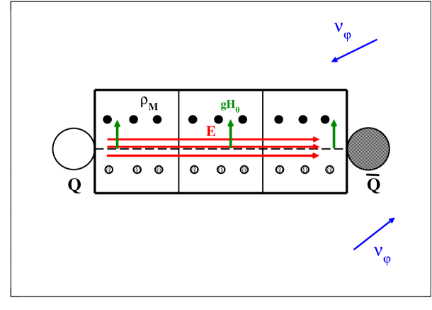
Figure 1: (Color online) Pictorial representation of the domain polarization due to a static quark-antiquark pair.

More precisely, we must admit that in a spatial region comprising the static color charges the chromomagnetic domains share the same kink plane with the domain chromomagnetic fields pointing in the same direction transverse to the kink plane. It should be clear that the polarization of the domains does not vary the energy of the wavefunctional but it increases the free energy since we lost configurational entropy. To minimize the vacuum free energy the polarization region must have the spatial volume as small as possible. Due to the symmetry of the problem, the polarization volume is a cylinder with the symmetry axis coincident with the line jointing the static color charges and with transverse sectional area of order $A_{T}\lesssim L_{D}^{2}$. The cylinder symmetry axis must lie on the common kink plane of the polarized chromomagnetic domains. This allows the polarized domains to rotate rigidly around the symmetry axis such that the increase of the vacuum free energy is reduced as much as possible. As a consequence, we are led to a modified vacuum wavefunctional as schematically illustrated in Fig. 1.
We noted in Sect. 4 that the vacuum chromomagnetic fields lead to the presence of chromomagnetic charges whose density was given by:

$$\vec{D}^{ab}(\vec{x})\,\cdot\,\vec{B}^{b}(\vec{x})\;=\;\rho^{a}_{M}(\vec{x})\;.$$ (6.15)

These chromomagnetic charges give rise to a chromomagnetic current density:

$$\vec{J}^{a}_{M}(\vec{x})\;=\;\vec{v}_{\phi}\,\rho^{a}_{M}(\vec{x})\;$$ (6.16)

where $\vec{v}_{\phi}$ is the rotational velocity of the polarized domains. Now, let us introduce cylindrical coordinate system $(x_{\ell},x_{t},\phi)$ where $x_{\ell}$ is the coordinate along the symmetry axis, $x_{t}$ the distance from the axis and $\phi$ the azimuthal angle. Evidently:

$$\vec{v}_{\phi}\;=\;v_{\phi}{\hat{\phi}}\;,$$ (6.17)

so that the azimuthal chromomagnetic current will give rise to a Lorentz force which tends to squeeze the chromoelectric fields of the static color charges into a narrow structure directed along the longitudinal direction ${\hat{x_{\ell}}}$. To do this, however, we need a chromomagnetic current density that is almost uniform along the flux tube. From the results in Sect. 4 we see that this requirement is satisfied only by the Abelian component of the chromomagnetic charge density $\rho^{3}_{M}(\vec{x})$ and $\rho^{8}_{M}(\vec{x})$. Evidently, we have:

$$\vec{J}^{\;3}_{M}(\vec{x})\;=\;\vec{v}_{\phi}\,\rho^{3}_{M}(\vec{x})\;\;,\;\;\vec{J}^{\;8}_{M}(\vec{x})\;=\;\vec{v}_{\phi}\,\rho^{8}_{M}(\vec{x})\;,$$ (6.18)

with:

$$g\rho^{3}_{M}(\vec{x})\;\simeq\;-\,\sqrt{2}\,(gH_{0})^{\frac{3}{2}}\;\,\frac{\tanh\left(\sqrt{\frac{gH_{0}}{2}}\,x_{t}\right)}{\cosh^{2}\left(\sqrt{\frac{gH_{0}}{2}}\,x_{t}\right)}\;\;,$$ (6.19)

$$g\rho^{8}_{M}(\vec{x})\;\simeq\;-\,\frac{\sqrt{3}}{2}\,(gH_{0})^{\frac{3}{2}}\;\,\frac{\tanh\left(\sqrt{\frac{gH_{0}}{4}}\,x_{t}\right)}{\cosh^{2}\left(\sqrt{\frac{gH_{0}}{4}}\,x_{t}\right)}\;\;.$$ (6.20)

Observing that the chromomagnetic current densities belong to the maximal Abelian SU(3) subgroup, the equations relating the chromomagnetic currents to the chromoelectric fields are given by the Ampere law (see, for instance, Refs. [81, 82]):

$$-\;\vec{\nabla}\;\times\vec{E}^{a}(\vec{x})\;=\;\vec{J}^{a}_{M}(\vec{x})\;\;.$$ (6.21)

From Eqs. (6.18), (6.19), (6.20) and (6.21) we get:

$$\vec{E}^{a}(\vec{x})\;\simeq\;E^{a}(x_{t})\;\hat{x}_{\ell}\;\;,$$ (6.22)

$$E^{a}(x_{t})\;\simeq\;\delta^{a3}\,E^{3}(x_{t})\;+\;\delta^{a8}\,E^{8}(x_{t})\;$$ (6.23)

with:

$$\frac{d}{dx_{t}}\,gE^{3}(x_{t})\;\simeq\;v_{\phi}\;g\rho^{3}_{M}(x_{t})\;\;,$$ (6.24)

$$\frac{d}{dx_{t}}\,gE^{8}(x_{t})\;\simeq\;v_{\phi}\;g\rho^{8}_{M}(x_{t})\;\;.$$ (6.25)

One easily obtains:

$$gE^{3}(x_{t})\;\simeq\;v_{\phi}\;gH_{0}\;\,\frac{1}{\cosh^{2}\left(\sqrt{\frac{gH_{0}}{2}}\,x_{t}\right)}\;\;,$$ (6.26)

$$gE^{8}(x_{t})\;\simeq\;\frac{\sqrt{3}}{2}\,v_{\phi}\;gH_{0}\;\,\frac{1}{\cosh^{2}\left(\sqrt{\frac{gH_{0}}{4}}\,x_{t}\right)}\;\;.$$ (6.27)

It is worth pausing to briefly recap on the origin of the chromomagnetic charge density that plays a fundamental role in the formation and structure of the chromoelectric flux tube between far apart static color charges. From the results presented in Sect. 4 it should be evident that the chromomagnetic charge densities originated from the kink structures that, in turns, come from the condensation of the tachyonic unstable modes. As discussed in details in I and in Sects. 2 and 3 of the present paper, the spin couplings of the gauge vector fields to the chromomagnetic background field generate negative mass squared terms in the lowest Landau levels. These instabilities drive the dynamical condensation of the tachyonic modes that were stabilized by the short-range repulsive interactions due to the positive quartic self-couplings of the gauge vector bosons. Albeit our calculations are based on a perturbative approach by means of a variational basis, we already remarked that the results presented in I for the SU(2) gauge theory and for SU(3) in the present paper have been corroborated by non-perturbative lattice numerical simulations of non-Abelian gauge theories in presence of external background fields [51, 52, 53, 54, 55].
The static quark-antiquark system is confined through the generation of the chromoelectric flux tube for which the quark and antiquark act as source and sink. Moreover, since the chromoelectric fields in the flux tube do not depend on the longitudinal coordinate $x_{\ell}$, we see that the quark and the antiquark at large separation distances are confined by a linearly rising potential, Eq. (6.12), with string tension given by the energy per unit length stored in the flux-tube chromoelectric fields:

$$\sigma\;\simeq\;\frac{1}{2}\;\int d\vec{x}_{t}\left\{[gE^{3}(x_{t})]^{2}\;+\;[gE^{8}(x_{t})]^{2}\right\}\;\;.$$ (6.28)

A straightforward calculation gives:

$$\sqrt{\sigma}\;\simeq\;\sqrt{5\pi J_{1}}\;v_{\phi}\;\sqrt{gH_{0}}\;,$$ (6.29)

where:

$$J_{1}\;=\;\int_{0}^{\infty}dz\;\frac{z}{\cosh^{4}z}\;\simeq\;0.295431\;\;.$$ (6.30)

We may also introduce the radius $R_{T}$ of the transverse section of the flux tube as:

$$R_{T}\;\simeq\;\;\frac{\int d\vec{x}_{t}\;|\vec{x}_{t}|\;\left\{[gE^{3}(x_{t})]^{2}\;+\;[gE^{8}(x_{t})]^{2}\right\}}{\int d\vec{x}_{t}\;\left\{[gE^{3}(x_{t})]^{2}\;+\;[gE^{8}(x_{t})]^{2}\right\}}\;\;.$$ (6.31)

We easily obtain:

$$R_{T}\;\simeq\;\;\frac{2\,\sqrt{2}\,+\,6}{5}\;\frac{J_{2}}{J_{1}}\;\frac{1}{\sqrt{gH_{0}}}\;\;,$$ (6.32)

where:

$$J_{2}\;=\;\int_{0}^{\infty}dz\;\frac{z^{2}}{\cosh^{4}z}\;\simeq\;0.214978\;\;.$$ (6.33)

An alternative definition of the transverse radius is given by $w$ where:

$$w^{2}\;\simeq\;\;\frac{\int d\vec{x}_{t}\;|\vec{x}_{t}|^{2}\;gE_{\ell}(x_{t})}{\int d\vec{x}_{t}\;gE_{\ell}(x_{t})}\;\;,$$ (6.34)

with

$$gE_{\ell}(x_{t})\;=\;gE^{3}(x_{t})\;+\;gE^{8}(x_{t})\;\;.$$ (6.35)

Performing the integrals one gets:

$$w^{2}\;\simeq\;\frac{9}{4}\;\frac{1\,+\,2\sqrt{3}}{1\,+\,\sqrt{3}}\;\frac{\zeta(3)}{\ln 2}\;\frac{1}{gH_{0}}\;\;.$$ (6.36)

It turns out that:

$$w\;\simeq\;2.0\;R_{T}\;\;.$$ (6.37)

According to Eqs. (6.26) and (6.27) the transverse profile of the flux-tube chromoelectric fields depends only on the strength of the chromomagnetic condensate $\sqrt{gH_{0}}$, while the azimuthal velocity fixes the chromoelectric field normalization. In principle, we can determine these two parameters by looking at observations. However, due to quark confinement we can only compare with theoretical experiments such as the non-perturbative numerical simulations of QCD on the lattice. In a series of paper [83, 84, 85, 86, 87, 88, 89, 90] it was investigated by lattice Monte Carlo simulations of both SU(3) pure gauge theory and (2+1)-flavor QCD at almost the physical point some properties of the chromoelectric flux tube at zero temperature generated by a static quark-antiquark pair. More precisely, these distributions were obtained from lattice measurements of the connected correlators between a plaquette and a Wilson loop. Indeed, the connected correlator provides a lattice definition of a gauge-invariant field strength tensor $gF_{\mu\nu}$ generated by the static color sources. The Wilson loop connected to the plaquette generates the static-quark color fields which point in an unknown direction $n^{a}$ in color space. The Schwinger lines connecting the Wilson loop to the plaquette perform the parallel transport of the color direction $n^{a}$ from the Wilson loop to the plaquette, so that:

$$gF_{\mu\nu}(x)\;=\;gF^{a}_{\mu\nu}(x)\,\cdot\,n^{a}\;\;.$$ (6.38)

Equation (6.38) is an inevitable consequence of the gauge invariance of the lattice operator and its linear dependence on the color fields in the continuum limit has been explicitly tested in Ref. [86] (see Fig. 3 there). Remarkably, extensive lattice simulations showed that, far from the sources, the flux tube is almost completely formed by the longitudinal chromoelectric field $gE_{\ell}$ which is constant along the flux tube and decreases rapidly in the transverse direction $x_{t}$. Introducing (here $\beta$ is the lattice gauge coupling):

$$E_{\ell}(x)\;=\;\sqrt{\frac{\beta}{6}}\;\,gE_{\ell}(x)\;\;,$$ (6.39)

the formation of the longitudinal chromoelectric field $E_{\ell}(x)$ was interpreted as the dual Meissner effect within the dual superconductor mechanism of quark confinement. Accordingly, the lattice data for the longitudinal chromoelectric field were analyzed by exploiting a variational model for the magnitude of the normalized order parameter of an isolated vortex in type II superconductors advanced in Ref. [91]. As a consequence, the transverse distribution of the chromoelectric flux tube were described according to:

$$E_{\ell}(x_{t})\;=\;\frac{\varphi}{2\pi}\;\frac{1}{\lambda\,\xi_{v}}\;\frac{K_{0}(\sqrt{x_{t}^{2}\,+\,\xi_{v}^{2})}}{K_{1}(\frac{\xi_{v}}{\lambda})}\;\;,$$ (6.40)

where $\xi_{v}$ is a variational core-radius parameter, $\lambda$ is the penetration length and $K_{n}(x)$ is the modified Bessel function of order $n$. Moreover, the so-called Ginzburg-Landau parameter $\kappa_{GL}$ can be obtained by:

$$\kappa_{GL}\;=\;\frac{\lambda}{\xi}\;=\;\sqrt{2}\;\,\frac{\lambda}{\xi_{v}}\;\left[1\;-\;\frac{K_{0}^{2}(\frac{\xi_{v}}{\lambda})}{K_{1}^{2}(\frac{\xi_{v}}{\lambda})}\right]^{\frac{1}{2}}\;\;,$$ (6.41)

$\xi$ being the coherence length.
It resulted that the phenomenological law Eq.(6.40) allowed to track very well the transverse profile of the longitudinal chromoelectric field giving support to the dual superconductor mechanism of quark confinement. On the other hand, our attempt to unveil from first principles the structure of the large-scale QCD vacuum led us to a completely different picture for the formation of the color flux tube generated by static sources. According to our previous discussion, the chromoelectric flux tube is mainly composed by the Abelian component $gE^{3}$ and $gE^{8}$. Therefore, we can safely assume that:

$$gE^{a}(x)\,\cdot\,n^{a}\;\simeq\;gE^{3}(x)\;+\;gE^{8}(x)$$ (6.42)

where $gE^{3}(x)$ and $gE^{8}(x)$ are explicitly given by Eqs. (6.26) and (6.27). So that we have for the measured chromoelectric longitudinal field:

$$E_{\ell}(x_{t})\;\simeq\;v_{\phi}\;gH_{0}\;\left\{\,\frac{1}{\cosh^{2}\left(\sqrt{\frac{gH_{0}}{2}}\,x_{t}\right)}\;+\;\frac{\sqrt{3}}{2}\;\frac{1}{\cosh^{2}\left(\sqrt{\frac{gH_{0}}{4}}\,x_{t}\right)}\right\}\;\;.$$ (6.43)

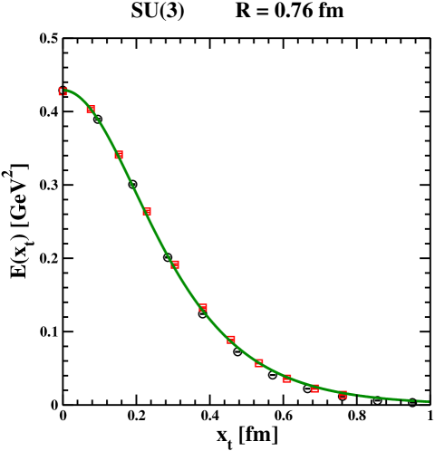
Figure 2: (Color online) The longitudinal chromoelectric field versus the transverse distance for SU(3) at $\beta=6.050$ (circles) and $\beta=6.195$ (squares). The data have been taken from Fig. 3, left panel, of Ref. [87]. The continuous line is Eq. (6.43) with parameters given by Eq. (6.44).

In Eq. (6.43) we considered that $\sqrt{\frac{\beta}{6}}\approx 1$ and that the smearing procedure needed to extract the physical informations from the measured lattice connected correlator leads to an effective non-perturbative finite renormalization of the field strength tensor. As a consequence, in Eq. (6.43) it is intended the presence of an unknown renormalization constant that, however, affects only the value of the longitudinal chromoelectric field at $x_{t}=0$. A remarkable consequence of Eq. (6.43) is that the transverse profile of the longitudinal chromoelectric field depends only on the vacuum chromomagnetic condensate strength $\sqrt{gH_{0}}$. For comparison, the Clem’s ansatz Eq. (6.40) needs two parameters $\lambda$ and $\xi_{v}$ to track the transverse profile.
We have contrasted Eq. (6.43) to several lattice measurements of the longitudinal chromoelectric field and, surprisingly, we found that Eq. (6.43) is able to reproduce the transverse profiles of $E_{\ell}(x_{t})$ quite well. To better appreciate this last point, in Fig. 2 we display the behaviour of the longitudinal chromoelectric field as a function of the transverse distance for two different values of the gauge coupling for the SU(3) pure gauge theory as reported in Fig. 3, left panel, of Ref. [87]. In Ref. [87] the lattice data for $E_{\ell}(x_{t})$ were nicely fitted by the Clem’s ansatz Eq. (6.40). Likewise, we find that the transverse profile of the longitudinal chromoelectric field can be accounted for by using Eq. (6.43) with (see Fig. 2):

$$v_{\phi}\;\simeq\;0.21\;\;,\;\;\sqrt{gH_{0}}\;\simeq\;1.05\;\text{GeV}\;\;.$$ (6.44)

However, in Refs. [88, 89] it was enlighten the presence of an effective Coulomb-like chromoelectric field $\vec{E}^{C}$ associated with the static quark sources. Indeed, we have said that it is conceivable by quantum tunnelling the formation of bubbles of perturbative vacuum around the static color sources with a linear size of order the chromomagnetic length. So that near the static charges there is a perturbative Coulomb chromoelectric field that, however, may penetrate at larger distances due to the restoration of color coherence along the flux tube. Therefore, the measured chromoelectric field $\vec{E}$ can be written as [88, 89]:

$$\vec{E}\;=\;\vec{E}^{NP}\;+\;\vec{E}^{C}\;\;$$ (6.45)

with the non-perturbative chromoelectric field $\vec{E}^{NP}$ being purely longitudinal. In other words, $\vec{E}^{NP}$ must be identified with the confining field of the QCD flux tube. Following Ref. [89], in Fig. 3, left panel we display the transverse profile of the non-perturbative chromoelectric field for the SU(3) pure gauge theory corresponding to a source distance of $R\simeq 0.85$ fm. The transverse profile is consistent with Eq. (6.43) with (solid line in Fig. 3):

$$v_{\phi}\;\simeq\;0.185\;\;,\;\;\sqrt{gH_{0}}\;\simeq\;1.0\;\text{GeV}\;\;,\;\;\sqrt{\sigma}\;\simeq\;398.5\;\text{MeV}\;\;.$$ (6.46)

In Eq. (6.46) the string tension has been evaluated by means of Eq. (6.29). Note that the value of the string tension in Eq. (6.46) is smaller with respect to the accepted value Eq. (6.13). This is to be expected for we have already noticed that there is a non-perturbative renormalization constant due to the smearing procedure that affects the measured chromoelectric field. Such a renormalization constant can be easily evaluated from the ratio of the estimate of the string tension in Eq. (6.46) to the reference value given by Eq. (6.13).
We saw that the connected correlators allow to extract the gauge-invariant flux-tube field strength tensor $F_{\mu\nu}$. In Ref. [89] from the field strength tensor it was constructed a stress energy-momentum tensor $T_{\mu\nu}(x)$ having the Maxwell form. In fact, in the Appendix A of Ref. [89] the energy-momentum tensor $T_{\mu\nu}$ was considered as a function of the field strength tensor $F_{\mu\nu}$ characterizing the color flux tube. Assuming that the field strength tensor points in a single color direction parallel to the color direction of the static sources, it follows that the energy-momentum tensor lies in the same single color direction and, therefore, it has the Maxwell form [89]:

$$T_{\mu\nu}(x)\;=\;F_{\mu\alpha}(x)F_{\alpha\nu}(x)\;-\;\frac{1}{4}\,g_{\mu\nu}\,F_{\alpha\beta}(x)F_{\alpha\beta}(x)\;\;.$$ (6.47)

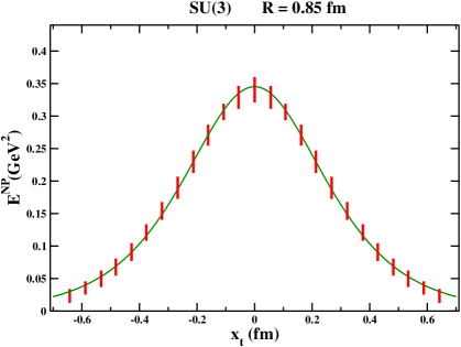
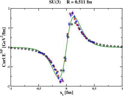
Figure 3: (Color online) Left panel. Transverse distribution of the non-perturbative flux-tube chromoelectric field. The vertical bars mark the values of the chromoelectric field as the longitudinal coordinate varies along the flux tube. The data have been taken from Fig. 5 in Ref. [89]. The solid line is the fit to the data using Eq. (6.46). Right panel. The transverse distribution of the rotational of the non-perturbative chromoelectric field for three different valuues of the gauge coupling, $\beta=6.240$ (circles), $\beta=6.544$ (squares) and $\beta=6.769$ (diamonds). The data have been taken from Fig. 5 in Ref. [90]. The solid line is the chromomagnetic current given by Eq, (6.49) by assuming $\sqrt{gH_{0}}\simeq 1.5$ GeV.

However, we have shown that the field strength tensor is mainly composed by the Abelian color directions $a=3,8$. Nevertheless, the Abelian nature of the flux-tube field strength tensor fully justify the Maxwell construction proposed in Ref. [89]. More recently, in Ref. [90] it was presented for the first time the evidence of a solenoidal chromomagnetic current responsible for the formation of the longitudinal chromoelectric field. The chromomagnetic current density was defined by the Ampere law:

$$\vec{J}_{mag}(\vec{x})\;=\;\vec{\nabla}\;\times\;\vec{E}(\vec{x})\;=\;\vec{\nabla}\;\times\vec{E}^{NP}(\vec{x})\;,$$ (6.48)

where we used $\vec{\nabla}\,\times\,\vec{E}^{C}(\vec{x})=0$. Comparing Eq. (6.48) with our Eq. (6.21) we infer that:

$$\vec{J}_{mag}(\vec{x})\;=\;-\left[\vec{J}^{3}_{M}(\vec{x})+\vec{J}^{8}_{M}(\vec{x})\right]$$ (6.49)

with $\vec{J}^{3,8}_{M}(\vec{x})$ given by Eqs. (6.18), (6.19) and (6.20). In Fig. 3, right panel, we report the chromomagnetic current, Eq. (6.48), for three different values of the gauge coupling evaluated at the transverse plane at a distance $\frac{R}{4}$ from the source. The data have been reproduced from Fig. 5 in Ref. [90]. Since the distance between the static sources is rather small ($R\simeq 0.511$ fm) the data seem to display some noticeable scattering probably due to systematic effects arising from the subtraction of the Coulomb field from the measured flux-tube chromoelectric field. Nevertheless, our theoretical chromomagnetic current seem to track reasonably well the lattice data.
In our opinion, the essential Abelian nature of the chromomagnetic currents and the ensuing flux-tube chromoelectric fields are at the heart of the so-called Abelian dominance observed in several lattice simulations [8, 10, 16]. Indeed, the dual superconductivity scenario is realized by adopting a gauge-fixing procedure analogous to the unitary gauge where a suitable matrix-valued operator is diagonalized leaving unfixed the maximal Abelian subgroup U(1)$\times$U(1) whose generators belong to the Cartan subalgebra of the SU(3) gauge group. In these gauges the given gauge theory can be thought of as an essentially Abelian gauge theory. Our previous results should make evident that the observed Abelian dominance is not the cause but it is a consequence of the structure of the confining quantum vacuum.
It is interesting to also check if our theoretical transverse shape of the flux-tube chromoelectric field is consistent with numerical studies in QCD with maximal Abelian gauge fixing.

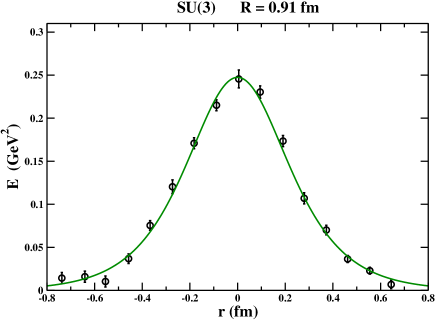
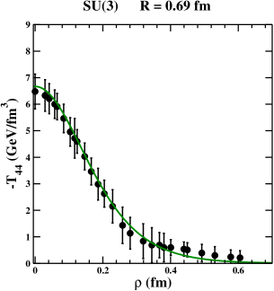
Figure 4: (Color online) Left panel. Transverse distribution of the Abelian chromoelectric field generated by a static quark-antiquark pair at distance $R\simeq 0.91$ fm in quenched QCD in the maximal Abelian gauge. The data have been taken form Fig. 15 in Ref. [92]. The continuous line is Eq. (6.43) with parameters given by Eq. (6.50). Right panel. The transverse distribution at the mid transverse plane of the energy density around a static quark-antiquark pair. The data have been extracted from Fig. 3, panel (b), in Ref. [93]. The continuous line corresponds to Eq. (6.51) with parameters given by Eq. (6.52).

As a matter of fact, in Fig. 4, left panel, we report the profile of the Abelian flux tube chromoelectric field (in physical units) in quenched QCD in the maximal Abelian gauge as displayed in Fig. 15 of Ref. [92] together with our theoretical transverse profile, Eq. (6.43) with:

$$v_{\phi}\;\simeq\;0.102\;\;,\;\;\sqrt{gH_{0}}\;\simeq\;1.14\;\text{GeV}\;\;.$$ (6.50)

We can see that, also in this case, our theoretical expectations are able to track quite well the lattice data.
As the last check, we focus, now, on several numerical studies of the pure gauge SU(3) theory on the the structure of the static quark flux tube implemented with correlators between Wilson loops and plaquettes. In this case, in general, the lattice observables give informations on the square of the flux-tube field strength tensor. For definitiveness, we have considered the quite recent studies on the spatial distribution of the stress energy-momentum tensor around a static quark-antiquark color sources reported in Ref. [93]. The authors of Ref. [93] investigated the spatial distribution of the stress energy-momentum tensor $T_{\mu\nu}$ around a static quark-antiquark pair in the SU(3) pure gauge theory. To smooth the gauge field configurations it was employed the Yang-Mills gradient flow (for a recent review see, eg, Ref. [94] and references therein). The spatial distribution of the static color source energy-momentum tensor was obtained by measuring the correlators of the conserved renormalized stress tensor [95] and a Wilson loop. It is worth mentioning that in Appendix A of Ref. [89] it was showed that the Maxwell energy-momentum tensor built from the field strength tensor characterizing the SU(3) flux tube resulted to be in satisfying agreements with the results presented in Ref. [93]. For a more quantitative comparison we looked at the transverse distribution of the flux-tube energy density ${\cal{E}}(x)=-\,T_{44}(x)$ measured at the mid transverse plane and displayed in Fig. 3 of Ref. [93]. According to our results we should have:

$$-\,T_{44}\;\simeq\;\frac{1}{2}\;\left\{[gE^{3}(r)]^{2}\;+\;[gE^{8}(r)]^{2}\right\}\;$$ (6.51)

where $r$ is the transverse distance in the cylindrical coordinate system. The fit of Eq. (6.51) to the lattice data returned (see Fig. 4, right panel):

$$v_{\phi}\;\simeq\;0.20\;\;,\;\;\sqrt{gH_{0}}\;\simeq\;1.10\;\text{GeV}\;\;,\;\;\sqrt{\sigma}\;\simeq\;474\;\text{MeV}\;.$$ (6.52)

Again, we see that the lattice data are in quite good agreement with theoretical expectations. Furthermore, we note that the estimate of the string tension in Eq. (6.52) is in accordance with the large $R$ behaviour of the quark-antiquark force, displayed in Fig. 4 of Ref. [93], as directly determined from the Wilson loops and the renormalized energy-momentum tensor as well as with the string tension reference value Eq. (6.13), signalling that the renormalized lattice energy-momentum tensor does not need further non-perturbative renormalization since it is expected to have a smooth continuum limit [95].
To summarize, we have shown that our picture for the formation of a chromoelectric squeezed flux tube generated by a static quark-antiquark pair in the SU(3) pure gauge theory turned out to be in reasonable agreement with lattice outcomes from different collaborations. Our previous discussion leads to the following estimate for the strength of the vacuum chromomagnetic condensate in the pure gauge SU(3) theory:

$$\sqrt{gH_{0}}\;\simeq\;1.0\;-\;1.1\;\text{GeV}\;\;\;\;\;\;\text{SU(3)}\;.$$ (6.53)

From this last equation we may estimate the flux-tube transverse radius, Eq. (6.32), $R_{T}\,\simeq\,0.2$ fm, or the width, Eq. (6.37), $w\,\simeq\,0.4$ fm in agreement with several lattice determinations.
Up to now we have dealt with only the SU(3) gluon fields and completely neglected the dynamical role of the fermion fields. Although this point will be addressed in more details in the following Section, it is, nevertheless, worthwhile to ascertain how dynamical quarks affect the structure of the chromoelectric fields generated by a static quark-antiquark pair. Indeed, we looked at lattice studies in full QCD on the flux-tube color fields and in Fig. 5 we present the transverse distribution of the longitudinal flux-tube chromoelectric field as obtained by three different lattice group.

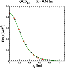
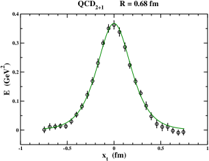
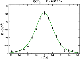
Figure 5: (Color online) The transverse shape of the flux-tube longitudinal chromoelectric field in full QCD. The continuous lines are qualitative fits of the lattice data to our Eq. (6.43).

Firstly, in Fig. 5, left panel, it is displayed the behaviour of the longitudinal chromoelectric field versus the transverse distance as obtained from two different values of the gauge coupling, $\beta=6.743$ (circles) and $\beta=6.885$ (squares), for (2+1)-flavours QCD with HISQ/Tree action [87]. The data was obtained on the line of constant physics by adjusting the gauge coupling and the bare quark masses so as to keep the strange quark mass fixed at the physical point and the light quark masses corresponding to a pion mass $m_{\pi}\simeq 160$ MeV. The data have been extracted from Fig. 3, right panel, in Ref. [87]. The continuous line corresponds to Eq. (6.43) with:

$$v_{\phi}\;\simeq\;0.17\;\;,\;\;\sqrt{gH_{0}}\;\simeq\;1.17\;\text{GeV}\;\;.$$ (6.54)

In Fig. 5, middle panel, we report the transverse profile of the flux-tube chromoelectric field reported in Fig. 14 of Ref. [96], where the flux tube properties were investigated by numerical lattice simulations for full QCD with (2+1)-flavours of stoud-improved staggered fermions with physical quark masses (pion mass $m_{\pi}\simeq 135$ MeV). In this case we found (continuous line in Fig. 5):

$$v_{\phi}\;\simeq\;0.108\;\;,\;\;\sqrt{gH_{0}}\;\simeq\;1.35\;\text{GeV}\;\;.$$ (6.55)

Finally, in Fig. 5, right panel, we consider the transverse distribution of the flux-tube chromoelectric field for QCD in the maximal Abelian gauge with two degenerate non-perturbatively improved Wilson fermions with a rather heavy mass $m_{q}\simeq 100$ MeV [92]. Fitting the lattice data to our Eq. (6.43) we get:

$$v_{\phi}\;\simeq\;0.104\;\;,\;\;\sqrt{gH_{0}}\;\simeq\;1.15\;\text{GeV}\;\;.$$ (6.56)

It is remarkable that, in accordance with common expectations, the inclusion of dynamical quarks does not substantially modify the color structure of the flux tube. The only effect seems to be a small increase of the chromomagnetic condensate strength:

$$\sqrt{gH_{0}}\;\simeq\;1.2\;-\;1.3\;\text{GeV}\;\;\;\;\;\;\text{QCD}\;.$$ (6.57)

Our quantum vacuum functional leads us to reach a clear picture on the flux-tube physics. Indeed, the squeezing of the chromoelectric fields generated by a static quark-antiquark pair is due to chromomagnetic currents belonging to the maximal Abelian subgroup of SU(3) whose transverse distribution only depends on the strength of the vacuum chromomagnetic condensate. It is remarkable that the resulting flux-tube chromoelectric fields are obtained by solving the quite simple Ampere law, Eq. (6.21). Evidently, the qualitative agreement of our theoretical expectations to several lattice measurements leads us to believe that we are on the right path. Undoubtedly, the knowledge of the color structure and distribution of the flux-tube has several interesting phenomenological consequences. Here we restrict ourself to the comparison with the seminal paper by Casher, Neuberger and Nussinov [97] that lies at the basis of several high-energy physics Monte Carlo codes. In Ref. [97] quark confinement is assumed to be generated by the formation of chromoelectric flux tubes with almost uniform energy density. By employing the approximations where the chromoelectric field which develops between the quarks is assumed to be an almost classical field, the authors of Ref. [97] found that the flux-tube chromoelectric field is pratically longitudinal. Moreover, to estimate the production of quark pairs in the flux tubes it is assumed that the longitudinal chromoelectric field is Abelian:

$$gE^{a}\;\simeq\;\delta^{a3}\,gE^{3}\;+\;\delta^{a8}\,gE^{8}\;.$$ (6.58)

Using the Gauss law and:

$$\frac{1}{2}\;A_{T}\;\sum_{a=1}^{8}\left(E^{a}\right)^{2}\;\simeq\sigma\;$$ (6.59)

where $A_{T}\simeq\pi R_{T}^{2}$ is the cross sectional area, one gets:

$$\frac{1}{2}\;gE^{3}\;\simeq\;\frac{3}{2}\;\sigma\;\;,\;\;gE^{8}\;\simeq\;\frac{1}{\sqrt{3}}\;gE^{3}\;.$$ (6.60)

Within the above framework, the quark dynamics into the flux tube may be approximately described by the Dirac equation in presence of a classical almost uniform longitudinal chromoelectric field given by a diagonal matrix in color space [97]:

$$\left[-\;i\,\not{\partial}\;-\;m_{eff}\;-\;2\;i\;\sigma\,z\;\begin{pmatrix}1&&\\ &-\frac{1}{2}&\\ &&-\frac{1}{2}\end{pmatrix}\right]\;\psi\;=0\;\;,$$ (6.61)

where $m_{eff}$ is the effective quark mass and $z$ is our longitudinal coordinate $x_{\ell}$. After that, the dynamical process of quark pair creation may be described rather well by the well-known Schwinger mechanism [98, 99].
It is remarkable that within our approach we have confirmed the Abelian structure of the flux-tube chromoelectric fields. More precisely, the chromoelectric fields that confine the static quark-antiquark pair is longitudinal and it is almost completely formed by the $a=3,8$ color directions. However, if we assume an uniform flux-tube, instead of Eq. (6.60) we obtain:

$$gE^{8}(x_{t}=0)\;\simeq\;\frac{2}{\sqrt{3}}\;gE^{3}(x_{t}=0)\;,$$ (6.62)

and

$$gE^{3}(x_{t}=0)\;\simeq\;v_{\phi}\,gH_{0}\;\simeq\;\frac{\sigma}{5\pi J_{1}v_{\phi}}\;\simeq\;1.08\,\sigma\;,$$ (6.63)

where we used Eq. (6.29) and assumed $v_{\phi}\simeq 0.2$. As a consequence we are led to the following Dirac equation:

$$\left[-\;i\,\not{\partial}\;-\;m_{eff}\;-\;1.08\;i\;\sigma\,z\;\begin{pmatrix}1&&\\ &-\frac{1}{3}&\\ &&-\frac{2}{3}\end{pmatrix}\right]\;\psi\;=0\;\;.$$ (6.64)

In addition, it is interesting to note that we may go beyond the approximations adopted in Ref. [97] for we have an explicit expression for the transverse distribution of the flux-tube chromoelectric fields. In fact, the transverse profile of the chromoelectric fields allows, in principle, to determine the transverse distribution of the quark-antiquark pairs produced by the Schwinger mechanism ( for a good account see, eg, Ref. [100] and references therein), however such matter goes beyond the aim of the present paper.
Let us conclude this rather lengthy Section by discussing the remarkable color Meissner effect [31, 32, 33, 34] that led us to picture the QCD vacuum like a chromomagnetic condensate. In order to investigate non-perturbatively the quantum vacuum structure in Refs. [28, 29, 30], by means of the so-called Schrödinger functional, it was introduced a gauge-invariant effective action for gauge systems in external static background fields. In particular, it was enlightened that the deconfinement temperature depends on the strength of an external Abelian chromomagnetic field in both the pure SU(3) gauge theory [31, 32, 33] and QCD with two degenerate staggered dynamical quarks [34]. Actually, it was ascertained that the deconfinement temperature decreases when the strength of the applied field is increased and eventually goes to zero. Indeed, in Fig. 6 we display the critical temperature of deconfinement versus the strength of the applied chromomagnetic field for SU(3) (left panel) and QCD (right panel). For the pure gauge theory the data have been taken from Fig. 4 in Ref. [32] taking into account that $T_{c}\,=\,300(7)$ MeV [101], while for QCD with two dynamical staggered quarks with a rather large mass (pion mass $m_{\pi}$ around 500 MeV) the data have been extracted from Fig. 7 of Ref. [34] assuming $T_{c}~{}\simeq~{}170$ MeV. From Fig. 6 we infer that in both cases the deconfinement critical temperature decreases linearly with $\sqrt{gH}$. In fact, the lattice data can be fitted to Eq. (1.1) giving (see the continuous lines in Fig. 6):

Figure 6: (Color online) Behaviour of the deconfinement critical temperature versus the strength of the external chromomagnetic firld for SU(3) pure gauge theory (left panel) and QCD with two degenerate staggered quarks (right panel). The continuous lines are the best fits of the lattice data to Eq. (1.1).

$$T_{c}(0)\;=\;298(10)\;\text{MeV}\;\;,\;\;\sqrt{gH_{c}}\;=\;1.22(4)\;\text{GeV}\;\;\;\;\;\;\text{SU(3)}\;,$$ (6.65)

$$T_{c}(0)\;=\;170(12)\;\text{MeV}\;\;,\;\;\sqrt{gH_{c}}\;=\;1.61(14)\;\text{GeV}\;\;\;\;\;\;\text{QCD}\;.$$ (6.66)

From a dynamical point of view these peculiar behaviours of the critical temperatures point to the prevalent role of the chromomagnetic length. Actually, we may now try to interpret the color Meissner effect within our picture of the confining vacuum wavefunctional. Firstly, we note that the gauge systems was probed with external fields whose strengths $\sqrt{gH}$ was smaller than $\sqrt{gH_{0}}$, Eqs. (6.53) and (6.57). So that it is conceivable that the main effects of the applied chromomagnetic fields are to polarize the chromomagnetic domains such that the vacuum chromomagnetic condensate tends to lie in the same direction as the external field. As a consequence, we see that the polarization effects cause an increase of the effective domain size leading to a decrease of the mass gap $\Delta\sim\frac{1}{L_{D}}$. Since on dimensional ground the deconfinement temperature $T_{c}$ is of order of the mass gap, we may explain the observed decreases of the critical temperature $T_{c}(gH)$. If this interpretation is correct, then at the critical strength $\sqrt{gH_{c}}\sim\sqrt{gH_{0}}$ the gauge system undergoes a quantum deconfinement phase transition. However, the deconfined phase is far from being similar to a weakly interacting gas of quarks and gluons, but it should resemble the quantum Hall liquid of the condensed matter physics. A clear signature of this would come from the measurements of the chromoelectric fields generated by a static quark-antiquark pair immersed in an uniform chromomagnetic field. Indeed, at $T=0$ and $\sqrt{gH}>\sqrt{gH_{c}}$ we lost confinement due to the absence of a mass gap and the instauration of long-range color correlations. However, since the quantum vacuum is characterized by polarized chromomagnetic domains we expect that the formation of a squeezed flux tube with a non-zero string tension when the static-source joining line is perpendicular to the external field, $\sqrt{\sigma_{T}}\simeq\sqrt{\sigma}$. On the other hand, for a static quark-antiquark pair in the direction parallel to the external field the formation of the flux tube should be strongly suppressed leading to $\sqrt{\sigma_{L}}\simeq 0$. Unfortunately, in the literature there are no lattice data that could support the above scenario. However, quite recently such an investigation has been presented in Ref. [96] for full QCD with (2+1)-flavour at the physical point immersed in extremely strong magnetic fields. Actually, the influence of external magnetic background fields on QCD has attracted growing interest in recent years (see, for instance, Refs. [102, 103, 104, 105] and references therein).
Quantum chromodynamics with background magnetic fields can be studied directly by means of non-perturbative lattice simulations. Continuum extrapolated results employing improved staggered quarks with physical masses have been used to map out the QCD phase diagram up to field strength $eB=9\,\text{GeV}^{2}$. It turned out that the applied magnetic field increases the light quark condensate in the confined phase. This enhancement has been called magnetic catalysis. On the contrary, in the transition region from the confined phase to the deconfined one the light quark condensate seems to decrease leading to the so-called inverse magnetic catalysis. It is important to stress that the chiral and deconfinement critical temperatures alway coincide as happened in absence of the external magnetic fields. Moreover, as a result of the non-monotonous dependence of the light quark condensate on the magnetic field strength and temperature, $T_{c}(eB)$ is reduced by the magnetic field.
It is widely believed that the mechanisms behind the magnetic catalysis are quite transparent and these can be understood in terms of the dimensional reduction of the gauge system and the high degeneracy of the lowest Landau levels. Unfortunately, theoretical predictions are in reasonable agreement with the lattice data only for not too strong magnetic fields, $eB\lesssim 0.3\;\text{GeV}^{2}$. On the contrary, we feel that there is a more mundane explanation of the magnetic catalysis at least in the confined phase. Indeed, one must bring in mind that in the QCD confined phase the physical states are colorless hadrons. Considering that an external magnetic field is coupled to the gauge system through the electromagnetic vector current, we may employ the old vector meson dominance idea to argue that the electromagnetic current is mainly coupled to vector mesons. Moreover, long time ago in Ref. [106] it was proved the duality relation between quark-antiquark bound states and asymptotically free quarks by using relativistic wave functions and couplings to both vector and axial current. Within these approximations we were able to evaluate as an external constant magnetic field contributes to the vacuum energy density and, thereby, the zero-temperature renormalized chiral condensate as usually measured in numerical lattice simulations:

$$\Sigma_{ud}(eB,T)\;=\;\frac{m_{ud}}{m_{\pi}^{4}}\;\left\{<\psi\bar{\psi}>(eB,T)\;-\;<\psi\bar{\psi}>(0,0)\right\}\;.$$ (6.67)

Interestingly enough, we found that our theoretical estimate was in rather good agreement with the lattice data [107, 109, 96] for the average chiral condensate $\frac{1}{2}~{}[\Sigma_{u}(eB,0)~{}+~{}\Sigma_{d}(eB,0)]$ in the whole range of applied magnetic fields $eB\,\leq\,9\,\text{GeV}^{2}$. Moreover, we also checked that our theoretical results were able to track quite well the behaviour of $\frac{1}{2}~{}[\Sigma_{u}(eB,0)~{}-~{}\Sigma_{d}(eB,0)]$ versus $eB$ as reported in Ref. [107]. We have, also, evaluated the thermal corrections and found satisfying agreement with the continuum extrapolated lattice results  [107] in the confined phase. On the other hand, it should be evident that to understand the inverse magnetic catalysis it is necessary to unravel the nature of the deconfined QCD vacuum in presence of external magnetic fields. To do this, it is mandatory to try to explain the behaviour of the critical deconfinement temperature as a function of the strength of the external magnetic field.

Figure 7: The lattice data for the deconfinement temperature versus the strength of the external magnetic field $\sqrt{eB}$. The continuous line is our fit of the data to Eq. (6.68) for $eB\,\leq\,3.25\,\text{GeV}^{2}$, the dashed line is the fit to Eq. (6.71) for $eB\,\geq\,3.25\,\text{GeV}^{2}$.

To this end, in Fig. 7 we display the deconfinement temperature versus $\sqrt{eB}$. The lattice data have been taken from Fig. 9, left upper panel, in Ref. [108] for $eB\,\lesssim 1\;\text{GeV}^{2}$, from Ref. [109] at $eB\,=\,3.25\;\text{GeV}^{2}$ and from Ref. [110] at $eB\,=\,4,9\;\text{GeV}^{2}$. Looking at Fig. 7 we see that the behaviour of the deconfinement temperature clearly indicates the presence of two different regimes. For not to strong magnetic fields $T_{c}(eB)$ smoothly decreases by increasing the strength of the applied magnetic field and it seems to saturate in the limit $eB\,\rightarrow\infty$. We agree with the discussion presented in Ref. [109] where this effect is ascribed to the explicit breaking of the rotational symmetry by the external magnetic field and the expected dimensional reduction in the quark sector. Indeed, from the structure of the gluon propagator in very strong magnetic fields (see Ref. [103] and references therein) one argues that the limiting effective gauge theory corresponds to an anisotropic pure gauge theory due to the enhancement of the chromo-dielectric constant. This qualitatively explains the small reduction of the deconfinement temperature and the saturation to an asymptotic value since for very strong magnetic fields the fermions are expected to be frozen into the lowest Landau levels. Accordingly, in Ref. [109] the lattice data were fitted to the phenomenological law:

$$T_{c}(eB)\;=\;T_{c}(0)\,\frac{1\;+\;a_{1}\,(eB)^{2}}{1\;+\;a_{2}\,(eB)^{2}}\;\;.$$ (6.68)

In fact, for $eB\,\leq\,3.25\;\text{GeV}^{2}$ the data are very well described by Eq. (6.68) with [109]:

$$T_{c}(0)\;=\;160(2)\;\text{MeV}\;\;,\;\;a_{1}\;=\;0.54(2)\;\;,\;\;a_{2}\;=\;0.82(2)\;\;.$$ (6.69)

As a consistency check, we have fitted the data displayed in Fig. 7 to Eq. (6.68) and found:

$$T_{c}(0)\;=\;159.9(1.5)\;\text{MeV}\;\;,\;\;a_{1}\;=\;0.55(15)\;\;,\;\;a_{2}\;=\;0.83(19)\;\;.$$ (6.70)

It is reassuring to see that our fit is perfectly consistent with Eq. (6.69) albeit with larger errors.
However, more recent studies presented in Ref. [110] found that the critical deconfinement temperatures suffer a further decrease in extremely strong magnetic fields $eB\,=\,4,\,9\;\text{GeV}^{2}$ (see Fig. 7). This kind of behaviour cannot be explained by the screening effects for we already argued that the quarks are frozen into the lowest Landau levels. However, we may offer a plausible explanation within our picture of the QCD vacuum as a disordered chromomagnetic condensate. We rely on the one-loop calculations of the effective potential in QCD in external Abelian chromomagnetic and magnetic fields [111]. In fact, the chromomagnetic and magnetic fields are coupled to each other through the quark loops such that the vacuum energy is minimized if the external fields lie in the same direction. This means that external magnetic fields tend to polarize the chromomagnetic domains of our QCD vacuum. As a consequence, according to our previous discussion for the SU(3) pure gauge theory, we are led to expect the presence of the Meissner effect where the critical deconfinement temperature should decrease according to:

$$T_{c}(eB)\;=\;T_{c}(0)\,\left[1\;-\;\frac{\sqrt{eB}}{\sqrt{eB_{c}}}\right]\;\;.$$ (6.71)

Actually, we find the the lattice data are consistent with Eq. (6.71) for $eB\,\gtrsim\,3\;\text{GeV}^{2}$ (see the dashed line in Fig. 7):

$$T_{c}(0)\;=\;160.2(3.7)\;\text{MeV}\;\;,\;\;\sqrt{eB_{c}}\;=\;5.28(31)\;\text{GeV}^{2}\;\;.$$ (6.72)

A further indirect confirmation of our picture comes from the fact that at $eB\,=\,9\;\text{GeV}^{2}$ the deconfinement transition turns into a first-order transition as in the pure gauge theory [110]. We may, now, gain further insight on the nature of the quantum vacuum by looking at the structure of the flux-tube chromoelectric fields. Remarkably, the authors of Ref. [96] investigated the transverse profile of the longitudinal chromoelectric field generated by static quark-antiquark pair directed along the applied external magnetic field (longitudinal flux tube) as well as perpendicular to the magnetic field (transverse flux tube).

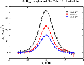
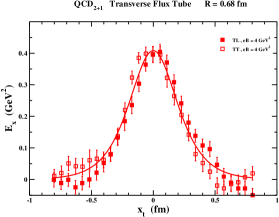
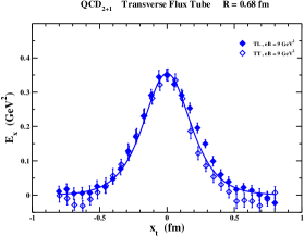
Figure 8: (Color online) Transverse profile of the flux-tube chromoelectric field for $eB\,=\,0,\;4,\,9\;\text{GeV}^{2}$; left panel, longitudinal flux tubes, middle e right panels, transverse flux tubes. The data have been taken from Figs. 10, 11 and 14 in Ref. [96] corresponding to a lattice size $a\,=\,0.0572$ fm. We use the same nomenclature as in Ref. [96].

In Fig. 8 we display the profile of the chromoelectric field for longitudinal and transverse flux tubes for three different values of the external magnetic field. Note that for $eB=0$ the lattice data have been already displayed in Fig. 5, middle panel. From the fit to our Eq. (6.43) we obtained:

$$\text{eB}\;=\;0:\;v_{\phi}\;\simeq\;0.108\;\;,\;\;\sqrt{gH_{0}}\;\simeq\;1.35\;\text{GeV}\;\;,\;\;\sqrt{\sigma}\;\simeq\;314\;\text{MeV}$$ (6.73)

where for the string tension we are using Eqs. (6.29) and (6.30). Likewise, we get for the longitudinal flux tube (L):

$$\text{eB}\;=\;4\;\text{GeV}^{2}:\;v_{\phi}\;\simeq\;0.051\;\;,\;\;\sqrt{gH_{0}}\;\simeq\;1.55\;\text{GeV}\;\;,\;\;\sqrt{\sigma}\;\simeq\;170\;\text{MeV}\;,$$ (6.74)

$$\text{eB}\;=\;9\;\text{GeV}^{2}:\;v_{\phi}\;\simeq\;0.034\;\;,\;\;\sqrt{gH_{0}}\;\simeq\;1.55\;\text{GeV}\;\;,\;\;\sqrt{\sigma}\;\simeq\;113\;\text{MeV}\;,$$ (6.75)

while for the transverse flux tubes (TT, TL):

$$\text{eB}\;=\;4\;\text{GeV}^{2}:\;v_{\phi}\;\simeq\;0.14\;\;,\;\;\sqrt{gH_{0}}\;\simeq\;1.25\;\text{GeV}\;\;,\;\;\sqrt{\sigma}\;\simeq\;370\;\text{MeV}\;,$$ (6.76)

$$\text{eB}\;=\;9\;\text{GeV}^{2}:\;v_{\phi}\;\simeq\;0.10\;\;,\;\;\sqrt{gH_{0}}\;\simeq\;1.45\;\text{GeV}\;\;,\;\;\sqrt{\sigma}\;\simeq\;293\;\text{MeV}\;.$$ (6.77)

The above results show quite clearly that the external magnetic field introduces strong anisotropies depending on the strength and orientation of the background field. Interestingly enough, we find that the transverse string tension does not vary appreciably, $\sqrt{\sigma_{T}}\,\simeq\,\sqrt{\sigma}$. On the contrary, the longitudinal string tension $\sqrt{\sigma_{L}}$ decreases rapidly with the increase of the strength of the magnetic field consistently with the decrease of the deconfinement critical temperature, Eq. (6.71). More importantly, the decrease of the longitudinal string tension can be entirely ascribed to the drastic reduction of the azimuthal velocity $v_{\phi}$, while the fitted chromomagnetic condensate $\sqrt{gH_{0}}$ seems to do not vary appreciably. This means that for longitudinal flux tubes only the chromomagnetic current responsible for the squeezing of the chromoelectric fields via the Ampere law gets strongly suppressed. We see, thus, that the physical picture emerging from the behaviour of static quark-antiquark flux tube is in satisfying agreement with our scenario where the gauge system is driven in the deconfinement phase by means of polarization by the external background field of the vacuum chromomagnetic domains. Obviously, it remains an open question to see if and how our proposal to look at the thermal gauge system in the deconfined phase as a strongly correlated quantum liquid would eventually led to the inverse magnetic catalysis.

7 Dynamical quarks and chiral symmetry breaking

So far our analysis has been limited to the pure gauge sector of the theory. Now we would like to take into account the dynamical fermion fields. Let us consider a massive quark field. In this case, in the temporal gauge we must add to the gauge field Hamiltonian the following Dirac Hamiltonian:

$${\cal H}_{D}=\int d\vec{x}\;\psi^{\dagger}(\vec{x})\left\{\vec{\alpha}\cdot[\,-i\vec{\nabla}\;+\;g\,\vec{A}^{a}(\vec{x})\,\frac{\lambda^{a}}{2}\,]+\beta m\right\}\psi(\vec{x})\;.$$ (7.1)

In Eq. (7.1) we are using the Bjorken-Drell [112] convection for the Dirac matrices. We are interested in evaluating the contributions of dynamical quarks to the vacuum energy in the lowest order approximation. This approximation, after separating the gauge fields $\vec{A}^{a}(\vec{x})$ into quantum fluctuations over the background field $\vec{\bar{A}}^{a}(\vec{x})\,+\,\vec{U}^{a}(\vec{x})$, amounts to neglects in the Dirac Hamiltonian the contribution due to the fluctuations. Moreover, since the background fields $\vec{U}^{a}(\vec{x})$ generated by the dynamical condensation driven by the unstable modes mainly affect the low-lying modes, in evaluating the vacuum energy we may further simplify the Dirac Hamiltonian as:

$${\cal H}^{(0)}_{D}=\int d\vec{x}\;\psi^{\dagger}(\vec{x})\left\{\vec{\alpha}\cdot[\,-i\vec{\nabla}\;+\;g\,\vec{\bar{A}}^{a}(\vec{x})\,\frac{\lambda^{a}}{2}\,]+\beta m\right\}\psi(\vec{x})\;.$$ (7.2)

The role of the $\vec{U}^{a}(\vec{x})$ background field will be discussed more fully later on. Obviously, the presence of the fermion fields modifies the Gauss constraints. Within the above approximations we get for the Gauss law:

$$D^{ab}_{i}(\vec{x})\;\frac{\delta}{\delta\eta^{b}_{i}(\vec{x})}\;{\cal S}[A,\psi^{\dagger},\psi]\;=\;-\;i\,g\;\psi^{\dagger}(\vec{x})\,\frac{\lambda^{a}}{2}\,\psi(\vec{x})\;{\cal S}[A,\psi^{\dagger},\psi]\;.$$ (7.3)

Following our previous variational studies in U(1) [113, 114] and SU(2) [115] gauge theories in three space-time dimensions, we may solve Eq. (7.3) by writing:

$${\cal S}[\eta,\psi^{\dagger},\psi]\,=\,{\cal G}[\eta]\,\,{\cal F}[\psi^{\dagger},\psi]\;\exp\{\Gamma_{\psi}[\eta,\psi^{\dagger},\psi]\}$$ (7.4)

with

$$D^{ab}_{i}(\vec{x})\;\frac{\delta{\cal G}[\eta]}{\delta\eta^{b}_{i}(\vec{x})}\,=0\;,$$ (7.5)

namely the wavefunctional ${\cal G}[\eta]$ depends on the transverse gauge fluctuations. It is, now, easy to see that:

$$\Gamma_{\psi}[\eta,\psi^{\dagger},\psi]\,=\,-\;i\,g\;\int d\,\vec{x}\;d\,\vec{y}\;\psi^{\dagger}(\vec{x})\,\frac{\lambda^{a}}{2}\,\psi(\vec{x})\;[D^{-1}]^{ab}_{j}(\vec{x},\vec{y})\;\eta^{b}_{j}(\vec{y})$$ (7.6)

solves the Gauss law Eq. (7.3). As showed in Ref. [113], it is quite easy to check that in evaluating the vacuum energy the functional $\Gamma_{\psi}[\eta,\psi^{\dagger},\psi]$ merely adds the Coulombic Hamiltonian:

$${\cal H}_{C}\,=\,\frac{g^{2}}{2}\,\int d\,\vec{x}\;d\,\vec{y}\;\psi^{\dagger}(\vec{x})\,\frac{\lambda^{a}}{2}\,\psi(\vec{x})\;[D^{-2}]^{ab}(\vec{x},\vec{y})\;\psi^{\dagger}(\vec{y})\,\frac{\lambda^{b}}{2}\,\psi(\vec{y})$$ (7.7)

that in the one-loop approximation can be neglected. To determine the fermion wavefunctional ${\cal F}[\psi^{\dagger},\psi]$, following Refs. [113, 114, 115] we shall employ the holomorphic representation [116, 117]. Firstly, for completeness, we show how this representation works for free massive Dirac fermions. The fermion field $\psi(\vec{x})$ can be expanded as:

$$\psi(\vec{x})\;=\;\sum_{\vec{p},s}\;\left[\psi^{(+)}_{\vec{p},s}(\vec{x})\;a^{*}_{\vec{p},s}\;+\;\psi^{(-)}_{\vec{p},s}(\vec{x})\;b^{*}_{\vec{p},s}\right]$$ (7.8)

where $\psi^{(\pm)}_{\vec{p},s}(\vec{x})$ are the positive and negative-energy solutions of the Dirac equation:

$$\left\{-\,i\,\vec{\alpha}\cdot\vec{\nabla}\;+\ \beta\,m\right\}\psi(\vec{x})\;=\;E\;\psi(\vec{x})\;.$$ (7.9)

In the holomorphic representation $a_{\vec{p},s},a^{*}_{\vec{p},s},b_{\vec{p},s},b^{*}_{\vec{p},s}$ are independent Grassmann variables that act in the space of states ${\cal F}[a^{*},b^{*}]$ polynomials in $a^{*}_{\vec{p},s},b^{*}_{\vec{p},s}$ with the following scalar product:

$$<{\cal F}^{*}_{1},{\cal F}_{2}>=\int\prod_{\vec{p},s}da^{*}_{\vec{p},s}\,da_{\vec{p},s}\,\exp\{-a^{*}_{\vec{p},s}\,a_{\vec{p},s}\}d\,b^{*}_{\vec{p},s}\,d\,b_{\vec{p},s}\,\exp\{-b^{*}_{\vec{p},s}\,b_{\vec{p},s}\}{\cal F}^{*}_{1}[a^{*},b^{*}]\;{\cal F}_{2}[a^{*},b^{*}]\;.$$ (7.10)

In this representation the states, in general, can be written as:

$${\cal F}[a^{*},b^{*}]\;=\;\prod_{\vec{p},s}\left[\alpha_{\vec{p},s}+\beta_{\vec{p},s}\,a^{*}_{\vec{p},s}\right]\,\left[\gamma_{\vec{p},s}+\delta_{\vec{p},s}\,b^{*}_{\vec{p},s}\right]\;.$$ (7.11)

It is easy to check that:

$$<{\cal F}^{*},{\cal F}>\;=\;\prod_{\vec{p},s}\;\left[|\alpha_{\vec{p},s}|^{2}+|\beta_{\vec{p},s}|^{2}\right]\,\left[|\gamma_{\vec{p},s}|^{2}+|\delta_{\vec{p},s}|^{2}\right]\;,$$ (7.12)

so that from $<{\cal F}^{*},{\cal F}>\,=1$ we obtain:

$$\alpha_{\vec{p},s}\,=\,\sin\theta_{\vec{p},s}\;,\;\beta_{\vec{p},s}\,=\,\cos\theta_{\vec{p},s}\;,\;\gamma_{\vec{p},s}\,=\,\sin\phi_{\vec{p},s}\;,\;\delta_{\vec{p},s}\,=\,\cos\phi_{\vec{p},s}\;.$$ (7.13)

It also straightforward to see that the ground state is given by:

$${\cal F}[a^{*}]\;=\;\prod_{\vec{p},s}\;a^{*}_{\vec{p},s}\;,$$ (7.14)

corresponding to $\theta_{\vec{p},s}=0$, $\phi_{\vec{p},s}=\frac{\pi}{2}$, with vacuum energy:

$$E_{0}\;=\;-\,\frac{1}{2}\,\sum_{\vec{p},s}\;\sqrt{\vec{p}^{2}\;+\;m^{2}}\;=\;-\,V\,\int\;\frac{d\,\vec{p}}{(2\pi)^{3}}\;\sqrt{\vec{p}^{2}\;+\;m^{2}}\;.$$ (7.15)

Let us consider the Hamiltonian Eq. (7.2). To determine the ground state wavefunctional it is enough to solve the following Dirac equation:

$$\left\{\vec{\alpha}\cdot[\,-i\vec{\nabla}\;+\;g\,\vec{\bar{A}}^{a}(\vec{x})\,\frac{\lambda^{a}}{2}\,]+\beta m\right\}\psi(\vec{x})\;=\;E\;\psi(\vec{x})\;.$$ (7.16)

One finds that the calculation of the spectrum reduces to solving the Dirac equation for an electron in an uniform magnetic field by replacing $eH$ with $\pm\frac{gH}{2}$. Accordingly, we find the following spectrum:

$$N_{1}\;=\;(\vec{p},s)\;\;\;\;\;\;\;\;\;\;E_{N_{1}}\;=\;\pm\;\sqrt{\vec{p}^{2}\,+\,m^{2}}\hskip 247.53888pt$$

$$N_{2}=(p_{3},p_{2},n,\alpha)\;\;E_{N_{2}}=\pm\;\sqrt{p_{3}^{2}+m^{2}+\frac{gH_{0}}{2}\,(2n+1)+\alpha}\;\;\;\;n\,=0,1,2...,\alpha=\pm\,1\;\;\;\;\;\;\;\;\;$$ (7.17)

$$N_{3}=(p^{\prime}_{3},p^{\prime}_{2},n^{\prime},\alpha^{\prime})\;\;E_{N_{3}}=\pm\;\sqrt{{p^{\prime}_{3}}^{2}+m^{2}+\frac{gH_{0}}{2}\,(2n^{\prime}+1)+\alpha^{\prime}}\;\;n^{\prime}\,=0,1,2...,\alpha^{\prime}=\pm\,1\;\;\;\;\;$$

Therefore, the vacuum wavefunctional turns out to be:

$${\cal F}_{0}[\psi^{\dagger},\psi]\;=\;\prod_{N_{1},N_{2},N_{3}}\;a^{*}_{N_{1}}\,a^{*}_{N_{2}}\,a^{*}_{N_{3}}\;$$ (7.18)

with energy:

$$E^{quark}(gH_{0})=-\,V\,\left\{\sqrt{\vec{p}^{2}+m^{2}}+\frac{gH_{0}}{4\pi^{2}}\int^{+\infty}_{-\infty}dp_{3}\sum_{n=0}^{\infty}\sum_{\alpha=\pm 1}\sqrt{p_{3}^{2}+m^{2}+\frac{gH_{0}}{2}\,(2n+1)+\alpha}\right\}.$$ (7.19)

Proceeding as we did in Sec. 3 (see also Ref. [113], Appendix A), we may evaluate the sum over $n$ and the integration over $p_{3}$. After subtracting the energy of the perturbative vacuum we get:

$$\Delta E^{quark}(gH_{0})\;=\;V\;\frac{gH_{0}}{8\pi^{2}}\,\int_{0}^{\infty}\frac{ds}{s^{2}}\;\exp[-m^{2}s]\;\left\{\ \coth(\frac{gH_{0}s}{2})\;-\;\frac{2}{gH_{0}s}\right\}\;.$$ (7.20)

From Eq. (7.20) we deduce that the main contribution comes from quarks with $m\ll\sqrt{gH}$. In this case we find:

$$\Delta E^{quark}(gH_{0})\;\simeq\;V\;N_{f}\;\frac{(gH_{0})^{2}}{48\pi^{2}}\,\left[\ln(\frac{\Lambda^{2}}{gH_{0}})\;+\;const\right]\;,$$ (7.21)

where $N_{f}$ is the number of almost massless flavours. As a consequence, we may still look at the vacuum wavefunctional as composed by almost independent chromomagnetic domains with energy ($N_{c}=3$):

$$\Delta E_{D}(gH_{0})\;\simeq\;V_{D}\;(N_{c}+2N_{f})\;\frac{(gH_{0})^{2}}{48\pi^{2}}\,\ln(\frac{\Lambda_{H}}{\sqrt{gH_{0}}})\;.$$ (7.22)

Remarkably, Eq. (7.22) applies also to the SU(2) gauge theory ($N_{c}=2$). We are led, thus, to conclude that, within our approximations, the main effect of dynamical quarks is a slight increase of the vacuum energy in qualitative agreement with the discussion in the previous Section. However, from one hand it is well ascertained that confinement leads to the chiral symmetry breaking [118], on the other hand our proposal for the QCD vacuum wavefunctional does not give rise to a non-zero chiral condensate for massless quarks. Indeed, the Banks-Casher relation [119]

$$<\bar{\psi}\,\psi>\;=\;-\;\pi\;\rho(0)$$ (7.23)

relates the chiral condensate for massless quarks to the density of zero modes of the Dirac operator. So that, for massless quarks we need at least one zero mode localized in our chromomagnetic domains. However, for a given chromomagnetic domain the fermion wavefunctional given by Eq. (7.18) is built from modes corresponding to fermions in an uniform Abelian chromomagnetic field localized in the given domain. As a consequence, even for massless quarks the low-lying modes display a mass gap of order $\frac{1}{L_{D}}$ and, thereby, cannot give rise to a non-zero chiral condensate. At this point it is mandatory to take into account the background field $U^{a}_{i}(\vec{x})$ induced by the condensation of the tachyonic modes that, as noticed before, could modify the fermion low-lying spectrum. In particular, we are interested in localized non-trivial solutions of the massless Dirac equation:

$$\vec{\alpha}\cdot\left\{\,-i\vec{\nabla}\;+\;g\,[\vec{\bar{A}}^{a}(\vec{x})\;+\;\vec{U}^{a}(\vec{x})]\,\frac{\lambda^{a}}{2}\right\}\,\psi(\vec{x})\;=\;0\;.$$ (7.24)

In the first part of the present paper we showed that there are three different kind of unstable modes, namely the u-modes, v-modes and w-modes. To gain insight into what is going on, for the moment we simplify the problem by focusing on eventual zero modes due to the u-modes. In this case, we try to solve Eq. (7.24) by writing:

$$\psi(\vec{x})\;=\;\left(\begin{array}[]{c}\psi^{(1)}(\vec{x})\\ \psi^{(2)}(\vec{x})\\ 0\end{array}\right)$$ (7.25)

where $\psi^{(i)}(\vec{x})$ are Dirac spinors. We further simplify the problem by assuming that:

$$\psi^{(1)}(\vec{x})\;=\;h(\vec{x})\;\left(\begin{array}[]{c}\chi^{(2)}\\ \,\chi^{(2)}\end{array}\right)\;,$$ (7.28)

$$\psi^{(2)}(\vec{x})\;=\;h(\vec{x})\;\left(\begin{array}[]{c}\chi^{(1)}\\ \,\chi^{(1)}\end{array}\right)\;,$$ (7.31)

$$\chi^{(1)}\;=\;\left(\begin{array}[]{c}1\\ \,0\end{array}\right)\;\;,\;\;\chi^{(2)}\;=\;\left(\begin{array}[]{c}0\\ \,1\end{array}\right)\;\;\;.$$ (7.36)

Inserting Eq. (7.28) into Eq. (7.24) we obtain:

$$-i\,\vec{\alpha}\cdot\vec{\nabla}\,\psi^{(1)}(\vec{x})\;+\;\frac{gH_{0}}{2}\,x_{1}\,\alpha_{2}\,\psi^{(1)}(\vec{x})\;+\;g\,f^{u}(x_{3})\,g^{u}_{-}(x_{1},x_{2})\,\psi^{(1)}(\vec{x})\;=\;0\;,$$ (7.37)

$$-i\,\vec{\alpha}\cdot\vec{\nabla}\,\psi^{(2)}(\vec{x})\;-\;\frac{gH_{0}}{2}\,x_{1}\,\alpha_{2}\,\psi^{(2)}(\vec{x})\;+\;g\,f^{u}(x_{3})\,g^{u}_{+}(x_{1},x_{2})\,\psi^{(2)}(\vec{x})\;=\;0\;.$$ (7.38)

Inspection of Eqs. (7.37) and (7.38) shows that:

$$h(\vec{x})\;=\;\varphi(x_{1},x_{2})\,\theta(x_{3})\;,$$ (7.39)

where the functions $\varphi(x_{1},x_{2})$ and $\theta(x_{3})$ must satisfy the following equations:

$$(\partial_{1}\;-\;i\,\partial_{2}\;+\frac{gH_{0}}{2}\,x_{1})\,\varphi(x_{1},x_{2})\;=\;0$$ (7.40)

$$[i\,\partial_{3}\;+\;g\,f^{u}(x_{3})\,g^{u}_{+}(x_{1},x_{2})\,]\theta(x_{3})\;=\;0$$ (7.41)

with the constraint that $\theta(x_{3})$ must be a real function. Solving Eq. (7.40) we obtain:

$$\varphi(x_{1},x_{2})\;=\;\exp(i\,p_{2}\,x_{2})\;\exp\left[-\frac{gH_{0}}{4}\,(x_{1}\,+\,\frac{p_{2}}{\frac{gH_{0}}{2}})^{2}\right]\;,$$ (7.42)

i.e. $\varphi(x_{1},x_{2})$ belongs to the lowest Landau level wavefunctions. It is evident from Eq. (7.42) that the zero-mode wavefunction is not localized in the chromomagnetic domain. However, due to the energy degeneracy we may employ a suitable linear combination of the lowest Landau level wavefunctions such that the resulting wavefunction gets localized in the given chromomagnetic domain. The best way to illustrate this point is to solve the Dirac equation in the symmetric gauge $\vec{A}_{sym}=(-\frac{1}{2}x_{2}H_{0},\frac{1}{2}x_{1}H_{0})$ that is related to the vector potential in the Landau gauge $\vec{A}_{Landau}=(-0,x_{1}H_{0})$ by a gauge transformation:

$$\vec{A}_{sym}(x_{1},x_{2})\;=\;\vec{A}_{Landau}(x_{1},x_{2})\;-\;\vec{\nabla}\Phi(x_{1},x_{2})\;,\;\Phi(x_{1},x_{2})\;=\;\frac{1}{2}H_{0}\,x_{1}x_{2}\;.$$ (7.43)

In our case the relevant gauge transformation is implemented by the SU(3) matrix:

$$\Lambda(\vec{x})\;=\;\exp\{i\,g\,\Phi(\vec{x})\,\frac{\lambda_{3}}{2}\}\;.$$ (7.44)

In the symmetric gauge the eigenstates of the Dirac Hamiltonian are eigenstates of the angular momentum labelled by the integer $m$. In particular, the zero-mode wave functions are given by:

$$\varPsi_{0,m}(x_{1},x_{2})\;=\;\frac{1}{\sqrt{2^{m+1}\pi\,m!\,a_{0}^{2}}}\;\left(\frac{x_{1}\,+\,i\,x_{2}}{a_{0}}\right)^{m}\;\exp\left[-\frac{(x_{1}^{2}\,+\,x_{2}^{2})}{4\,a_{0}}\right]\;,$$ (7.45)

where $a_{0}=\sqrt{\frac{2}{gH_{0}}}$. Using the normalized wavefunctions:

$$\varphi_{0,p_{2}}(x_{1},x_{2})\;=\;\left(\frac{gH_{0}}{2\pi}\right)^{\frac{1}{4}}\;\frac{1}{\sqrt{2\pi}}\;\exp(i\,p_{2}\,x_{2})\;\exp\left[-\frac{gH_{0}}{4}\,(x_{1}\,+\,\frac{p_{2}}{\frac{gH_{0}}{2}})^{2}\right]\;,$$ (7.46)

one can show that [114]:

$$\exp\left(i\,\frac{x_{1}x_{2}}{2\,a_{0}^{2}}\right)\;\varPsi_{0,m}(x_{1},x_{2})\;=\;\int d\,p_{2}\;d_{m}(p_{2})\;\varphi_{0,p_{2}}(x_{1},x_{2})\;$$ (7.47)

with:

$$d_{m}(p_{2})\;=\;\left(\frac{a_{0}^{2}}{\pi}\right)^{\frac{1}{4}}\;\frac{1}{\sqrt{2^{m}\,m!}}\;\exp(-a_{0}^{2}p_{2}^{2})\;\;H_{m}(a_{0}p_{2})\;,$$ (7.48)

$H_{m}(z)$ being Hermite polynomials. Note that the phase factor in Eq. (7.47) is due to the gauge invariance. Since:

$$<r>\;=\;\sqrt{<x_{1}^{2}\;+\;x_{2}^{2}>}\;=\;\frac{1}{\sqrt{gH_{0}}}\;\sqrt{2(2m+1)}\;\;,$$ (7.49)

we see that the condition $<r>\lesssim\frac{L_{D}}{2}$ requires $m=0$. As a consequence the zero-mode wavefunction is given by:

$$\varPsi_{z-m}(x_{1},x_{2})\;=\;\varPsi_{0,0}(x_{1},x_{2})\;=\;\sqrt{\frac{gH_{0}}{4\pi}}\;\exp\left[-\frac{gH_{0}}{8}\,(x_{1}^{2}\,+\,x_{2}^{2})\right]\;.$$ (7.50)

Let us consider now Eq. (7.41). By using the results in Section 3 we can rewrite this equation as:

$$\left[\partial_{3}\;-\;i\;\sqrt{gH_{0}}\,\exp\{i\delta^{u}(x_{1},x_{2})\}\;\tanh\{\frac{\sqrt{gH_{0}}}{2}\,x_{3}\}\right]\theta(x_{3})\;=\;0$$ (7.51)

The formal solution of this last equation is:

$$\theta(x_{3})\;=\;\left[\text{sech}\{\frac{\sqrt{gH_{0}}}{2}\,x_{3}\}\right]^{-i\sqrt{2}\exp\{i\delta^{u}(x_{1},x_{2})\}}\;\;.$$ (7.52)

As discussed at length in Sect. 4, inside the chromomagnetic domain the phase $\delta^{u}(x_{1},x_{2})$ is rapidly varying so that $\exp\{i\delta^{u}(x_{1},x_{2})\}$ averages to zero. Therefore, we are led to conclude that

$$\theta(x_{3})\;\simeq\;1\;\;\;,\;\;\;|x_{3}|\,<\;\frac{L_{D}}{2}\;\;.$$ (7.53)

On the other hand, in the transition layer between two adjacent domains the phase $\delta^{u}(x_{1},x_{2})$ must vary smoothly going from one domain to the adjacent domain. Since:

$$|\theta(x_{3})|\;=\;\left[\text{sech}\{\frac{\sqrt{gH_{0}}}{2}\,x_{3}\}\right]^{\sqrt{2}\sin\{\delta^{u}(x_{1},x_{2})\}}\;\;,$$ (7.54)

we see that for $\sin\{\delta^{u}(x_{1},x_{2})\}<0$ the zero-mode wavefunction is exponentially suppressed. In this case we can write:

$$h_{z-m}(x_{1},x_{2},x_{3})\;\simeq\;\frac{1}{\sqrt{L_{D}}}\;\sqrt{\frac{gH_{0}}{4\pi}}\;\exp\left[-\frac{gH_{0}}{8}\,(x_{1}^{2}\,+\,x_{2}^{2})\right]\;\;,\;\;|x_{3}|\;\lesssim\;\frac{L_{D}}{2}\;\;.$$ (7.55)

We have also checked that even including the effects due to the induced background fields $\vec{v}^{a}(\vec{x})$ and $\vec{w}^{a}(\vec{x})$ do not modify the zero-mode wavefunction given by Eq. (7.55). We may, thus, conclude that an arbitrary chromomagnetic domain could accommodate two zero modes as given by Eqs. (7.28) and (7.55). So that, according to the Banks-Casher relation we have:

$$<\bar{\psi}\,\psi>\;\simeq\;-\;\frac{2\pi}{L_{D}^{3}}\;\;.$$ (7.56)

Note that:

$$|<\bar{\psi}\,\psi>|^{\frac{1}{3}}\;\sim\;\frac{1}{L_{D}}\;\sim\;10^{2}\;\text{MeV}\;$$ (7.57)

that is of the correct order of magnitude with respect to several lattice determinations (see, eg, Ref., [120] and references therein). Moreover, according to the general discussion in Ref. [97], the rate of change of chirality leads to an effective quark mass $m_{eff}\sim\frac{1}{L_{D}}\sim 10^{2}$ MeV that compares reasonable well to phenomenology.
We would like to conclude the present Section by discussing the intriguingly results presented in Ref. [121] where it is showed that the magnitude of the chiral condensate is reduced inside the color flux tube generated by a static quark-antiquark pair. This result is interpreted as an evidence of partial restoration of the chiral symmetry inside hadrons. However, our explanation on the formation of the chiral condensate leads to different conclusions. Indeed, in the previous Section we have seen that the squeezing of the color fields into a narrow flux tube is due to chromomagnetic currents almost uniform along the flux tube that, in turns, originate from the polarization of the chromomagnetic domains. As a consequence, along the flux tube one must image to have a larger coherent chromomagnetic domain with an effective volume that increases according to $V_{D}\,\frac{R}{L_{D}}$, where $R$ is the distance between the static color sources. It follows, then, that the chiral condensate is reduced by approximatively a factor $\frac{L_{D}}{R}$ for large enough $R$. This result, not only explains naturally the suppression of the chiral condensate inside the flux tube, but also seems to be in qualitative agreement with Fig. 3 in Ref. [121] where it is displayed the ratio of the chiral condensate at the center of the flux tube versus the separation distance $R$.

8 Summary and concluding remarks

Quantum chromodynamics is widely accepted as the fundamental theory of strong interactions. However, the confinement of quarks and gluons into hadrons, namely color singlet states, has evaded a satisfying understanding. Actually, the absence of asymptotic colored particle-states leads to the time-honoured confinement problem in QCD. The purpose of this paper was to gain insight on color and quark confinement starting from first principles. The first part of this paper was devoted to extend to the SU(3) gauge theory our previous work in the pure gauge SU(2) theory in presence of an Abelian chromomagnetic field. We enlightened for the first time the presence in SU(3) of three different kinds of unstable modes. We set up a perturbative-variational scheme by employing gauge-invariant wavefunctionals that allowed to minimize the ground-state energy and, at the same time, to stabilize the instabilities that affected the low-order evaluation of the vacuum energy. As in the SU(2) theory, the condensation of the tachyonic modes by quantum fluctuations lead to the dynamical generation of three different background fields with a peculiar kink structure typical of the (1+1)-dimensional charged scalar fields subject to dynamical symmetry breaking. The resulting stabilized ground-state wavefunctional turned out to be not energetically favoured with respect to the perturbative quantum vacuum. However, we have shown that the stabilized ground-state wavefunctional looked like a collection of independent domains each characterized by almost the same chromomagnetic condensate pointing in arbitrary space and color directions. Separating these chromomagnetic domains will be Bloch walls that carry an energy per unit area leading to a further increase in the vacuum energy. Nevertheless, we argued that the number of gauge field configurations that realize the vacuum wavefunctional were large enough to span a set of finite volume in the functional space of physical states. After introducing the configurational entropy, we found that there was a order-disorder quantum phase transition of the Berezinskii-Kosterlitz-Thouless type at an energy scale of order $\frac{1}{L_{D}}$ separating the perturbative vacuum from our disordered chromomagnetic condensate quantum vacuum. It is important, at this point, to stress that our proposal for the ground-state wavefunctional should account for the QCD vacuum at large distances. On the other hand, at very small distances our wavefunctional should smoothly be replaced by the perturbative ground state realizing in this way the Bjorken’s femptouniverse.
In the second part of the paper, we addressed the problem to see if our vacuum wavefunctional could be a viable proposal for the QCD quantum vacuum. Indeed, we showed that the disordered chromomagnetic condensate vacuum displayed a non-zero gluon condensate of the right order of magnitude. In addition, we argued that our proposal for the QCD vacuum had both a finite energy gap and absence of color correlations for distances larger than $L_{D}$ leading to the confinement of colors. We have, also, advanced a vivid picture on the formation of the flux-tube chromoelectric fields for a static quark-antiquark pair. The squeezing of the chromoelectric fields into a narrow tube were caused by Lorentz forces generated by the chromomagnetic currents originating from the background fields induced by the dynamical condensation by quantum fluctuations of the tachyonic mode. This allowed us to determine the color structure and the transverse profile of the flux-tube chromoelectric fields that was compared favorably to several non-perturbative numerical simulations in lattice QCD. Our proposal for the quantum QCD vacuum allowed us to understand the origin of the color Meissner effect observed in lattice simulations of the pure gauge SU(3) theory as well as in QCD with two massive degenerate staggered quarks. Moreover, our proposal allowed to reach a physical explanation on the evidence of the Meissner effect from lattice simulations of QCD with (2+1)-flavours at the physical point in very strong external magnetic fields. This led us to the prevision of a new quantum phase transition in the QCD phase diagram where at the critical magnetic field the gauge system undergoes a deconfinement transition to a quantum liquid made of quarks and gluons with strong chromomagnetic correlations. Finally, we showed that the inclusion of dynamical quarks did not modify substantially the chromomagnetic domain structure of our vacuum wavefunctional. Remarkably, we suggested that for massless quarks the background fields dynamically generated by the condensation of the unstable modes could allow the formation of fermion zero modes localized on the chromomagnetic domains that, in turns, led to the spontaneous breaking of the chiral symmetry with an ensuing chiral condensate of the correct order of magnitude.
To conclude, the purpose of this paper has been to understand confinement from first principles. As a matter of fact, we are aware that the analysis we followed, albeit quite involved, has been useful leading to a proof of concept that confinement can be understood. The comparison of our approach to hadron phenomenology and non-perturbative simulations of QCD on the lattice seems to suggest that we are on the right track, even though there are still many things to do and questions to answer. Nevertheless, with the present paper we hope to stimulate further studies to reach a complete quantitative understanding of confinement in quantum chromodynamics.

References

[1]
H. Joos, Introduction to quark confinement in QCD,
Acta Phys. Austr. Suppl. XXI (1979) 407
[2]
S. Mandelstam, General Introduction to Confinement,
Phys. Rep. C 67 (1980) 109
[3]
M. Bander, Theories of Quark Confinement,
Phys. Rep. 75 (1981) 206
[4]
F. Zachariasen, Classical Picture of Confinement,
Mod. Phys. Lett. A01 (1986) 255
[5]
R. W. Haymaker, Confinement Studies in lattice QCD,
Phys. Rep. 315 (1999) 153
[6]
J. Greensite,
Prog. Part. Nucl. Phys. 51 (2003) 1
[7]
J. B. Kogut and M. A. Stephanov,
The Phases of Quantum Chromodynamics: From Confinement to Extreme Environments,
Cambridge University Press, Cambridge UK (2004)
[8]
G. Ripka, Dual superconductor models of color confinement,
Lect. Notes Phys. 639 (2004) Springer-Verlag - Berlin - Heidelberg
[9]
M. Shifman and M. Unsal,
Confinement in Yang-Mills: Elements of a Big Picture,
Nucl. Phys. Proc. Suppl. 186 (2009) 235
[10]
J. Greensite, An Introduction to the Confinement Problem,
Lect. Notes Phys. 821 (2011)
Second Edition, Springer Nature Switzerland AG 2011, 2020
[11]
G. ’t Hooft, The confinement phenomenon in quantum field theory, in
Proc. Eur. Phys. Soc. Conf. in High Energy Physics,
A. Zichichi, G. Leone and European Physical Society, Compositori Editors (1976) pag. 1225
[12]
G. ’t Hooft, Confinement and topology in non-Abelian gauge theories,
Acta Phys. Austr. Suppl. 22 (1980) 1531
[13]
G. ’t Hooft, The Topological Mechanism for Permanent Quark Confinement in a Non-Abelian Gauge Theory,
Phys. Scripta 25 (1982) 133
[14]
S. Mandelstam, Vortices and quark confinement in non-Abelian gauge theories,
Phys. Rep. C 23 (1976) 245
[15]
M. Baker, J. S. Ball and F. Zachariasen,
Dual QCD: a Review,
Phys. Rep. 209 (1991) 73
[16]
K.-I. Kondo, S. Kato, A. Shibata and T. Shinohara,
Quark confinement: Dual superconductor picture based on a non-Abelian Stokes theorem and
reformulations of Yang-Mills theory,
Phys. Rep. 579 (2015) 1
[17]
V. N. Gribov, Quantization of non-Abelian Gauge Theories,
Nucl. Phys. B139 (1978) 1
[18]
V. N. Gribov, The Gribov Theory of Quark Confinement,
Editor J. Nyiri, World Scientific Publishing Co. Pte. Ltd., Singapore (2001)
[19]
D. Zwanziger,
Local and renormalizable action from the gribov horizon,
Nucl. Phys. B323 (1989) 513
[20]
N. Vandersickel and D. Zwanziger,
The Gribov problem and QCD Dynamics,
Phys. Rep. 520 (2012) 175
[21]
J. Greensite, S. Olejnik and D. Zwanziger,
Coulomb energy, remnant symmetry, and the phases of non-Abelian gauge theories,
Phys. Rev. D 69 (2004) 074506
[22]
J. Gattnar, K. Langfeld and H. Reinhardt,
Signals of Confinement in Green Functions of SU(2) Yang-Mills Theory,
Phys. Rev. Lett. 93 (2004) 061601
[23]
J. Greensite, S. Olejnik and D. Zwanziger,
Center Vortices and the Gribov Horizon,
JHEP 0505 (2005) 070
[24]
C. Feuchter and H. Reinhardt,
Variational solution of the Yang-Mills Schrödinger equation in Coulomb gauge,
Phys. Rev. D 70 (2004) 105021
[25]
H. Reinhardt and C. Feuchter,
Yang-Mills wave functional in Coulomb gauge,
Phys. Rev. D 71 (2005) 105002
[26]
H. Reinhardt, D. R. Campagnari, J. Heffner and M. Pak,
Variational approach to Yang-Mills theory with non-Gaussian wave functionals,
Prog. Part. Nucl. Phys. 67 (2012) 173 1
[27]
R. P. Feynman,
The qualitative behavior of Yang-Mills theory in 2 + 1 dimensions,
Nucl. Phys. B188 (1981) 479
[28]
P. Cea, L. Cosmai and A. D. Polosa,
The Lattice Schrödinger Functional and the Background Field Effective Action,
Phys. Lett. B392 (1997) 177
[29]
P. Cea, L. Cosmai and A. D. Polosa,
Finite Size Analysis of the U(1) Background Field Effective Action,
Phys. Lett. B397 (1997) 229
[30]
P. Cea and L. Cosmai,
Lattice background effective action: A Proposal,
Nucl.Phys. B Proc. Suppl. 53 (1997) 574
[31]
P. Cea and L. Cosmai,
Abelian chromomagnetic fields and confinement,
JHEP 0302 (2003) 031
[32]
P. Cea and L. Cosmai,
Color dynamics in external fields,
JHEP 0508 (2005) 079
[33]
P. Cea and L. Cosmai,
Deconfinement phase transition in external fields,
PoS LAT2005 (2006) 289
[34]
P. Cea, L. Cosmai, M. D’Elia,
QCD dynamics in a constant chromomagnetic field,
JHEP 0712 (2007) 097
[35]
G. K. Savvidy,
Infrared Instability of the Vacuum State of Gauge Theories and Asymptotic Freedom,
Phys. Lett. B71 (1977) 133
[36]
S. G. Matinyan and G. K. Savvidy,
Vacuum Polarization Induced by Intense Gauge Field,
Nucl. Phys. B134 (1978) 539
[37]
H. Pagels and E. Tomboulis,
Vacuum of the quantum Yang-Mills theory and magnetostatics,
Nucl. Phys. B143 (1978) 485
[38]
G. K. Savvidy,
From Heisenberg-Euler Lagrangian to the discovery of Chromomagnetic Gluon Condensation,
Eur. Phys. J. C 80 (2020) 165
[39]
N. K. Nielsen and P. Olesen,
Unstable Yang-Mills Field Mode,
Nucl. Phys. B144 (1978) 376
[40]
N. K. Nielsen and P. Olesen,
Electric vortex lines from the Yang-Mills theory,
Phys. Lett. B79 (1978) 304
[41]
H. Leutwyler,
Constant Gauge Fields and Their Quantum Fluctuations,
Nucl. Phys. B179 (1981) 129
[42]
J. Ambjorn, N. K. Nielsen and P. Olesen,
A hidden Higgs lagrangian in QCD,
Nucl. Phys. B152 (1979) 75
[43]
N. K. Nielsen and M. Ninomiya,
A bound on bag constant and Nielsen-Olesen unstable mode in QCD,
Nucl. Phys. B156 (1979) 1
[44]
H. B. Nielsen and P. Olesen,
A quantum Liquid Model for the QCD Vacuum: Gauge and Rotational Invariance of Domained and Quantized Homogeneous
Color Fields,
Nucl. Phys. B160 (1979) 380
[45]
J. Ambjorn and P. Olesen,
On the formation of a random color magnetic quantum liquid in QCD,
Nucl. Phys. B170 (1980) 60
[46]
J. Ambjorn and P. Olesen,
A Color Magnetic Vortex Condensate in QCD,
Nucl. Phys. B170 (1980) 265
[47]
H. B. Nielsen, Confinement with Special Emphasis on the Copenhagen Vacuum, in Particle Physics,
eds. I. Andric, I. Dadic and N. Zovko, North-Holland Publishing Company, Amsterdam -New-York - Oxford (1981), pag. 67
[48]
P. Olesen,
On the QCD Vacuum,
Physica Scripta 23 (1981) 1000
[49]
P. Cea,
Stability Analysis of the Nielsen-Olesen Unstable Modes,
Phys. Lett. B193 (1987) 268
[50]
P. Cea,
SU(2) gauge theory in a constant chromomagnetic background field,
Phys. Rev. D37 (1988) 1637
[51]
P. Cea and L. Cosmai,
Constant background fields and unstable modes on the lattice,
Phys. Lett. B264 (1991) 415
[52]
P. Cea and L. Cosmai,
Unstable modes in three-dimensional SU(2) gauge theory,
Phys. Rev. D 48 (1993) 3364
[53]
P. Cea and L. Cosmai,
Exploring the Unstable Modes Dynamics by the Lattice Schrödinger
Functional,
Nucl.Phys. B Proc. Suppl. 53 (1997) 578
[54]
P. Cea and L. Cosmai,
Unstable Modes and Confinement in the Lattice Schrödinger Functional Approach,
Mod. Phys. Lett. A 13 (1998) 861
[55]
P. Cea and L. Cosmai,
Probing the nonperturbative dynamics of the SU(2) vacuum,
Phys. Rev. D 60 (1999) 094506
[56]
R. Jackiw, Topological investigations of quantized gauge theories,
in Relativity, Groups and Topology II, Proceedings of Les Houches Summer School, edited by B. S. De Witt
and R. Stora, North-Holland, Amsterdam (1984), pag. 221
[57]
A. L. Fetter and J. D. Walecka, Quantum Theory of Many-Particle Systems,
McGraw-Hill, New York (1971)
[58]
P. Löwdin, On the NonOrthogonality Problem Connected with the Use of Atomic Wave
Functions in the Theory of Molecules and Crystals,
J. Chem. Phys. 18 (1950) 365
[59]
S. Coleman,
Classical Lumps and Their Quantum Descendants,
New Phenomena in Subnuclear Physics - Part A,
Edited by A. Zichichi, Plenum Press - New York and London (1976) pag. 297
[60]
R. Rajaraman, Solitons and Instantons. An Introduction to Solitons and Instantons in Quantum Field Theory,
North-Holland, Amsterdam, New York, Oxford, Tokyo (1982)
[61]
N. Manton and P. Sutcliffe, Topological Solitons,
Cambridge University Press, Cambridge, New York (2004)
[62]
E. J. Weinberg, Classical Solutions in Quantum Field Theory.
Solitons and Instantons in High Energy Physics, Cambridge University Press,
Cambridge, New York (2012)
[63]
R. P. Feynman, Difficulties in Applying the Variational Principle to Quantum Field Theories,
in Variational Calculations in Quantum Field Theory, edited by L. Polley and D. E. L. Pottinger,
World Scientific, Singapore - New Jersey - Hong Kong (1988) pag. 28
[64]
J.D. Bjorken, Elements of Quantum Chromodynamics, in
W.B. Atwood, J.D. Bjorken, S.J. Brodsky and R. Stroynowski,
Lectures on Lepton Nucleon Scattering and Quantum
Chromodynamics, Springer Science+Business Media, LLC (1982) pag. 423
[65]
C. Kittel, Physical Theory of Ferromagnetic Domains,
Rev. Mod. Phys. 21 (1949) 541
[66]
P. Weiss,
L’hypothese du champ moleculaire et la proprieté ferromagnetique,
J. de Phys. 6 (1907) 661
[67]
L. Landau and E. Lifshitz, On the theory of the dispersion of magnetic permeability in ferromagnetic
bodies, Phys. Zeitsch. Sow. 8 (1935) 153
[68]
F. Bloch, Zur Theorie des Austauschproblems und der Remanenzerscheinung der Ferromagnetika,
Zeit. f. Phys. 74 (1932) 295
[69]
S. Coleman, The Uses of Instantons, in S. Coleman, Aspects of symmetry, selected Erice Lectures, Cambridge
University Press, Cambridge (1985) pag. 265
[70]
M. J. Teper, Instantons, Vacua, Confinement …. A pedagogical Introduction,
Lectures given at Rutherford Laboratory and the University of Oregon, RL-80-004 (1979)
[71]
V. L. Berezinskii, Destruction of long-range order in one-dimensional and two-dimensional systems
having a continuous symmetry group I. Classical systems,
Sov. Phys. JETP 32 (1971) 493
[72]
V. L. Berezinskii, Destruction of long-range order in one-dimensional and two-dimensional systems
having a continuous symmetry group I. Quantum systems,
Sov. Phys. JETP 34 (1972) 610
[73]
J. M. Kosterlitz and D. J. Thouless,
Long range order and metastability in two-dimensional solids and superfluids,
J. Phys. C: Solid State Phys. 5 (1972) L124
[74]
J. M. Kosterlitz and D. J. Thouless,
Ordering, metastability and phase transitions in two-dimensional systems,
J. Phys. C: Solid State Phys. 6 (1973) 1181
[75]
J. M. Kosterlitz,
The critical properties of two-dimensional xy-model,
J. Phys. C: Solid State Phys. 7 (1974) 1046
[76]
J. M. Kosterlitz,
Kosterlitz-Thouless physics: a review of key issues,
Rep. Prog. Phys. 79 (2016) 026001
[77]
S. Elitzur, Impossibility of Spontaneously Breaking Local Symmetries,
Phys. Rev. D 12 (1975) 3978
[78]
S. Narison,
QCD parameter correlations from heavy quarkonia,
Int. J. Phys. A 33 (2018) 1850045
[79]
G. S. Bali, C. Bauer and A. Pineda,
Model Independent Determination of the Gluon Condensate in Four Dimensional SU(3)
Gauge Theory,
Phys. Rev. Lett. 113 (2014) 092001
[80]
S. Necco and R. Sommer,
The heavy quark potential from short to intermediate distances,
Nucl. Phys. B622 (2002) 328
[81]
J. D. Jackson,
Classical Electrodynamics, John Wiley & Sons Inc., New York (1999)
[82]
B. Felsager, Geometry, Particles and Fields,
Odense University Press, Copenhagen (1983)
[83]
M. S. Cardaci, P. Cea, L. Cosmai, R. Falcone and A. Papa,
Chromoelectric flux tubes in QCD,
Phys. Rev. D 83 (2011) 014502
[84]
P. Cea, L. Cosmai and A. Papa,
Chromoelectric flux tubes and coherence length in QCD,
Phys. Rev. D 86 (2012) 054501
[85]
P. Cea, L. Cosmai , F. Cuteri and A. Papa,
Flux tubes in the SU(3) vacuum: London penetration depth and coherence length,
Phys. Rev. D 89 (2014) 094505
[86]
P. Cea, L. Cosmai , F. Cuteri and A. Papa,
Flux tubes at finite temperature,
JHEP 06 (2016) 033
[87]
P. Cea, L. Cosmai , F. Cuteri and A. Papa,
Flux tubes in the QCD vacuum,
Phys. Rev. D 95 (2017) 114511
[88]
M. Baker, P. Cea, V. Chelnokov, L. Cosmai , F. Cuteri and A. Papa,
Isolating the confining color field in the SU(3) flux tube,
Eur. Phys. J. C 79 (2019) 478
[89]
M. Baker, P. Cea, V. Chelnokov, L. Cosmai , F. Cuteri and A. Papa,
The confining color field in SU(3) gauge theory,
Eur. Phys. J. C 80 (2020) 514
[90]
M. Baker, V. Chelnokov, L. Cosmai , F. Cuteri and A. Papa,
Unveiling confinement in pure gauge SU(3): flux tubes, fields, and magnetic currents,
Eur. Phys. J. C 82 (2022) 937
[91]
J. R. Clem,
Simple model for the vortex core in a type II superconductor,
J. Low Temp. Phys. 18 (1975) 427
[92]
V. G. Bornyakov, et al., Dynamics of monopoles and flux tubes in two-flavor
dynamical QCD, Phys. Rev. D 70 (2004) 074511
[93]
R. Yanagihara, et al., Distribution of stress tensor around static quark-anti-quark
from Yang-Mills gradient flow,
Phys. Lett. B789 (2019) 210
[94]
A. Schindler, Gradient Flow: Perturbative and Non-Perturbative Renormalization,
EPJ Web Conf. 274 (2022) 01005
[95]
H. Suzuki, Energy-momentum tensor from Yang-Mills gradient flow,
Prog. Theor. Exp. Phys. 2013 (2013) 083B03
[96]
M. D’Elia, L. Maio, F. Sanfilippo and A. Stanzione,
Confining and chiral properties of QCD in extremely strong magnetic fields,
Phys. Rev. D 104 (2021) 114512
[97]
A. Casher, H. Neuberger and S. Nussinov,
Chromoelectric-flux-tube model of particle production,
Phys. Rev. D 20 (1979) 179
[98]
J. Schwinger, On Gauge Invariance and Vacuum Polarization,
Phys. Rev. 82 (1951) 664
[99]
E. Brezin and C. Itzykson,
Pair Production in vacuum by an Alternating Field,
Phys. Rev. D 2 (1970) 1191
[100]
C.-Y. Wong, Introduction to High-Energy Heavy-Ion Collisions,
Word Scientific Publishing Co. Pte. Ltd., Singapore, New Jersey, London, Hong kong (1994)
[101]
M. Teper, Glueball masses and other properties of SU(N) gauge theories in D=3+1: a review
of lattice results for theorists,
arXiv:hep-th/9812187 (1998)
[102]
D. Kharzeev, K. Landsteiner, A. Schmit and H.-U. Yee Editors,
Strongly Interacting Matter in Magnetic Fields,
Lect. Notes Phys. 871 (2013) Springer-Verlag, Berlin, Heidelberg
[103]
V. A. Miransky and I. A. Shovkovy,
Quantum field theory in a magnetic field: From quantum chromodynamics to graphene and Dirac semimetals,
Phys. Rep. 576 (2015) 1
[104]
J. O. Andersen, W. R. Naylor and A. Tranberg,
Phase diagram of QCD in a magnetic field: A review,
Rev. Mod. Phys. 88 (2016) 025001
[105]
K. Hattori, K. Itakura and S. Ozaki,
Strong-Field Physics in QED and QCD: From Fundamentals to Applications,
Prog. Part. Nucl. Phys. 133 (2023) 104068
[106]
P. Cea and G.Nardulli,
Bound states and asymptotically free quarks,
Phys. Rev. D 34 (1986) 1863
[107]
G. S. Bali, et al., QCD quark condensate in external magnetic fields,
Phys. Rev. D 86 (2012) 071502
[108]
G. S. Bali, et al., The QCD phase diagram for external magnetic fields,
JHEP 02 (2012) 044
[109]
G. Endrödi,
Critical point in the QCD phase diagram for extremely strong background magnetic field,
JHEP 07 (2015) 173
[110]
M. D’Elia, L. Maio, F. Sanfilippo and A. Stanzione,
Phase diagram of QCD in a magnetic background,
Phys. Rev. D 105 (2022) 034511
[111]
S. Ozaki, QCD effective potential with strong U(1)em magnetic fields,
Phys. Rev. D 89 (2014) 054022
[112]
J. D. Bjorken and S. D. Drell, Relativistic Quantum Mechanics,
McGraw-Hill Book Company, New York (1964)
[113]
P. Cea,
Variational approach to (2+1)-dimensional QED,
Phys. Rev. D 32 (1985) 2785
[114]
P. Cea,
Variational approach to (2+1)-dimensional QED with topological mass term,
Phys. Rev. D 34 (1986) 3229
[115]
P. Cea,
Vacuum stability for Dirac fermions in three dimensions,
Phys. Rev. D 55 (1997) 7985
[116]
F. A. Berezin, The Method of Second Quantization,
Academic Press, New York and London (1966)
[117]
L. D. Faddeev, Introduction to Functional Methods, in
R. Balian and J. Zinn-Justin, Methods in Field Theory,
North-Holland Publishing Company, Amsterdam, New York, London (1976) pag. 1
[118]
A. Casher,
Chiral Symmetry Breaking in Quark Confining Theories,
Phys. Lett. B83 (1979) 395
[119]
T. Banks and A. Casher,
Chiral Symmetry Breaking in Confining Theories,
Nucl. Phys. B169 (1980) 103
[120]
M. Faber and R. Höllwieser,
Chiral symmetry breaking on the lattice,
Prog. Part. Nucl. Phys. 97 (2017) 312
[121]
T. Iritani, G. Cossu and S. Hashimoto,
Partial restoration of chiral symmetry in the color flux tube,
Phys. Rev. D 91 (2015) 094501