Personalized Incentives with Constrained Regulator’s Budget

Abstract

We consider a regulator driving individual choices towards increasing social welfare by providing personal incentives. We formalize and solve this problem by maximizing social welfare under a budget constraint. The personalized incentives depend on the alternatives available to each individual and on her preferences. A polynomial time approximation algorithm computes a policy within few seconds. We analytically prove that it is boundedly close to the optimum. We efficiently calculate the Maximum Social Welfare Curve to achieve for a range of incentive budgets. This curve provides the right incentive budget to invest. We extend our formulation to enforcement, taxation and non-personalized-incentive policies. We analytically show that our personalized-incentive policy is also optimal within this class of policies and construct close-to-optimal enforcement and proportional tax-subsidy policies. We then compare analytically and numerically our policy with other state-of-the-art policies. Finally, we simulate a large-scale application to mode choice to reduce CO₂ emissions.

C61, H2, Q58, R41

This is an original manuscript of an article published by Taylor & Francis in Transportmetrica A: Transport Science on 23 Nov 2023, available at: https://doi.org/10.1080/23249935.2023.2284353.

1 Introduction

Taxes and subsidies in transportation are often perceived by the population as unfair, since they neglect the alternatives actually available to each individual and the individual preferences. On the other hand, with the increase in information available to governments (Clarke and Margetts 2014), economic policies can be improved to consider the peculiarities of each individual. Customized policies could be used to align the individual cost with the social cost in the individuals’ decisions, without penalizing anyone. We do not discuss here the legal dimension of such policies (which should be debated in the political arena).

We propose a policy of personalized incentives in a framework where individuals choose between multiple alternatives (or options). A benevolent regulator has a limited budget that he can use to propose monetary incentives, with the goal to induce individuals to change their choice toward socially-better ones. The policy we present is fair in the sense that no individual increases or decreases her utility. This is a clear advantage over road pricing, the most deployed demand management scheme, which usually decreases the utility of some individuals.

Consider a regulator aiming to induce car buyers to choose more environmentally-friendly car models. Suppose that two buyers, A and B, both consider buying a car with high CO₂ emissions and suppose that buyer A (resp. buyer B) can be convinced to buy instead a car with low CO₂ emissions if she gets a discount of $2000\text{\,}\mathrm{[}$$] (resp. of $5000\text{\,}\mathrm{[}$$]). With the policy of personalized incentives envisaged in this paper, the regulator could give $2000\text{\,}\mathrm{[}$$] (resp. $5000\text{\,}\mathrm{[}$$]) to buyer A (resp. to buyer B) if she accepts to buy the low-emission car. In this simple example, the regulator could convince the two buyers to choose the low-emission car for only $7000\text{\,}\mathrm{[}$$] ($2000\text{\,}\mathrm{[}$$] to buyer A and $5000\text{\,}\mathrm{[}$$] to buyer B), while, with a non-personalized subsidy policy, the regulator would need to spend at least $10\,000\text{\,}\mathrm{[}$$] to convince both buyers (each buyer receives $5000\text{\,}\mathrm{[}$$]). Hence, a personalized-incentive policy allows to reduce the average CO₂ emissions by the same amount than a non-personalized policy, while spending less.

We define the optimal personalized-incentive policy as the allocation of incentives that maximizes social welfare (defined as the reduction of CO₂ emissions in the example above), for a given budget. With two cars and two buyers, the optimal policy is easy to compute by simple enumeration. However, the problem is combinatorial so, with a large number of heterogeneous buyers and a large number of car models to choose from, we need more sophisticated methods.

We formalize the problem of finding a personalized-incentive policy maximizing social welfare under the regulator’s budget constraint and show that it reduces to the well-known Multiple-Choice Knapsack Problem (MCKP – see Section 3). The MCKP consists in packing ‘items’ of different ‘classes’ into a knapsack of a certain ‘capacity’. We show that the MCKP provides a natural formalization of an optimal incentive policy, where a class is an individual, an item is an alternative and the knapsack capacity is the budget of incentives. To approximate the optimal policy in polynomial time, we adapt a greedy algorithm from the Operations Research literature and we analyse some of its analytical (e.g., suboptimality gap bound) and economic (e.g., diminishing returns) properties (Section 4).

We then frame personalized-incentive policies into a larger family of demand management policies, including enforcement, tax and non-personalized-incentives (Section 5). These policies aim to maximize social welfare subject to a disutility constraint, where the disutility is the total loss of surplus for both the regulator and the individuals. We find that personalized-incentive policies are optimal within this larger family of policies. Moreover, they are ‘fair’, since they guarantee that the utility of each individual remains unchanged, and thus no one is penalized. We also compute a theoretical lower bound on the gap between state-of-the-art incentive policies, which are not personalized, and our personalized-incentive policy. Furthermore, we show that our greedy algorithm can not only construct incentive policies, but also enforcement and proportional tax-subsidy policies. We show that also in this case, the social welfare is boundedly close to the theoretical optimum. While in most of the paper we assume that the regulator knows exactly the preferences of each individual, we also study the case of imperfect information (Section 6).

Using data from the French census, we evaluate the CO₂ reduction achieved via the policy computed with our algorithm in a large-scale use-case, where individuals are incentivized to shift toward greener transportation modes for their commute to work, at the scale of a French department (Section 7). The results confirm the theoretical findings, showing in particular that our personalized incentives achieve the same CO₂ reduction as flat subsidies, but with a considerably smaller amount of incentives spent. Our code is available as open source.

Even though the case study is about modal shift, the proposed methods can be applied in various contexts. For example, consider the marketing department of a large firm selling mutually exclusive goods. To increase the profits of the firm, the marketing department could use its budget to propose price discounts to some consumers in order to convince them to shift to goods with higher margins. Another potential example of application is in the telecommunications management context. In recent years, governments are planning to subsidize local organizations to improve the access of rural population to the Internet (France alone will spend 3 billions euros in 10 years, Arcep 2021). With our methods, governments could allocate optimally these subsidies.

2 Related Work

We first discuss the literature on incentive policies (Section 2.1), in particular in transportation, which is the main application domain we envision. We then review the applications of the Multiple Choice Knapsack Problem, on which our optimization is based, in economics and transportation (Section 2.2) and, finally, in other domains (Section 2.3).

2.1 Incentive Policies in Transportation

Earlier studies of welfare analysis in a discrete-choice framework have been conducted by Small and Rosen (1981) and Anderson, de Palma, and Thisse (1992). De Borger (2001) studies the optimal taxation in a discrete-choice framework with externalities. His model is close to ours but he does not consider incentive policies. Some papers conduct an empirical study of an incentive policy in the transportation context (e.g., Merugu, Prabhakar, and Rama 2009, Ettema, Knockaert, and Verhoef 2010, Yue et al. 2015, Hu, Chiu, and Zhu 2015) but they do not carry out a theoretical study of the optimal policy.

Incentives are a promising tool for policy makers to trigger a transition toward greener transportation. Mirhedayatian and Yan (2018) model the reaction of a single logistics company to several incentives for buying and adopting electric vehicles. We are interested instead in calculating optimal incentives for a large plethora of individuals. A vast literature exists on time-varying incentives and/or surcharges to shift departure times, in order to reduce congestion. To this aim, Sun et al. (2020) adopt a bottleneck model of a road segment. Tang et al. (2020) propose an optimization model to calculate transit surcharges and incentives, during peak and off-peak, respectively, to avoid over-crowding. In the two aforementioned works, the incentives are not personalized, in that they do not depend on the individual’s profile and all the individuals go from the same origin to the same destination. We instead consider a large set of individuals, each with a different set of alternatives, resulting in different contributions to the social welfare and individual perceived utility. Our incentives are personalized, in that we encourage social-welfare maximizing alternatives with an incentive that compensate for the reduction in individual utility loss, which changes from an individual to another.

Closer to our work, Araldo et al. (2019) devise Tripod, a simulation-based optimization method to calculate incentives to encourage energy efficient transportation alternatives. However, the incentives do not depend on individual specificities. Indeed, the system computes a unique ‘Token Energy Efficiency’ (TEE) value, and computes the incentive for each alternative by simply multiplying the TEE by the estimated energy savings achieved with that alternative. Such approach is pertinent when the regulator has no information on the individual preferences. However, when perfect information is available, our approach is able to achieve the same social welfare of Tripod with less incentives spent or, equivalently, to achieve a larger social welfare with the same incentives spent. We show these findings both analytically (Section 5.2.3) and numerically (Section 7.6).

2.2 Multiple Choice Knapsack Problem in Economics and Transportation

The Multiple Choice Knapsack Problem (MCKP – Kellerer et al. 2004, chap. 11) can be used to model a decision maker willing to optimally invest a limited budget in order to increase an objective function. The possible investments options are divided into separate groups, and the decision maker has to choose at most one option for each group.

We now review the few examples of applications of MCKP in Economics and Transportation. Zhong and Young (2010) study the decision of a transportation planner willing to select a subset of candidate projects for funding. They do not propose any resolution algorithm and solve the problem in an exact way using a solver. Later, Colorni et al. (2017) use MCKP as a subroutine of a more general multi-criteria project-selection problem. Since the problem is NP hard (Kellerer et al. 2004, chap. 11), the aforementioned exact approach would require an unfeasibly large computation time in the large-scale applications we target. For this reason, we resort instead to a polynomial time approximation algorithm. Zoltners, Sinha, and Chong (1979, Sec. 6 and 7) use MCKP as a subroutine for a problem where a sales representative with a finite time-budget has to optimally allocate a call frequency to each accounts. They solve such a subroutine with an algorithm similar in spirit to our Algorithm 1, but in a more complicated setting, due to iterating decisions over multiple time-slots.

2.3 Multiple Choice Knapsack Problem in Computer Science and other Domains

MKCP is widely adopted in the Computer Science community, where a certain resource must be allocated among different entities. In the work of Cao, Brahma, and Varshney (2015), a central information aggregator receives information from several selfish sensors, which can transmit it at several precision levels: the more the precision level the higher the sensor cost in terms of energy. The aggregator needs to select one precision level (or none) per sensor and compensates the corresponding loss of energy of each sensor via payments. In Fielder et al. (2016), a manager of an information system invests in security controls. Per each control, it has to select a certain ‘level’: the higher the level, the higher the protection of the organization, but also the higher the investment. Araldo, Di Stefano, and Di Stefano (2020) allocate computational resources among different service providers; the owner of the resources selects one configuration for each of them in order to increase the overall system utility. To this aim, they use Multi-Dimensional Multiple-Node MCKP. Mohammadivojdan and Geunes (2018) solve the problem of a seller, who needs to decide the amount of product to buy from several providers, each proposing a different pricing scheme, in order to maximize its overall utility.

2.4 Position with respect to the Related Work

To the best of our knowledge, we are the first to formalize the problem of computing optimal personalized-incentives with MCKP. By finding the assumptions that enable such a formalization, we show in this paper that MCKP describes naturally such a problem, since it manages to represent the different alternatives of each individual. The adoption of MCKP also allows us to devise an efficient algorithm for large-scale applications, adapting existing solutions from Operations Research.

3 Framework and Personalized-Incentive Policy

In this section, we first formalize the model studied and present the underlying assumptions (Section 3.1). We also characterize the personalized-incentive policy that will be studied throughout this paper (Section 3.2). We then present the Maximum Social Welfare Problem, which consists in finding the optimal incentive policy under a budget constraint (Section 3.3). Finally, we present the Maximum Social Welfare Curve problem, which solves the previous problem for a range of budget values (Section 3.4).

The notations used throughout this paper are summarized in Table 1. All the proofs are relegated to Appendix B.

Table 1: Notation used throughout the paper.

$i$	Index to denote an individual
$j$	Index to denote an alternative
$[i,j]$	Alternative $j$ of individual $i$
$\mathcal{I}$, $m$	Set of individuals and number of individuals
$\mathcal{N}_{i}$	Set of alternatives available to individual $i$
$V_{i,j}$	Intrinsic utility of individual $i$ when choosing alternative $j$
$b_{i,j}$	Social indicator of alternative $j$ of individual $i$
$z_{i,j}$	Monetary transfer received (or paid) by individual $i$ when choosing alternative $j$
$\mathbf{z}$	General policy (set $\{z_{i,j}\}_{i,j}$ of monetary transfers)
$y_{i,j}$	Personalized incentive proposed to individual $i$, conditional on choosing alternative $j$
$\mathbf{y}$	Personalized-incentive policy (set $\{y_{i,j}\}_{i,j}$ of incentives)
$\mathcal{Y}$	Set of all personalized-incentive policies
$U_{i,j}(\mathbf{z})$	Utility of individual $i$ when choosing alternative $j$, given policy $\mathbf{z}$ (1)
$j^{*}_{i}(\mathbf{z})$	Alternative chosen by individual $i$, given policy $\mathbf{z}$
$j^{*}_{i}(0)$	Default alternative, i.e., alternative chosen by individual $i$, in the absence of policy (5)
$w_{i,j}$	Weight of alternative $j$ of individual $i$, equation (8)
$e_{i,j}$	Efficiency of alternative $j$ of individual $i$ (Definition 4.1)
$Q$	Maximum budget available to the regulator
$\widetilde{Q}$	Budget actually spent by the policy computed by Algorithm 1
$B^{*}(Y)$	Maximum social welfare reachable with a personalized-incentive policy,
	with a total incentive expenditure of $Y$
$B(Y)$	Social welfare obtained with the personalized-incentive policy produced by our algorithm,
	with a total incentive expenditure of $Y$
$B(\mathbf{z})$	Social welfare achieved with a policy $\mathbf{z}$, equation (2)
$Y(\mathbf{z})$	Expenses of the regulator for a policy $\mathbf{z}$, equation (3)
$\Delta U(\mathbf{z})$	Total variation in individual utility of a policy $\mathbf{z}$, equation (18)
$\delta(\mathbf{z})$	Disutility of policy $\mathbf{z}$, equation (19)
$\mathcal{R}_{i}\subseteq\mathcal{N}_{i}$, $r_{i}=|\mathcal{R}_{i}|$	Set of LP-extremes alternatives of individual $i$, and its cardinality
$\tilde{b}_{i,j}$	Incremental social indicator of the alternative $j$ of individual $i$
$\tilde{w}_{i,j}$	Incremental incentive of the alternative $j$ of individual $i$
$\tilde{e}_{i,j}$	Incremental efficiency of the alternative $j$ of individual $i$
$\tilde{e}_{s,t}$	Incremental efficiency of the split item (Algorithm 1)
$k$	Iteration index of Algorithm 1
$e^{[k]},\tilde{e}^{[k]}$	Overall and incremental efficiency of Algorithm 1 at iteration $k$ (Definition 4.6)
$\tau$	Tax level (Section 5.2.2)
$A_{i}$	Baseline social-indicator of individual $i$ (Section 5.2.2)

3.1 Model and Assumptions

We consider a population $\mathcal{I}\equiv\{1,\dots,m\}$ of $m$ individuals. Each individual $i\in\mathcal{I}$ chooses an alternative $j$ among an individual-specific choice-set $\mathcal{N}_{i}$. For example, we can consider individuals choosing a mode of transportation to commute to their work. In this case, the choice set could be $\mathcal{N}_{i}=\{\text{car},\text{walk},\text{bike},\text{public transit}\}$. The choice set can be individual-specific so that if individual $i$ owns a car but individual $i^{\prime}$ does not, we could have $\mathcal{N}_{i}=\{\text{car},\text{walk},\text{bike},\text{public transit}\}$ and $\mathcal{N}_{i^{\prime}}=\{\text{walk},\text{bike},\text{public transit}\}$. The mode-choice example is studied extensively in Section 7. As another example, $\mathcal{I}$ could be a set of individuals purchasing a car. In this case, the set of alternatives $\mathcal{N}_{i}$ of individual $i$ would include the models of cars available in the market.

Let $z_{i,j}\in\mathbb{R}$ be a monetary transfer, from the regulator to individual $i$, induced when she chooses alternative $j$. This monetary transfer can be an incentive, if positive, or a tax, if negative. Any policy can thus be described by a set of monetary transfers proposed to all the individuals for any of their alternatives, which we compactly denote with $\mathbf{z}\equiv\{z_{i,j}\}_{i,j}$.

A policy influences the individual choice since the proposed monetary transfers change her utilities.

The utility $U_{i,j}(\mathbf{z})$ of individual $i$ when choosing alternative $j\in\mathcal{N}_{i}$ is given by

$$U_{i,j}(\mathbf{z})=V_{i,j}+z_{i,j},$$ (1)

where $V_{i,j}\in\mathbb{R}$ is the intrinsic utility (in the absence of policy). We implicitly assumed that utility is quasi-linear with respect to income, which means that both $V_{i,j}$ and $z_{i,j}$ are expressed in the same unit as income and that $z_{i,j}$ has an additive effect on utility, hence equation (1).

Given a policy $\mathbf{z}$, each individual $i$ chooses an alternative $j^{*}_{i}(\mathbf{z})$ which maximizes her utility:

$$j^{*}_{i}(\mathbf{z})\in\operatorname*{arg\,max}_{j}U_{i,j}(\mathbf{z}).$$

We consider a regulator aiming to maximize a social welfare indicator, whose value depends on the individuals’ choices. More formally, each alternative $j$ of individual $i$ is characterized by a social indicator $b_{i,j}\in\mathbb{R}$. In the mode-choice example, the social indicator could be the opposite of CO₂ emissions induced by the commutes.

The goal of the regulator is to find a policy $\mathbf{z}$ which maximizes the global social indicator, or social welfare indicator, defined by

$$B(\mathbf{z})\equiv\sum_{i=1}^{m}b_{i,j^{*}_{i}(\mathbf{z})},$$ (2)

i.e., the sum of the social indicators of the alternatives chosen by the individuals. Intuitively, a policy $\mathbf{z}$ which maximizes welfare could be

$$z_{i,j}=\left\{\begin{array}[]{ll}0&\text{if}\>j\in\operatorname*{arg\,max}_{j^{\prime}}b_{i,{j^{\prime}}}\\ -\infty&\text{else}\end{array}\right.,\quad\forall i,j,$$

which is equivalent to a ban of all alternatives that do not maximize the social indicator for each individual. However, in practice, the regulator is affected by some political constraints and such extreme policy is not feasible.

Definition 3.1 (Expenses).

For any policy $\mathbf{z}$, we define the expenses $Y(\mathbf{z})$ of the regulator (or his revenues $-Y(\mathbf{z})$) as

$$Y(\mathbf{z})\equiv\sum^{m}_{i=1}z_{i,j^{*}_{i}(\mathbf{z})},$$ (3)

i.e., the sum of the monetary transfers paid or received for the alternative $j^{*}_{i}(\mathbf{z})$ chosen by each individual $i$.

The following assumptions are made. First, we assume that individuals cannot affect each other’s intrinsic utility.

Assumption 3.2 (Independent intrinsic utilities).

Given a policy $\mathbf{z}$, for each individual $i$ and each alternative $j\in\mathcal{N}_{i}$, the intrinsic utility $V_{i,j}$ is independent of the alternative $j^{*}_{i^{\prime}}(\mathbf{z})$ chosen by any other individual $i^{\prime}\neq i$.

Similarly, we assume that the social indicator of the alternatives is independent of the choices of the individuals.

Assumption 3.3 (Independent social indicators).

Given a policy $\mathbf{z}$, for each individual $i$ and each alternative $j\in\mathcal{N}_{i}$, the social indicator $b_{i,j}$ is independent of the alternative $j^{*}_{i^{\prime}}(\mathbf{z})$ chosen by any other individual $i^{\prime}\neq i$.

Note that Assumptions 3.2 and 3.3 hold in many practical situations. For instance, in the numerical scenario on transport mode choice (Section 7), we achieve relevant social welfare improvement (CO2 reduction), while inducing only few individuals to change their modes, with a negligible impact on the utilities of the other individuals.

We further assume that the utilities and social indicators are known to the regulator.

Assumption 3.4 (Perfect information).

The regulator has perfect information: it knows exactly the intrinsic utilities $\{V_{i,j}\}_{i,j}$ and social indicators $\{b_{i,j}\}_{i,j}$ of all the alternatives, for all the individuals.

In Sections 6 and 7 we discuss the implications of assumption 3.4 in the context of mode choice and we show how to relax it by more realistically assuming that the intrinsic utilities $\{V_{i,j}\}_{i,j}$ are imperfectly known to the regulator. Developing our theoretical framework under Assumption 3.4 allows us to develop optimization algorithms that can then be applied, mutatis mutandis, also to the realistic case when Assumption 3.4 does not hold, as we show in Section 7.7.

With no loss of generality, we rule out identical alternatives.

Assumption 3.5 (No identical alternatives).

We assume that, for any individual $i$, there are no identical alternatives $j,{j^{\prime}}\in\mathcal{N}_{i}$, i.e., such that $V_{i,j}=V_{i,{j^{\prime}}}$ and $b_{i,j}=b_{i,{j^{\prime}}}$.

We need to characterize more precisely the behaviour of individuals when multiple alternatives maximize their utility.

Assumption 3.6 (Tie-breaking rule).

For any policy $\mathbf{z}$, if the set $\operatorname*{arg\,max}_{j}U_{i,j}(\mathbf{z})$ contains more than one alternative, individual $i$ chooses the alternative ${j^{\prime}}$ with the largest social indicator, i.e.,

$$j^{*}_{i}(\mathbf{z})=\operatorname*{arg\,max}_{{j^{\prime}}\in\operatorname*{arg\,max}_{j}U_{i,j}(\mathbf{z})}b_{i,{j^{\prime}}}.$$ (4)

The previous assumption is merely a technical assumption that could be relaxed by proposing incentives infinitesimally larger to ensure that the set $\operatorname*{arg\,max}_{j}U_{i,j}(\mathbf{z})$ is always a singleton.

The alternative chosen by each individual $i$ in the absence of policy (i.e., where $z_{i,j}=0$, $\forall i,j$) is called default alternative, and denoted $j^{*}_{i}(0)$. Under Assumption 3.6, the default alternative is given by

$$j^{*}_{i}(0)\equiv\operatorname*{arg\,max}_{{j^{\prime}}\in\operatorname*{arg\,max}_{j}V_{i,j}}b_{i,{j^{\prime}}}.$$ (5)

3.2 Personalized-Incentive Policies

We assume that the space of policies available to the regulator is limited to policies such that $z_{i,j}\geq 0$, for each alternative $j$ and individual $i$. In other words, the regulator never taxes alternatives, for some political reasons. Note that we allow the regulator to give different monetary transfers to different individuals for the same alternative (e.g., some individuals might receive $2\text{\,}\mathrm{[}$$] for commuting by foot, while others may only receive $1\text{\,}\mathrm{[}$$]). Hence, this space of policies is referred to as the set of personalized-incentive policies, denoted $\mathcal{Y}$. To distinguish personalized-incentive policies from more general policies, we denote them with $\mathbf{y}=\{y_{i,j}\}_{i,j}$, where $y_{i,j}$ is the incentive given to individual $i$, conditional on her choosing alternative $j$, and thus,

$$\mathcal{Y}=\big{\{}\mathbf{y}=\{y_{i,j}\}_{i,j}\>:\>y_{i,j}\geq 0,\>\forall i,j\big{\}}.$$

The incentive $y_{i,j}$ reduces the budget of the regulator only if individual $i$ chooses alternative $j$. Therefore, if the regulator wants to spend at most a budget $Q$, the budget constraint can be written as

$$Y(\mathbf{y})=\sum_{i=1}^{m}y_{i,j^{*}_{i}(\mathbf{y})}\leq Q,$$

where $j^{*}_{i}(\mathbf{y})$ is the alternative chosen by individual $i$ under the personalized-incentive policy $j^{*}_{i}(\mathbf{y})$.

In the rest of this subsection, we characterize more precisely the set of policies we consider, discarding ‘inefficient’ policies.

Proposition 3.7.

The regulator can induce any individual $i\in\mathcal{I}$ to shift from her default alternative $j^{*}_{i}(0)$ to any alternative $j\in\mathcal{N}_{i}$, with a higher social indicator (i.e., $b_{i,j}>b_{i,j^{*}_{i}(0)}$), by proposing the following incentives

$$\begin{array}[]{rll}y_{i,j}&=V_{i,j^{*}_{i}(0)}-V_{i,j},&\\ y_{i,{j^{\prime}}}&=0,&\text{for any other alternative }{j^{\prime}}\neq j\end{array}$$ (6)

Additionally, $y_{i,j}$, defined above, is the minimum incentive required to induce individual $i$ to shift to alternative $j$.

Such a proposition tells us that it suffices to incentivize only one alternative per individual and no more than that. Therefore, we can limit the space of the studied personalized-incentive policies as in the following assumption, with no loss of generality.

Assumption 3.8.

We only study in this paper personalized-incentive policies that propose incentives in the form of (6), i.e., only one alternative $j$ per individual $i$ is incentivized, with an incentive equal to $y_{i,j}=V_{i,j^{*}_{i}(0)}-V_{i,j}$.

Remark 1.

If an individual $i$ is given an incentive $y_{i,j}$, given by (6), to shift to alternative $j$, then her utility $U_{i,j}(\mathbf{y})$ remains unchanged since, from equation (1),

$$U_{i,j}(\mathbf{y})=V_{i,j}+\underset{y_{i,j}}{\underbrace{V_{i,j^{*}_{i}(0)}-V_{i,j}}}=V_{i,j^{*}_{i}(0)}.$$

In other words, the incentive amount is such that the utility of the individual does not change. In this sense, our approach is fully equitable.

With no loss of generality, we can remove from any individual choice-set the alternatives that are never chosen, as the ones defined below.

Proposition 3.9 (Pareto-dominance).

Let us consider individual $i$ facing two alternatives $j,{j^{\prime}}\in\mathcal{N}_{i}$. Alternative $j$ is said to be Pareto-dominated by ${j^{\prime}}$ if $b_{i,{j^{\prime}}}\geq b_{i,j}$ and $V_{i,{j^{\prime}}}>V_{i,j}$. Alternative $j$ is Pareto-dominated, if it is Pareto-dominated by some other alternative.

A personalized-incentive policy $\mathbf{y}$ that incentivizes a Pareto-dominated alternative can be discarded, since there always exists another policy that obtains at least the same social welfare, by spending less budget.

We thus exclude Pareto-dominated alternatives from the choice-set $\mathcal{N}_{i}$ of each individual $i$, as they would never be chosen by individuals, under the considered policies.

Assumption 3.10 (No Pareto-dominated alternatives).

For any individual $i$, there are no Pareto-dominated alternatives in her set of alternatives $\mathcal{N}_{i}$.

3.3 Maximum Social Welfare Problem

We can now formally define the optimization problem of the regulator, who chooses the personalized-incentive policy $\mathbf{y}=\{y_{i,j}\}_{i,j}$ which maximizes social welfare under his budget constraint. We refer to this problem as Maximum Social Welfare Problem:

$$\left\{\begin{array}[]{cll}\displaystyle\max_{\mathbf{y}\in\mathcal{Y}}&\displaystyle B(\mathbf{y})&\\ \text{s.t.}&\displaystyle Y(\mathbf{y})\leq Q&\\ &y_{i,j}\geq 0,&\forall i\in\mathcal{I},j\in\mathcal{N}_{i}\end{array}\right..$$ (7)

Definition 3.11 (Optimal personalized-incentive policy).

An optimal personalized-incentive policy $\mathbf{y}$, for a budget $Q$, is a solution of Problem 7.

We denote with $\{j_{1},\dots,j_{m}\}$ a chosen-alternative set, where $j_{i}$ denotes the alternative chosen by individual $i\in\mathcal{I}$. According to Proposition 3.7, the regulator can induce any chosen-alternative set $\{j_{1},\dots,j_{m}\}$ by proposing to any individual $i$ the incentives $y_{i,j_{i}}=V_{i,j^{*}_{i}(0)}-V_{i,j_{i}}$ and $y_{i,j}=0$, for any $j\neq j_{i}$. Thanks to the same proposition, the regulator cannot induce this set of alternatives by spending less. Therefore, the optimization problem of the regulator (7) amounts to finding the chosen-alternative set $\{j_{1},\dots,j_{m}\}$ which maximizes social welfare $\sum_{i=1}^{m}b_{i,j_{i}}$, subject to the constraint that the corresponding spendings $\sum_{i=1}^{m}y_{i,j_{i}}$ must not exceed the budget $Q$.

Such a problem can be expressed as an Integer Linear Program (ILP). In order to do so, we introduce a weight $w_{i,j}$ for any alternative $j\in\mathcal{N}_{i}$ of individual $i$. The weight is defined as the incentive amount that would be proposed to individual $i$ if the regulator were to induce her to choose alternative $j$, which is, according to Proposition 3.7,

$$w_{i,j}\equiv V_{i,j^{*}_{i}(0)}-V_{i,j},\quad\forall i,j.$$ (8)

Note that $w_{i,j}$ is a fixed value that we used to compute the optimal policy, while $y_{i,j}$ represents the incentive amount chosen by the regulator. The personalized-incentive policy is such that $y_{i,j}=w_{i,j}$, if individual $i$ is induced to choose alternative $j$, and $y_{i,j}=0$ otherwise.

We introduce the binary decision variable $x_{i,j}$ that is equal to $1$ if the regulator wants to make individual $i$ choose alternative $j$, and that is equal to $0$ otherwise, with the natural constraint that $\sum_{j\in\mathcal{N}_{i}}x_{i,j}=1$ (only one alternative is chosen). The Maximum Social Welfare problem (7) can be written as

$$\left\{\begin{array}[]{cll}\max_{\{x_{i,j}\}_{i,j}}&\sum_{i\in\mathcal{I}}\sum_{j\in\mathcal{N}_{i}}b_{i,j}x_{i,j}&\\ \text{s.t.}&\sum_{i\in\mathcal{I}}\sum_{j\in\mathcal{N}_{i}}w_{i,j}x_{i,j}\leq Q&\\ &\sum_{j\in\mathcal{N}_{i}}x_{i,j}=1,&i\in\mathcal{I}\\ &x_{i,j}\in\{0,1\},&i\in\mathcal{I},\ j\in\mathcal{N}_{i}\\ &w_{i,j}=V_{i,j^{*}_{i}(0)}-V_{i,j},&i\in\mathcal{I},\ j\in\mathcal{N}_{i}\end{array}\right.,$$ (9)

which is a Multiple-Choice Knapsack Problem (MCKP) with weights $w_{i,j}$ and profits $b_{i,j}$ (Kellerer et al. 2004, chap. 11).

Observe that the solution $\{x_{i,j}\}_{i,j}$ of problem (9) corresponds to the personalized-incentive policy $\mathbf{y}$, solution of (7), where

$$y_{i,j}=x_{i,j}\cdot w_{i,j},\quad\forall i,j.$$

For any budget $Q$, we indicate with $B^{*}(Q)$ the maximum of the social welfare, solution of problem (9).

3.4 Maximum Social Welfare Curve Problem

Suppose now that the regulator is endowed with a maximum budget $Q$ and that he can spend any budget in the interval $Y\in[0,Q]$. To decide the exact amount of budget that is convenient to spend, it is useful to obtain the Maximum Social Welfare Curve $\mathcal{C}^{*}_{Q}$, representing the maximum social welfare reachable, $B^{*}(Y)$, for any budget $Y\in[0,Q]$, i.e.

$$\mathcal{C}^{*}_{Q}=\left\{\big{(}Y,B^{*}(Y)\big{)}\>\middle|\>Y\in[0,Q]\right\}.$$ (10)

The Maximum Social Welfare Curve Problem consists in finding the curve $\mathcal{C}^{*}_{Q}$, for a given maximum budget $Q$. It is easy to show that it is monotone non-decreasing (the larger the budget spent, the larger the social welfare reached). Observe that, although a maximum budget $Q$ is available, the regulator may not want to indiscriminately spend it all, but may choose the actual budget to invest in incentives, based on several criteria. For instance, the regulator may use the above curve to find the minimum budget needed to reach a certain social-welfare target. Moreover, in many practical cases, the social welfare is converted into money metric. The coefficient of conversion is usually fixed based on political considerations. For instance, in our numerical results (Section 7), we convert CO₂ emission reduction into money, using the cost of 100 euros per ton of CO₂. After converting social welfare in money metric, the regulator may choose to invest an incentive budget such that the gain of social welfare equals the incentive spent. Such a value can be found on the Maximum Social Welfare Curve.

4 Approximation Algorithm

Kellerer et al. (2004) shows that the MCKP problem, and thus the Maximum Social Welfare problem (9), is NP-hard. Therefore, for large instances of such problems, finding the optimal solution is unfeasible and we need to resort to heuristics. We provide in this section a polynomial time algorithm based on greedy algorithms from the Operations Research literature, which gives us solutions boundedly close to the optimum. We then discuss some relevant properties of such an algorithm, e.g., its diminishing returns behaviour and the fact that it is an anytime algorithm (explained in Remark 2).

In the following subsection, we introduce some preliminary mathematical concepts.

4.1 Preliminary Steps

Before presenting the proposed algorithm, we need to ‘clean’ the input of the problem, removing some irrelevant alternatives from the set $\mathcal{N}_{i}$ of the alternatives of any individual $i$. In broad terms, irrelevant alternatives are the ones that do not provide enough social indicator compared to the incentive amount needed to induce them. We call LP-extremes the alternatives remaining after the cleaning, and we denote them with $\mathcal{R}_{i}\subseteq\mathcal{N}_{i}$. The name LP-extremes is borrowed from Kellerer et al. (2004, Section 11.2.1).

The process of constructing the set $\mathcal{R}_{i}$ is called concavization and is described in detail in Appendix A. Here we just give the reader an intuition of it via Figure 1, which represent the incentive amount and social indicator for a set of alternatives $\mathcal{N}_{i}$, of an individual $i$. In the figure, alternative $3$ is irrelevant since $2$ provides a larger social indicator, while requiring less incentive. Alternative $7$ is irrelevant since it requires to spend more incentive than $6$, for a negligible gain in the social indicator. It is much more convenient to make a slightly bigger investment to induce alternative $9$, which provides a significant social indicator improvement with respect to $6$. More formally, we say that $7$ is LP-dominated by $6$ and $9$ (see Appendix A for more details).

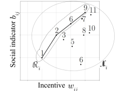
Figure 1: Alternative set $\mathcal{N}_{i}$ of individual $i$ and the subset $\mathcal{R}_{i}$ of LP-extremes.

We follow the Operations Research literature in the slight abuse of notation of denoting with $w_{i,j}$ the incentive to be provided to the $j$-th alternative in $\mathcal{R}_{i}$, where this is not ambiguous. With no loss of generality, we can assume the ordering

$$w_{i,1}<w_{i,2}<\dots<w_{i,r_{i}}$$ (11)

in the set $\mathcal{R}_{i}$, where $r_{i}$ is its cardinality. The default alternative of any individual is neither dominated nor LP-dominated, since it requires no incentive ($w_{i,j^{*}_{i}(0)}=0$). Therefore, the default alternative is the first alternative in the set $\mathcal{R}_{i}$ and $w_{i,1}=0$.

Definition 4.1 (Efficiency and incremental efficiency).

We define the efficiency of an alternative $j$ of individual $i$ as

$$e_{i,j}\equiv\frac{b_{i,j}-b_{i,j^{*}_{i}(0)}}{w_{i,j}},$$

i.e., the gain in social indicator that we can gain via a unit of incentive allocated to that alternative. We define the incremental social indicator $\tilde{b}_{i,j}$ and the incremental incentive $\tilde{w}_{i,j}$ required for each alternative $j\in\mathcal{R}_{i}$ as

$$\begin{array}[]{rl}\tilde{b}_{i,j}&\equiv b_{i,j}-b_{i,j-1}\\ \tilde{w}_{i,j}&\equiv w_{i,j}-w_{i,j-1}\end{array},\quad j=2,\dots,r_{i}.$$ (12)

The incremental efficiency is then defined as

$$\tilde{e}_{i,j}\equiv\tilde{b}_{i,j}/\tilde{w}_{i,j}.$$ (13)

The incremental efficiency $\tilde{e}_{i,j}$ can be interpreted as the increase in social welfare for each monetary unit spent, when individual $i$ shifts from alternative $j-1$ to alternative $j$.

4.2 Greedy Algorithm

We want to find a curve $\mathcal{C}_{Q}=\left\{(Y,B(Y))\>|\>Y\in[0,Q]\right\}$ that approximates the Maximum Social Welfare Curve $\mathcal{C}^{*}_{Q}$ (10), i.e., such that $B(Y)$ is close to $B^{*}(Y)$ for any value of budget $Y\geq 0$.

Very efficient algorithms, like the Dyer-Zemel algorithm (Kellerer et al. 2004, Section 11.2.1) are known to solve problem (9), i.e., to approximate the maximum social welfare for a fixed single value of budget $Q$. However, to apply them to the Maximum Social Welfare Curve problem, in which we want to find the maximum social welfare for a range of budget values $Y\in[0,Q]$, instead of just one, we would have to run those algorithms from scratch for every single value of budget. For this reason, we build our solutions upon a simpler greedy algorithm (Kellerer et al. 2004, Figure 11.2), which is less efficient to solve the Maximum Social Welfare problem (although still polynomial in time complexity), but easily extendable to also solve the Maximum Social Welfare Curve problem. The other advantage deriving from such choice is that this greedy algorithm has interesting properties that increase its practical application and economic interpretability, as discussed in Section 4.3.

The pseudocode of the algorithm is in Algorithm 1. The notation $[i,j]$ stands for ‘$j$-th alternative of individual $i$’. The idea of the algorithm is simple. First, the algorithm finds all the LP-extremes alternatives and sorts them by order of decreasing incremental efficiency. Then, at each iteration, the next pair of individual and alternative $[i^{\prime},j^{\prime}]$ with the highest incremental efficiency is picked (line 1). The alternative induced to $i^{\prime}$ is set to $j^{\prime}$ (line 1) and the budget is reduced by the amount of the incremental weight (equation (14)). An additional piece of the approximation of the social welfare curve is computed (equation (16)). The algorithm stops when the maximum budget $Q$ is depleted and it returns a policy $\mathbf{y}$, which is such that any individual $i$, for whom the algorithm selected an alternative $j\in\mathcal{R}_{i}$, effectively chooses this alternative $j$.

Input : Social indicators $\{b_{i,j}\}_{i,j}$, intrinsic utilities $\{V_{i,j}\}_{i,j}$, budget $Q$

1 Iteration index $k:=0$

2 $Y^{[k]}:=0$, Total incentive allocated so far.

3 ${B}^{[k]}:=0$, Social welfare obtained in the current allocation.

4 Compute the ordered set $\mathcal{R}_{i}$ of LP-extremes of each individual $i$.

5 Sort all the alternatives $[i,j]$ according to decreasing incremental efficiency $\tilde{e}_{i,j}$ and put them in a set $\mathcal{R}$.

6 Initialize the alternatives chosen by the individuals $\{x_{i,j}\}_{i,j}$ as follows

$$\left\{\begin{array}[]{ll}x_{i,1}=1,&\text{(default alternative)}\\ x_{i,j}=0,&\text{for any alternative }j>1\end{array}\right.$$

7 while $\mathcal{R}\neq\emptyset$ and $Y^{[k]}\leq Q$ do

8       Take $[i^{\prime},j^{\prime}]$, the next alternative with the highest incremental efficiency $\tilde{e}_{i^{\prime},j^{\prime}}$ from $\mathcal{R}$.

9       Add $[i^{\prime},j^{\prime}]$ to the solution, i.e.:

$$\mathcal{R} :=\mathcal{R}\setminus\{[i^{\prime},j^{\prime}]\},$$

$$Y^{[k+1]} :=Y^{[k]}+\tilde{w}_{i^{\prime},j^{\prime}}$$ (14)

$$\tilde{e}^{[k]} :=\tilde{e}_{i^{\prime},j^{\prime}}$$ (15)

$$B(Y) :={B}^{[k]}, \forall Y\in[Y^{[k]},Y^{[k+1]})$$ (16)

$${B}^{[k+1]} :={B}^{[k]}+\tilde{b}_{i^{\prime},j^{\prime}}$$

$$k :=k+1$$

10       Update the selected alternative for individual $i^{\prime}$, i.e.,

$$\left\{\begin{array}[]{rll}x_{i^{\prime},j^{\prime}}&=1,&\\ x_{i^{\prime},j}&=0,&\text{ for any other alternative }j\neq j^{\prime}\end{array}\right.$$

11 end while

Output :  Curve $\mathcal{C}_{Q}=\left\{(Y,B(Y))\>|\>Y\in[0,Q]\right\}$

Chosen alternatives $\{x_{i,j}\}_{i,j}$

Incentive policy $\mathbf{y}=\{y_{i,j}\}_{i,j}$, where $y_{i,j}=x_{i,j}\cdot w_{i,j}$

Split item $[s,t]:=[i^{\prime},j^{\prime}]$

Incremental efficiency of the split item $\tilde{e}_{s,t}$

Budget actually used $\widetilde{Q}:=Y^{[k-1]}$

Algorithm 1 Greedy algorithm for the Maximum Social Welfare and Maximum Social Welfare Curve problems.

Observe that the curve $\mathcal{C}_{Q}$ given as output by the algorithm is an approximation of the solution $\mathcal{C}^{*}_{Q}$ of the Maximum Social Welfare Curve Problem (Section 3.4). Moreover, given any maximum budget $Q$, the algorithm returns an approximation $B(Q)$ to the solution $B^{*}(Q)$ of the Maximum Social Welfare Problem (9). Note that, in order to achieve $B(Q)$, the policy issued by the algorithm does not spend the entire maximum budget $Q$, but only $\widetilde{Q}\leq Q$.

The algorithm also gives as output the incremental efficiency of the ‘split item’, denoted with $\tilde{e}_{s,t}$, useful to compute the optimality gap of the algorithm (Theorem 4.2 below). The name split item, which we borrow from Kellerer et al. (2004), reminds of the fact that, when we allocate the budget $Q$, we add to the solution all the LP-extreme alternatives, in decreasing order of incremental efficiency, up to $[s,t]$. In other words, such alternative $[s,t]$ splits the set $\mathcal{R}$ of all the LP-extremes in two parts: the first part consists of the alternatives we include in our solution, while we do not include the LP-extremes from the second part.

The distance to the optimum, in terms of social welfare, is bounded from above.

Theorem 4.2 (Upper bound).

Let us run Algorithm 1 with budget $Q$, and let $\widetilde{Q}$ be the budget actually used and $\tilde{e}_{s,t}$ be the incremental efficiency of the split item. The social welfare $B(Q)$ we obtain is boundedly close to the social welfare $B^{*}(Q)$ of any optimal personalized-incentive policy (Definition 3.11). In particular,

$$B^{*}(Q)-B(Q)\leq\tilde{e}_{s,t}\cdot(Q-\widetilde{Q}).$$ (17)

Corollary 4.3.

The curve $\mathcal{C}_{Q}$ obtained via Algorithm 1 is boundedly close to the Maximum Social Welfare Curve $\mathcal{C}^{*}_{Q}$ from equation (10) and the gap is given by Theorem 4.2.

The next corollary says that, for any budget $Q$, the curve $\mathcal{C}_{Q}$ returned by Algorithm 1 and the Maximum Social Welfare Curve $\mathcal{C}^{*}_{Q}$ ‘touch each other’. This ensures that the allocation computed by Algorithm 1 at every iteration is optimal. It is a direct consequence of Theorem 4.2.

Corollary 4.4.

The curve $\mathcal{C}_{Q}$ obtained via Algorithm 1 and the Maximum Social Welfare Curve $\mathcal{C}^{*}_{Q}$ from equation (10) are such that $B(Y^{[k]})=B^{*}(Y^{[k]})$ in all the values $Y^{[k]}$, $k=0,1,\dots$

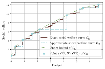
Figure 2: Distance between the social welfare curve $\mathcal{C}_{Q}$ computed by Algorithm 1, the maximum social welfare curve $\mathcal{C}^{*}_{Q}$ (Section 3.4) and the upper bound of Theorem 4.2. The stars represent the incentive spent $Y^{[k]}$ and social welfare $Y^{[k]}=B^{*}(Y^{[k]})$ at each iteration $k=1,\dots,8$ of the algorithm (line 9).

Figure 2 illustrates this property. The continuous curve represents the Maximum Social Welfare Curve $\mathcal{C}^{*}_{Q}$ and the dashed curve represents the curve $\mathcal{C}_{Q}$ obtained via Algorithm 1. These two curves are step-functions because of the discreteness of the problem. From Corollary 4.4, the curve $\mathcal{C}_{Q}$ intersects the curve $\mathcal{C}^{*}_{Q}$ at each iteration of the algorithm (represented by the stars). The dotted curve represents the upper bound of $\mathcal{C}^{*}_{Q}$, computed from Theorem 4.2.

4.3 Useful Properties for Large-Scale Applications

Our aim is to compute a personalized-incentive policy in large scenarios in a small amount of time. It is therefore crucial to show that our algorithm is computationally efficient.

Proposition 4.5.

The computational complexity of Algorithm 1 is $O(\sum_{i=1}^{m}|\mathcal{N}_{i}|\cdot\log|\mathcal{R}_{i}|+|\mathcal{R}|\cdot\log m)$, where $m$ is the number of individuals, $|\mathcal{N}_{i}|$ is the number of alternatives of individual $i$, $|\mathcal{R}_{i}|$ is the number of LP-extremes of individual $i$ and $|\mathcal{R}|\equiv\sum_{i=1}^{m}|\mathcal{R}_{i}|$.

Note that, since the alternatives of each individual are independent of the others, the sets $\mathcal{R}_{i}$ can be computed in parallel, thus reducing even further the computation time.

Despite our algorithm being computationally efficient, there might be cases in which it is desirable to stop it prematurely, without waiting for it to completely terminate. This can be the case when a personalized-incentive policy must be computed on-the-fly, within tight time-constraints. The following properties ensure that our algorithm is suitable to this situation, which eases its practical adoption.

Remark 2 (Anytime algorithm).

Algorithm 1 is anytime: if we stop it prematurely at any iteration $k$, we get a valid solution for the Maximum Social Welfare and the Maximum Social Welfare Curve problems, with budget $Q^{\prime}=Y^{[k]}$.

Remark 3 (Incremental use).

Another desirable property of Algorithm 1 is that we can build on a previously computed incentive allocation whenever new available budget becomes available, instead of recomputing the entire allocation from scratch. To explain this, let us suppose that we have a certain budget $Q$ and the algorithm returns the allocation $\{x_{i,j}\}_{i,j}$, spending the corresponding incentive amount $\widetilde{Q}$. Suppose now that the available budget increases to $Q^{\prime}>Q$. In this case, in order to exploit the new additional budget, we can simply resume the algorithm from its last iteration and continue up to the furthest iteration such that $Y^{[k+1]}\leq Q^{\prime}$. This is, per-se, a computational advantage with respect to algorithms that need to run from scratch every time new resources (budget) are available.

In order to describe the diminishing return property of Algorithm 1, we need the following definition.

Definition 4.6 (Incremental and overall efficiency).

The incremental efficiency provided by the algorithm at iteration $k$ is $\tilde{e}^{[k]}$, defined in equation (15). We define the overall efficiency of a personalized-incentive policy spending budget $Y$ and achieving social welfare $B$ as $e=B/Y$. We denote with $e^{[k]}$ the overall efficiency of the policy obtained by stopping Algorithm 1 at iteration $k$, i.e., $e^{[k]}=B^{[k]}/Y^{[k]}$.

The following proposition illustrates that, by spending more and more budget and allocating it as the algorithm dictates, we increase social welfare, but the marginal gain per unit of budget spent decreases.

Proposition 4.7 (Diminishing returns).

The incremental efficiency $\tilde{e}^{[k]}$ and the overall efficiency $\tilde{e}^{[k]}$ of the alternative added by Algorithm 1 at every iteration $k$ are both monotonically non-increasing.

The following corollary is a consequence of Proposition 4.7.

Corollary 4.8.

At any iteration $k$, we can compute an upper bound $B^{\text{ub}}\geq B(Q)$ to the social welfare we would get if we continue the algorithm until the end. Such an upper bound is $B^{\text{ub}}=B(Y^{[k]})+\tilde{e}^{[k]}\cdot(Q-Y^{[k]})$.

Therefore, if we notice that $B(Y^{[k]})$ is already sufficiently close to $B^{\text{ub}}$, then it is not worth continuing the algorithm, as we would not get much additional social welfare. In this case, we can safely stop the algorithm, without waiting for it to end, thus saving time.

In some cases, the regulator would be willing to maximize social welfare under the constraints that the overall inverse efficiency $e^{-1}$ is below a certain target. For instance, in Section 7.5 the regulator does not want to spend more than 100 euros per ton of CO₂ saved, which is considered to be the carbon price. In such cases, it is useful to observe that, thanks to Proposition 4.7, $(e^{[k]})^{-1}$ is non-decreasing. Therefore, the regulator could run the algorithm and stop at the iteration where $(e^{[k]})^{-1}$ goes above the target inverse efficiency.

We close this section with a definition that will be useful in Section 5.

Definition 4.9 (Maximum Step Size and Characteristic Incremental Efficiency).

Let us run Algorithm 1 with a certain budget $Q$ and record the values $Y^{[k]}$ calculated therein, as well as the incremental efficiency of the split item $\tilde{e}_{s,t}$. The maximum step size is defined as $\gamma_{Q}\equiv\max_{k=1,2,\dots}(Y^{[k]}-Y^{[k-1]})$. The characteristic incremental efficiency of budget $Q$ is defined as $\tilde{e}_{Q}\equiv\tilde{e}_{s,t}$.

The properties presented in this section have shown that the proposed Algorithm 1 is computationally efficient and able to return an allocation providing a welfare close to the optimum. Moreover, it has some features that make its adoption easier in practical large-scale scenarios.

5 Comparison with Other Policies

So far, we have considered that the regulator uses personalized incentives to increase social welfare. In particular, the policy proposed is such that the loss in individual utility, due to the shift to another alternative, is compensated exactly by the incentive. In this section, to frame our proposed personalized-incentive policy into a more general set of feasible policies, we generalize the formulation to include not only personalized incentives, but also enforcement policies, taxation, and non-personalized-incentive policies. In Section 5.1, we show that any optimal personalized-incentive policy (Definition 3.11) is optimal in this more general class of policies. In Section 5.2, we show that Algorithm 1 can be used to compute an enforcement policy and a proportional tax-subsidy policy, which are both boundedly close to the optimal general policy. We finally analytically show that non-personalized-incentive policies, like Tripod (Araldo et al. 2019), achieve by construction less social welfare than our personalized-incentive policy, and we provide a lower bound to this social welfare gap.

5.1 Optimality of Personalized-Incentives Policies among General Policies

We now consider a more general space of policies, including incentives, enforcement and taxation policies, and we define a criteria of optimality in this space. In order to do so, we need to define some new quantities.

The total loss in individual utility, of a policy $\mathbf{z}$, is

$$\Delta U(\mathbf{z})\equiv\sum^{m}_{i=1}\left(V_{i,j^{*}_{i}(0)}-U_{i,j^{*}_{i}(\mathbf{z})}(\mathbf{z})\right).$$ (18)

With a taxation policy, i.e., a policy $\mathbf{z}$ such that $z_{i,j}\leq 0$, $\forall i,j$, the loss in individual utility is non-negative, i.e., $\Delta U(\mathbf{z})\geq 0$. With an incentive policy, i.e., a policy $\mathbf{z}$ such that $z_{i,j}\geq 0$, $\forall i,j$, the loss in individual utility is non-positive, i.e., $\Delta U(\mathbf{z})\leq 0$. In particular, in any personalized-incentive policy obeying to Proposition 3.7, the individuals are perfectly compensated for their loss in utility, and thus $\Delta U(\mathbf{z})=0$, in accordance with Remark 1. Keeping everything else fixed, it is obvious that, the smaller $\Delta U$, the better.

The disutility, or cost, of a policy is measured by combining the loss in individual utilities and the expenses for the regulator, defined in equation (3).

Definition 5.1 (Disutility).

The disutility $\delta(\mathbf{z})$ of a policy $\mathbf{z}$ is defined as the expenses of the regulator $Y(\mathbf{z})$ plus the total loss in individual utilities $\Delta U(\mathbf{z})$, i.e.,

$$\delta(\mathbf{z})\equiv Y(\mathbf{z})+\Delta U(\mathbf{z}).$$ (19)

The following proposition shows that the disutility of a policy is always non-negative, which means that it is not possible that both the individuals increase their utility and the regulator collects revenues. It also shows that, if two policies imply the same alternatives chosen, then they have the same disutility.

Proposition 5.2.

Every policy $\mathbf{z}$ has a non-negative disutility that only depends on the alternative chosen by the individuals, rather than the actual incentive or taxation proposed. In particular:

$$\delta(\mathbf{z})=\sum_{i=1}^{m}\left(V_{i,j^{*}_{i}(0)}-V_{i,j^{*}_{i}(\mathbf{z})}\right)\geq 0$$

We can now define an optimal general policy, whose definition includes incentive, taxation and enforcement policies.

Definition 5.3 (Optimal General Policy).

An optimal general policy $\mathbf{z}$ with disutility threshold $Q\geq 0$ is the solution of the following problem:

$$\left\{\begin{array}[]{cl}\displaystyle\max_{\mathbf{z}}&B(\mathbf{z})\\ \text{s.t.}&\delta(\mathbf{z})\leq Q\\ \end{array}\right..$$ (20)

Note that, problem (20) is a generalization of (7). Indeed, we obtain the latter from the former by (i) constraining the policy to be a personalized-incentive policy, i.e., $z_{i,j}\geq 0,\forall i\in\mathcal{I},j\in\mathcal{N}_{i}$ and (ii) imposing no change in individual utility, i.e., $\Delta U(\mathbf{z})=0$.

The two next propositions characterize the optimal general policy. The first one implies that finding an optimal general policy is equivalent to finding a chosen-alternative set which maximizes social welfare, subject to a disutility constraint.

Proposition 5.4.

Let $\mathbf{z}$ be an optimal general policy with disutility threshold $Q$. Any other policy $\mathbf{z}^{\prime}$ inducing the same alternatives is also an optimal general policy, independent of the actual value of the single incentives or taxes proposed.

The following proposition shows that the personalized-incentive policy, considered previously, is still relevant in this more general framework. The proposition states that, for any disutility threshold $Q$, it is possible to find an optimal policy which is a personalized-incentive policy.

Proposition 5.5.

For any $Q\geq 0$, any optimal personalized-incentive policy $\mathbf{y}$ with budget $Q$ (Definition 3.11) is also an optimal general policy with disutility threshold $Q$ (Definition 5.3).

The following corollary states that the social welfare bound for personalized-incentive policies (Theorem 4.2) is equivalent for general policies.

Corollary 5.6.

Let us run Algorithm 1 with budget $Q$ to construct a personalized-incentive policy. The social welfare $B(Q)$ we obtain is boundedly close to the optimum $B^{*}(Q)$, obtainable with an optimal general policy with disutiliy threshold $Q$. In particular,

$$B^{*}(Q)-B(Q)\leq\tilde{e}_{s,t}\cdot(Q-\widetilde{Q}).$$

5.2 Computing Optimal Enforcement and Proportional Tax-Subsidy Policy

In this section, we show how Algorithm 1 can be used, in conjunction with Propositions 5.5 and Corollary 5.6, to compute an enforcement policy and a proportional tax-subsidy policy boundedly close to the optimum.

We provide a numerical comparison between these policies in Section 7.6.

5.2.1 Enforcement Policy

With enforcement policies, the regulator constrains the individuals to choose an alternative among a subset of their choice set. In the most extreme case, the individuals can choose only one alternative.

Let $\mathbf{y}$ be the personalized-incentive policy returned by Algorithm 1, for a budget $Q$. Consider now a policy $\mathbf{z}$ enforcing the individual to choose the same alternative that they would choose under the policy $\mathbf{y}$, i.e.,

$$\left\{\begin{array}[]{ll}z_{i,j}=0,&\text{if}\>j=j^{*}_{i}(\mathbf{y})\\ z_{i,j}=-\infty,&\text{otherwise}\\ \end{array}\right.,\quad\forall i,j.$$

Proposition 5.7.

The enforcement policy $\mathbf{z}$ constructed above is boundedly close to an optimal general policy with disutility constraint $Q$. The bound is the same as Corollary 5.6.

5.2.2 Proportional Tax-Subsidy Policy

We consider here policies $\mathbf{z}$ for which the monetary transfers are proportional to the social indicator of the alternatives, that is

$$z_{i,j}=\tau\cdot(b_{i,j}-A_{i}),\quad\forall i,j,$$ (21)

where $\tau>0$ is the tax-subsidy level and $A_{i}\in\mathbb{R}$ is an individual-specific baseline social-indicator, set by the regulator. We call these policies proportional tax-subsidy policies. Observe that, for any individual $i$, her alternatives $j\in\mathcal{N}_{i}$ such that the social indicator is below the baseline are taxed (i.e., $b_{i,j}<A_{i}\Rightarrow z_{i,j}<0$). Conversely, alternatives $j\in\mathcal{N}_{i}$ having social indicator above the baseline are subsidized (i.e., $b_{i,j}>A_{i}\Rightarrow z_{i,j}>0$). The baseline social-indicators $A_{i}$ can vary from individual to individual. However, we impose that the tax-subsidy level $\tau$ is the same for everyone. In this sense, we consider that these policies are not personalized.

Observe from equations (1) and (21) that, considering any individual $i$, if we vary the baseline $A_{i}$ the variation of the utility $U_{i,j}$ is the same for all alternatives $j\in\mathcal{N}_{i}$. Hence, the value of $A_{i}$ does not impact the choice of $i$. It simply represents a monetary transfer between the individual and the regulator. More precisely, setting low $A_{i}$ favours transfers from the regulator to individuals, thus increasing individual utilities, to the detriment of the regulator. On the other hand, setting high $A_{i}$, favours the revenue of the regulator, to the detriment of the utility of the individuals.

Note that, if $b_{i,j}$ represents a negative externality (as in Section 7), then the tax-subsidy policy defined above is equivalent to a Pigouvian tax if $\tau$ is set to be equal to the external marginal cost of the externalities and $A_{i}=0$. For instance, it has been estimated (Quinet et al. 2009), that the social cost of 1 ton of CO₂ is 100 euros. Then, if $b_{i,j}$ represents CO₂ emissions (in tons), the Pigouvian tax would be a proportional tax-subsidy policy with $\tau=100$ euros.

The following theorem shows that we can use Algorithm 1 to compute a proportional tax-subsidy policy that is boundedly close to the theoretical optimum.

Theorem 5.8.

We can construct a proportional tax-subsidy $\mathbf{z}$ under a certain disutility threshold $Q$ as follows. Run Algorithm 1 with budget constraint $Q$ and let $\tilde{e}_{s,t}$ be the incremental efficiency of the split item given as output.

The proportional tax-subsidy policy $\mathbf{z}$, defined as in equation (21), with tax-subsidy level

$$\tau=1/\tilde{e}_{s,t}$$ (22)

achieves a social welfare that is boundedly close to the optimal general policy with disutility threshold $Q$. The bound is the same as Corollary 5.6.

5.2.3 Comparison with Proportional-Incentive Policy and Tripod

A proportional-incentive policy $\mathbf{z}$ is a proportional tax-subsidy policy, as in (21) where only subsidies and not taxes are distributed, i.e.

$$A_{i}\leq b_{i,j},\quad\forall i\in\mathcal{I},j\in\mathcal{N}_{i}.$$ (23)

An example of proportional-incentive policy is Tripod (Araldo et al. 2019).

In this section we show that proportional-incentive policies are inefficient incentive policies, in the sense that, to achieve a certain social welfare level, they spend more incentives than needed. We call ‘inefficiency gap’ this additional incentive spent and we compute a lower bound for it in the following proposition.

Proposition 5.9.

Consider a proportional-incentive policy $\mathbf{z}$ as before. There always exists a personalized-incentive policy $\mathbf{y}$ that is able to achieve at least the same social welfare and provides the following savings in the amount of incentive spent:

$$Y(\mathbf{z})-Y(\mathbf{y})\geq\frac{1}{\tau}\cdot\sum_{i\in\mathcal{I}}\left(V_{i,j^{*}_{i}(\mathbf{z})}-V_{i,j^{*}_{i}(0)}\right)\cdot\Delta e_{i,j^{*}_{i}(\mathbf{z})}\equiv L(\mathbf{z})$$

where $\Delta e_{i,j}\equiv e_{i,j}-1/\tau$ is defined as efficiency loss, $\forall i\in\mathcal{I},j\in\mathcal{N}_{i}$. The quantity $L(\mathbf{z})$ defined above is a lower bound for the inefficiency gap.

Note that the efficiency loss quantifies the fact that proportional-incentive policies are not able to exploit the inherent efficiency $e_{i,j}$ (see Definition 4.1) of the incentivized alternative. Indeed, instead of using such an alternative-dependent efficiency, they use a single value $1/\tau$.

We compute in the following proposition a lower bound on the suboptimality gap of proportional-incentive policies.

Proposition 5.10.

Let us consider a proportional-incentive policy $\mathbf{z}$, achieving a social welfare $B(\mathbf{z})$ and spending an incentive amount $Y(\mathbf{z})$. Let us denote with $B^{*}(Y(\mathbf{z}))$ the maximum social welfare achievable by an optimal personalized-incentive policy with that incentive amount. The following lower bound holds on the suboptimality gap:

$$B^{*}(Y(\mathbf{z}))-B(\mathbf{z})\geq\max\left\{0,\tilde{e}_{Y(\mathbf{z})}\cdot\left(L(\mathbf{z})-2\gamma_{Y(\mathbf{z})}\right)\right\}$$

where $\gamma_{Y(\mathbf{z})}$ and $\tilde{e}_{Y(\mathbf{z})}$ are the maximum step size and the characteristic incremental efficiency, as defined in Definition 4.9.

We now draw an interesting parallel with Tripod, a proportional incentive policy described in Araldo et al. (2019). In Tripod, social welfare is represented, in particular, by energy reduction. While our formulation is general and can encompass any type of social welfare (provided that the assumptions of Section 3 are valid) in our case study (Section 7) we consider CO₂ reduction. In both our case study and Tripod, individuals are travellers and alternatives are modal choices. An important aspect of Tripod is that it is dynamic, i.e., time is slotted and, in each time slot, the incentives for the individuals happening to depart in that time slot are calculated. With the Tripod policy, that we denote $\mathbf{z}^{\text{Tr}}$, the incentives proposed to individuals are proportional to the gain in the social indicator with respect to the default alternative, i.e.

$$z_{i,j}^{\text{Tr}}=(b_{i,j}-b_{i,j^{*}_{i}(0)})/\text{TEE}_{t}$$

where the constant $\text{TEE}_{t}$ is called Token Energy Efficiency and is fixed by the regulator in every time slot $t$. In Tripod, the incentives are distributed to individuals under a First-Come First-Served discipline, until a certain budget is depleted. Therefore, out of the entire population $\mathcal{I}_{t}$ of individuals departing at time slot $t$ only a subset $\mathcal{I}_{t}^{\text{Tr}}$ actually receive an incentive. In Araldo et al. (2019), the value of $\text{TEE}_{t}$ is fixed empirically, with a grid search, trying several values of $\text{TEE}_{t}$ in simulation and choosing the one with maximum social welfare. The calculation is based on a Model-Predictive Control (MPC) setting, where at every time slot the value of $\text{TEE}_{t}$ is calculated taking into account not only the current time slot, but also a prediction of the system state (congestion, individual arrival) in the subsequent time-slots, which are called optimization horizon. Note that the MPC setting of Tripod allows to take into account the impact of the incentive policies on congestion, which we instead neglect, based on Assumptions 3.2 and 3.3. Therefore, for adopting our policy to a real scenario, care should be taken in checking that such Assumptions are reasonable, as we do in our case study.

Within our framework, Tripod can be defined as a proportional-incentive policy, with $\tau=1/\text{TEE}_{t}$ and $A_{i}=b_{i,j^{*}_{i}(0)}$, applied to population $\mathcal{I}_{t}^{\text{Tr}}$.

As a consequence of Proposition 5.9, Tripod is an inefficient incentive policy, under the assumptions of Section 3.1. In Corollary 5.11, we lower-bound the additional incentive spent with respect to the theoretical best incentive policy.

Corollary 5.11.

For any Tripod incentive policy $\mathbf{z}^{\text{Tr}}$, there always exists a personalized-incentive policy $\mathbf{z}$ that is able to achieve at least the same social welfare while spending less incentives. The saving in the incentives is:

$$Y(\mathbf{z}^{\text{Tr}})-Y(\mathbf{z})\geq\sum_{t}\text{TEE}_{t}\cdot\sum_{i\in\mathcal{I}_{t}^{\text{Tr}}}\left(V_{i,j^{*}_{i}(\mathbf{z}^{\text{Tr}})}-V_{i,j^{*}_{i}(0)}\right)\cdot\Delta e_{i,j^{*}_{i}(\mathbf{z}^{\text{Tr}})}$$

where $\Delta e_{i,j}\equiv e_{i,j}-\text{TEE}_{t}$ is defined as efficiency loss, $\forall i\in\mathcal{I}_{t}^{\text{Tr}},j\in\mathcal{N}_{i}$ and $\mathcal{I}_{t}^{\text{Tr}}$ is the set of individuals getting incentives in Tripod in time-slot $t$.

Corollary 5.11 shows that Tripod is far from minimizing the incentives needed to obtain a certain social welfare, while the policy issued by Algorithm 1 is generally close to using minimal incentives. This is confirmed by our numerical results in Section 7.6. An interpretation of the inefficiency suffered by Tripod follows.

Remark 4.

Tripod uses a single value $\text{TEE}_{t}=1/\tau$ to compute incentives for all alternatives $j$ of all users $i\in\mathcal{I}_{t}$ and gets $1/\text{TEE}_{t}$ additional units of social welfare per additional unit of incentive spent. The only incentivized alternatives are the ones for which $e_{i,j}\geq\text{TEE}_{t}$ (otherwise the proposed incentive would not be accepted by the individual). In other words, Tripod gets always an efficiency (unit of social welfare improvement over unit of incentive spend) that is lower than the intrinsic efficiency of the incentivized alternatives. By contrast, our personalized policy always entirely exploits the intrinsic efficiency of the incentivized alternatives.

Since Tripod is a proportional-incentive policy, the same lower bound on the suboptimality gap as in Proposition 5.10 also holds, which we do not write for the sake of space.

6 Imperfect Information

The assumption that the regulator knows perfectly the utility of the individuals may seem restrictive. In this section, we show that the algorithm is still relevant when the utility is imperfectly known. From discrete-choice theory (Anderson, de Palma, and Thisse 1992), we assume that intrinsic utility of alternative $j$ of individual $i$ is composed of a deterministic part $\hat{V}_{i,j}$ and a random part $\epsilon_{i,j}$:

$$V_{i,j}=\hat{V}_{i,j}+\epsilon_{i,j}.$$

We assume that the regulator knows the deterministic part $\hat{V}_{i,j}$ of the utility but not the random part $\epsilon_{i,j}$.

Under this assumption, the regulator cannot compute the minimum incentive amount needed to induce individual $i$ to shift from her default alternative $j^{*}_{i}(0)$ to another alternative $j$, using directly equation (6). A heuristic solution would be to set the incentive amount equal to the expectation of the utility difference between the two alternatives, given that $j^{*}_{i}(0)$ is the default alternative chosen when there is no incentive. In this case, the incentives $\{y_{i,j}\}_{j\in\mathcal{N}_{i}}$ proposed by the regulator to individual $i$, to convince her to shift to alternative $j$, are such that $y_{i,{j^{\prime}}}=0$, for any ${j^{\prime}}\neq j$, and

$$y_{i,j}=\mathbb{E}(V_{i,j^{*}_{i}(0)}-V_{i,j}|V_{i,j^{*}_{i}(0)}>V_{i,j})=\hat{y}_{i,j}+\mathbb{E}(\epsilon_{i,j^{*}_{i}(0)}-\epsilon_{i,j}|\epsilon_{i,j^{*}_{i}(0)}-\epsilon_{i,j}>-\hat{y}_{i,j}),$$ (24)

where $\hat{y}_{i,j}=\hat{V}_{i,j^{*}_{i}(0)}-\hat{V}_{i,j}$ is the difference in the deterministic part of the utility, known to the regulator.

Given an individual $i$ and an alternative $j\in\mathcal{N}_{i}$, if the regulator proposes the incentive $y_{i,j}$, as defined by equation (24), then individual $i$ has a positive probability to refuse the incentive. Hence, the expenses of the regulator may be smaller than the total incentive amount proposed.

Algorithm 1 can be used to compute a personalized-incentive policy under imperfect information, by defining new weights

$$w_{i,j}=\mathbb{E}(V_{i,j^{*}_{i}(0)}-V_{i,j}|V_{i,j^{*}_{i}(0)}>V_{i,j}).$$

At each iteration of the algorithm, the regulator proposes the incentive $w_{i^{\prime},j^{\prime}}$ to individual $i^{\prime}$ for alternative $j^{\prime}$, where $[i^{\prime},j^{\prime}]$ is the pair of individual and alternative selected by the algorithm. The regulator observes the response of the individual to the incentive. If the individual accepts the incentive, it decreases the budget by the incentive amount. The regulator keeps proposing incentives one by one until his budget is depleted.

Note that, if an individual $i$ accepts an incentive $y_{i,j}$ for alternative $j\in\mathcal{N}_{i}$, the regulator can still propose her, later, an incentive $y_{i,{j^{\prime}}}$ for another alternative ${j^{\prime}}\in\mathcal{N}_{i}$. If the individual refuses the second incentive $y_{i,{j^{\prime}}}$, she still receives the first incentive $y_{i,j}$.

In Section 7.7, we apply the policy presented above to our case study and compare it to the case with perfect information, assuming that random terms are Gumbel-distributed. The following proposition gives the exact expression of the incentives (24), in case of Gumbel-distributed random terms.

Proposition 6.1.

Let us assume that the random terms are i.i.d. and follow a Gumbel distribution with scale parameter $\mu$ (i.e., $\epsilon_{i,j}/\mu$ follows a standard Gumbel distribution). Then, the incentive amount from equation (24) can be written as

$$y_{i,j}=\mu\frac{1+e^{\hat{y}_{i,j}/\mu}}{e^{\hat{y}_{i,j}/\mu}}\ln\left(1+e^{\hat{y}_{i,j}/\mu}\right)\geq 0.$$

7 Numerical Results in an Application to Mode Choice

In this section, we simulate an application of our personalized incentive policy to a scenario related to mode choice of individuals commuting to their workplace. We consider a regulator willing to employ a limited monetary budget in order to promote eco-friendly modes of transportation. The goal of the regulator is to reduce CO₂ emissions. We compute the reduction in CO₂ emissions achieved via the personalized-incentive policy of Algorithm 1 and compare it with enforcement, proportional taxation and non-personalized-incentive policies.

Our approach is as follows. After describing the census data used to build the simulation scenario (Section 7.1), we estimate a Multinomial Logit model for mode choice (Section 7.2). Then, using the previous estimates, we simulate the utility of a home-work trip for a group of individuals, for all the modes of transportation considered (Section 7.3). We then approximate the CO₂ emissions for these same trips (Section 7.4) and approximate the optimal personalized-incentive policy using Algorithm 1 (Section 7.5). We then study the modal shifts induced by such policy and the gain in CO₂ emissions achieved. We conclude the numerical results by comparing our personalized incentive policy with other policies (enforcement, taxation, flat incentives – Section 7.6) and by evaluating its performance in case of imperfect information (Section 7.7).

7.1 Data

We use census data from the French statistics institute INSEE, regarding households surveyed between 2015 and 2019. We restrict the dataset to households whose home and workplace are in the Rhône department, which includes Lyon and its suburbs (about $222\,000$ households in total). Observed variables include city- or district-level home and work location, main mode of transportation used for commuting, and some socio-demographic variables. The modes of transportation are divided in five categories: car, public transit, walking, cycling and motorcycle. Appendix C provides a detailed description of the data.

7.2 Multinomial Logit Model

Using the census data, we estimate a Multinomial Logit model for the mode choice of the individuals. We consider five exogenous variables specific to the individual (age, sex, number of cars owned per employee in the household and professional occupation) and one exogenous variable which is specific to both the mode of transportation and the individual (travel time). The number of cars owned is supposed to only impact the utility of commuting by car. Following Inoa, Picard, and de Palma (2015), we also include interaction variables between travel time and socio-demographic variables. Details on how travel time is computed are provided on Appendix D. To estimate the utility of the round trip to work, travel times are doubled (we assume that the modes of transportation for the trip back and forth are the same).

Note that public transit is excluded from the choice set of the individuals whose commute to work cannot be performed by public transit ($\simeq$$16\,000$ individuals, see Appendix D for more details).

The four other modes of transportation (car, walking, cycling and motorcycle) are assumed to be in the choice set of all the individuals. This is a strong assumption. A regulator willing to deploy the personalized-incentive policy in practice could improve the precision of the model by using individual-specific data for vehicle ownership in order to remove some modes of transportation from the choice set of an individual, if she does not own the corresponding vehicle.

Table 2 provides the results of the Multinomial Logit model, estimated with the R package mlogit. The most frequent categories are used as reference category (car for the mode of transportation, man for the sex and employee for the occupation).

Table 2: Multinomial Logit model of mode choice

	(1)	(2)	(3)	(4)	(5)
	car	public_transit	walking	cycling	motorcycle
constant		2.7709***	2.8659***	1.1340***	-0.7284***
		(0.0395)	(0.0488)	(0.0509)	(0.0773)
age		-0.0150***	-0.0026***	-0.0139***	-0.0019
		(0.0008)	(0.0009)	(0.0010)	(0.0015)
woman		0.5349***	0.4361***	-0.3882***	-1.6909***
		(0.0194)	(0.0248)	(0.0242)	(0.0527)
car_per_indiv	1.2138***
	(0.0161)
car_per_indiv$>$0	1.5604***
	(0.0245)
occupation: farmer		-3.9054***	-1.0434***	-2.3653***	-0.8798**
		(0.4140)	(0.2012)	(0.5073)	(0.4400)
occupation: artisan		-1.7023***	-1.2153***	-0.7848***	-0.2261***
		(0.0525)	(0.0566)	(0.0651)	(0.0841)
occupation: executive		0.1522***	0.2031***	1.1710***	0.2986***
		(0.0255)	(0.0327)	(0.0337)	(0.0575)
occupation: intermediate		-0.2283***	-0.1447***	0.4259***	-0.0060
		(0.0242)	(0.0311)	(0.0349)	(0.0584)
occupation: blue-collar		-0.7579***	-0.9691***	-0.4808***	-0.0259
		(0.0318)	(0.0413)	(0.0467)	(0.0616)
travel_time	-1.6281***	-1.1746***	-2.1032***	-2.8474***	-3.2075***
	(0.0530)	(0.0480)	(0.0492)	(0.0581)	(0.0968)
travel_time $\times$ age	-0.0026**
	(0.0010)
travel_time $\times$ woman	-0.1134***
	(0.0266)
travel_time $\times$ occupation: farmer	1.1027***
	(0.3621)
travel_time $\times$ occupation: artisan	-0.0763
	(0.0918)
travel_time $\times$ occupation: executive	-0.3671***
	(0.0354)
travel_time $\times$ occupation: intermediate	-0.1986***
	(0.0330)
travel_time $\times$ occupation: blue-collar	0.2623***
	(0.0403)
Reference category is male employee
Travel time is expressed in hours
Standard errors are reported in parentheses
*** p$<$0.01, ** p$<$0.05, * p$<$0.1

The results are consistent with the literature on commute mode choice. For example, we find that being young and male increases the probability to commute by cycling, consistently with the literature review of cycling mode choice from Muñoz, Monzon, and Daziano (2016). We also find that the coefficient of travel time is larger for public transit than for car which suggests that the value of time for commutes by public transit is slightly smaller than for commutes by car. This is coherent with the meta-analysis on the value of travel-time in France from Wardman et al. (2012).

7.3 Simulating Utilities

We consider a regulator whose goal is to reduce the CO₂ emissions due to commute trips, by distributing incentives to the population described in the data (about $222\,000$ individuals).

To apply Algorithm 1, the regulator needs to know the utility and the CO₂ emissions of each individual, for each mode of transportation. We describe in this subsection how we estimate them. Note that our estimations are individual specific.

Remark 5.

Recall that Assumption 3.2 implies that the utility of an individual when commuting by car or public transit does not depend on how many other individuals commute by car or by public transit. Such an assumption is reasonable when the congestion on the road and transit occupation rate are approximately exogenous, i.e., they do not depend on the incentive policy. This approximation is legitimate if the number of modal shifts induced by the policy is low, so that their impact on congestion and occupation is negligible. A posteriori, we check that this latter assumption is verified in our case, since less than $1.60$% of individuals shifted mode due to the personalized-incentive policy.

Following the Multinomial Logit theory, we assume that utility of alternative $j$ of individual $i$ is composed of a deterministic part $\hat{V}_{i,j}$ and a random part $\epsilon_{i,j}$:

$$V_{i,j}=\hat{V}_{i,j}+\epsilon_{i,j}.$$ (25)

The deterministic part of the utility can be computed using the estimates from Table 2. As for the random part, we simulate random draws from a random variable with standard Gumbel distribution (see Appendix E). In accordance with Assumption 3.4, the regulator is assumed to know perfectly both the estimates and the draws and thus the utilities. We relax this assumption in Section 7.7, where we provide results where the random draws are unknown to the regulator.

To normalize the utility in monetary units, we compare the value of travel time by car from our regression (expressed in utility units) with the value of travel time by car in France from the literature (expressed in euros). We compute the value of travel time by taking the opposite of the average marginal effect on utility of increasing the travel time of the individuals by one hour. We find an average value of time of $1.88$ utility units per hour.

Previous studies (Wardman et al. 2012) have shown that the value of travel time, for car commuters, in France, is about $9.17$ euros per hour. This would imply that, in our estimates, one utility unit corresponds to $\mu=9.17/1.88=4.88$ euros. In the following, we assume that the utility is normalized in monetary units, i.e., the values in equation (25) are multiplied by $\mu$. Note that it implies that the random variables $\epsilon_{i,j}$ follows a Gumbel distribution with scale parameter $\mu$.

7.4 Computing the Social Indicator

The regulator wants to reduce greenhouse gas emissions. The social indicator associated to the mode of transportation $j$ of individual $i$ is the reduction in CO₂ equivalent of greenhouse gas emissions generated during the trip of $i$ performed with mode $j$, with respect to the emissions of the default mode. To compute CO₂ emissions for each individual and each mode of transportation, we take the distance of the fastest path between the individual’s home and workplace and we multiply this distance with the CO₂ emissions equivalent per kilometre for the mode of transportation, using open-sourced data from the French agency ADEME (Agence de l’Environnement et de la Maîtrise de l’Énergie).

For car, we use the CO₂ emissions of a passenger car with average motorization ($0.193$ kilogram of CO₂ per kilometre). That is, we assume that the CO₂ emissions per kilometre are the same for everyone. We pinpoint that this assumption may lead to some imprecision in the calculation of the actual CO₂ reduction. The application could be improved by using detailed data on the characteristics of the vehicle used by each individual.

For Assumption 3.3 to be valid, CO₂ emissions due to the commuting trip of an individual must be independent from the mode of transportation chosen by the other commuters. For the same argument of Remark 5, we can claim that this approximately holds true in the scenario.

As Chester, Horvath, and Madanat (2010), we adopt a disaggregated view of CO₂ emissions from public transit. We consider that the overall CO₂ generated by transit vehicles is shared among all travellers making trips within transit, proportionally to the kilometres travelled. In other words, each trip on transit produces a quantity of CO₂ emissions equal to the number of kilometres travelled multiplied by the average CO₂ emissions per kilometre per passenger, assuming average and constant occupancy rate. Observe that it is reasonable to assume an average occupancy rate that is constant over time from the argument of Remark 5. The average CO₂ emissions per kilometre per passenger vary according to the mode of transportation used (e.g., bus, tramway or metro). The mode of transportation taken for the fastest path are used to compute CO₂ emissions. For multi-modal public-transit trips (e.g., bus then tramway), the CO₂ emissions are computed according to the distance travelled by each mode of transportation.

CO₂ emissions for walking and cycling trips are set to zero. Hence, for each individual, the two alternatives corresponding to walking and cycling differ only in the intrinsic utility. As a consequence, the alternative with smaller intrinsic utility can be neglected, thanks to Proposition 3.9.

Table 3: Our calculations of CO₂ emissions in the Rhône department.

Daily CO2 emissions (all home-work and work-home trips)	$595.26$ tons of CO2
Total CO2 emissions in one year (200 working days)	$119\,050$ tons of CO2
Average yearly individual CO2 emissions	0.54 tons of CO2

Recall that Assumption 3.4 implies that the regulator knows perfectly the CO₂ emissions of the trips. This is more realistic than for utility. In any case, measurement errors for CO₂ emissions are not as worrying as measurement errors for utility as we can assume that, if such errors are unbiased, they cancel out. We will observe in Section 7.7 that the errors are much more severe when utilities are imperfectly known, as some individuals might reject the incentives, which leads to a suboptimal allocation.

Under the previous assumptions, we calculate the CO₂ emissions reported in Table 3, which results in 0.54 ton of CO₂ yearly per individual in the Rhône department. This number is close to the publicly known estimation for the entire France: in 2007, the average French worker emitted 0.64 ton per year because of his/her home-work trips (Levy and Le Jeannic 2011).

7.5 Calculation of the Personalized-Incentive Policy

We consider a large-scale scenario with more than 200 thousands individuals and over 1 million alternatives (Appendix C). We consider a policy in which the regulator proposes, each day, incentives to the individuals before their home-work trip. The incentives are given conditional on the mode of transportation chosen for the round trip to work, thus the social indicator of an alternative is the reduction in CO₂ emissions for the trip back and forth, with respect to the default alternative. The budget represents the daily amount available to the regulator for incentives.

First, we run Algorithm 1 with a daily budget of $3000$ euros and we plot the maximum social welfare curve (see Figure 3). The maximum social welfare curve is an increasing step function (steps are small and thus not visible). Consistently with Proposition 4.7, the slope of each step is non-increasing, which gives the curve a concave curvature.

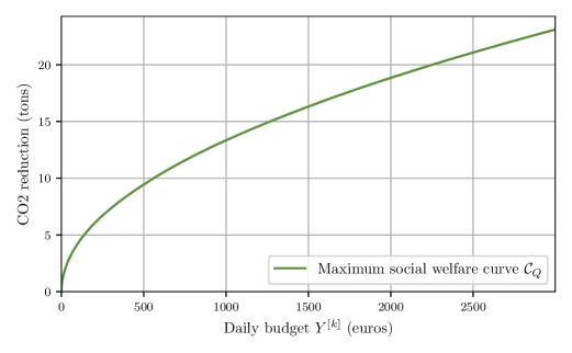
Figure 3: Maximum social welfare curve, up to a daily budget of 3000 euros. Note: The social welfare corresponds to the reduction in CO₂ emissions due to the personalized-incentive policy.

Quinet et al. (2009) predict that the carbon price in France would be of 100 euros per ton of CO₂ in 2030. It is thus reasonable to assume the regulator is interested in finding an incentive policy such that, for every 100 euros spent in incentives, pollution is reduced by at least a ton of CO₂. To this aim, the regulator can observe the curves of Figure 4, which plots the inverse of the incremental and overall efficiency (the $\tilde{e}^{[k]}$ and $e^{[k]}$ of Definition 4.6), with respect to the budget $Y^{[k]}$ allocated by the algorithm at each iteration $k$. Thanks to Proposition 4.7, $1/e^{[k]}$ and $1/\tilde{e}^{[k]}$ increase with $Y^{[k]}$, as we proceed with the iterations of the algorithm. Thanks to this monotonicity, the regulator can apply one of the following two criteria to fix the budget to invest. It could run Algorithm 4 and stop it when $1/e^{[k]}$ equals 100 euros per ton of CO₂. Alternatively, it can stop the Algorithm when $1/\tilde{e}^{[k]}$ equals 100 euros per ton of CO₂. From Figure 4, we observe that with the first criterion the regulator would need to invest about 1800 euros per day, and about 500 euros with the second criterion. In our opinion, both criteria would make sense, and the preference over one of them is a political choice.

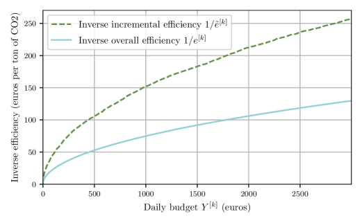
Figure 4: Cost of the policy in euros per ton of CO₂ prevented as a function of the daily budget.

We now set the budget of the regulator to $Q=$1800$$ euros. Running Algorithm 1 with this budget required about $3500$ iterations and took about 6 seconds (with Python, on a computer with an Intel i5-8350U 1.7GHz and 24GB of memory). The algorithm allocates practically all the budget ($1798.59$ euros). We find that $1.57$% of individuals received incentives and changed transportation mode, which results in a reduction of CO₂ emission by $18$ tons of CO₂ per day ($3.00\text{\,}\%$ of total CO₂ emissions). Thus, this policy would cost on average $100.61$ euros for each ton of CO₂ prevented.

Despite the small incentives, the reduction in CO₂ emissions is considerable. Indeed, among the individuals who received incentives, the average amount of incentives is $0.52$ euros per individual, for an average daily reduction in CO₂ emissions of $5$ kilograms. Recall that alternatives providing a large reduction in CO₂, while requiring small incentive, have a high efficiency. Hence, the algorithm selects first shifts achievable with a small incentive, i.e., where the individual is almost indifferent between the two alternatives, which however have a large difference in CO₂. Figure 5 shows the distribution of the incentive amount and the CO₂ reduction for the incentivized individuals. For most incentives, the amount proposed to individuals is below $1$ euro (incentives with a larger amount are not efficient enough, unless the CO₂ reduction is very high).

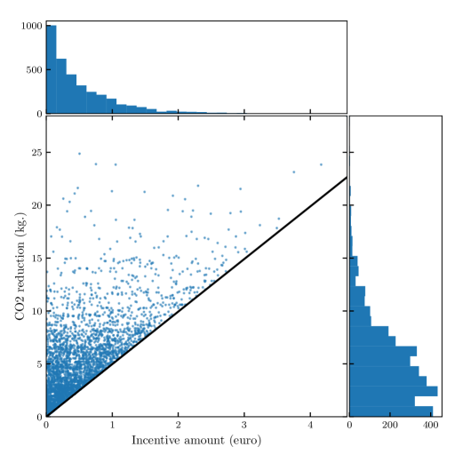
Figure 5: Distribution of incentive amount and CO₂ reduction for the incentives given in one day with budget $Q=1800$ euros.
The slope of the black line represents the incremental efficiency of the split item returned by the algorithm, $\tilde{e}_{s,t}=$5$$ tons of CO₂ / euro. Note that all points are above the line because their incremental efficiency is larger. The histogram above represents the distribution of the incentive amounts. The histogram on the right represents the distribution of the CO₂ reduction for the incentives.

Figure 6 compares mode share before and after the policy. Most individuals who received incentives are individuals who commuted by car and were induced to commute by public transit ($1.2$% of all individuals, $74$% of individuals who received incentives). The share of individuals commuting by car decreased by 2.4%, while public transit ridership increased by $4$%.

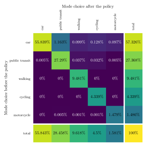
Figure 6: Evolution of mode share before and after the policy. $1.163\text{\,}\%$ of individuals were given incentives to shift from car to public transit, $27.29\text{\,}\%$ of individuals commuted by public transit before the policy and were not induced to shift.

We now compute a bound of the optimality gap, i.e., the maximum additional CO₂ savings we would achieve if we could use a theoretical optimal policy instead of resorting to Algorithm 1. To do so, we apply Theorem 4.2. Since the incremental efficiency of the split item returned by the algorithm is $\tilde{e}_{s,t}\simeq 5$ kilograms of CO₂ per euro and the unused budget is $Q-\widetilde{Q}=1.41$ euros, an optimal policy would reduce just $5\cdot 1.41\simeq 7$ kilograms more than Algorithm 1, which is negligible compared to the total CO₂ emissions reduction of $18$ tons provided overall.

7.6 Comparison with Other Policies

In Section 7.5, we evaluated the performance of the personalized incentive policy calculated by Algorithm 1, which we denote with $\mathbf{y}$. We now compare it with three other policies from Section 5.2: an enforcement policy, a proportional taxation system and the Tripod incentive system from Araldo et al. (2019).

Aggregate results for these policies are provided in Table 4. The policies are defined so that they induce the same choices for the individuals, using results from Section 3. Therefore, they provide the same reduction in CO₂ emissions and, from Proposition 5.2, they have the same disutility. However, they differ in their cost for the regulator and the variation in individual utilities implied. It should be noted that the best policy to implement depends on social, political or juridical constraints.

In these results, we fix the disutility threshold to $1798.59$ euros, which corresponds to the incentive $\widetilde{Q}$ actually spent by Algorithm 1 when we set the budget to $Q=1800$ euros. This means that if we run the algorithm setting a budget of $1798.59$ euros, it spends it all and, thanks to Corollary 5.6, the resulting policy is optimal under a budget constraint of $1798.59$ euros.

Table 4: Summary of policies.

Policy $\mathbf{z}$	Expenses (euros)	Ind. utility (euros)	Disutility (euros)	CO2 reduction (tons)
	$Y(\mathbf{z})$	$\Delta U(\mathbf{z})$	$\delta(\mathbf{z})$	$B(\mathbf{z})$
Personalized incentives	$1798.59$	0	$1798.59$	$17.878$
Enforcement	0	$-1798.59$	$1798.59$	$17.878$
Proportional tax	$-116\,167.48$	$-114\,368.89$	$1798.59$	$17.878$
Tripod incentives	$3596.97$	$1798.38$	$1798.59$	$17.878$

Enforcement policy

Thanks to Proposition 5.7, the regulator can compute an enforcement policy $\mathbf{z}$ that is optimal for a disutility threshold of $1798.59$ euros, by simply ‘imitating’ the personalized incentive policy $\mathbf{y}$, i.e., by inducing the same alternatives as $\mathbf{y}$. In order to do so, the regulator bans all the other alternatives, i.e., any alternative $j$ such that $j\neq j^{*}_{i}(\mathbf{y})$ is banned. Obviously, it is not necessary to ban any alternative $j$ if $j^{*}_{i}(\mathbf{y})$ is preferred to $j$, in absence of policy, i.e., $V_{i,j}<V_{i,j^{*}_{i}(\mathbf{y})}$. Therefore, only the individuals receiving incentives under policy $\mathbf{y}$ suffer bans with $\mathbf{z}$, which correspond to only 1.57% of the population.

Contrarily to the personalized-incentive policy, the enforcement policy does not cost any money to the regulator (apart from eventual transaction costs) but it decreases individual utilities by $1798.59$ euros. Moreover, the $1.57$% of individuals impacted by the ban may perceive that they are inequitably penalized with respect to the others. Hence, the enforcement policy might be less accepted by the population. Still, this policy is well adapted to the context of imperfect information as it ensures that the individuals always choose the alternative wanted by the regulator.

Proportional tax

The proportional tax policy is computed from equation (21), using the tax level given by equation (22) (Theorem 5.8). For each individual $i$, the baseline social-indicators $A_{i}$ is set to the CO₂ emissions of the default transportation mode, so that $b_{i,j}-A_{i}$ is equal to the opposite of the CO₂ emissions of transportation mode $j$.

Since the taxation provides revenues, the regulator is not constrained by his budget anymore. However, taxation negatively impacts the utilities of the individuals, and is thus limited by political constraints, which we model by imposing that the disutility of the policy must be below a threshold $Q=1798.59$ euros.

The tax must be paid by all individuals commuting either by car, public transit or motorcycle (about $86\text{\,}\%$ of individuals), even if the tax does not affect their choice. This is different from the personalized-incentive policy, for which only $1.57\text{\,}\%$ of individuals are impacted. This explains why the amount of taxes collected is about hundred times larger than the amount of incentive needed to reach the same reduction in CO₂ emissions (see Table 4). A taxation policy is particularly penalizing for inelastic individuals who cannot shift to a more eco-friendly alternative, e.g., because they are living far from their workplace, or in a place with no transit offer. Therefore, a taxation policy is much less acceptable than an incentive one.

On the other hand, the tax policy is not individual-specific, which means that it requires less information (knowledge of individual utilities is required to compute the tax level from (22) but the tax level does not change much under imperfect information and so the policy is still efficient).

Tripod policy

We now compute a proportional-incentive policy as in Section 5.2.3. Taking some additional assumption, we call such policy ‘Tripod’ as in Araldo et al. (2019). In particular, we assume that the individuals described in the dataset are the first to log-in in the Tripod incentive system, such that budget $Q=1798.59$ euros is depleted after the Tripod system treats them.

For the sake of simplicity, we assume for both Tripod and our personalized policy that the entire population of the whole day is known in advance, as well as their alternatives. In this setting, we let Tripod calculate a TEE close to the best possible value, i.e., we set $\tau$ (the inverse of the TEE) as in Theorem 5.8. Observe that the possibility for Tripod to change the TEE from a time-slot to another might improve its efficiency with respect to what we observe here. On the other hand, the TEE calculation in Tripod is based on simulation-based prediction, which is imperfect by nature, and the TEE is never guaranteed to be close to the best one (which we are assuming). This would instead deteriorate the efficiency of Tripod with respect to what we observe here. We also set $A_{i}=b_{i,j^{*}_{i}(0)}$, for any individual $i$, and $Q=1798.59$ euros.

The Tripod policy, like the personalized-incentive policy, is more adapted in cases where the regulator is endowed with a limited budget that he must use as efficiently as possible to increase social welfare. In such cases, however, our personalized-incentive policy performs better than Tripod. As explained in Remark 4, the reason is that we exploit the entire efficiency of the incentivized alternatives, thus getting the most additional social welfare out of every additional unit of incentive spent. Tripod is instead limited to a fixed efficiency, generally smaller than the intrinsic efficiency of the incentivized alternatives. It is important to remark that, however, while our personalized policy needs exact information about individual utilities, Tripod does not, since it finds TEE empirically based on simulation-based prediction of its effects. In other words, Tripod needs a perfect simulation-based prediction instead of perfect information about individuals, which in many practical scenarios might more easily hold.

In this application, both policies reach the same social welfare but the Tripod policy require an incentive budget twice as large as the personalized-incentive policy.

However, it is important to remark that under our personalized incentive policy, two individuals providing the same social utility would receive a different incentive, based on their individual characteristics. Although we ensure that all individuals keep their original individual utility, there is a risk that our policy may be perceived as discriminatory. In Tripod, instead, the incentive received by an individual only depends on the social utility she provides, which might be more easily accepted by citizens.

7.7 Imperfect Information

We show in this section the performance of our allocation policy when the regulator has imperfect information about individual utilities. In this case, the allocation policy is computed as in Section 6. Using the values of the random variables $\epsilon_{i,j}$ drawn previously, we can check whether individuals accept the incentives proposed to them. The policy stops when the daily budget of $1800$ euros is depleted.

Table 5: Comparison of the performance of the personalized-incentive policy for one day, with perfect and imperfect information.

	Perfect information (Sec. 7.5)	Imperfect information
Budget spent	$1798.59$ euros	$1797.03$ euros
Incentives proposed	$3486$	$419$
Incentives accepted	$3486$	$247$
Acceptance rate	$100\text{\,}\%$	$59\text{\,}\%$
CO2 reduction	$17.9$ tons	$3.8$ tons

Table 5 compares the performance of our personalized-incentive policy under the perfect and imperfect information assumption. Observe that, as expected, imperfect information decreases the efficacy of the policy. Since the regulator does not exactly know the individual utilities, it may propose insufficient incentives, which are rejected by individuals (it happens $41\text{\,}\%$ of the times). This results in a smaller reduction of CO₂ ($21\text{\,}\%$ compared with the perfect information case). Note that less individuals are involved in the incentive program (only $12\text{\,}\%$ compared to the perfect information case) because incentive given to single individuals are on average larger, and thus the budget is depleted more quickly.

These results could be improved by learning from the responses of individual $i$ to the incentives proposed earlier in order to compute the incentives that will be proposed to her for other alternatives. For example, if the regulator observes that individual $i$ refused the incentive to shift from car to walking, he learns information on the random term of the utility for car of individual $i$.

Also, if it is not possible to propose incentives to individual $i$ for different alternatives consecutively, the regulator could propose incentives for multiple alternatives simultaneously.

These extensions cannot be carried out with Algorithm 1. Future work could study the optimal personalized-incentive policy under imperfect information.

8 Conclusion

This paper explores a new system of personalized incentives. The agents face a discrete set of alternatives, and make independent discrete choices. We consider situations where an individual utility for an alternative does not coincide with the social utility of this alternative. Such situations call for regulation or State intervention. The idea is to determine the optimal incentives to be provided to each individual to alter their choices in order to better align individual benefits and the Principal benefits (note that the Principal can be any regulator). The regulator is assumed to have a fixed budget for the incentives. Even if individuals make independent choices, the computation of the incentives to be provided has to consider all individuals’ preferences, so the problem is combinatorial. We provided in this paper an algorithm to optimally distribute individual incentives given a budget constraint in order to maximize the social utility or the social welfare function.

In 2021, this incentive system may be somewhat in advance. Nowadays, individual information is gathered via GPS, social networks and the Internet of things. This is precious information, which can potentially be used to optimally compute the optimal set of incentives, and thus to better manage Society. (Privacy issues are ignored here, which does not mean they are not important.)

Besides, humans remain unpredictable. There is still (and hopefully for some time) some margin of freedom as far as to what people decide. The recent pandemic shows that individuals or governments remain unpredictable (Zhang 2020) and that the right set of incentives remains hard to determine. As a consequence, individual choices are described by the modeller as being probabilistic. Incentives thus change choices up to some probability distribution. While we have just tackled imperfect information in the empirical application, the treatment of imperfect information appears to be tractable. Preliminary computations, with the Logit, the workhorse of discrete choice models, suggest that such an extension is promising, including analytically. Contrarily to the full information case, mainly envisaged in this paper, some incentives may be too large for some individuals (who could select the same choice with a smaller incentive), and this incentive is then inefficient; other incentives may be too small to modify individual choice as expected, and in such a case the incentive is ineffective. The optimal solution makes a comprise between these two sources of imperfection.

In the empirical application, we have ignored congestion. In our defence, let’s recall that few commuters receive an incentive, which is a quality of our method. In practice, congestion means that the utility of some individuals can change as other individuals are shifting, which renders the incentive amounts computed ex-ante imprecise. We have not solved the current problem with congestion because it is likely to be difficult. But it is not impossible. An iterative procedure alternating the incentive algorithm and the computation of the current level of congestion is promising. Congestion can be treated as a static or dynamic (time of the day dependent) process. Much work remains to be done along this line.

Finally, we have considered so far static choice, i.e., at a given point in historical time. If we consider mode choice, it may be the case that incentive for public transport, for example, will have on the long run an impact on automobile ownership. Moreover, in the medium run, a car left at home can be used by other family members for short trip. Without any intervention, the trend could yield more trips and vehicle cold starts particularly on local roads, especially in places where vehicles continue to rely on internal combustion engines. These examples show the need to also consider the medium and long-run impacts of incentives, by appending a predictive model to the incentive algorithm. There are plenty of roads left to run.

Disclosure statement

The authors report there are no competing interests to declare.

Funding

This work was supported by NSFC-JPI UE under grant “MAAT” (project no. 18356856); ANR under grant ANR-11-LBX-0023-01; ANR under grant ANR-16-IDEX-0008.

Appendix A Concavization

The process of concavization (Zoltners, Sinha, and Chong 1979, Figures 1 and 2) consists in removing from the set of alternatives of any individual $i$ some alternatives that we consider ‘irrelevant’, as introduced in Section 4.1.

We introduce the concepts of dominance and LP-dominance and other definitions from Kellerer et al. (2004, Section 11.2).

Definition A.1 (Dominance).

Given an individual $i$ and two of her alternatives $j,j^{\prime}$, we say that $j$ dominates $j^{\prime}$ if it has a higher social indicator and requires less incentives to be adopted, i.e., $b_{i,j}\geq b_{i,j^{\prime}}$ and $w_{i,j}\leq w_{i,j^{\prime}}$.

Note that, from equation (6), the condition $w_{i,j}\leq w_{i,j^{\prime}}$ is equivalent to $V_{i,j}\geq V_{i,j^{\prime}}$ and thus the concept of dominance is equivalent to the concept of Pareto-dominance of Definition A.1. Thanks to Assumption 3.10, we can assume they have been eliminated from our problem.

Definition A.2 (LP-dominance).

Consider three alternatives $j,j^{\prime},j^{\prime\prime}$, such that $b_{i,j}<b_{i,j^{\prime}}<b_{i,j^{\prime\prime}}$ and $w_{i,j}<w_{i,j^{\prime}}<w_{i,j^{\prime\prime}}$. We say that $j^{\prime}$ is LP-dominated by $j$ and $j^{\prime\prime}$ if

$$\frac{b_{i,j^{\prime\prime}}-b_{i,j^{\prime}}}{w_{i,j^{\prime\prime}}-w_{i,j^{\prime}}}\geq\frac{b_{i,j^{\prime}}-b_{i,j}}{w_{i,j^{\prime}}-w_{i,j}}.$$

We denote with $\mathcal{R}_{i}$ the set of alternatives of individual $i$ that are neither dominated nor LP-dominated and $r_{i}$ its cardinality. We call such alternatives LP-extremes. Note that this corresponds to the upper convex hull of $\mathcal{N}_{i}$, as in Kellerer et al. (2004, Figure 11.1).

Appendix B Proofs

Proofs of Section 3

Proof of Proposition 3.7..

Given any policy $\mathbf{y}$, individual $i$ chooses alternative $j\in\mathcal{N}_{i}$, with $b_{i,j}>b_{i,j^{*}_{i}(0)}$, if

$$V_{i,j}+y_{i,j}\geq V_{i,{j^{\prime}}}+y_{i,{j^{\prime}}},\quad\forall{j^{\prime}}\in\mathcal{N}_{i},$$ (26)

and

$$V_{i,j}+y_{i,j}>V_{i,{j^{\prime}}}+y_{i,{j^{\prime}}},\quad\forall{j^{\prime}}\in\mathcal{N}_{i}\setminus\{j\}:b_{i,j}\leq b_{i,{j^{\prime}}}.$$ (27)

Indeed, equations (26) and (27) ensure that (4) is satisfied.

Let $i\in\mathcal{I}$ and $j\in\mathcal{N}_{i}$, and consider a personalized-incentive policy $\mathbf{y}$ such that $y_{i,{j^{\prime}}}=0$, for any ${j^{\prime}}\neq j$ and $y_{i,j}=V_{i,j^{*}_{i}(0)}-V_{i,j}$. Rewriting (26) and (27), we can claim that individual $i$ chooses alternative $j$, if

$$V_{i,j^{*}_{i}(0)}\geq V_{i,{j^{\prime}}},\quad\forall{j^{\prime}}\in\mathcal{N}_{i},$$ (28)

and

$$V_{i,j^{*}_{i}(0)}>V_{i,{j^{\prime}}},\quad\forall{j^{\prime}}\in\mathcal{N}_{i}\setminus\{j\}:b_{i,j}\leq b_{i,{j^{\prime}}}.$$ (29)

Thanks to equation (5), the personalized-incentive policy $\mathbf{y}$ satisfies equation (28). It remains to prove that it always satisfies also equation (29). Suppose by contradiction that there exists an alternative ${j^{\prime}}\in\mathcal{N}_{i}\setminus\{j\}$ such that $b_{i,j}\leq b_{i,{j^{\prime}}}$, which does not satisfy equation (29). Then we would have $V_{i,j^{*}_{i}(0)}\leq V_{i,{j^{\prime}}}$. By construction $b_{i,{j^{\prime}}}\geq b_{i,j}>b_{i,j^{*}_{i}(0)}$. This would contradict the definition of default alternative (equation (5)).

At this point of the proof, we have demonstrated the first part of the Proposition, i.e., that, considering an option $j$ such that $b_{i,j}>b_{i,j^{*}_{i}(0)}$, a personalized-incentive policy $\mathbf{y}$ such that $y_{i,{j^{\prime}}}=0$, for any ${j^{\prime}}\neq j$ and $y_{i,j}=V_{i,j^{*}_{i}(0)}-V_{i,j}$ successfully induces individual $i$ to choose alternative $j$. We now prove the second part of the Proposition.

Observe that, if $y_{i,j}<V_{i,j^{*}_{i}(0)}-V_{i,j}$, then $U_{i,j}(\mathbf{y})=V_{i,j}+y_{i,j}<V_{i,j^{*}_{i}(0)}$ and individual $i$ would never prefer $j$ to $j^{*}_{i}(0)$. ∎

Proof of Proposition 3.9..

Consider an individual $i$ and an alternative $j$, Pareto-dominated by another alternative ${j^{\prime}}$. Suppose that the policy $\mathbf{y}$ is such that $i$ is induced to choose $j$. According to Assumption 3.8, the incentive is $y_{i,j}=V_{i,j^{*}_{i}(0)}-V_{i,j}$ and the individual shifts from her default alternative $j^{*}_{i}(0)$ to $j$, increasing the social welfare by $\delta=b_{i,j}-b_{i,j^{*}_{i}(0)}$.

We can then construct a policy $\mathbf{y}^{\prime}$, which is identical to $\mathbf{y}$, except for the incentive proposed to individual $i$: she is incentivized to shift from her default alternative to ${j^{\prime}}$, with an incentive $y_{i,{j^{\prime}}}^{\prime}=V_{i,j^{*}_{i}(0)}-V_{i,{j^{\prime}}}$. The increase of social welfare is in this case $\delta^{\prime}=b_{i,{j^{\prime}}}-b_{i,j^{*}_{i}(0)}$.

By the definition of Pareto-dominance, $y_{i,{j^{\prime}}}^{\prime}<y_{i,j}$ and $\delta^{\prime}\geq\delta$. Therefore, policy $\mathbf{y}^{\prime}$ obtains at least the same increase in social welfare than $\mathbf{y}$ but spending less incentive budget. Therefore, it makes no sense to consider policy $\mathbf{y}$. ∎

Proofs of Section 4

Proof of Theorem 4.2..

If we run Algorithm 1 with budget $Q$, we practically make the same steps as the MCKP-Greedy algorithm (Kellerer et al. 2004, equation (11.8) and Figure 11.2). In line 5 of the aforementioned algorithm, the authors compute an upper bound to the solution of the Multiple Choice Knapsack Problem (9) as

$$\textit{ub}=\bar{B}^{[k]}+\tilde{b}_{s,t}\cdot(Q-Y^{[k]})/\tilde{w}_{s,t}.$$

where $k$ is the last iteration of the algorithm.

Observing, by the definition of efficiency (13), that $\tilde{e}_{s,t}=\tilde{b}_{s,t}/\tilde{w}_{s,t}$, we get $\textit{ub}-\bar{B}^{[k]}=\tilde{e}_{s,t}\cdot(Q-Y^{[k]})$. By construction, the theoretical maximum social welfare $B^{*}(Q)$ of problem (9) is less than or equal to the upper bound $ub$. Therefore:

$$B^{*}(Q)-\bar{B}^{[k]}\leq\textit{ub}-\bar{B}^{[k]}=\tilde{e}_{s,t}\cdot(Q-Y^{[k]}).$$

By construction, $B(Q)=\bar{B}^{[k]}$ and $\widetilde{Q}=Y^{[k]}$, which gives the inequality (17) that we want to prove. Such inequality is illustrated in Figures 2 and 7.

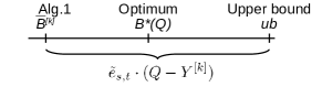
Figure 7: Illustration of the upper bound from Theorem 4.2.

∎

Proof of Proposition 4.5..

To compute the ordered LP-extremes $\mathcal{R}_{i}$ of the individual $i$ we resort to the method of Kirkpatrick and Seidel (1986) of complexity $O(\sum_{i=1}^{m}|\mathcal{N}_{i}|\cdot\log|\mathcal{R}_{i}|)$. To obtain the set $\mathcal{R}$, we just need to merge these ordered sets into an aggregated ordered set. This operation has complexity $O(|\mathcal{R}|\cdot\log m)$. The rest of the operations consists in adding to the solution the alternatives in $\mathcal{R}$, one by one, which has complexity $O(|\mathcal{R}|)$. ∎

Proof of Proposition 4.7..

By construction, Algorithm. 1 gets at each iteration the alternative with the highest incremental efficiency (Line 1). This proves the first part of the claim.

The second part of the claim can be shown geometrically. In the figure above, we represent the total incentive and social welfare calculated by the algorithm at each iteration.

Observe that the incremental efficiency $\tilde{e}^{[k]}$ is the inclination of the segment connecting $(Y^{[k-1]},B^{[k-1]})$ to $(Y^{[k]},B^{[k]})$ and that the efficiency $e^{[k]}$ is the inclination of the segment connecting $(0,0)$ to $(Y^{[k]},B^{[k]})$. It becomes then evident that the monotonicity of $\tilde{e}^{[k]}$ implies also the monotonicity of $e^{[k]}$. ∎

Proof of Corollary 4.8..

Observe that at every iteration $k$ we increase the social welfare by $\tilde{e}^{[k]}\cdot(Y^{[k+1]}-Y^{[k]})$. Therefore $B(Q)=B(Y^{[k]})+\tilde{e}^{[k]}\cdot(Y^{[k+1]}-Y^{[k]})+\tilde{e}^{[k+1]}\cdot(Y^{[k+2]}-Y^{[k+1]})+\dots$. Observing that $\tilde{e}^{[k]}$ is non increasing, we get: $B(Q)\leq B(Y^{[k]})+\tilde{e}^{[k]}\cdot\left[(Y^{[k+1]}-Y^{[k]})+(Y^{[k+2]}-Y^{[k+1]})+\dots\right]=B(Y^{[k]})+\tilde{e}^{[k]}\cdot(Q-Y^{[k]})$ ∎

Proofs of Section 5

Proof of the Proposition 5.2..

From equations (1), (3), (18) and (19), observe that

$$\delta(\mathbf{z})=\sum_{i=1}^{m}\left(V_{i,j^{*}_{i}(0)}-V_{i,j^{*}_{i}(\mathbf{z})}\right)\geq 0,$$

∎

Proof of Proposition 5.4.

Thanks to Proposition 5.2, $\delta(\mathbf{z}^{\prime})=\delta(\mathbf{z})\leq Q$. Moreover, the social welfare is also the same, i.e., $B(\mathbf{z})=B(\mathbf{z}^{\prime})$, since it only depends on the alternative chosen. This shows the proposition. ∎

Proof of Proposition 5.5.

Assume, by contradiction, that the optimal personalized-incentive policy $\mathbf{y}$ is not an optimal general policy. This would imply the existence of a policy $\mathbf{z}$ such that $B(\mathbf{z})>B(\mathbf{y})$ and $\delta(\mathbf{z})\leq Q$.

Consider now a personalized-incentive policy $\mathbf{y}^{\prime}$ such that

$$\left\{\begin{array}[]{ll}y_{i,j}^{\prime}=V_{i,j^{*}_{i}(0)}-V_{i,j},&\text{if}\>j=j^{*}_{i}(\mathbf{z})\\ y_{i,j}^{\prime}=0,&\text{otherwise}\\ \end{array}\right..$$

Then, by construction, $\mathbf{y}^{\prime}$ is such that $j^{*}_{i}(\mathbf{y}^{\prime})=j^{*}_{i}(\mathbf{z})$, $\forall i\in\mathcal{I}$.

Moreover, observe that $\mathbf{y}^{\prime}$ is such that $B(\mathbf{y}^{\prime})>B(\mathbf{y})$ and $Y(\mathbf{y}^{\prime})=\delta(\mathbf{y}^{\prime})\leq Q$. Therefore, $\mathbf{y}^{\prime}$ would be a better personalized-incentive policy than $\mathbf{y}$, which is absurd, since by construction $\mathbf{y}$ is an optimal personalized-incentive policy. ∎

Proof of Corollary 5.6.

Let $B(Q)$ be the social welfare returned by Algorithm 1 for a budget $Q$. We know from Theorem 4.2 that it is boundedly close to the social welfare $B^{*}(Q)$ obtained with an optimal personalized-incentive policy, with the following bound

$$B^{*}(Q)-B(Q)\leq\tilde{e}_{s,t}\cdot(Q-\widetilde{Q}).$$

Thanks to Proposition 5.5, $B^{*}(Q)$ is also the social welfare obtained via an optimal general policy with disutility threshold $Q$. This proves the Corollary. ∎

Proof of Proposition 5.7..

By construction, the enforcement policy $\mathbf{z}$ induce the same individual alternatives as the personalized-incentive policy $\mathbf{y}$. Then, thanks to Proposition 5.2, they have the same disutility $\delta(\mathbf{z})=\delta(\mathbf{y})\leq Q$ and achieve the same social welfare $B(\mathbf{z})=B(\mathbf{y})$. Thanks to Corollary 5.6, $B(\mathbf{y})$ is boundedly close to the optimum $B(Q)$, and so is $B(\mathbf{z})$. ∎

Proof of Theorem 5.8..

Let $\mathbf{z}$ be a policy such that $z_{i,j}=\tau(b_{i,j}-A_{i})$, with $\tau$ given by equation (22) and $A_{i}\in\mathbb{R}$.

Let $\mathbf{y}$ be the personalized-incentive policy obtained running the algorithm as explained in the statement of this theorem. Thanks to Corollary 5.6, we know that $B(\mathbf{y})$ is such that

$$B^{*}(Q)-B(\mathbf{y})\leq\tilde{e}_{s,t}\cdot(Q-\widetilde{Q}).$$ (30)

If we prove that $j^{*}_{i}(\mathbf{y})=j^{*}_{i}(\mathbf{z})$, $\forall i\in\mathcal{I}$, we could claim that $B(\mathbf{z})=B(\mathbf{y})$ and also, thanks to Proposition 5.2, that $\delta(\mathbf{z})=\delta(\mathbf{y})\leq Q$. In this case, the bound (30) would also hold for $\mathbf{z}$.

To do so, we show that (i) alternative $j^{*}_{i}(\mathbf{z})$ is in the set $\mathcal{R}_{i}$ of the LP-extremes alternatives and (ii) alternative $j^{*}_{i}(\mathbf{y})$ maximizes $U_{i,j}(\mathbf{z})=V_{i,j}+\tau(b_{i,j}-A_{i})$, over all alternatives $j\in\mathcal{R}_{i}$.

Proof of (i)

Assume, by contradiction, that $j^{*}_{i}(\mathbf{z})$ is LP dominated by alternatives $j$ and $j^{\prime}$, i.e., $b_{i,j}<b_{i,j^{*}_{i}(\mathbf{z})}<b_{i,j^{\prime}}$ and $y_{i,j}<y_{i,j^{*}_{i}(\mathbf{z})}<y_{i,j^{\prime}}$, and

$$\frac{b_{i,j^{\prime}}-b_{i,j^{*}_{i}(\mathbf{z})}}{w_{i,j^{\prime}}-w_{i,j^{*}_{i}(\mathbf{z})}}\geq\frac{b_{i,j^{*}_{i}(\mathbf{z})}-b_{i,j}}{w_{i,j^{*}_{i}(\mathbf{z})}-w_{i,j}}.$$

From equation (8), $w_{i,j}=V_{i,j^{*}_{i}(0)}-V_{i,j}$ and thus the previous condition can be written as

$$\frac{b_{i,j^{\prime}}-b_{i,j^{*}_{i}(\mathbf{z})}}{V_{i,j^{*}_{i}(\mathbf{z})}-V_{i,j^{\prime}}}\geq\frac{b_{i,j^{*}_{i}(\mathbf{z})}-b_{i,j}}{V_{i,j}-V_{i,j^{*}_{i}(\mathbf{z})}}.$$

Multiplying by $\tau>0$ on both sides and adding and subtracting $A_{i}$ yields

$$\tau\frac{b_{i,j^{\prime}}-b_{i,j^{*}_{i}(\mathbf{z})}-A+A}{V_{i,j^{*}_{i}(\mathbf{z})}-V_{i,j^{\prime}}}\geq\tau\frac{b_{i,j^{*}_{i}(\mathbf{z})}-b_{i,j}-A+A}{V_{i,j}-V_{i,j^{*}_{i}(\mathbf{z})}}.$$

Rearranging the terms and using equation (21) yields

$$\frac{z_{i,j^{\prime}}-z_{i,j^{*}_{i}(\mathbf{z})}}{V_{i,j^{*}_{i}(\mathbf{z})}-V_{i,j^{\prime}}}\geq\frac{z_{i,j^{*}_{i}(\mathbf{z})}-z_{i,j}}{V_{i,j}-V_{i,j^{*}_{i}(\mathbf{z})}}.$$

Finally, using equation (1), we get

$$\frac{U_{i,j^{\prime}}(\mathbf{z})-U_{i,j^{*}_{i}(\mathbf{z})}(\mathbf{z})}{V_{i,j^{*}_{i}(\mathbf{z})}-V_{i,j^{\prime}}}\geq\frac{U_{i,j^{*}_{i}(\mathbf{z})}(\mathbf{z})-U_{i,j}(\mathbf{z})}{V_{i,j}-V_{i,j^{*}_{i}(\mathbf{z})}}.$$

Let $\alpha=V_{i,j}-V_{i,j^{*}_{i}(\mathbf{z})}$ and $\alpha^{\prime}=V_{i,j^{*}_{i}(\mathbf{z})}-V_{i,j^{\prime}}$. From $y_{i,j}<y_{i,j^{*}_{i}(\mathbf{z})}<y_{i,j^{\prime}}$, it follows that $V_{i,j}>V_{i,j^{*}_{i}(\mathbf{z})}>V_{i,j^{\prime}}$ and thus $\alpha,\alpha^{\prime}>0$. Then, we get

$$\frac{U_{i,j^{\prime}}(\mathbf{z})-U_{i,j^{*}_{i}(\mathbf{z})}(\mathbf{z})}{\alpha^{\prime}}\geq\frac{U_{i,j^{*}_{i}(\mathbf{z})}(\mathbf{z})-U_{i,j}(\mathbf{z})}{\alpha}.$$

By simple arithmetic calculation, one can see that this is equivalent to

$$\frac{\alpha U_{i,j^{\prime}}(\mathbf{z})+\alpha^{\prime}U_{i,j}(\mathbf{z})}{\alpha+\alpha^{\prime}}\geq U_{i,j^{*}_{i}(\mathbf{z})}(\mathbf{z}).$$ (31)

Equation (31) means that the utility of $j^{*}_{i}(\mathbf{z})$ is less than or equal to the weighted average of the utility of $j$ and $j^{\prime}$. Two cases could then hold:

• Either $j$ or $j^{\prime}$ is preferred to $j^{*}_{i}(\mathbf{z})$, i.e., $U_{i,j}(\mathbf{z})>U_{i,j^{*}_{i}(\mathbf{z})}(\mathbf{z})$ or $U_{i,j^{\prime}}(\mathbf{z})>U_{i,j^{*}_{i}(\mathbf{z})}(\mathbf{z})$. This would mean that $j^{*}_{i}(\mathbf{z})$ does not maximizes utility and would contradict equation (4).

• The three alternatives are equivalent, i.e., $U_{i,j}(\mathbf{z})=U_{i,j^{*}_{i}(\mathbf{z})}(\mathbf{z})=U_{i,j^{\prime}}(\mathbf{z})$. This would also contradict equation (4) because $b_{i,j^{\prime}}>b_{i,j^{*}_{i}(\mathbf{z})}$, by assumption.

Therefore, $j^{*}_{i}(\mathbf{z})$ is not a LP-dominated alternative. Clearly, $j^{*}_{i}(\mathbf{z})$ is not dominated either and thus $j^{*}_{i}(\mathbf{z})\in\mathcal{R}_{i}$.

Proof of (ii)

The proof of (ii) requires the following lemmas.

Lemma A If the alternatives in $\mathcal{R}_{i}$ are ordered according to equation (11), i.e., they are ordered by increasing weight, then

$$\tilde{e}_{i,1}>\tilde{e}_{i,2}>\dots>\tilde{e}_{i,r_{i}}.$$

To prove this lemma, show by contradiction that if $\tilde{e}_{i,j}\leq\tilde{e}_{i,j+1}$, then $j$ would be LP-dominated by $j-1$ and $j+1$.

Lemma B If $j\in\mathcal{R}_{i}$ is such that $\tilde{e}_{i,j}\geq 1/\tau$, then $U_{i,j-1}(\mathbf{z})\leq U_{i,j}(\mathbf{z})$, where $j-1$ denotes the alternative which comes just before $j$ in the ordered set $\mathcal{R}_{i}$.

To prove this lemma, note that, using equations (8), (12) and (13), the inequality $\tilde{e}_{i,j}\geq 1/\tau$ can be written as

$$\frac{b_{i,j}-b_{i,j-1}}{V_{i,j-1}-V_{i,j}}\geq 1/\tau.$$

Multiplying by $\tau(V_{i,j}-V_{i,j-1})>0$, subtracting $\tau\cdot A_{i}$ from both sides and rearranging the terms, we get $V_{i,j-1}-\tau(A-b_{i,j-1})\leq V_{i,j}-\tau(A-b_{i,j})$. Using equations (21) and (1) yields $U_{i,j-1}(\mathbf{z})\leq U_{i,j}(\mathbf{z})$.

Lemma C If $j\in\mathcal{R}_{i}$ is such that $\tilde{e}_{i,j}<1/\tau$, then $U_{i,j-1}(\mathbf{z})>U_{i,j}(\mathbf{z})$, where $j-1$ denotes the alternative which comes just before $j$ in the ordered set $\mathcal{R}_{i}$.

This lemma can be proved with the same reasoning as Lemma B.

Let $j\in\mathcal{R}_{i}$ be such that

$$\tilde{e}_{i,j}\geq 1/\tau>\tilde{e}_{i,j+1}.$$ (32)

Then, Lemmas A and B imply that the alternatives in the set $\{{j^{\prime}}\in\mathcal{R}_{i}:\>{j^{\prime}}\leq j\}$ are ordered by non-decreasing utility. Similarly, Lemmas A and C imply that the alternatives in the set $\{{j^{\prime}}\in\mathcal{R}_{i}:\>{j^{\prime}}\geq j\}$ are ordered by decreasing utility. Hence, alternative $j$, defined by equation (32), is the alternative which maximizes the utility $U_{i,j}(\mathbf{z})$, over all alternatives in $\mathcal{R}_{i}$.

Observe that, by construction of Algorithm 1, the alternative $j^{*}_{i}(\mathbf{y})$ satisfies equation (32). Hence, alternative $j^{*}_{i}(\mathbf{y})$ maximizes the utility $U_{i,j}(\mathbf{z})$, over all alternatives $j\in\mathcal{R}_{i}$. As we have shown that $j^{*}_{i}(\mathbf{z})\in\mathcal{R}_{i}$, it must be that $j^{*}_{i}(\mathbf{y})=j^{*}_{i}(\mathbf{z})$. ∎

Proof of Proposition 5.9..

For any individual $i\in\mathcal{I}$, let us consider the alternative $j^{*}_{i}(\mathbf{z})$ she chooses under policy $\mathbf{z}$ and compute the respective incentive

$$z_{i,j^{*}_{i}(\mathbf{z})}=\tau\cdot(b_{i,j^{*}_{i}(\mathbf{z})}-A_{i})\geq\tau\cdot(b_{i,j^{*}_{i}(\mathbf{z})}-b_{i,j^{*}_{i}(0)})\geq V_{i,j^{*}_{i}(0)}-V_{i,j^{*}_{i}(\mathbf{z})}.$$

where the first inequality is a consequence of the definition of proportional-incentive policy – see (23), while the last inequality ensures that the incentive compensates for the loss in individual utility when shifting to alternative $j^{*}_{i}(\mathbf{z})$, which is a necessary condition for the individual to accept the incentive and shift to $j^{*}_{i}(\mathbf{z})$.

Therefore, recalling from Definition 4.1 that the efficiency of a generic alternative $j$ as $e_{i,j}\equiv\frac{b_{i,j}-b_{i,j^{*}_{i}(0)}}{V_{i,j^{*}_{i}(0)}-V_{i,j}}$, we can write:

$$\frac{1}{\tau}\leq e_{i,j^{*}_{i}(\mathbf{z})},\ \ \forall i\in\mathcal{I}\quad\Longrightarrow\quad\frac{1}{\tau}\leq\min_{i\in\mathcal{I}}e_{i,j^{*}_{i}(\mathbf{z})}$$

Observe that the smaller $\tau$, the smaller the incentive spent by $\mathbf{z}$. Therefore, it is always best to choose

$$\tau=\frac{1}{\min_{i\in\mathcal{I}}e_{i,j^{*}_{i}(\mathbf{z})}}$$

Let us now consider a policy $\mathbf{y}$ that incentivizes the same individuals $i\in\mathcal{I}$. In particular, it incentivizes the same alternative $j^{*}_{i}(\mathbf{z})$, with a quantity $y_{i,j^{*}_{i}(\mathbf{z})}=V_{i,j^{*}_{i}(0)}-V_{i,j^{*}_{i}(\mathbf{z})}$. This incentive is sufficient to induce each individual to choose such an alternative. Therefore, the social welfare of this new policy $\mathbf{y}$ will be the same as $\mathbf{z}$, i.e., $B(\mathbf{y})=B(\mathbf{z})$. However, the saving of incentive distributed is:

$$Y(\mathbf{z})-Y(\mathbf{y}) =\sum_{i\in\mathcal{I}}(z_{i,j^{*}_{i}(\mathbf{z})}-y_{i,j^{*}_{i}(\mathbf{z})})=\sum_{i\in\mathcal{I}}(b_{i,j^{*}_{i}(\mathbf{z})}-b_{i,j^{*}_{i}(0)})\cdot\left(\tau-\frac{1}{e_{i,j^{*}_{i}(\mathbf{z})}}\right)$$

$$=\frac{1}{\tau}\cdot\sum_{i\in\mathcal{I}}\frac{b_{i,j^{*}_{i}(\mathbf{z})}-b_{i,j^{*}_{i}(0)}}{e_{i,j^{*}_{i}(\mathbf{z})}}\cdot\left(e_{i,j^{*}_{i}(\mathbf{z})}-\frac{1}{\tau}\right)=\frac{1}{\tau}\cdot\sum_{i\in\mathcal{I}}\left(V_{i,j^{*}_{i}(\mathbf{z})}-V_{i,j^{*}_{i}(0)}\right)\cdot\Delta e_{i,j^{*}_{i}(\mathbf{z})}$$

∎

Proof of Proposition 5.10.

Let us run Algorithm 1 with budget $Q=Y(\mathbf{z})$, which allows to get the values of $\tilde{e}_{Y(\mathbf{z})}$ and $\gamma_{Y(\mathbf{z})}$. Thanks to Proposition 5.9, there always exists a personalized-incentive policy policy $\mathbf{y}$ that achieves at least the same social welfare of $\mathbf{z}$:

$$B(\mathbf{y})\geq B(\mathbf{z})$$ (33)

while providing incentive savings of at lest $L(\mathbf{z})$. Let $k^{\prime}$ be the first iteration of the algorithm in which $Y^{[k^{\prime}]}\geq Y(\mathbf{y})$ and $k^{\prime\prime}$ the last iteration in which $Y^{[k^{\prime\prime}]}\leq Y(\mathbf{z})$.

First, suppose $L(\mathbf{z})\geq 2\gamma_{Y(\mathbf{z})}$. In this case, observe that

$$Y^{[k^{\prime}]}-Y(\mathbf{y}) \leq\gamma_{Y(\mathbf{z})}$$

$$Y(\mathbf{z})-Y^{[k^{\prime\prime}]} \leq\gamma_{Y(\mathbf{z})}$$

$$Y(\mathbf{z})-Y(\mathbf{y}) \geq L(\mathbf{z}).$$

This is shown, for the sake of understanding, in the following figure

Summing the first two of the inequalities above and then replacing $Y(\mathbf{z})-Y(\mathbf{y})$ with the third inequality, we get

$$Y^{[k^{\prime}]}-Y^{[k^{\prime\prime}]}+L(\mathbf{z})\leq Y^{[k^{\prime}]}-Y(\mathbf{y})+Y(\mathbf{z})-Y^{[k^{\prime\prime}]}\leq 2\gamma_{Y(\mathbf{z})}$$

Rearranging the elements between the first and third terms, we get

$$Y^{[k^{\prime\prime}]}-Y^{[k^{\prime}]}\geq L(\mathbf{z})-2\gamma_{Y(\mathbf{z})}.$$ (34)

Observe that:

$$B^{[k^{\prime\prime}]}-B^{[k^{\prime}]} =\sum_{k=k^{\prime}}^{k^{\prime\prime}-1}(B^{[k+1]}-B^{[k]})$$

$$=\sum_{k=k^{\prime}}^{k^{\prime\prime}-1}\tilde{e}^{[k]}\cdot(Y^{[k+1]}-Y^{[k]})\geq\tilde{e}^{[k^{\prime\prime}]}$$

$$=\sum_{k=k^{\prime}}^{k^{\prime\prime}-1}(Y^{[k+1]}-Y^{[k]})$$

$$=\tilde{e}^{[k^{\prime\prime}]}\cdot(Y^{[k^{\prime\prime}]}-Y^{[k^{\prime}]})$$

where the inequality holds thanks to the monotonicity of incremental efficiencies (Proposition 4.7). Applying (34):

$$B^{[k^{\prime\prime}]}-B^{[k^{\prime}]}\geq\tilde{e}^{[k^{\prime\prime}]}\cdot(L(\mathbf{z})-2\gamma_{Y(\mathbf{z})})$$

By construction, $\tilde{e}^{[k^{\prime\prime}]}=\tilde{e}_{Y(\mathbf{z})}$. Moreover, $B^{*}(Y(\mathbf{z}))\geq B^{*}(Y^{[k^{\prime\prime}]})=B^{[k^{\prime\prime}]}$, where the inequality holds thanks to the monotonicity of the maximum social welfare curve and the equality holds thanks to Corollary 4.4 . We also know that $B^{[k^{\prime}]}=B^{*}(Y^{[k^{\prime}]})\geq B^{*}(Y(\mathbf{y}))\geq B(\mathbf{y})\geq B(\mathbf{z})$, where the first equality derives from Corollary 4.4, the second inequality from the monotonicity of the maximum social welfare curve, the third inequality by the definition of optimal personalized-incentive policy and the last by (33).

∎

Proofs of Section 6

Proof of Proposition 6.1..

Let $\xi=\epsilon_{i,j^{*}_{i}(0)}-\epsilon_{i,j}$. Then, $\xi$ is the difference of two i.i.d. Gumbel-distributed random variables with scale parameter $\mu$, and thus it is a logistic-distributed random variable with scale parameter $\mu$ (Nadarajah and Kotz 2005). Its probability density function is $f(x)=\frac{e^{x/\mu}}{\mu(e^{x/\mu}+1)^{2}}$ and its cumulative distribution function is $F(x)=\frac{e^{x/\mu}}{e^{x/\mu}+1}$. For any $z\in\mathbb{R}$, we have

$$\mathbb{E}(\xi|\xi>z)= \frac{\int_{z}^{\infty}xf(x)dx}{1-F(z)}$$

$$= \frac{1}{1-e^{z/\mu}/(1+e^{z/\mu})}\int_{z}^{\infty}\frac{xe^{x/\mu}}{\mu(e^{x/\mu}+1)^{2}}dx$$

$$= \left(1+e^{z/\mu}\right)\int_{z}^{\infty}\frac{xe^{x/\mu}}{\mu(e^{x/\mu}+1)^{2}}dx.$$

Using

$$\frac{\partial}{\partial x}\left(-\frac{x}{e^{x/\mu}+1}\right)=\frac{xe^{x/\mu}}{\mu(e^{x/\mu}+1)^{2}}-\frac{1}{e^{x/\mu}+1},$$

and

$$\frac{\partial}{\partial x}\mu\ln(1+e^{-x/\mu})=\frac{-e^{-x/\mu}}{1+e^{-x/\mu}}=\frac{-1}{e^{x/\mu}+1},$$

we get

$$\int_{z}^{\infty}\frac{xe^{x/\mu}}{\mu(e^{x/\mu}+1)^{2}}dx =\frac{z}{e^{z/\mu}+1}-\int_{z}^{\infty}\frac{-1}{e^{x/\mu}+1}dx.$$

$$=\frac{z}{e^{z/\mu}+1}+\mu\ln(1+e^{-z/\mu}).$$

Finally,

$$y_{i,j} =\hat{y}_{i,j}+\mathbb{E}(\xi|\xi>-\hat{y}_{i,j})$$

$$=\hat{y}_{i,j}-\hat{y}_{i,j}+\mu(1+e^{-\hat{y}_{i,j}/\mu})\ln(1+e^{\hat{y}_{i,j}/\mu})$$

$$=\mu\frac{1+e^{\hat{y}_{i,j}/\mu}}{e^{\hat{y}_{i,j}/\mu}}\ln(1+e^{\hat{y}_{i,j}/\mu}).$$

∎

Appendix C Census Data Description

We now describe the census data we use. They are published by INSEE and concern the period from 2015 to 2019. The data contain observations for $7\,861\,201$ households, representing $21\,810\,707$ individuals (about a third of national population). Only one individual is surveyed in each household, which means that, for example, the main mode of transportation is only observed for one individual in the household. Hence, in each household, we consider only the surveyed individual.

We restrict our sample to workers living and working in the Rhône department, with a valid mode of transportation (i.e., unemployed and individuals working from home are excluded). We remove some outliers, i.e., individuals travelling more than 90 minutes, which were about $2000$. The final dataset contains $221\,571$ individuals. The total number of alternatives is $1\,092\,748$.

Note that census data do not represent an exhaustive sample of the population. Therefore, some categories of individuals might be over- or under-represented. To correct for such imbalances, INSEE computes a weight for each surveyed person. To compute the statistics below and to perform the multinomial regression, we use these weights.

Home and Work Location.

The home and work location of the individuals is reported at the city-level, except for Lyon where it is reported at the district-level. There are $275$ unique home locations (an average of $812$ individuals living at each location).

Mode of Transportation.

The main mode of transportation used for commuting is in one of the following five categories: car, public transit, walking, cycling and motorcycle. The share of each category are reported on Table 6.

Table 6: Share of each mode of transportation reported.

Mode of transportation	Share
Car	$60.69\text{\,}\%$
Public transit	$25.07\text{\,}\%$
Walking	$8.83\text{\,}\%$
Cycling	$3.95\text{\,}\%$
Motorcycle	$1.47\text{\,}\%$

Source: population census for Rhône department, INSEE.

Socio-Demographic Variables.

The data contain socio-demographic variables which are used to estimate a Multinomial Logit model for mode choice. Table 7 reports the list of numeric variables that we use, Table 8 reports the list of categorical variables that we use.

Table 7: Description of the numeric socio-demographic variables.

Name	Description	Mean
Age	Age of the individual, rounded to the nearest five-year age group	$38.49$
Cars per individual	Number of cars owned divided by number of employed in the household	$0.84$

Source: population census for Rhône department, INSEE.

Table 8: Description of the categorical socio-demographic variables.

Name	Description	Most frequent category
Sex	Sex of the individual	man ($50.67\text{\,}\%$)
Occupation	Occupation of the individual, using INSEE nomenclature	employee ($24.93\text{\,}\%$)

Source: population census for Rhône department, INSEE.

Appendix D Computation of Travel Times

For any individual, the origin point of her trips is set to the town hall of the city where she lives and the destination point is set to the town hall of the city where she works (for district-level home and workplace, the town hall of the district is used). The coordinates of the town halls are retrieved from OpenStreetMap.

Travel time of each mode is set to the travel time of the fastest path, within that mode, which connects the two locations, computed from the open-source routing engine GraphHopper. The road network for pedestrians, bicycles, motorcycles and cars is retrieved from OpenStreetMap data. It is assumed that there is no congestion. For public transit trips, the fastest path is computed using public transit timetables, retrieved from open-data GTFS files. The departure time is assumed to be at 8 a.m. on a weekday.

Note that, for some individuals, no path can be found to travel by public transit from their origin to their destination ($16\,161$ individuals, representing 10.87% of total sample weight). For these individuals, we exclude public transit from their choice set.

Some individuals are living and working in the same city ($61\,497$ individuals, representing $26.61\text{\,}\%$ of total sample weight). For these individuals, travel times are computed by supposing that trip distance is equal to the radius of the city (assuming cities are circular) and that speed is equal to the average speed of intercity trips.

Figure 8 shows the distribution of travel times in the population, for each mode of transportation. Except for public transit trips, most trips last less than 30 minutes.

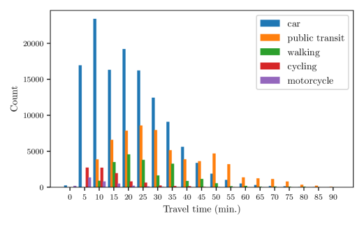
Figure 8: Distribution of travel times in the population (before the policy).

Appendix E Simulating Utilities

In the Multinomial Logit model, the utility of individual $i$ with mode of transportation $j$ is

$$V_{i,j}=\hat{V}_{i,j}+\epsilon_{i,j},$$

where $\hat{V}_{i,j}$ is the deterministic part of the utility, which depends on the individual- and alternative-specific exogenous variables, and $\epsilon_{i,j}$ is a random variable with standard Gumbel distribution.

The deterministic part $\hat{V}_{i,j}$ are computed from the estimates of the Multinomial Logit model. From the data, we know the alternative $j^{*}_{i}(0)$ chosen by any individual $i$ so we must have

$$V_{i,j^{*}_{i}(0)}>V_{i,j},\quad\forall j\neq j^{*}_{i}(0).$$ (35)

To simulate draws of standard Gumbel variables conditional on equation (35), we use the rejection sampling method, i.e., we draw values from the standard Gumbel distribution until the constraint of equation (35) is satisfied.

References

- Anderson, de Palma, and Thisse (1992) Anderson, Simon P, André de Palma, and Jacques François Thisse. 1992. Discrete choice theory of product differentiation. MIT press.
- Araldo, Di Stefano, and Di Stefano (2020) Araldo, A., A. Di Stefano, and A. Di Stefano. 2020. “Resource Allocation for Edge Computing with Multiple Tenant Configurations.” In ACM/SIGAPP Symposium On Applied Computing, .
- Araldo et al. (2019) Araldo, A., S.l Gao, R. Seshadri, C. Lima Azevedo, H. Ghafourian, Y. Sui, S. Ayaz, D. Sukhin, and M. Ben-Akiva. 2019. “System-level optimization of multi-modal transportation networks for energy efficiency using personalized incentives.” Transportation Research Records 2673 (12).
- Arcep (2021) Arcep. 2021. “Le plan France Très Haut Débit.” https://www.arcep.fr/demarches-et-services/collectivites/le-plan-france-tres-haut-debit-pfthd.html.
- Cao, Brahma, and Varshney (2015) Cao, Nianxia, Swastik Brahma, and Pramod K. Varshney. 2015. “Target tracking via crowdsourcing: A mechanism design approach.” IEEE Transactions on Signal Processing 63 (6): 1464–1476.
- Chester, Horvath, and Madanat (2010) Chester, Mikhail V., Arpad Horvath, and Samer Madanat. 2010. “Comparison of life-cycle energy and emissions footprints of passenger transportation in metropolitan regions.” Atmospheric Environment 44 (8): 1071–1079. http://dx.doi.org/10.1016/j.atmosenv.2009.12.012.
- Clarke and Margetts (2014) Clarke, Amanda, and Helen Margetts. 2014. “Governments and citizens getting to know each other? Open, closed, and big data in public management reform.” Policy & Internet 6 (4): 393–417.
- Colorni et al. (2017) Colorni, Alberto, Valentina Ferretti, Alessandro Luè, Alessandra Oppio, Valerio Paruscio, and Luca Tomasini. 2017. “Rethinking feasibility analysis for urban development: A multidimensional decision support tool.” In Computational Science and its Applications - ICCSA, .
- De Borger (2001) De Borger, Bruno. 2001. “Discrete choice models and optimal two-part tariffs in the presence of externalities: optimal taxation of cars.” Regional Science and Urban Economics 31 (4): 471–504.
- Ettema, Knockaert, and Verhoef (2010) Ettema, Dick, Jasper Knockaert, and Erik Verhoef. 2010. “Using incentives as traffic management tool: empirical results of the peak avoidance experiment.” Transportation Letters 2 (1): 39–51.
- Fielder et al. (2016) Fielder, Andrew, Emmanouil Panaousis, Pasquale Malacaria, Chris Hankin, and Fabrizio Smeraldi. 2016. “Decision support approaches for cyber security investment.” Decision Support Systems 86: 13–23. http://dx.doi.org/10.1016/j.dss.2016.02.012.
- Hu, Chiu, and Zhu (2015) Hu, Xianbiao, Yi Chang Chiu, and Lei Zhu. 2015. “Behavior Insights for an Incentive-Based Active Demand Management Platform.” International Journal of Transportation Science and Technology 4 (2): 119–133. http://dx.doi.org/10.1260/2046-0430.4.2.119.
- Inoa, Picard, and de Palma (2015) Inoa, Ignacio A, Nathalie Picard, and André de Palma. 2015. “Effect of an accessibility measure in a model for choice of residential location, workplace, and type of employment.” Mathematical Population Studies 22 (1): 4–36.
- Javaudin, Araldo, and de Palma (2022) Javaudin, Lucas, Andrea Araldo, and André de Palma. 2022. “Large-scale allocation of personalized incentives.” In 2022 IEEE 25th International Conference on Intelligent Transportation Systems (ITSC), 4151–4156. IEEE.
- Kellerer et al. (2004) Kellerer, Hans, et al. 2004. Knapsack Problems. 1st ed. Springer.
- Kirkpatrick and Seidel (1986) Kirkpatrick, David G, and Raimund Seidel. 1986. “The Ultimate Planar Convex Hull Algorithm?” SIAM J. Comput. 15 (1): 1–18. http://ecommons.cornell.edu/handle/1813/6417.
- Levy and Le Jeannic (2011) Levy, David, and Thomas Le Jeannic. 2011. “Un habitant de pôle urbain émet deux fois moins de CO2 que la moyenne pour se rendre à son lieu de travail ou d’études.” INSEE Première .
- Merugu, Prabhakar, and Rama (2009) Merugu, Deepak, Balaji S Prabhakar, and N Rama. 2009. “An incentive mechanism for decongesting the roads: A pilot program in bangalore.” In Proc. of ACM NetEcon Workshop, Citeseer.
- Mirhedayatian and Yan (2018) Mirhedayatian, Seyed Mostafa, and Shiyu Yan. 2018. “A framework to evaluate policy options for supporting electric vehicles in urban freight transport.” Transportation Research Part D: Transport and Environment 58 (November 2017): 22–38. https://doi.org/10.1016/j.trd.2017.11.007.
- Mohammadivojdan and Geunes (2018) Mohammadivojdan, Roshanak, and Joseph Geunes. 2018. “The newsvendor problem with capacitated suppliers and quantity discounts.” European Journal of Operational Research 271 (1): 109–119. https://doi.org/10.1016/j.ejor.2018.05.015.
- Muñoz, Monzon, and Daziano (2016) Muñoz, Begoña, Andres Monzon, and Ricardo A Daziano. 2016. “The increasing role of latent variables in modelling bicycle mode choice.” Transport Reviews 36 (6): 737–771.
- Nadarajah and Kotz (2005) Nadarajah, Saralees, and Samuel Kotz. 2005. “A generalized logistic distribution.” International Journal of Mathematics and Mathematical Sciences 2005 (19): 3169–3174.
- Quinet et al. (2009) Quinet, Alain, Luc Baumstark, Joffrey Célestin-Urbain, Hervé Pouliquen, Dominique Auverlot, and Christine Raynard. 2009. “La valeur tutélaire du carbone.” Rapport du Conseil d’Analyse Stratégique 16 (5): 9305.
- Small and Rosen (1981) Small, Kenneth A., and Harvey S. Rosen. 1981. “Applied Welfare Economics with Discrete Choice Models.” Econometrica 49 (1): 105–130.
- Sun et al. (2020) Sun, Jian, Jiyan Wu, Feng Xiao, Ye Tian, and Xiangdong Xu. 2020. “Managing bottleneck congestion with incentives.” Transportation Research Part B: Methodological 134: 143–166. https://doi.org/10.1016/j.trb.2020.01.010.
- Tang et al. (2020) Tang, Yili, Yu Jiang, Hai Yang, and Otto Anker Nielsen. 2020. “Modeling and optimizing a fare incentive strategy to manage queuing and crowding in mass transit systems.” Transportation Research Part B: Methodological 138: 247–267.
- Wardman et al. (2012) Wardman, Mark, Phani Chintakayala, Gerard de Jong, and Diego Ferrer. 2012. “European wide meta-analysis of values of travel time.” ITS, University of Leeds, Paper prepared for EIB .
- Yue et al. (2015) Yue, Jia Shuo, Chinmoy V Mandayam, Deepak Merugu, Hossein Karkeh Abadi, and Balaji Prabhakar. 2015. “Reducing road congestion through incentives: a case study.” In Transportation Research Board 94th Annual Meeting, Washington, DC, .
- Zhang (2020) Zhang, Junyi. 2020. “Transport policymaking that accounts for COVID-19 and future public health threats: A PASS approach.” Transport policy 99: 405–418.
- Zhong and Young (2010) Zhong, Tao, and Rhonda Young. 2010. “Multiple Choice Knapsack Problem: Example of planning choice in transportation.” Evaluation and Program Planning 33 (2): 128–137.
- Zoltners, Sinha, and Chong (1979) Zoltners, Andris A., Prabhakant Sinha, and Philip S. C. Chong. 1979. “An Optimal Algorithm for Sales Representative Time Management.” Management Science 25 (12): 1197–1207.