Analytic solution for pulse wave propagation in flexible tubes with application to patient-specific arterial tree

Abstract

In this paper, we present an analytic solution for pulse wave propagation in a flexible arterial model with tapering, physiological boundary conditions and variable wall properties (wall elasticity and thickness). The change of wall properties follows a profile that is proportional to $r^{\alpha}$, where $r$ represents the lumen radius and $\alpha$ is a material coefficient. The cross-sectionally averaged velocity and pressure are obtained by solving a hyperbolic system derived from the mass and momentum conservations, and they are expressed in Bessel functions of order $(4-\alpha)/(3-\alpha)$ and $1/(3-\alpha)$, respectively. The solution is successfully validated by comparing it with numerical results from 3D fluid-structure interaction simulations. Subsequently, the solution is employed to study pulse wave propagation in an arterial model, revealing that the wall properties and the physiological outlet boundary conditions, such as the RCR model, play a crucial role in characterizing the input impedance and reflection coefficient. At low-frequency range, the input impedance is found to be insensitive to the wall properties and is primarily determined by the RCR parameters. At high-frequency range, the input impedance oscillates around the local characteristic impedance, and the oscillation amplitude varies non-monotonically with $\alpha$. Expressions for the input impedance at both low-frequency and high-frequency limits are presented. This analytic solution is also successfully applied to model flow inside a patient-specific arterial tree, with the maximum relative errors in pressure and flow rate never exceeding $1.6\%$ and $9.0\%$ when compared to results from 3D numerical simulation.

Keywords Blood flow  $\cdot$ Biological fluid dynamics  $\cdot$ Flow-vessel interactions

1 Introduction

The pumping action of the heart creates pulse waves within the arterial system. The characteristics of pulse wave propagation is critical in understanding the behavior and functionality of arteries and, therefore, cardiovascular fitness (Safar et al., 2003; van de Vosse and Stergiopulos, 2011). Pulse wave propagation has been studied extensively through experiments (Moens, 1878; Segers and Verdonck, 2000; Bessems et al., 2008), theoretical analysis (Korteweg, 1878; Womersley, 1955, 1957; Papadakis, 2011) and numerical simulations (Alastruey et al., 2011; Mynard and Smolich, 2015; Charlton et al., 2019; Zimmermann et al., 2021).

In theoretical studies, the artery is commonly modeled as a straight flexible tube with uniform thickness and elasticity (Womersley, 1955, 1957; Atabek and Lew, 1966; Lighthill, 2001; Flores et al., 2016). However, the radius and thickness of the artery usually decrease along the blood flow direction, while the wall elasticity increases. It is known that these factors can change the local impedance of the artery and affect pulse wave propagation (Myers and Capper, 2004; Vlachopoulos et al., 2011). Also, arteries typically terminate at a bifurcation or connect to a vascular bed, resulting in an intricate outlet impedance that is commonly neglected in theoretical analysis.

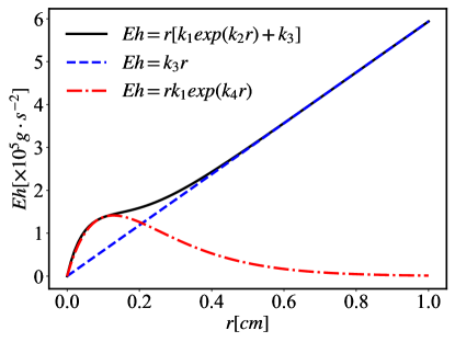
Figure 1: Relationship between $Eh$ and lumen radius of a healthy 30-year-old human subject with $k_{1}=$ $3\times 10^{6}g\cdot cm^{-1}\cdot s^{-2}$, $k_{2}=-13.5cm^{-1}$, $k_{3}=5.94\times 10^{5}g\cdot cm^{-1}\cdot s^{-2}$ and $k_{4}=-7.8cm^{-1}$ (Charlton et al., 2019).

For human arteries, tapering is usually mild, with the tapering angle not exceeding $1.5^{\circ}$ (Segers and Verdonck, 2000; Papadakis, 2011). In terms of wall properties, as will be shown in section 2, it is actually the product of the elastic modulus $E$ and the wall thickness $h$ that determines the overall property of the vessel wall. Hence, $Eh$ is sometimes called the arterial stiffness (Charlton et al., 2019). Experimental research shows that $Eh$ can be approximated by the following function of the local lumen radius $r$

$$Eh=r\left[k_{1}\exp(k_{2}r)+k_{3}\right],$$ (1)

where $k_{1}$, $k_{2}$ and $k_{3}$ are fitting parameters (Olufsen, 1999). This wall property profile is widely adopted in 1D numerical studies (Mynard and Smolich, 2015; Charlton et al., 2019). Figure 1 shows $Eh$ for a young healthy subject using this function. It can be seen that $Eh$ can be approximated by a linear function when the vessel radius is greater than $2mm$, which is true for most major arteries. It can be approximated by an exponential function instead when the vessel radius is less than $2mm$. Moreover, other researchers (Reymond et al., 2009; Willemet et al., 2015) have assumed that the relationship between $Eh$ and the local radius can be characterized by the following power-law function

$$Eh=k_{1}\overline{r}^{k_{2}}$$ (2)

where $\overline{r}$ represents the time-averaged radius of the artery.

Among the aforementioned factors, tapering of the blood vessel probably receives the most attention. The first theoretical treatment of tapering is presented by Evans (1960). The author found that it would cause constant reflection of the forward wave and claimed that only by considering tapering that we could explain the discrepancy between the pulse wave velocity predicted from existing theory and experimental measurements. However, in order to get an analytic solution, the vessel distensibility was assumed to be constant along the tapered vessel in this study, which is considered invalid from a modern perspective. Patel et al. (1963) investigated the effect of tapering on pulse wave propagation in an animal experiment. By measuring the pressure-radius ($P-R$) relationship along the aorta of 30 dogs, they found that $\Delta P/\Delta R$, a measurement of local impedance, decreased as the mean radius reduced downstream of the aorta. Lighthill (1975) modeled the tapering of a vessel using a series of compact sections of straight tubes with stepwise diameter reduction and directly applied the solution from straight tubes to each section to study the pulse wave propagation. Abdullateef et al. (2021) investigated the effect of tapering using 1D numerical simulations in time domain and confirmed that tapering would induce constant reflections which would led to increased pulse pressure amplification. They also studied the effect of modeling tapering with stepwise diameter reduction and concluded that this approach would cause artificial oscillations compared with smooth tapering. The wall properties (elasticity and thickness) were assumed to be uniform in their study. Papadakis (2011) started from the Navier-Stokes equation in the spherical coordinate system and derived the closed-form analytic solution for a tapered vessel with uniform wall properties. The pressure and velocity were expressed with the Bessel functions of orders 4/3 and 1/3. Segers and Verdonck (2000) conducted experiments with hydraulic models made up of tapering tubes with uniform wall properties and also carried out theoretical analysis using the transmission line theory. They concluded that the aortic wave reflection indices from in vivo measurements were resulted from the continuous wave reflection from tapering and local reflections from the branches.

As for wall properties, Myers and Capper (2004) accounted for both the geometric and elastic tapering in arteries by assuming the characteristic impedance and the propagation constant varied exponentially with the axial distance. The nonlinear Riccati equation for the input impedance was derived and solved to obtain the flow and pressure inside the model with the help of the transmission line method. Wiens and Etminan (2021) recently studied the flow inside straight tubes with a tapered wall thickness using frequency domain analysis. They gradually varied the wall thickness along the axial direction while keeping the lumen radius and the elasticity unchanged, resulting in a varying wave velocity along the tube. They demonstrated that the change in wall thickness alone could induce strong changes in the impedance and the wave propagation due to the change in wall compliance.

Another very important factor in the investigation of pulse waves is the proper treatment of the outlet boundary. Many theoretical studies of single tube models adopted the non-reflecting boundary condition (Womersley, 1955; Papadakis, 2011). On the other hand, an artery usually ends with branching or a vascular bed. Taylor (1966) studied the input impedance of the main artery connected to an artificial vascular bed and demonstrated that the vascular bed acted as a absorber to reduce the effect of reflections. Therefore, it is important to use proper outlet boundary conditions to incorporate the effect of downstream vessels so as to correctly capture pulse wave propagation in an arterial segment.

Studies that have taken tapering, variable wall properties and physiological boundary conditions into considerations are mainly 1D numerical studies (Bessems et al., 2008; Reymond et al., 2009; Xiao et al., 2014; Willemet et al., 2015; Mynard and Smolich, 2015). A theoretical analysis that includes all of these factors is still lacking. In this study, we present an analytic solution for the wave propagation in a flexible tapered arterial model with variable wall properties and physiological boundary conditions.

This paper is organized as follows. Section 2 states the problem solved, including the governing equations, boundary conditions and wall properties. In section 3, we obtain the analytic solution in the velocity/pressure form using frequency domain analysis and validate it with results from 3D fluid-structure interaction (FSI) simulations. The analytic solution is subsequently used to analyze the characteristics of pulse wave propagation in section 4, focusing on the impact of wall properties on impedance and reflection. The potentials of the obtained solution are demonstrated through its application to a patient-specific geometry in section 5. Finally, section 6 presents conclusions and discusses limitations of the current work.

2 Problem statement

In this section, we define the problem solved by presenting the governing equations, boundary conditions and vessel wall properties for a canonical arterial model. Some key assumptions of the study are discussed.

2.1 Governing equations

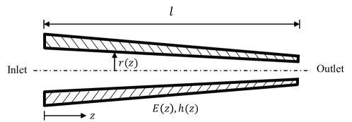
Figure 2: Schematic of a tapered artery model with variable wall elasticity and thickness.

We model the artery as a tapered axisymmetric tube of length $l$, as shown in figure 2. The model has spatially distributed lumen (inner) radius $r(z)$, modulus of elasticity $E(z)$ and wall thickness $h(z)$, where $z$ is the axial coordinate. Following the work of Papadakis (2011), we assume a linear tapering and the change of lumen radius along $z$ is given by

$$r(z)=r_{0}-bz,$$ (3)

where $r_{0}$ is the radius at the inlet and $b$ is a constant that characterizes the degree of tapering. For arteries, tapering is usually very mild and the maximum of $b$ is around 0.026 (Segers and Verdonck, 2000). The blood is assumed to be incompressible. Starting from the mass and momentum conservations, the following classical 1D equations in the cylindrical coordinate system can be derived for the current model under the assumption that the axial displacement is negligible; there is no flow through the lumen wall along $z$ direction; and velocity and pressure are uniform in the cross section (Sherwin et al., 2003; van de Vosse and Stergiopulos, 2011; Figueroa et al., 2017)

$$\frac{\partial A}{\partial t}+\frac{\partial(Av)}{\partial z}&=0,\\ \frac{\partial v}{\partial t}+v\frac{\partial v}{\partial z}+\frac{1}{\rho}\frac{\partial p}{\partial z}=\frac{f}{\rho A}.$$ (4)

Here, $A$ is the area of the cross section; $f$ is the frictional force per unit length; $v$ and $p$ are the cross-sectionally averaged axial velocity and pressure, respectively.

To close this 1D model, we need an extra equation to describe the fluid-structure interaction between blood flow and vessel wall. This is achieved by adopting the tube-law (Sherwin et al., 2003; Alastruey et al., 2011; Papadakis, 2011)

$$p=p_{ext}+\frac{4Eh}{3r^{2}}u_{r},$$ (5)

where $p_{ext}$ is the constant external pressure and $u_{r}$ is the radial displacement of the vessel wall. It is worth noting that equation 5 is derived assuming small displacement ($u_{r}\ll r$) and the vessel wall to be incompressible, linear elastic, thin-walled and longitudinally tethered (Sherwin et al., 2003). This set of equations 4, 5 have been widely used in numerical study of pulse wave propagation in arteries with tapering and variable wall properties (Sherwin et al., 2003; Alastruey et al., 2011; van de Vosse and Stergiopulos, 2011; Figueroa et al., 2017).

Equations 4 and 5 form the governing equations in $(A,v,p)$ form. They are recast to $(v_{r},v,p)$ form for easier manipulation in this study, which is achieved by noting that $\partial A/\partial t\approx 2\pi rv_{r}$ under the small displacement assumption. $v_{r}$ is the radial velocity at the fluid-structure interface. Following the findings from previous work (Sherwin et al., 2003; Reymond et al., 2009), the nonlinear term and viscous term have secondary contribution to the momentum conservation and thus are omitted from equation 4b. To sum up, the governing equations utilized in this study are as follows

$$r\frac{\partial v}{\partial z}+2v_{r}+2\frac{\partial r}{\partial z}v&=0\\ \frac{\partial v}{\partial t}+\frac{1}{\rho}\frac{\partial p}{\partial z}=0\\ \frac{\partial p}{\partial t}-\frac{4Eh}{3r^{2}}v_{r}=0$$ (6)

In this study, we focus on arteries with medium to large sizes. Based on the discussion in section 1, we assume that wall properties follow the general form $Eh=\beta r^{\alpha}$ and limit the study to cases with $\alpha=0,~{}1~{}\text{or}~{}2$ to facilitate discussion.

2.2 Boundary conditions

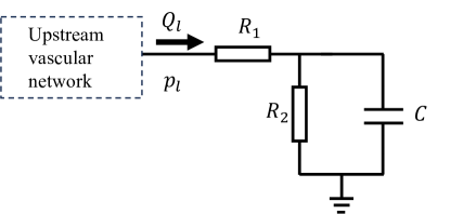
Figure 3: The RCR boundary condition at the outlet. $C$ is the vascular compliance. $R_{1}$, $R_{2}$ are the proximal and distal resistance, respectively.

Proper boundary conditions are required to form a well-posed problem together with the governing equations. At the inlet, a commonly adopted boundary condition is a prescribed velocity profile $v_{in}(t)$ from in vivo measurements

$$v_{0}(t)=v(0,t)=v_{in}(t).$$ (7)

Due to the pulsatile nature of the cardiovascular flow, $v_{in}(t)$ is usually periodic.

The outlet boundary condition represents the effect of downstream vascular networks on the current section, and it plays an important role in capturing the correct characteristics of pulse wave propagation. The downstream effect is usually modeled using lumped parameter models, and the RCR model (three-element Windkessel model, see figure 3) is one of the most popular choices (Westerhof et al., 2009). This model is composed of the vascular compliance $C$, the proximal resistance $R_{1}$ and the distal resistance $R_{2}$. These parameters can be tuned to match the physiological condition of a patient. The RCR boundary condition at the outlet ($x=l$) is governed by the following ordinary differential equation (ODE)

$$\frac{\mathrm{d}p_{l}}{\mathrm{d}t}+\frac{p_{l}}{CR_{2}}=\frac{\left(R_{1}+R_{2}\right)}{CR_{2}}Q_{l}+R_{1}\frac{\mathrm{d}Q_{l}}{\mathrm{d}t},$$ (8)

where flow rate $Q_{l}=\pi r_{l}^{2}v_{l}$, and $p_{l}$ and $v_{l}$ are average pressure and axial velocity at the outlet, respectively.

3 Analytic solution

In this section, we present the closed-form solution to the problem. Solution for a single frequency mode is first derived, and then the time domain solution is obtained by the superposition of all frequency modes. Finally, the solution is validated with 3D numerical simulations.

3.1 Solution for a single frequency mode

To solve the governing equations 6(a-c) with frequency domain analysis, we assume $p(z,t)=P(z)e^{\text{i}\omega t}$ and $v(z,t)=V(z)e^{\text{i}\omega t}$, respectively. Replace $v_{r}$ in equation 6a with equation 6c and replace $Eh$ with $\beta r^{\alpha}$, we end up with the following equations in the frequency domain

$$\text{i}\omega\frac{3r^{2-\alpha}}{2\beta}P+r\frac{\mathrm{d}V}{\mathrm{d}z}-2bV=0,\\ \text{i}\omega V+\frac{1}{\rho}\frac{\mathrm{d}P}{\mathrm{d}z}=0.$$ (9)

Accordingly, the boundary conditions are transformed into the following form

$$v(0,t)&=V_{in}e^{\text{i}\omega t}\\ p(l,t)=Z_{l}V_{l}e^{\text{i}\omega t}$$ (10)

where

$$Z_{l}=\frac{\left(R_{1}+R_{2}+\text{i}\omega R_{1}R_{2}C\right)\pi r_{l}^{2}}{1+\text{i}\omega CR_{2}}$$ (11)

is the impedance of the RCR boundary.

Substitute the pressure in equation 9b with equation 9a and change the partial derivative of $z$ to that of $r$ following the linear tapering relation

$$\frac{\mathrm{d}}{\mathrm{d}z}=-b\frac{\mathrm{d}}{\mathrm{d}r}\quad,\frac{\mathrm{d}^{2}}{\mathrm{d}z^{2}}=b^{2}\frac{\mathrm{d}^{2}}{\mathrm{d}r^{2}}.$$ (12)

We obtain a second-order ODE of $V(r)$

$$r^{2}\frac{\mathrm{d}^{2}V}{\mathrm{d}r^{2}}+(\alpha+1)r\frac{\mathrm{d}V}{\mathrm{d}r}+\left[\frac{3\rho\omega^{2}}{2\beta b^{2}}r^{3-\alpha}-(4-2\alpha)\right]V=0.$$ (13)

With the following transformation

$$y=r^{\frac{\alpha}{2}}V,\quad\varepsilon=\sqrt{\frac{6\rho}{\beta}}\frac{\omega}{b(3-\alpha)}r^{\frac{3-\alpha}{2}},\quad\nu=\frac{4-\alpha}{3-\alpha},$$

this ODE can be rewritten into the standard Bessel equation of order $\nu$ in $y(\varepsilon)$

$$\varepsilon^{2}\frac{\mathrm{d}^{2}y}{\mathrm{d}\varepsilon^{2}}+\varepsilon\frac{\mathrm{d}y}{\mathrm{d}\varepsilon}+(\varepsilon^{2}-\nu^{2})y=0.$$ (14)

Therefore, equation 13 has the following general solution (Bowman, 2012)

$$V=r^{-\frac{\alpha}{2}}\left[c_{1}J_{\nu}(\varepsilon)+c_{2}Y_{\nu}(\varepsilon)\right]$$ (15)

where $J_{\nu}$ and $Y_{\nu}$ are Bessel functions of the first and second kind, and $c_{1}$ and $c_{2}$ are undetermined constants. Pressure can be easily obtained from equation 9a

$$P=-\text{i}\sqrt{\frac{2\rho\beta}{3r}}\left[c_{1}J_{\nu-1}(\varepsilon)+c_{2}Y_{\nu-1}(\varepsilon)\right].$$ (16)

Since $V$ and $P$ satisfy the RCR boundary condition at the outlet, we get $c_{1}=Fc_{2}$, where

$$F=-\frac{\text{i}Z_{l}r_{l}^{\frac{1-\alpha}{2}}Y_{\nu}\left(\varepsilon_{l}\right)-BY_{\nu-1}\left(\varepsilon_{l}\right)}{\text{i}Z_{l}r_{l}^{\frac{1-\alpha}{2}}J_{\nu}\left(\varepsilon_{l}\right)-BJ_{\nu-1}\left(\varepsilon_{l}\right)}$$ (17)

with $B=\sqrt{2\rho\beta/3}$. Taking the inlet boundary condition into consideration, it is solved that

$$c_{1}=V_{in}r_{0}^{\frac{\alpha}{2}}\frac{F}{FJ_{\nu}\left(\varepsilon_{0}\right)+Y_{\nu}\left(\varepsilon_{0}\right)},\quad c_{2}=V_{in}r_{0}^{\frac{\alpha}{2}}\frac{1}{FJ_{\nu}\left(\varepsilon_{0}\right)+Y_{\nu}\left(\varepsilon_{0}\right)}.$$ (18)

To sum up, the analytic solution for a single frequency mode is

$$&V(z,\omega)=V_{in}\left(\frac{r}{r_{0}}\right)^{-\frac{\alpha}{2}}\frac{I_{v}(\varepsilon)}{I_{v}(\varepsilon_{0})},\\ P(z,\omega)=-\text{i}BV_{in}\left(\frac{r}{r_{0}^{\alpha}}\right)^{-\frac{1}{2}}\frac{I_{p}(\varepsilon)}{I_{v}(\varepsilon_{0})},$$ (19)

with $F$ being defined by equation 17 and

$$I_{p}(\varepsilon)=FJ_{\nu-1}(\varepsilon)+Y_{\nu-1}(\varepsilon),\quad I_{v}(\varepsilon)=FJ_{\nu}(\varepsilon)+Y_{\nu}(\varepsilon),$$

$$B=\sqrt{\frac{2\rho\beta}{3}},\quad\varepsilon=\sqrt{\frac{6\rho}{\beta}}\frac{\omega}{b(3-\alpha)}r^{\frac{3-\alpha}{2}}.$$

Setting $\alpha=0$ in equation 19 results in a solution that is similar to the one obtained by Papadakis (2011), which is for a tapered vessel with uniform wall properties. They are all expressed in Bessel functions of order $4/3$ and $1/3$. But differences exist as they are derived under different coordinate systems and complicated boundary conditions are considered in the current study.

3.2 Analytic solution in time domain

Through the discussion in section 3.1, it can be seen that the governing equations and the boundary conditions are all linear with regard to the primary variables. Therefore, the velocity and pressure solutions correspond to an arbitrary periodic inlet velocity profile can be obtained by the superposition of all frequency modes. An inlet velocity profile with period $T$ can be expanded into Fourier series

$$v_{in}(t)=\sum\limits_{n=-\infty}^{\infty}V_{n}^{in}e^{\text{i}\omega_{n}t}$$ (20)

where

$$V_{n}^{in}=\frac{1}{T}\int_{0}^{T}v_{in}(t)e^{-\text{i}\omega_{n}t}dt,\quad\omega_{n}=2\pi n/T.$$

The same operation can be carried out for the velocity and pressure solutions

$$v(z,t)=\sum\limits_{n=-\infty}^{\infty}V_{n}(z)e^{\text{i}\omega_{n}t},\quad p(z,t)=\sum\limits_{n=-\infty}^{\infty}P_{n}(z)e^{\text{i}\omega_{n}t}.$$ (21)

For $n>0$, the expressions for $V_{n}(z)$ and $P_{n}(z)$ are provided by equation 19, while $n=0$ corresponds to the steady flow solution, which is governed by the following equations

$$r\frac{\mathrm{d}V_{0}}{\mathrm{d}z}+2\frac{\mathrm{d}r}{\mathrm{d}z}V_{0}&=0,\\ V_{0}\frac{\mathrm{d}V_{0}}{\mathrm{d}z}+\frac{1}{\rho}\frac{\mathrm{d}P_{0}}{\mathrm{d}z}=0.$$ (22)

Note that the nonlinear term is included here, which we find to improve the accuracy of the pressure prediction. Combining with the boundary conditions, we can obtain the steady state solution as

$$&V_{0}(z)=V_{0}^{in}\frac{r_{0}^{2}}{r^{2}},\\ P_{0}(z)=V_{0}^{in}\pi r_{0}^{2}(R_{1}+R_{2})+\frac{1}{2}\rho\left(V_{0}^{in}\frac{r_{0}^{2}}{r_{l}^{2}}\right)^{2}-\frac{1}{2}\rho\left(V_{0}^{in}\frac{r_{0}^{2}}{r^{2}}\right)^{2}.$$ (23)

Equation 23a is a direct result of mass conservation, while equation 23b is essentially the Bernoulli equation. The first term on the right hand side of equation 23b represents the outlet pressure because RCR boundary is reduced to resistance boundary for steady flow, and the second term is the difference in kinetic energy .

Finally, the time domain solution is

$$v(z,t)&=V_{0}(z)+\mbox{Re}\left\{\sum\limits_{n=1}^{\infty}2V_{n}^{in}\left(\frac{r}{r_{0}}\right)^{-\frac{\alpha}{2}}\frac{I_{v}(\varepsilon)}{I_{v}(\varepsilon_{0})}e^{\text{i}\omega_{n}t}\right\},\\ p(z,t)=P_{0}(z)+\mbox{Re}\left\{\sum\limits_{n=1}^{\infty}-\text{i}2BV_{n}^{in}\left(\frac{r}{r_{0}^{\alpha}}\right)^{-\frac{1}{2}}\frac{I_{p}(\varepsilon)}{I_{v}(\varepsilon_{0})}e^{\text{i}\omega_{n}t}\right\}.$$ (24)

In all cases presented in this paper, we retain the first 20 terms of the series. It has been confirmed that any further increase in $n$ beyond 20 results in negligible improvement to the solution.

3.3 Validation of the analytic solution

Wall properties
$Eh(g\cdot s^{-2})$	$\beta=5.94\times 10^{5},\alpha=1$
Poisson’s ratio	0.5
$\rho_{s}(g\cdot cm^{-3})$	1.0
Fluid properties
$\mu(g\cdot cm^{-1}\cdot s^{-1})$	0.04
$\rho(g\cdot cm^{-3})$	1.06
Vessel geometry
$r_{0}(cm)$	0.4
$r_{l}(cm)$	0.2
$l(cm)$	12.6
Boundary conditions
Inlet	Prescribed flow rate with $T=1.1s$
Outlet	$R_{1},R_{2}\left(g\cdot{cm}^{-4}\cdot s^{-1}\right):6854.8,14330$
	$C\left(g^{-1}\cdot{cm}^{4}\cdot s^{2}\right):1.7529\times 10^{-5}$

Table 1: Parameters of tapered carotid artery model.

Flow through a tapered carotid artery model with the same geometric configuration as figure 2 is used to validate the analytic solution. All relevant parameters are summarized in table 1. The analytic solution is compared with a 3D FSI simulation using coupled momentum method (CMM) (Figueroa et al., 2006), which is implemented in the open-source software svFSI (Zhu et al., 2022). CMM has recently been rigorously verified with Womersley’s deformable wall analytical solution (Filonova et al., 2020). The mesh resolution and the time step size follow the same settings as in Xiao et al. (2014).

We quantify the differences between the analytic solution and the 3D simulation results using the following errors

$$\eta_{P,avg}=\frac{1}{N}\sum\limits_{i=1}^{N}\left|\frac{P_{i}^{a}-P_{i}^{c}}{P_{i}^{c}}\right|, \eta_{Q,avg}=\frac{1}{N}\sum\limits_{i=1}^{N}\left|\frac{Q_{i}^{a}-Q_{i}^{c}}{max_{j}\left(Q_{j}^{c}\right)}\right|,$$

$$\eta_{P,max}=max_{i}\left|\frac{P_{i}^{a}-P_{i}^{c}}{P_{i}^{c}}\right|, \eta_{Q,max}=max_{i}\left|\frac{Q_{i}^{a}-Q_{i}^{c}}{max_{j}\left(Q_{j}^{c}\right)}\right|.$$

$N$ is the number of sampling time points and is set to 125 here. $P_{i}^{a}$ and $Q_{i}^{a}$ are the pressure and flow rate calculated analytically, while $P_{i}^{c}$ and $Q_{i}^{c}$ are the mean pressure and flow rate on the cross section from CMM. $\eta_{avg}$ reports the average relative error, while $\eta_{max}$ is the maximum relative error. In order to avoid dividing by small values in flow rate comparison, we divide the errors by the maximum flow rate for normalization (Xiao et al., 2014).

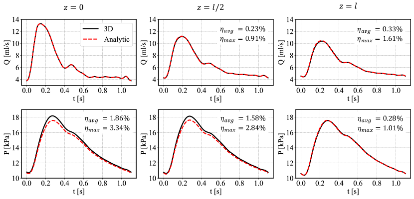
Figure 4: Comparison between the analytic solutions and 3D simulation results for the tapered carotid with $\alpha=1$. Top row is the flow rate comparison, and bottom row is the pressure comparison.

The comparison of flow rate and pressure at the inlet, mid-section and outlet of the carotid artery model is summarized in figure 4. Since the flow rates are prescribed at the inlet in both cases, they match exactly. Though errors in flow rate increase slowly towards the outlet, the values predicted by the analytic solution are still in excellent agreement with the 3D simulation results, with the maximum error being $1.61\%$ at the outlet. Moreover, the average relative errors of pressure never exceed $1.86\%$, and the maximum relative errors remain under $3.4\%$. Contrary to flow rate, the errors of pressure decrease gradually from the inlet to the outlet. Since the RCR boundary condition is given at the outlet, the pressure is directly calculated from the flow rate there. Towards the inlet, the errors caused by omitting the fluid viscosity and nonlinear term likely accumulate to cause the slightly larger difference in pressure values.

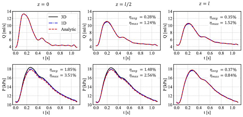
Figure 5: Comparison between the analytic solutions and 1D, 3D simulation results for the tapered carotid with uniform wall properties. 1D results are extracted from Xiao et al. (2014) and $\alpha=0$, $\beta=2.1\times 10^{5}$.

In addition to the 3D FSI simulation results, the analytic solutions are also compared with the results reported in Xiao et al. (2014), wherein they used 1D numerical simulations to study the pulse wave propagation in the same geometry but with uniform wall properties (see figure 5). Overall, results predicted by the analytic solution are in great agreement with those from numerical simulations with either uniform or variable wall properties.

4 Theoretical analysis of pulse wave propagation

In this section, the analytic solution is used to analyze the effect of wall properties on pulse wave propagation in flexible tubes. As shown in figure 6a, we focus on cases where $\alpha=0,$ $1$ and $2$. $Eh$ value is kept the same at the inlet of all three cases.

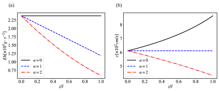
Figure 6: Distribution of (a) wall properties and (b) wave velocity along the carotid artery model. Here, $\beta=2.376\times 10^{5}/r_{0}^{\alpha}$ so that all three cases have the same $Eh$ value at the inlet. Other parameters are from table 1.

4.1 Wave propagation velocity

The governing equation 6 can be rewritten into the following form

$$\frac{\partial\boldsymbol{U}}{\partial t}+\mathsfbi{A}\frac{\partial\boldsymbol{U}}{\partial z}=\mathsfbi{B}\boldsymbol{U}$$ (25)

where

$$\boldsymbol{U}=\left[\begin{array}[]{l}p\\ v\end{array}\right],\quad\mathsfbi{A}=\left[\begin{array}[]{cc}0&\frac{2Eh}{3r}\\ \frac{1}{\rho}&0\end{array}\right],\quad\mathsfbi{B}=\left[\begin{array}[]{cc}0&\frac{4Ehb}{3r^{2}}\\ 0&0\end{array}\right].$$ (26)

This apparently forms a system of hyperbolic equations, and the wave propagation velocity can be obtained by solving for the eigenvalues of matrix $\mathsfbi{A}$ (Papadakis, 2011; Alastruey et al., 2012), which is

$$c=\pm\sqrt{\frac{2Eh}{3\rho r}}=\pm\sqrt{\frac{2\beta}{3\rho}}r^{\frac{\alpha-1}{2}}.$$ (27)

It can be seen from figure 6 that as $\alpha$ increases, the $Eh$ value decreases at the same axial location of the model. On the other hand, wave velocity increases along the model when $\alpha=0$, while it decreases for $\alpha=2$. $\alpha=1$ is a special case where the wave velocity remains constant. It is worth noting that the wave velocity expressed in $Eh$ is consistent with the well-known Moens-Korteweg equation (Korteweg, 1878; Moens, 1878; Alastruey et al., 2012), which is derived for straight tubes without tapering. Papadakis (2011) derived the wave velocity for a tapered vessel with uniform wall properties using spherical coordinates. The result included a correction term of second order $O(\theta^{2})$ due to tapering, where $\theta=\arctan(b)$. In arterial systems, this correction term is negligible as the tapering angle is usually less than $1.5^{\circ}$.

4.2 Input Impedance

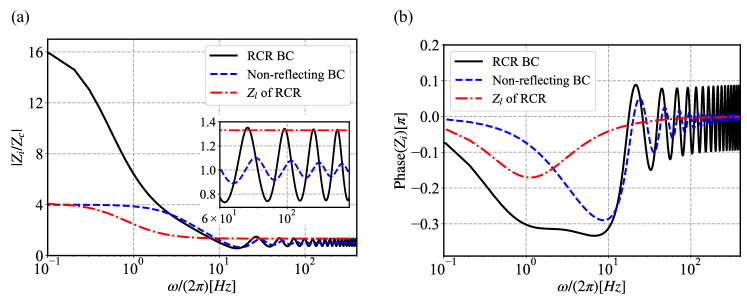
Figure 7: (a) Magnitude and (b) phase of the input impedance of the tapered carotid artery model. Here, the magnitude is normalized by the characteristic impedance at the inlet. Parameters from table 1 are used.

With the wave velocity, the characteristic impedance can be expressed as $Z_{c}=\rho c$ (Westerhof et al., 2010). It is a representation of the local wave transmission characteristic of the system without considering any reflections.

Moreover, based on the analytic solution 19, we have

$$P=-\text{i}Br^{\frac{\alpha-1}{2}}\frac{I_{p}(\varepsilon)}{I_{v}(\varepsilon)}V=-\text{i}\rho c\frac{I_{p}(\varepsilon)}{I_{v}(\varepsilon)}V=ZV,$$ (28)

where $Z$ is the impedance (Westerhof et al., 2010). $Z$ is a function of both axial location and frequency, while $Z_{c}$ is a function of axial location only. $Z$ evaluated at $z=0$ is referred to as the input impedance $Z_{i}$. Compared with the characteristic impedance, the additional coefficient $-\text{i}I_{p}/I_{v}$ in $Z_{i}$ measures the influence of the reflected waves caused by tapering, wall property change and outlet boundary condition. If $I_{p}/I_{v}=\text{i}$, the input impedance is equal to the characteristic impedance, i.e. there is no wave reflection from downstream of the inlet. This is discussed in detail below.

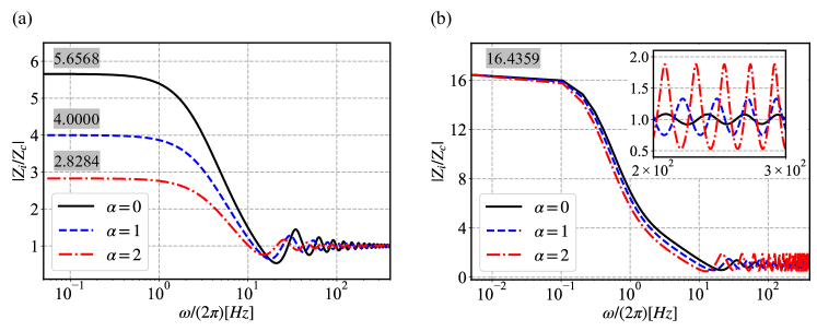
Figure 8: Magnitude of the input impedance of the tapered carotid artery model with different $\alpha$. (a) Non-reflecting boundary condition is employed; (b) RCR boundary condition is employed. The shaded numbers are the asymptotic values as $\omega\rightarrow 0$ predicted by equation 31.

The change of input impedance with frequency is of great interest in cardiovascular research (Murgo et al., 1980; Taylor, 1966). Figure 7 plots the input impedance of the carotid artery model with $\alpha=1$. Two different boundary conditions are considered here

$$Z_{l}&=\rho c_{l},\quad\quad\quad\quad\quad\quad\quad\quad\quad\quad\mathrm{for\ non-reflecting\ boundary};\\ Z_{l}=\frac{\left(R_{1}+R_{2}+\text{i}\omega R_{1}R_{2}C\right)\pi r_{l}^{2}}{1+\text{i}\omega CR_{2}},\quad\mathrm{for\ physiological\ RCR\ boundary}.$$ (29)

Here, $c_{l}$ is the wave velocity at the outlet. It is worth emphasizing that $Z_{i}$ is normalized by local characteristic impedance, which is $Z_{c}=\rho c_{0}$. For the case with non-reflecting boundary condition, the input impedance at low-frequency band is almost four times that of the local characteristic impedance even without any reflection from the outlet. This disparity can be attributed to the constant reflection of the forward flow due to tapering as well the change in wall properties. As the frequency increases, the input impedance decreases and eventually approaches the local characteristic impedance. The phase of the input impedance with non-reflecting boundary also converges to zero as the frequency increases. This indicates that tapering mainly affects the waves with long wavelength, while waves with short wavelength behave as if tapering does not exist. For the case with RCR boundary condition, the input impedance is much higher than the local characteristic impedance at low-frequency band and is nearly four times of the non-reflecting case. The outlet impedance $Z_{l}$ of RCR boundary is also plotted in figure 7. It is clear that RCR boundary induces a much greater increment in the magnitude of the input impedance than its own magnitude. As the frequency increases, the input impedance of the RCR case does not reduce to zero, but rather oscillates around $Z_{c}$ as is shown in both the magnitude and the phase plots. Therefore, the inclusion of a physiologically accurate outlet boundary condition is very crucial in the study of the input impedance of arteries.

The effect of $\alpha$ is shown in figure 8. For cases with non-reflecting outlet, the behavior of the input impedance at high-frequency band is unaffected by the profile of the wall properties, approaching the local characteristic impedance asymptotically. As is shown in appendix A, when $\omega\rightarrow\infty$, $\varepsilon\rightarrow\infty$. Substitute $Z_{l}=\rho c_{l}$ into equation 44, we have $Z_{i}\approx\rho c_{0}$ when $\omega\rightarrow\infty$. Otherwise, when the RCR boundary condition is employed, the input impedance oscillates around the local characteristic impedance at high frequencies. From equation 44, it can be shown that as $\omega\rightarrow\infty$, we have

$$\bigg{|}\frac{Z_{i}}{Z_{c}}\bigg{|}_{max}=\max\left\{\frac{R_{1}\pi r_{l}^{2}}{\rho c_{l}},\frac{\rho c_{l}}{R_{1}\pi r_{l}^{2}}\right\},\quad\text{and}\quad\bigg{|}\frac{Z_{i}}{Z_{c}}\bigg{|}_{min}=\min\left\{\frac{R_{1}\pi r_{l}^{2}}{\rho c_{l}},\frac{\rho c_{l}}{R_{1}\pi r_{l}^{2}}\right\}~{}\text{at}~{}z=0.$$ (30)

The accuracy of this asymptotic relation is confirmed numerically. It is clear that the oscillation amplitude is determined by the proximal resistance $R_{1}$ and $\alpha$.

On the other hand, as the frequency decreases, the input impedance converges to the same value regardless of $\alpha$ when RCR boundary is used, while its value decreases as the $\alpha$ value increases when non-reflecting boundary is used. It can be proven (see appendix B) that as $\omega\rightarrow 0$

$$\frac{Z_{i}}{Z_{c}}\bigg{|}_{z=0}&\approx\left(\frac{r_{0}}{r_{l}}\right)^{\frac{5-\alpha}{2}},\quad\mathrm{for\ non-reflecting\ boundary},\\ \frac{Z_{i}}{Z_{c}}\bigg{|}_{z=0}\approx\frac{\pi r_{0}^{2}}{\rho c_{0}}(R_{1}+R_{2}),\quad\mathrm{for\ physiological\ RCR\ boundary}.$$ (31)

Equation 31a clearly shows that $Z_{i}$ is determined by tapering and wall properties jointly, while equation 31b shows that RCR boundary condition is the determining factor when it is present. The normalized input impedances predicted by these two equations are also listed in figure 8. Compared with values evaluated numerically at $5\times 10^{-3}Hz$, the maximum relative difference is less than 0.1%, affirming the accuracy of the asymptotic analysis.

The input impedance predicted by the current model (figure 8b) are in qualitative agreement with in vivo measurements (Nichols et al., 1977; Murgo et al., 1980). Murgo et al. (1980) measured the aortic input impedance in 18 healthy man and noticed the same trend that $|Z_{i}|$ achieved its maximum at low-frequency, decreased sharply and started to oscillate between $6-8Hz$. Unlike the current study, the oscillation amplitude decreased with increasing frequency due to viscous damping in the arterial wall.

4.3 Wave reflection

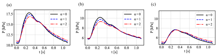
Figure 9: Pressure waves at $z=l/2$ of the tapered carotid artery model with RCR boundary condition and different $\alpha$. (a) Total pressure wave; (b) forward wave; (c) backward wave. The $y$-axis of the forward and backward waves is set to the same range to facilitate comparison.

Tapering, wall property variation and outlet impedance all cause pulse wave reflections. The pressure wave can be separated into forward and backward components using (Westerhof et al., 1972)

$$p_{f,b}=\frac{1}{2}(p\pm\rho cv).$$ (32)

Pressure waves at mid-section and its components are compared in figure 9. As the $\alpha$ value increases, the artery becomes more compliant, which leads to a decrease in the pulse pressure (difference between the maximum and minimum). This decrease is a combined result of an increase in diastolic pressure (minimum) and a decrease in systolic pressure (maximum). From figures 9b and c, it is clear that the forward wave is mostly responsible for the reduction of peak value while the diastolic value is mostly raised by the backward wave. We can also observe a slight temporal shift of the peak pressure value as $\alpha$ changes due to the change in pulse wave velocity.

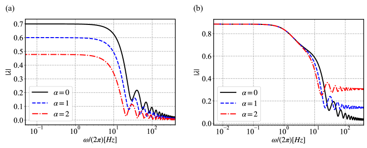
Figure 10: Reflection coefficient at the inlet of the tapered carotid artery model with different $\alpha$. (a) Non-reflecting boundary condition is employed; (b) RCR boundary condition is employed.

Equation 32 can also be applied to each frequency component and we have

$$P_{f} =\frac{1}{2}V_{in}Br_{0}^{\frac{\alpha}{2}}r^{-\frac{1}{2}}\left(-\frac{I_{p}(\varepsilon)}{I_{v}\left(\varepsilon_{0}\right)}\text{i}+\frac{I_{v}(\varepsilon)}{I_{v}\left(\varepsilon_{0}\right)}\right),$$ (33)

$$P_{b} =\frac{1}{2}V_{in}Br_{0}^{\frac{\alpha}{2}}r^{-\frac{1}{2}}\left(-\frac{I_{p}(\varepsilon)}{I_{v}\left(\varepsilon_{0}\right)}\text{i}-\frac{I_{v}(\varepsilon)}{I_{v}\left(\varepsilon_{0}\right)}\right).$$ (34)

The reflection coefficient can be defined as (Reymond et al., 2009; Westerhof et al., 2010)

$$\lambda=\frac{P_{b}}{P_{f}}=\frac{\text{i}I_{p}/I_{v}+1}{\text{i}I_{p}/I_{v}-1}=\frac{Z_{i}/Z_{c}-1}{Z_{i}/Z_{c}+1}$$ (35)

Here, $\lambda$ is complex indicating the phase difference between the forward and backward waves. From figure 10, we can see that the behaviors of the reflection coefficient are mostly similar to the input impedance in figure 8. One interesting trend is that at high-frequency range with RCR boundary, the reflection coefficient increases with $\alpha$ indicating a growing relative contribution from the backward waves.

5 Application of the analytic solution

Though developed based on an idealized model, equation 24 can be applied to complex, patient-specific cases. Here we demonstrate the application of the analytic solution to a patient-specific aorta and compare with the results from 3D numerical simulations using CMM.

5.1 Analytic solution for bifurcation

The analytic solution presented in this study can be extended to complex models with multiple outlets by decomposing the model into simple blocks that are easier to solve. Similar strategies are adopted in distributed lumped parameter models (Mirramezani and Shadden, 2022) and 1D models (van de Vosse and Stergiopulos, 2011). One of the most common building blocks in an arterial network is the bifurcation. Figure 11a shows a typical bifurcation where a parent vessel (labeled $a$) is connected to two daughter vessels (labeled $b$ and $c$). Each vessel in figure 11b can be solved with the analytic solution given the proper inlet and outlet boundary conditions, and their solutions are related by the following conditions at the junction (Olufsen, 1999)

$$&P_{l}^{a}=P_{0}^{b}=P_{0}^{c},\\ V_{l}^{a}\pi\left(r_{l}^{a}\right)^{2}=V_{0}^{b}\pi\left(r_{0}^{b}\right)^{2}+V_{0}^{c}\pi\left(r_{0}^{c}\right)^{2}.$$ (36)

Here, the subscripts $0$ and $l$ represent the inlet and outlet of each vessel. For vessel $a$, velocity is prescribed at the inlet and a proper outlet boundary condition, $Z_{l}^{a}$, is required to obtain its solution. Divide equation 36b by equation 36a, we get

$$\frac{\pi\left(r_{l}^{a}\right)^{2}}{Z_{l}^{a}}=\frac{\pi\left(r_{0}^{b}\right)^{2}}{Z_{0}^{b}}+\frac{\pi\left(r_{0}^{c}\right)^{2}}{Z_{0}^{c}}.$$ (37)

The outlet impedance of the vessel $a$ is determined by the input impedances of vessel $b$ and $c$. If vessel $b$ and $c$ are terminal vessels, i.e. they are connected to RCR models, $Z_{0}^{b}$ and $Z_{0}^{c}$ can be determined explicitly through equation 28. Then, $Z_{l}^{a}$ is readily available through equation 37, and the velocity and pressure along vessel $a$ can be obtained. It is worth noting that equation 37 essentially describes that the input impedance of vessel $b$ and $c$ are connected in parallel to form the outlet impedance of vessel $a$.

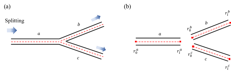
Figure 11: (a) Schematic of a bifurcation with splitting flow. (b) Decomposition of the bifurcation into three individual vessels. Here, the subscripts $0$ and $l$ represent the inlet and outlet of each vessel, respectively.

For vessel $b$, once the pressure value at its inlet is known, the inlet velocity of vessel $b$ can be obtained from equation 19b. Therefore, the solution in this vessel is written as

$$V^{b}(z) =\text{i}\frac{P_{l}^{a}}{B^{b}}\left(r_{0}^{b}\right)^{\frac{1}{2}}\left(r^{b}\right)^{-\frac{\alpha}{2}}\frac{I_{v}\left(\varepsilon^{b}\right)}{I_{p}\left(\varepsilon^{b}_{0}\right)}$$ (38)

$$P^{b}(z) =P_{l}^{a}\left(\frac{r_{0}^{b}}{r^{b}}\right)^{\frac{1}{2}}\frac{I_{p}\left(\varepsilon^{b}\right)}{I_{p}\left(\varepsilon^{b}_{0}\right)}$$ (39)

The same calculation can be carried out for vessel $c$. This procedure can be expanded to multiple layers of bifurcations as well as junctions with more than two daughter vessels.

Similar to the current study, Flores et al. (2016) proposed an analytic solution based on the generalized Darcy’s elastic model in the frequency domain and successfully applied it to model blood flow in complex arterial networks. However, the vessel was assumed to be cylindrical and to have uniform material properties. The tapering and material variation in a large network were modeled in a discrete manner by dividing long vessels into segments. Pressure values at segment ends were treated as unknown variables and were obtained by solving a matrix system constructed from these segments. In the current study, tapering and material changes are built into the analytic solution. The solution process described above is much simpler and can be considered a special case of the matrix-based method when the network only contains splitting junctions.

5.2 Application to patient-specific aorta

We use a patient-specific aorta model to demonstrate the accuracy and effectiveness of the analytic solution. The model is from an open source dataset (BodyParts3D, 2011) and is shown in figure 12. It includes the aorta and three main branches and is broken into individual sections indicated by the dashed lines for analytic modeling. The parameters used in each section are also listed in the figure. The vessel length $l$ is defined as the length of the curved centerline. The variation of the material properties follows the linear relation in figure 1, i.e. $Eh=\beta r$ with $\beta=5.94\times 10^{5}g\cdot cm^{-1}\cdot s^{-2}$. A pulsatile velocity profile with $T=0.9s$ is prescribed at AAo, and RCR boundary conditions are applied at all of the outlets. In CMM simulations, a grid independence study is carried out and around 0.5 million tetrahedral elements are used to obtained the final results. Based on the Womersley number ($Wo=r\sqrt{2\pi\rho f/\mu}\approx 16$) and the Reynolds number defined with Stokes layer thickness ($Re_{\delta}=\sqrt{2\rho}v_{max}/\sqrt{\mu\omega}\approx 195$), the flow has not transitioned to turbulence under the conditions considered here (Merkli and Thomann, 1975; Hino et al., 1976).

The flow rate and pressure at the inlet and outlets are summarized in figure 13. It can be seen that analytic results are in good agreement with numerical results. The pressure distribution is particularly well-matched, as the maximum relative error is maintained below $2\%$ and the average relative error remains under $1\%$. The average relative error of the flow rate is less than $2.4\%$, while the maximum error is higher due to a slight phase difference between these two results. It is worth noting that analytic results can be obtained within 1 second on a desktop equipped with an Intel Core i9-12900K processor, while 3D simulations take approximately 20 minutes per cardiac cycle when run in parallel on 288 Intel Xeon Platinum 9242 cores. Therefore, the analytic solution provides a fast and accurate alternative to 3D simulations in estimating the pressure distribution in this model.

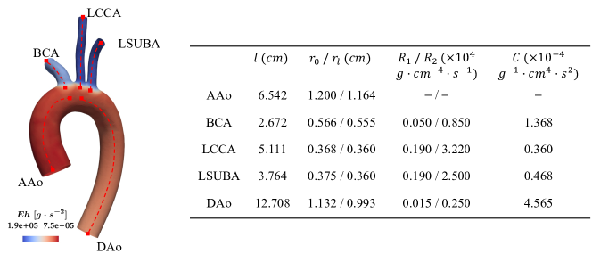
Figure 12: Patient-specific aorta model and the parameters used in the study. The dashed lines indicate all the sections of arteries used in the analytic model. AAo: Ascending Aorta; BCA: Brachiocephalic Artery; LCCA: Left Common Carotid Artery; LSUBA: Left Subclavian Artery; DAo: Descending Aorta.

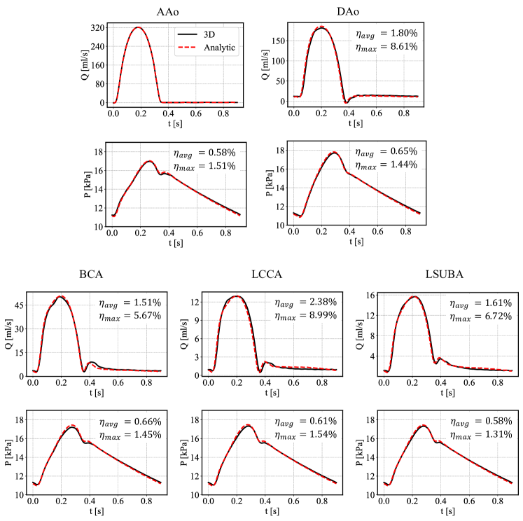
Figure 13: Comparison between the analytic solutions and 3D simulation results for the patient-specific aorta model.

6 Conclusion

In this study, we derive an analytic solution for pulse wave propagation in an arterial model using frequency domain analysis. In addition to tapering, this model also includes variable wall properties that follow the profile $Eh=\beta r^{\alpha}$ and a physiological RCR outlet boundary condition that models the resistance and compliance of the downstream vascular network. This analytic solution is successfully validated against 1D and 3D numerical simulations. Then, it is used to theoretically analyze the wave propagation characteristics in an idealized model. It is confirmed that tapering and variable wall properties can create constant reflections along the path. Our study also demonstrates that wall properties and RCR boundary condition have a significant impact on the wave propagation, and their influences are particularly prominent at the low-frequency range. Even though it is observed in figure 8 that high-frequency components are also affected by these factors, it is essential to approach these findings with caution, as viscous effect is not considered in the current model. Furthermore, it is worth noting that these high-frequency components may not hold significant physiological relevance, given the intrinsic frequency of the cardiac cycle.

Moreover, the analytic solution is applied to rapidly and accurately estimate the pressure distribution in a patient-specific aorta by splitting the model into individual sections and applying the analytic solution to each section. Compared to numerical methods, the analytic solution can be a computationally economical alternative for modeling pulse wave propagation. It also enables theoretical analysis to quantify the influence of different model parameters, such as boundary conditions and material properties, thus allowing for quick tuning of these parameters, which can then be used in 1D and 3D numerical simulations. Additionally, this method is potentially useful for clinical applications such as the estimation of the central pressure from peripheral pressure measurements. Building upon the study by Flores et al. (2021), it is possible to model the pressure wave propagation from the aorta to the brachial artery using the current analytic solution and derive a transfer function between central and brachial pressure.

There are several limitations in the current study. First, the omission of the nonlinear term (except for the steady component) and blood viscosity in the momentum equation leads to the under-estimation of pressure values. Reymond et al. (2009) demonstrated that both effects contributed about single-digit percentages to the predicted pressure value. Given that the errors we observe are of the same order of magnitude, including these effects can potentially improve our results. This is especially important in predicting pulse wave propagation within a long artery network with multiple layers of bifurcations, in which case avoiding error accumulation is of greater importance. Second, the blood vessel is more accurately modeled as a viscoelastic material. Experimental evidences have shown that there is hysteresis between pressure and lumen area (Valdez-Jasso et al., 2009) and the viscoelasticity causes attenuation of pulse waves as they travel downstream (Bessems et al., 2008). Last but not least, the current model cannot be applied directly to diseased arteries such as those with aneurism or stenosis, but can potentially be expanded to model these anomalies (Papadakis and Raspaud, 2019).

Acknowledgements.

The authors thank Dr. Baofang Song for valuable discussions.

Funding.

This work is supported by the National Key Research and Development Program of China (grant nos 2021YFA1000200, 2021YFA1000201) and the National Natural Science Foundation of China (grant no. 12272009). C.Z. also received financial support from Fundamental Research Funds for the Central Universities, Peking University (grant nos 7100604109, 7100604343) and Young Elite Scientists Sponsorship Program by BAST (grant no. BYESS2023025).

Declaration of interests.

The authors report no conflict of interest.

Author ORCIDs.

C. Zhu, https://orcid.org/0000-0002-1099-8893

Appendix A High-frequency limit

When $\omega\rightarrow\infty$, we have $\varepsilon\rightarrow\infty$. For Bessel functions at $\varepsilon\rightarrow\infty$, we have (Abramowitz and Stegun, 1948)

$$J_{\nu}(\varepsilon)\approx\sqrt{\frac{2}{\pi\varepsilon}}\cos\left(\varepsilon-\frac{v}{2}\pi-\frac{\pi}{4}\right),\quad Y_{\nu}(\varepsilon)\approx\sqrt{\frac{2}{\pi\varepsilon}}\sin\left(\varepsilon-\frac{v}{2}\pi-\frac{\pi}{4}\right).$$ (40)

From equation 11, the impedance at the outlet can be simplified to a real value

$$Z_{l}\approx R_{1}\pi r_{l}^{2}.$$ (41)

Define

$$R_{l}=\frac{Z_{l}r_{l}^{\frac{1-\alpha}{2}}}{B}=\frac{Z_{l}}{\rho c_{l}}$$ (42)

and substitute the above equations into equation 17, and we obtain

$$F\approx-\frac{\text{i}R_{l}\sin\left(\varepsilon_{l}-\frac{v}{2}\pi-\frac{\pi}{4}\right)-\cos\left(\varepsilon_{l}-\frac{v}{2}\pi-\frac{\pi}{4}\right)}{\text{i}R_{l}\cos\left(\varepsilon_{l}-\frac{v}{2}\pi-\frac{\pi}{4}\right)+\sin\left(\varepsilon_{l}-\frac{v}{2}\pi-\frac{\pi}{4}\right)}$$ (43)

The normalized input impedance as $\varepsilon\rightarrow\infty$ can be simplified to

$$\frac{Z_{i}}{Z_{c}}\bigg{|}_{z=0} =-\text{i}\frac{I_{p}}{I_{v}}\bigg{|}_{z=0}$$

$$\approx\left[\frac{R_{l}}{R_{l}^{2}\sin^{2}\theta+\cos^{2}\theta}+\text{i}\frac{\left(R_{l}^{2}-1\right)\sin\theta\cos\theta}{R_{l}^{2}\sin^{2}\theta+\cos^{2}\theta}\right]\bigg{|}_{z=0}.$$ (44)

Here, $\theta=\varepsilon_{l}-\varepsilon$. If $Z_{l}=\rho c_{l}$, we have $R_{l}=1$ and $Z_{i}\approx Z_{c}$ at the inlet. If $R_{l}\neq 1$, it can be shown the period of $|Z_{i}/Z_{c}|$ is $\theta=\pi$ and the maximum and minimum are $\max\left\{R_{l},1/R_{l}\right\}$ and $\min\left\{R_{l},1/R_{l}\right\}$, respectively.

Appendix B Low-frequency limit

In the limit $\omega\rightarrow 0$, we have $\varepsilon\rightarrow 0$ and the following relation for Bessel function (Abramowitz and Stegun, 1948)

$$J_{\nu}(\varepsilon)\approx\frac{1}{\Gamma(v+1)}\left(\frac{\varepsilon}{2}\right)^{v},\quad Y_{\nu}(\varepsilon)\approx-\frac{\Gamma(v)}{\pi}\left(\frac{\varepsilon}{2}\right)^{-v}.$$ (45)

Moreover, from equation 11, the impedance at the outlet can be simplified to a real value

$$Z_{l}\approx(R_{1}+R_{2})\pi r_{l}^{2}.$$ (46)

Substitute the above relationships along with equation 42 into equation 17, and we obtain

$$F=\underbrace{-\frac{R_{l}^{2}J_{\nu}Y_{\nu}+J_{\nu-1}Y_{\nu-1}}{R_{l}^{2}J_{\nu}^{2}+J_{\nu-1}^{2}}}_{F_{r}}+\text{i}\underbrace{\frac{R_{l}(J_{\nu-1}Y_{\nu}-J_{\nu}Y_{\nu-1})}{R_{l}^{2}J_{\nu}^{2}+J_{\nu-1}^{2}}}_{F_{i}}.$$ (47)

Note that the Bessel functions are evaluated at $\varepsilon_{l}$ here. From the asymptotic relation in equation 45 and the parameters in table 1, it can be shown that the following equations hold in this study

$$|F_{r}|\ll|F_{i}|,\quad|J_{\nu}Y_{\nu-1}|\ll|J_{\nu-1}Y_{\nu}|.$$

Hence, in the limit of $\varepsilon\rightarrow 0$, we have

$$F\approx\text{i}F_{i},$$ (48)

and

$$F_{i}\approx\frac{R_{l}(J_{\nu-1}Y_{\nu})}{R_{l}^{2}J_{\nu}^{2}+J_{\nu-1}^{2}}\approx-\frac{R_{l}\nu^{2}\Gamma(\nu)^{2}}{\pi}\left[R_{l}^{2}\left(\frac{\varepsilon_{l}}{2}\right)^{2\nu+1}+\nu^{2}\left(\frac{\varepsilon_{l}}{2}\right)^{2\nu-1}\right]^{-1}.$$ (49)

The recursive relation $\Gamma(v+1)=v\Gamma(v)$ is used in the above derivation.

The normalized input impedance as $\varepsilon\rightarrow 0$ can be simplified to

$$\frac{Z_{i}}{Z_{c}}\bigg{|}_{z=0}=-\text{i}\frac{I_{p}}{I_{v}}\bigg{|}_{z=0}\approx F_{i}\frac{J_{\nu-1}}{Y_{\nu}}\bigg{|}_{z=0}.$$ (50)

Further simplify the above equation, we obtain

$$\frac{Z_{i}}{Z_{c}}\bigg{|}_{z=0}\approx R_{l}\left(\frac{\varepsilon_{0}}{\varepsilon_{l}}\right)^{2\nu-1}.$$ (51)

It is verified that the asymptotic equation 51 is valid for both non-reflecting boundary and physiological RCR boundary. In both cases, as $\varepsilon\rightarrow 0$, we have

$$\frac{Z_{i}}{Z_{c}}\bigg{|}_{z=0}&\approx\left(\frac{r_{0}}{r_{l}}\right)^{\frac{5-\alpha}{2}},\quad\mathrm{for\ non-reflecting\ boundary},\\ \frac{Z_{i}}{Z_{c}}\bigg{|}_{z=0}\approx\frac{\pi r_{0}^{2}}{\rho c_{0}}(R_{1}+R_{2}),\quad\mathrm{for\ physiological\ RCR\ boundary}.$$ (52)

where $c_{0}$ is the pulse wave velocity at the inlet. Equation 52b is consistent with the steady state solution (equation 23), neglecting the nonlinear effect.

References

- Safar et al. [2003] Michel E. Safar, Bernard I. Levy, and Harry Struijker-Boudier. Current Perspectives on Arterial Stiffness and Pulse Pressure in Hypertension and Cardiovascular Diseases. Circulation, 107(22):2864–2869, June 2003. ISSN 0009-7322, 1524-4539. doi:10.1161/01.CIR.0000069826.36125.B4.
- van de Vosse and Stergiopulos [2011] Frans N. van de Vosse and Nikos Stergiopulos. Pulse Wave Propagation in the Arterial Tree. Annual Review of Fluid Mechanics, 43(1):467–499, January 2011. ISSN 0066-4189, 1545-4479. doi:10.1146/annurev-fluid-122109-160730.
- Moens [1878] A Isebree Moens. Die pulscurve. Brill, 1878.
- Segers and Verdonck [2000] Patrick Segers and Pascal Verdonck. Role of tapering in aortic wave reflection: Hydraulic and mathematical model study. Journal of Biomechanics, 33(3):299–306, 2000. ISSN 0021-9290. doi:10.1016/S0021-9290(99)00180-3.
- Bessems et al. [2008] David Bessems, Christina G Giannopapa, Marcel CM Rutten, and Frans N van de Vosse. Experimental validation of a time-domain-based wave propagation model of blood flow in viscoelastic vessels. Journal of biomechanics, 41(2):284–291, 2008.
- Korteweg [1878] Diederik Johannes Korteweg. Over voortplantings-snelheid van golven in elastische buizen, volume 1. Van Doesburgh, 1878.
- Womersley [1955] J.R. Womersley. XXIV. Oscillatory motion of a viscous liquid in a thin-walled elastic tube—I: The linear approximation for long waves. The London, Edinburgh, and Dublin Philosophical Magazine and Journal of Science, 46(373):199–221, February 1955. ISSN 1941-5982, 1941-5990. doi:10.1080/14786440208520564.
- Womersley [1957] J R Womersley. Oscillatory Flow in Arteries: The Constrained Elastic Tube as a Model of Arterial Flow and Pulse Transmission. Physics in Medicine and Biology, 2(2):178–187, October 1957. ISSN 0031-9155. doi:10.1088/0031-9155/2/2/305.
- Papadakis [2011] George Papadakis. New analytic solutions for wave propagation in flexible, tapered vessels with reference to mammalian arteries. Journal of Fluid Mechanics, 689:465–488, December 2011. ISSN 0022-1120, 1469-7645. doi:10.1017/jfm.2011.424.
- Alastruey et al. [2011] Jordi Alastruey, Ashraf W. Khir, Koen S. Matthys, Patrick Segers, Spencer J. Sherwin, Pascal R. Verdonck, Kim H. Parker, and Joaquim Peiró. Pulse wave propagation in a model human arterial network: Assessment of 1-D visco-elastic simulations against in vitro measurements. Journal of Biomechanics, 44(12):2250–2258, August 2011. ISSN 0021-9290. doi:10.1016/j.jbiomech.2011.05.041.
- Mynard and Smolich [2015] Jonathan P. Mynard and Joseph J. Smolich. One-Dimensional Haemodynamic Modeling and Wave Dynamics in the Entire Adult Circulation. Annals of Biomedical Engineering, 43(6):1443–1460, June 2015. ISSN 0090-6964, 1573-9686. doi:10.1007/s10439-015-1313-8.
- Charlton et al. [2019] Peter H. Charlton, Jorge Mariscal Harana, Samuel Vennin, Ye Li, Phil Chowienczyk, and Jordi Alastruey. Modeling arterial pulse waves in healthy aging: A database for in silico evaluation of hemodynamics and pulse wave indexes. American Journal of Physiology-Heart and Circulatory Physiology, 317(5):H1062–H1085, November 2019. ISSN 0363-6135, 1522-1539. doi:10.1152/ajpheart.00218.2019.
- Zimmermann et al. [2021] Judith Zimmermann, Michael Loecher, Fikunwa O. Kolawole, Kathrin Bäumler, Kyle Gifford, Seraina A. Dual, Marc Levenston, Alison L. Marsden, and Daniel B. Ennis. On the impact of vessel wall stiffness on quantitative flow dynamics in a synthetic model of the thoracic aorta. Scientific Reports, 11(1):6703, March 2021. ISSN 2045-2322. doi:10.1038/s41598-021-86174-6.
- Atabek and Lew [1966] H.B. Atabek and H.S. Lew. Wave Propagation through a Viscous Incompressible Fluid Contained in an Initially Stressed Elastic Tube. Biophysical Journal, 6(4):481–503, July 1966. ISSN 00063495. doi:10.1016/S0006-3495(66)86671-7.
- Lighthill [2001] James Lighthill. Waves in fluids. Cambridge university press, 2001.
- Flores et al. [2016] Joaquín Flores, Jordi Alastruey, and Eugenia Corvera Poiré. A Novel Analytical Approach to Pulsatile Blood Flow in the Arterial Network. Annals of Biomedical Engineering, 44(10):3047–3068, October 2016. ISSN 1573-9686. doi:10.1007/s10439-016-1625-3.
- Myers and Capper [2004] L.J. Myers and W.L. Capper. Exponential taper in arteries: An exact solution of its effect on blood flow velocity waveforms and impedance. Medical Engineering & Physics, 26(2):147–155, March 2004. ISSN 13504533. doi:10.1016/S1350-4533(03)00117-6.
- Vlachopoulos et al. [2011] Charalambos Vlachopoulos, Michael O’Rourke, and Wilmer W Nichols. McDonald’s blood flow in arteries: theoretical, experimental and clinical principles. CRC press, 2011.
- Olufsen [1999] Mette S. Olufsen. Structured tree outflow condition for blood flow in larger systemic arteries. American Journal of Physiology-Heart and Circulatory Physiology, 276(1):H257–H268, January 1999. ISSN 0363-6135, 1522-1539. doi:10.1152/ajpheart.1999.276.1.H257.
- Reymond et al. [2009] Philippe Reymond, Fabrice Merenda, Fabienne Perren, Daniel Rüfenacht, and Nikos Stergiopulos. Validation of a one-dimensional model of the systemic arterial tree. American Journal of Physiology-Heart and Circulatory Physiology, 297(1):H208–H222, July 2009. ISSN 0363-6135, 1522-1539. doi:10.1152/ajpheart.00037.2009.
- Willemet et al. [2015] Marie Willemet, Phil Chowienczyk, and Jordi Alastruey. A database of virtual healthy subjects to assess the accuracy of foot-to-foot pulse wave velocities for estimation of aortic stiffness. American Journal of Physiology-Heart and Circulatory Physiology, 309(4):H663–H675, August 2015. ISSN 0363-6135, 1522-1539. doi:10.1152/ajpheart.00175.2015.
- Evans [1960] Robert L. Evans. Pulsatile Flow Through Tapered Distensible Vessels, Reflexions, and the Hosie Phenomenon. Nature, 186(4721):290–291, April 1960. ISSN 0028-0836, 1476-4687. doi:10.1038/186290a0.
- Patel et al. [1963] Dali J. Patel, Flavio M. De Freitas, Joseph C. Greenfield, and Donald L. Fry. Relationship of radius to pressure along the aorta in living dogs. Journal of Applied Physiology, 18(6):1111–1117, November 1963. ISSN 8750-7587, 1522-1601. doi:10.1152/jappl.1963.18.6.1111.
- Lighthill [1975] Sir James Lighthill. Mathematical Biofluiddynamics. Society for Industrial and Applied Mathematics, January 1975. ISBN 978-0-89871-014-4 978-1-61197-051-7. doi:10.1137/1.9781611970517.
- Abdullateef et al. [2021] Shima Abdullateef, Jorge Mariscal-Harana, and Ashraf W. Khir. Impact of tapering of arterial vessels on blood pressure, pulse wave velocity, and wave intensity analysis using one-dimensional computational model. International Journal for Numerical Methods in Biomedical Engineering, 37(11), November 2021. ISSN 2040-7939, 2040-7947. doi:10.1002/cnm.3312.
- Wiens and Etminan [2021] Travis Wiens and Elnaz Etminan. An Analytical Solution for Unsteady Laminar Flow in Tubes with a Tapered Wall Thickness. Fluids, 6(5):170, April 2021. ISSN 2311-5521. doi:10.3390/fluids6050170.
- Taylor [1966] M.G. Taylor. The Input Impedance of an Assembly of Randomly Branching Elastic Tubes. Biophysical Journal, 6(1):29–51, January 1966. ISSN 00063495. doi:10.1016/S0006-3495(66)86638-9.
- Xiao et al. [2014] Nan Xiao, Jordi Alastruey, and C. Alberto Figueroa. A systematic comparison between 1-D and 3-D hemodynamics in compliant arterial models. International Journal for Numerical Methods in Biomedical Engineering, 30(2):204–231, February 2014. ISSN 20407939. doi:10.1002/cnm.2598.
- Sherwin et al. [2003] S.J. Sherwin, V. Franke, J. Peiró, and K. Parker. One-dimensional modelling of a vascular network in space-time variables. Journal of Engineering Mathematics, 47(3/4):217–250, December 2003. ISSN 0022-0833. doi:10.1023/B:ENGI.0000007979.32871.e2.
- Figueroa et al. [2017] C. Alberto Figueroa, Charles A. Taylor, and Alison L. Marsden. Blood Flow. In Erwin Stein, René de Borst, and Thomas J R Hughes, editors, Encyclopedia of Computational Mechanics Second Edition, pages 1–31. John Wiley & Sons, Ltd, Chichester, UK, December 2017. ISBN 978-1-119-00379-3 978-1-119-17681-7. doi:10.1002/9781119176817.ecm2068.
- Westerhof et al. [2009] Nico Westerhof, Jan-Willem Lankhaar, and Berend E. Westerhof. The arterial Windkessel. Medical & Biological Engineering & Computing, 47(2):131–141, February 2009. ISSN 0140-0118, 1741-0444. doi:10.1007/s11517-008-0359-2.
- Bowman [2012] Frank Bowman. Introduction to Bessel functions. Courier Corporation, 2012.
- Figueroa et al. [2006] C. Alberto Figueroa, Irene E. Vignon-Clementel, Kenneth E. Jansen, Thomas J.R. Hughes, and Charles A. Taylor. A coupled momentum method for modeling blood flow in three-dimensional deformable arteries. Computer Methods in Applied Mechanics and Engineering, 195(41-43):5685–5706, August 2006. ISSN 00457825. doi:10.1016/j.cma.2005.11.011.
- Zhu et al. [2022] Chi Zhu, Vijay Vedula, Dave Parker, Nathan Wilson, Shawn Shadden, and Alison Marsden. svFSI: A Multiphysics Package for Integrated CardiacModeling. Journal of Open Source Software, 7(78):4118, October 2022. ISSN 2475-9066. doi:10.21105/joss.04118.
- Filonova et al. [2020] Vasilina Filonova, Christopher J. Arthurs, Irene E. Vignon-Clementel, and C. Alberto Figueroa. Verification of the coupled-momentum method with Womersley’s Deformable Wall analytical solution. International Journal for Numerical Methods in Biomedical Engineering, 36(2), February 2020. ISSN 2040-7939, 2040-7947. doi:10.1002/cnm.3266.
- Alastruey et al. [2012] Jordi Alastruey, Kim H Parker, and Spencer J Sherwin. Arterial pulse wave haemodynamics. In 11th International Conference on Pressure Surges, pages 401–443, Lisbon, 2012.
- Westerhof et al. [2010] Nicolaas Westerhof, Nikos Stergiopulos, Mark IM Noble, Berend E Westerhof, et al. Snapshots of hemodynamics: an aid for clinical research and graduate education, volume 7. Springer, 2010.
- Murgo et al. [1980] J P Murgo, N Westerhof, J P Giolma, and S A Altobelli. Aortic input impedance in normal man: Relationship to pressure wave forms. Circulation, 62(1):105–116, July 1980. ISSN 0009-7322, 1524-4539. doi:10.1161/01.CIR.62.1.105.
- Nichols et al. [1977] W W Nichols, C R Conti, W E Walker, and W R Milnor. Input impedance of the systemic circulation in man. Circulation Research, 40(5):451–458, May 1977. ISSN 0009-7330, 1524-4571. doi:10.1161/01.RES.40.5.451.
- Westerhof et al. [1972] N. Westerhof, P. Sipkema, G. C. V. D. Bos, and G. Elzinga. Forward and backward waves in the arterial system. Cardiovascular Research, 6(6):648–656, November 1972. ISSN 0008-6363. doi:10.1093/cvr/6.6.648.
- Mirramezani and Shadden [2022] Mehran Mirramezani and Shawn C. Shadden. Distributed lumped parameter modeling of blood flow in compliant vessels. Journal of Biomechanics, 140:111161, 2022. ISSN 0021-9290. doi:https://doi.org/10.1016/j.jbiomech.2022.111161. URL https://www.sciencedirect.com/science/article/pii/S0021929022002068.
- BodyParts3D [2011] BodyParts3D. © The Database Center for Life Science licensed under CC Attribution-Share Alike 2.1 Japan, 2011.
- Merkli and Thomann [1975] P. Merkli and H. Thomann. Transition to turbulence in oscillating pipe flow. Journal of Fluid Mechanics, 68(3):567–576, April 1975. ISSN 0022-1120, 1469-7645. doi:10.1017/S0022112075001826.
- Hino et al. [1976] Mikio Hino, Masaki Sawamoto, and Shuji Takasu. Experiments on transition to turbulence in an oscillatory pipe flow. Journal of Fluid Mechanics, 75(2):193–207, May 1976. ISSN 0022-1120, 1469-7645. doi:10.1017/S0022112076000177.
- Flores et al. [2021] Joaquin Flores, Eugenia Corvera, Philip Chowienczyk, and Jordi Alastruey. Estimating central pulse pressure from blood flow by identifying the main physical determinants of pulse pressure amplification. Frontiers in Physiology, 12:608098, 02 2021. doi:10.3389/fphys.2021.608098.
- Valdez-Jasso et al. [2009] Daniela Valdez-Jasso, Mansoor A. Haider, H. T. Banks, Daniel Bia Santana, Yanina Zocalo German, Ricardo L. Armentano, and Mette S. Olufsen. Analysis of Viscoelastic Wall Properties in Ovine Arteries. IEEE Transactions on Biomedical Engineering, 56(2):210–219, February 2009. ISSN 0018-9294, 1558-2531. doi:10.1109/TBME.2008.2003093.
- Papadakis and Raspaud [2019] G. Papadakis and J. Raspaud. Wave propagation in stenotic vessels; theoretical analysis and comparison between 3D and 1D fluid–structure-interaction models. Journal of Fluids and Structures, 88:352–366, July 2019. ISSN 08899746. doi:10.1016/j.jfluidstructs.2019.06.003.
- Abramowitz and Stegun [1948] Milton Abramowitz and Irene A Stegun. Handbook of mathematical functions with formulas, graphs, and mathematical tables, volume 55. US Government printing office, 1948.