Traveling Salesman Problem from a Tensor Networks Perspective

Abstract

We present a novel quantum-inspired algorithm for solving the Traveling Salesman Problem (TSP) and some of its variations using tensor networks. This approach consists on the simulated initialization of a quantum system with superposition of all possible combinations, an imaginary time evolution, a projection, and lastly a partial trace to search for solutions. We adapt it to different generalizations of the TSP and apply it to the job reassignment problem, a real productive industrial case.

1 Introduction

The Traveling Salesman Problem (TSP) is a widely studied problem with great applicability for both basic research and industry, being applied in route optimization, logistics and scheduling. However, it is an NP-Hard problem, which implies that its resolution time increases exponentially with the size of the problem. This makes its solution for industrial cases in an exact manner unapproachable by known classical means. To deal with this, approximate methods such as genetic algorithms [1] are applied, that output an approximate solution, which is close enough to the optimal solution to be considered acceptable. In fact, these methods often output the optimal solution itself, albeit they do not offer any guarantee of it being such.

The emerging interest in quantum technologies due to their theoretical ability to solve complex problems faster than classical algorithms has led to research and development of quantum algorithms that can solve them efficiently [2], such as Quantum Approximate Optimization Algorithm (QAOA) [3] or Variational Quantum Eigensolver (VQE) [4]. However, due to the current state of quantum hardware, in the Noisy Intermediate-Scale Quantum (NISQ) era, for many interesting instances we cannot implement these algorithms outside of simulators.

This limitation has led to a growing interest in classical techniques that mimic the properties of quantum systems to perform calculations efficiently. Among them are Tensor Networks (TN) [5], which are based on the properties of tensor operations to simulate quantum systems with restricted entanglement. Interestingly, they can also apply operations not allowed in quantum systems, such as non-unitary operators, projection or non-normalized states.

In this paper we will take advantage of these properties of non-unitary operators and projection to create a novel algorithm in tensor networks that allows us to solve this problem with different variants by simulating the quantum system that represents the solutions and modifying the amplitudes of the combinations with their costs, to finally apply the constraints of the problem and obtain the optimal state.

2 Description of the problem

Given a fully connected graph of $N$ nodes and with a cost associated to each edge, our objective will be to determine the route that allows visiting all nodes and then returning to the starting one (returning condition) traversing the edges with the lowest possible total cost. Those edges can be directed or undirected, depending on whether they can only be traveled in one or in both directions. The solutions can be expressed as a vector $\vec{x}$ of integers, being its components $x_{t}$ the node visited at the step $t$. We can see a example of solution in Fig. 1.

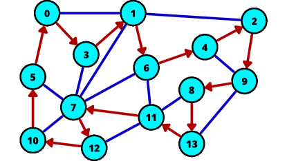
Figure 1: TSP graph with the solution $\vec{x}=(0,3,1,6,4,2,9,8,13,11,7,12,10,5)$. The blue edges represent possible paths that were not taken, and arrowed red edges represent the path taken by the solution. Edges with weight considered infinite are not represented.

With this formulation, the problem can be expressed as

$$\vec{x}_{opt}=\arg\min_{\vec{x}}\left(C\left(\vec{x}\right)\right)$$

$$x_{t}\in[0,N-1]\ \forall t\in[0,N-1]$$

$$x_{t}\neq x_{t^{\prime}}\qquad\forall t\neq t^{\prime}\in[0,N-1]$$

$$C(\vec{x})=\sum_{t=0}^{N-1}C_{x_{t},x_{t+1}},$$ (1)

where $C(\vec{x})$ is the cost function of the problem, $C_{i,j}$ is the cost of moving from node $i$ to node $j$ and $x_{N}=x_{0}$ is the starting -and final- node. If two nodes $i$ and $j$ are not meant to be connected, $C_{i,j}=\infty$. In the tensor that stores $C_{i,j}$ we include the information of whether it is a directed or undirected graph, which for our method will be indifferent in terms of complexity. In the non-symmetrical cost case, $C_{i,j}\neq C_{j,i}$.

The problem can be naturally extended for the $x_{0}\neq x_{N}$ just adjusting the summation limits.

The problem can also be generalized for the case that, at each step $t$, the costs of going from node $i$ to node $j$ change, we can generalize the cost function to

$$C(\vec{x})=\sum_{t=0}^{N-1}C_{t,x_{t},x_{t+1}},$$ (2)

where $C_{t,i,j}$ is the cost of moving from node $i$ to node $j$ at step $t$. If there is no returning condition, $C_{N-1,a,b}=0\ \forall a,b$.

We can also include an extra cost for arriving at a node at a each time step. This would represent, for the canonical interpretation of the TSP, the time spent by the salesman actually performing each sale at node $a$. This would be an extra linear term, so that the cost would be

$$C(\vec{x})=\sum_{t=0}^{N-1}\left(C^{0}_{t,x_{t}}+C_{t,x_{t},x_{t+1}}\right),$$ (3)

with $C^{0}_{t,i}$ as the cost of being at node $i$ at step $t$. If a node $a$ is fixed to be visited at time $t$, $C^{0}_{t,a}=-\infty$. If a node $a$ cannot be visited at time $t$, $C^{0}_{t,a}=\infty$.

Absorbing the linear term $C^{0}_{t,i}$ into all the relevant quadratic terms, $\hat{C}_{t,i,j}$, the cost function will be

$$C(\vec{x})=\sum_{t=0}^{N-1}\hat{C}_{t,x_{t},x_{t+1}}.$$ (4)

We can see that this problem can be expressed as a Quadratic Unconstrained Discrete Optimization (QUDO) problem with nearest neighbor interactions in a one-dimensional chain with the additional constraint of non-repetition.

3 Tensor Network solver

Our method will evaluate a uniform superposition of $\hat{N}$ variables, one for each timestep, in a qudit formalism, that can each be in $\hat{N}$ different basic states, one for each node $i$. The number $\hat{N}$ will vary according to the instance we are solving. On this superposition we will apply an imaginary time evolution that will cause the amplitudes of the base states $\vec{x}$ to decrease exponentially with the cost $C(\vec{x})$ of the combination. After that, we will apply a set of projectors to stay in the subspace that meets the constraints and finally determine the remaining state of maximum amplitude with an iterative partial trace.

Our algorithm is based on the method presented in [6], designed for unconstrained single-neighbor QUDO problems, with the inclusion of new MPO (Matrix Product Operator) layers for the constraints.

For the formulation in eq. (1), since all nodes have to appear once and the cost does not depend on which is the first node of the route because of the returning condition, we can fix one of them. We will fix $x_{N-1}=N-1$, that is: we will make sure the ‘$N-1$’th node we visit is the node with $i=N-1$. Therefore, we will only need to solve for the other $\hat{N}=N-1$ steps of the route. If we did not have the returning condition, we could just solve the problem as it is, with $\hat{N}=N$.

In general, if we want to make a route between two fixed points, we will only have to fix $x_{0}$ and $x_{N-1}$ and perform the algorithm on the other $\hat{N}=N-2$.

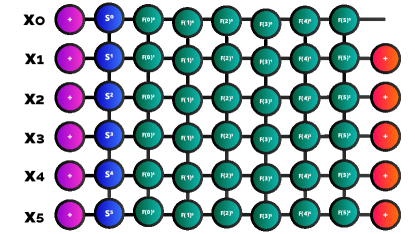
Figure 2: TSP tensor network.

Once we have the QUDO problem to solve and build its tensor network, we have to add the constraints with the inclusion of new MPO layers. Fig. 2 shows the tensor network that will be built, where the tensor layers ‘+’ and ‘$S$’ are the ones introduced by the method [6], with the ‘$F$’ layers that will enforce the constraints.

We have the + tensors that implement the uniform superposition of all possible combinations as our qudits, the $S$ tensor layer implements the imaginary time evolution using the $\hat{C}_{i,x_{i},x_{i+1}}$ tensor of our problem, and each $F(a)$ tensor layer that ensures that node $a$ only appears once in the combination. For any tensor $T^{i}$, the superscript $i$ indicates that the tensor is connected on the line of qudit $i$.

Using the notation presented in Fig. 3, these tensors $F(a)^{0}$ (Fig. 3 a) and $F(a)^{\hat{N}-1}$ (Fig. 3 c) will have indexes $i,j$ of dimension $\hat{N}$ and index $k$ of dimension $2$, while the $F(a)^{n}$ (Fig. 3 b) in the rest of the cases, their indexes $i,j$ will still have dimension $\hat{N}$, while the indexes $k,l$ will have dimension $2$. These bond indexes will have the function of communicating whether a certain node $a$ of the TSP graph has appeared up to that point or not. Its non-zero elements will be those in which $i=j$ and

$$F(a)^{0}_{ijk}=1\begin{cases}i,k=a,1\\ i,k=b,0\end{cases}$$ (5)

$$F(a)^{n}_{ijkl}=1\begin{cases}i,k,l=a,0,1\\ i,k,l=b,0,0\\ i,k,l=b,1,1\\ \end{cases}$$ (6)

$$F(a)^{\hat{N}-1}_{ijk}=1\begin{cases}i,k=a,0\\ i,k=b,0\\ i,k=b,1\\ \end{cases}$$ (7)

for $\forall b\neq a\in[0,\hat{N}-1]$ pairs of different nodes.

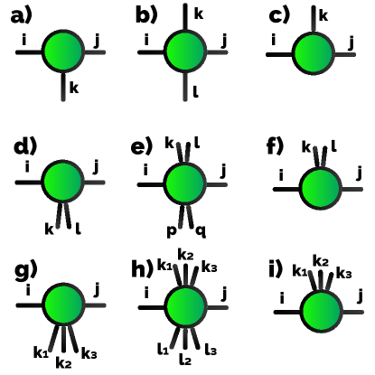
Figure 3: Notation for all indexes used in all tensors in this paper. a), b), c) Tensors with 1 bond index, d), e), f) Tensors with 2 bond index, g), h), i) Tensors with 3 bond index.

We apply the iterative method of resolution, choosing randomly when encountering cases with degenerate cost, and we obtain the different steps of the path. After each step, because the chosen node cannot be chosen again, in the ‘+’ tensors we remove the states of this chosen nodes, as well as remove their filter layers.

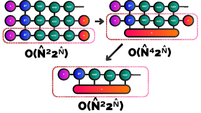
Figure 4: Contraction scheme for 3 variables with the cost of its steps for $\hat{N}$ variables.

Our contraction scheme will be the presented in Fig. 4. Contracting the layers for each qudit of the tensor network with $\mathcal{N}$ variables requires $O(\mathcal{N}^{4}2^{\mathcal{N}})$ steps, and having to contract $O(\mathcal{N})$ layers, we have that the complexity for determine one variable is $O(\mathcal{N}^{5}2^{\mathcal{N}})$ with a memory cost of $O(\mathcal{N}^{2}2^{\mathcal{N}})$. Using the fact that each variable is less expensive than the previous one to compute, because of the iterative reduction of layers and nodes, we have that the complexity to solve an integer TSP of $\hat{N}$ variables is $O(\hat{N}^{5}2^{\hat{N}})$ with a memory cost of $O(\hat{N}^{2}2^{\hat{N}})$. We emphasize the fact that the tensors involved are highly sparse.

We see that this method is better than doing a blind brute-force search, which would require $O(N!)$ operations.

4 Generalized TSP cases

4.1 Different number of steps than number of nodes

We can generalize the problem to other cases of industrial interest. The first case is the case where we have $N^{s}$ time steps, $N$ nodes and each node $i$ can be visited between $N^{0}_{i}$ and $N^{f}_{i}$ times.

In this case, we will make a tensor network with the same structure as before, with $N^{s}$ qudits, but with a change in the filter layers. We will now generalize the tensors $F(a)$, which used to make sure that each node has appeared exactly once in our solution, as tensors $F(a,N^{0}_{a},N^{f}_{a})$, which will make sure that node $a$ only appears between $N^{0}_{a}$ and $N^{f}_{a}$ times.

The tensors $F(a,N^{0}_{a},N^{f}_{a})^{0}$ (Fig. 3 d) and $F(a,N^{0}_{a},N^{f}_{a})^{N^{s}-1}$ (Fig. 3 f) will have indexes $i,j$ of dimension $N$ and index $k$ of dimension $N^{f}_{a}+1$, while the $F(a,N^{0}_{a},N^{f}_{a})^{n}$ (Fig. 3 e) in the rest of the cases, their indexes $i,j$ will have dimension $N$, while the indexes $k,l$ will have dimension $N^{f}_{a}+1$. These bond indexes will have the function of communicating how many times a certain node $a$ of the TSP graph has appeared up to that point. The bond indexes can have a smaller dimension, adapting to the step in which we are. However, we will not consider this adaptation in the paper, as it would only complicate the analysis. Its non-zero elements will be those in which $i=j$ and

$$F(a,N^{0}_{a},N^{f}_{a})^{0}_{ijk}=1\begin{cases}i,k=a,1\\ i,k=b,0\end{cases}$$ (8)

$$F(a,N^{0}_{a},N^{f}_{a})^{n}_{ijkl}=1\begin{cases}k<N^{f}_{a},\ i,l=a,k+1\\ i=b,\ k=l\\ \end{cases}$$ (9)

$$F(a,N^{0}_{a},N^{f}_{a})^{N^{s}-1}_{ijk}=1\begin{cases}N^{0}_{a}<k+1<N^{f}_{a},&i=a\\ N^{0}_{a}<k<N^{f}_{a},&i=b\\ \end{cases}$$ (10)

for $\forall b\neq a\in[0,N-1]$.

As before, we will use the iterative method to obtain the different nodes in the different time steps. Here, after determining in one step $i$ the node $a$, in the next iteration we will reduce $N^{0}_{a}$ and $N^{f}_{a}$ by one unit. If $N^{0}_{a}$ reaches 0, it stops decreasing. If $N^{f}_{a}$ reaches 0, we remove the filter layer from that node and eliminate that possibility in the ‘+’ tensors. In case $N^{f}_{a}>N-1$ and $N^{0}_{a}=0$ at some step, that filter layer can be removed, since the node loses the appearance constraint.

To analyze the computational complexity, without loss of generality let us assume that each node can appear up to a uniform number of $N^{f}$ times. The complexity of collapsing the layers for a qudit would be $O(N^{4}(N^{f})^{N})$. By contracting the $N^{s}$ layers and repeating for the $N^{s}$ variables to be determined, we would have a complexity of $O(N^{4}(N^{s})^{2}(N^{f})^{N})$ with a memory cost of $O(N^{2}(N^{f})^{N})$.

4.2 Non-markovian TSP

The second case we will study is the TSP with memory. This problem consists of a generalization in which the cost of a step depends not only on the previous step, but also on the previous ones up to a certain term. In this case we stop having a QUDO case and we move to a HODO (Higher Order Discrete Optimization) case.

For a number of steps $K$ to be considered in each time slot, we will have the cost function

$$C(\vec{x})=\sum_{t=0}^{N-1}C_{t,x_{t+1},x_{t},x_{t-1},\dots,x_{t-K+1}},$$ (11)

being $C_{t,i,j_{0},\dots,j_{K-1}}$ the cost of moving from node $j_{0}$ to node $i$ at step $t$ with $j_{1},\dots,j_{K-1}$ being the last $K$ nodes. If $t<K$, we only use the nodes until $x_{0}$ or $x_{N-n}=x_{-n}$ if we want the returning condition.

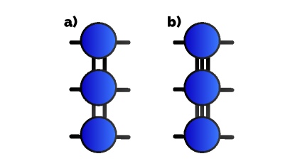
Figure 5: MPO layer for 3 multiple bond index tensors.

For this problem, we will change the tensor layer $S$ to a tensor MPO layer $S(K)$ where for each bond index $k,l$ we will put $K$ bond indexes $k_{m},l_{m}$, as in Fig. 3. Each of them will pass the signal from a previous node and an imaginary time evolution will be applied according to the signal obtained through the input indexes. Thus, the non-zero elements of these tensors will be those with $i=j=l_{0}$ and $l_{m+1}=k_{m}\ \forall m\in[0,K-2]$. They will be connected as Fig. 5.

The value of its elements will be analogous to that described in general terms in [6]. The rest of the method is analogous to that used in the previous cases, and can be combined with the generalization of Ssec. 4.1, since in it only the filtering layers are changed and in this one only the evolution layer.

Its computational complexity will be $O(N^{2K+2}2^{N})\ \forall K>1$ with memory cost $O(N^{2K+1}2^{N})$ in the simple case and $O(N^{2K+2}(N^{s})^{2}(N^{f})^{N})$ with memory cost $O(N^{K+1}(N^{f})^{N})$ in the version of Ssec. 4.1.

4.3 Bottleneck TSP

The variant we are going to solve now is the TSP with bottleneck. The problem is to find the route which minimizes the cost of the highest-cost edge of the route. The applications of this problem are multiple, such as bus route planning or the design of plate drilling routes.

The formulation of this problem is

$$\vec{x}_{opt}=\arg\min_{\vec{x}}\left(\max\left(C_{x_{t},x_{t+1}}\right)\right)$$ (12)

$$x_{t}\in[0,N-1]\ \forall t\in[0,N-1]$$

$$x_{t}\neq x_{t^{\prime}}\qquad\forall t\neq t^{\prime}\in[0,N-1],$$

To solve this problem, we will use the same scheme as in Fig. 2, but changing the $S$ tensor layer to a $Z$ tensor layer. Now this layer will be in charge of communicating which is the highest displacement cost. It final tensor will be responsible for applying the imaginary time evolution. For the same reason, we will need that instead of having a single index bond that communicates the node of the previous step, we will have two that communicate the previous node and the maximum cost that has appeared until that step.

For this method we will assume that all elements of the tensor $C$ are positive integers. The generalization to rational numbers and the approximation to integers with truncation is straightforward. For the sake of simplicity, we also assume the returning condition, generalization to other cases is straightforward.

Its physical indexes $i,j$ are of dimension $N-1$ and its bond indexes $k,l$ for the node signal in the previous step are of dimension $N-1$ and its bond indexes $q,p$ for carrying the maximum cost signal are of dimension $\max\left(C_{a,b}\right)\ \forall a,b$. The non-zero elements of these tensors will be those in which $i=j=k$ for the $Z^{0}$, $i=j=l$ for the $Z^{n}$ and $i=j$ for the $Z^{N-2}$. These non-zero elements will be

$$Z^{0}_{ijkq}=1\text{ if }q=C_{x_{N-1},i}$$ (13)

$$Z^{n}_{ijklqp}=1\text{ if }p=\max(q,C_{k,i})$$ (14)

$$Z^{N-2}_{ijkq}=e^{-\tau\max(q,C_{k,i},C_{i,x_{N-1}})}$$ (15)

for $\forall b\neq a\in[0,N-2]$, being $\tau$ the decay hyperparameter.

Another variation would be to find the path that maximizes the cost of the lowest-cost edge of the path. This variant is useful for the scheduling of metalworking steps in aircraft manufacture, where we need to avoid accumulating heat in steps close together in space and time.

The rest of the algorithm is exactly the same as the previous ones, but changing the $Z^{0}$ so that its non-zero elements are at $q=\max(C_{x_{m-1},x_{m}},C^{\max}_{m})$, being $m$ the variable we want in this step and $C^{\max}_{m}$ the highest cost found up to this step.

To solve this version, we only have to do the same as in the minimization version, but changing all the $\max$ by $\min$ and vice versa and using a $\tau<0$ for maximizing.

4.4 Politician TSP

Another variant with industrial utility is the traveling politician problem, which deals with states that have several cities each and you have to visit exactly one city in each state. This can be abstracted as a graph with $N$ nodes of different $M$ classes so that we have to visit one node of each class. Its industrial utility includes the more optimal cutting of types of sheets of paper from a larger sheet.

The formulation of this problem is

$$\vec{x}_{opt}=\arg\min_{\vec{x}}\left(C\left(\vec{x}\right)\right)$$

$$x_{t}\in[0,N-1]\ \forall t\in[0,N-1]$$

$$x_{t}\neq x_{t^{\prime}}\qquad\forall t\neq t^{\prime}\in[0,N-1]$$

$$\text{if }x_{t}\in G_{k}\rightarrow x_{t}^{\prime}\notin G_{k}\ \forall t\neq t^{\prime}\in[0,N-1]$$

$$C(\vec{x})=\sum_{t=0}^{N-1}C_{t,x_{t},x_{t+1}},$$ (16)

being $G_{k}$ the $k$-th class.

To solve this problem, we will change the filter layers $F$ in a very simple way. We will make that, instead of the layer being associated to the node, it will be associated to the group. That is, instead of activating signal 1 and filtering only for an incoming state, now the tensors will activate signal 1 and filter for all the states of the corresponding group.

The rest of the algorithm is exactly the same, except that each time a node of a class appears, we remove the initialization and the filtering layer not only of that node, but of all nodes of its same class.

Its complexity will be $O(N^{5}2^{M})$ with a memory cost of $O(N^{2}2^{M})$.

4.5 TSP with precedence

Another interesting case is the TSP in which we have a precedence rule between nodes. That is, certain nodes have to appear earlier in the route than others. This additional rule is straightforward to implement in the first version of the algorithm by slightly modifying the tensors $F(a)$. We will see how to do it with an example.

Let us imagine that we have the rule that node 4 has to appear before node 7 in the path. To take this into account, we will only have to make the tensors of layer $F(4)$, in case a 0 arrives for index $k$, let all the states pass through $i$ except for $i=7$. Also, node $7$ cannot appear first and $4$ cannot appear last, which is embodied in the initialization. The rest of the algorithm is exactly the same.

5 Proof of Concept for the ONCE

We will now present a real use case in which we have applied this method [7]. This is the case of the Job Reassignment Problem (JRP) developed for Organización Nacional de Ciegos Españoles (ONCE).

5.1 Problem description

The Job Reassignment Problem consists of, given a set of workers assigned each to one of a set of jobs, and a set of vacant jobs, finding whether any of the assigned workers should move to the vacant jobs. Each job will have its own quality score, given by its profitability, and an affinity with each of the workers, given by the suitability of this worker occupying that job. The objective is to obtain an outplacement that increases the sum of productivity and affinity in the group of workers.

Since the whole process is extensively analyzed in the original paper, we will focus on the subproblem, where given a set of workers and vacant positions, we have to choose which position to send them to (if any). The constraint will be that no two workers can be sent to the same job. Each worker can only be assigned to one job, but that will be assured by the encoding of the variables and will not be a restriction we need to impose to our tensor network.

The solutions will be encoded as a vector $\vec{x}$ of integer values, where $x_{i}$ will be the vacant position to which the worker $i$ is sent. Moreover, $x_{i}=0$ means that worker $i$ stays in his position without moving to any of the vacant ones. Its cost function will be

$$C(\vec{x})=\sum_{i=0}^{N-1}\left[c^{P}(P^{C}_{i}-P^{V}_{x_{i}})+c^{A}(A^{C}_{i,i}-A^{V}_{x_{i},i})\right],$$ (17)

being $P^{V}_{x_{i}}$ the quality of the $x_{i}$ vacant job, $P^{C}_{i}$ the quality of the current $i$ worker job, $A^{V}_{x_{i},i}$ the affinity of the worker $i$ at $x_{i}$ vacant job, $A^{C}_{i,i}$ the affinity of the worker $i$ at its current job, and $c^{V}$ and $c^{A}$ are proportion factors.

Therefore, we can see that our problem can be expressed as a general TSP problem as in eq. (3) in which we have only the $C^{0}$ term.

By the fact that we only have the linear term, we do not need the $S$ tensor layer, we can put the imaginary time evolution in the ‘+’ tensor of each variable itself. In addition, since several workers may not move jobs, we also remove the filter layer of $x_{i}=0$. The other filter layers will have $N^{0}=0$ and $N^{f}=1$, since a vacancy may not be chosen. After each choice step of $x_{i}$, if we obtain that $x_{i}\neq 0$, we remove that state from the ‘+’ tensors and its corresponding filter layer. If at any step we run out of free vacancies, we stop the algorithm and fill the remaining components of $\vec{x}$ with 0.

The computational complexity of solving a subproblem for $I$ vacant jobs and $J$ workers is $O(J^{2}I^{3}2^{I+1})$ with a memory cost of $O(I\ 2^{I+1})$.

Due to the symmetry of the problem, since assigning workers to jobs and jobs to workers is equivalent, in the case that $I>J$, we will only have to run the same algorithm with the cost tensor $C_{i,x_{i}}$ changed so that now the elements $x_{i}$ are the worker we send to vacant $i$ and $x_{i}=0$ means that no worker is sent to this vacant. Thus, the computational complexity will be $O(I^{2}J^{3}2^{J+1})$ with a memory cost of $O(J\ 2^{J+1})$.

5.2 Results

For the productive resolution of the JRP we compared three different methods: Dwave’s Advantage$\_$system4.1 Quantum Annealer, Azure’s Digital Annealer (DA) and the Tensor Networks method explained in this paper.

Initial comparisons showed good results for the three platforms, but Advantage$\_$system4.1 was discarded for lack of production-scale access.

For the comparison between DA and TN methods we selected 72 days at random from a whole year, in order to minimize the variations caused by seasonal effects. The day selection was also equiprobably selected amongst the seven days of the week.

The first thing we did in order to compare the two methods was to sum the total $\Delta P\equiv\sum_{i}P^{C}_{i}-P^{V}_{x_{i}}$ job quality gain of all days, that is, the accumulated difference between the qualities of the originally assigned jobs and the qualities of the reassigned jobs that each method suggested. It turned out that, for each of the 72 days, $\Delta P_{DA}=\Delta P_{TN}$. Then, as the problem itself minimizes the total cost function $C$ and not only $\Delta P$, we compared the other part of the cost function, $\Delta A\equiv\sum_{i}A^{C}_{i,i}-A^{V}_{x_{i},i}$, to break the tie. It did not. However, the solutions were not equivalent due to the existence of degeneration. For example, we found a case where the only available worker $i$, which was assigned to a low-quality job, could be reassigned to two different workplaces with the same high quality $P^{V}_{x_{i}}$. The worker also had the same $A^{V}_{x_{i},i}$ affinity with the two vacant workplaces. Then, the gain of choosing one or the other was identical, and the two methods -DA and TN- chose at random different non-equivalent answers.

The fact that the two methods agree to such extent, reaching the same accumulated cost throughout all days and only being distinguishable by differences in degenerate cases, give us strong confidence on both methods.

6 Conclusions

We have studied a new family of conceptually simple algorithms to deal with a set of different versions of the Traveling Salesman Problem using tensor networks and have shown their effectiveness in a real industrial case. Future lines of research could include the application of these algorithms to different TSP problems or to certain particular cases, the study of how to take advantage of the sparse characteristics of the tensors being used or the contraction of them with quantum resources, or even applying the techniques to problems outside the generalised TSP family of problems we discuss in this paper.

References

-
[1]
Adewole Philip, Akinwale Adio Taofiki and Otunbanowo Kehinde.
A Genetic Algorithm for Solving Travelling Salesman Problem,
International Journal of Advanced Computer Science and Applications(IJACSA), 2(1), 2011. -
[2]
Karthik Srinivasan, Saipriya Satyajit, Bikash K. Behera, Prasanta K. Panigrahi.
Efficient quantum algorithm for solving travelling salesman problem: An IBM quantum experience.
arXiv:1805.10928 [quant-ph], (2018). -
[3]
Edward Farhi, Jeffrey Goldstone, Sam Gutmann.
A Quantum Approximate Optimization Algorithm.
arXiv:1411.4028 [quant-ph], (2014). - [4] Peruzzo, A., McClean, J., Shadbolt, P. et al. Nat Commun 5, 4213 (2014).https://doi.org/10.1038/ncomms5213
-
[5]
Jacob Biamonte, Ville Bergholm.
Tensor Networks in a Nutshell.
arXiv:1708.00006 [quant-ph], (2017). -
[6]
Alejandro Mata Ali, Iñigo Perez Delgado, Marina Ristol Roura, Aitor Moreno Fdez. de Leceta.
A Quantum-Polynomial-time Solver of Tridiagonal QUBO and QUDO problems with Tensor Networks.
arXiv:2309.10509 [quant-ph], (2023). -
[7]
Iñigo Perez Delgado, Beatriz García Markaida, Alejandro Mata Ali, Aitor Moreno Fdez. de Leceta.
QUBO Resolution of the Job Reassignment Problem.
arXiv:2309.16473 [quant-ph], (2023).