An Adaptive Fast-Multipole-Accelerated Hybrid Boundary Integral Equation Method for Accurate Diffusion Curves

Abstract.

In theory, diffusion curves promise complex color gradations for infinite-resolution vector graphics. In practice, existing realizations suffer from poor scaling, discretization artifacts, or insufficient support for rich boundary conditions. Previous applications of the boundary element method to diffusion curves have relied on polygonal approximations, which either forfeit the high-order smoothness of Bézier curves, or, when the polygonal approximation is extremely detailed, result in large and costly systems of equations that must be solved. In this paper, we utilize the boundary integral equation method to accurately and efficiently solve the underlying partial differential equation. Given a desired resolution and viewport, we then interpolate this solution and use the boundary element method to render it. We couple this hybrid approach with the fast multipole method on a non-uniform quadtree for efficient computation. Furthermore, we introduce an adaptive strategy to enable truly scalable infinite-resolution diffusion curves.

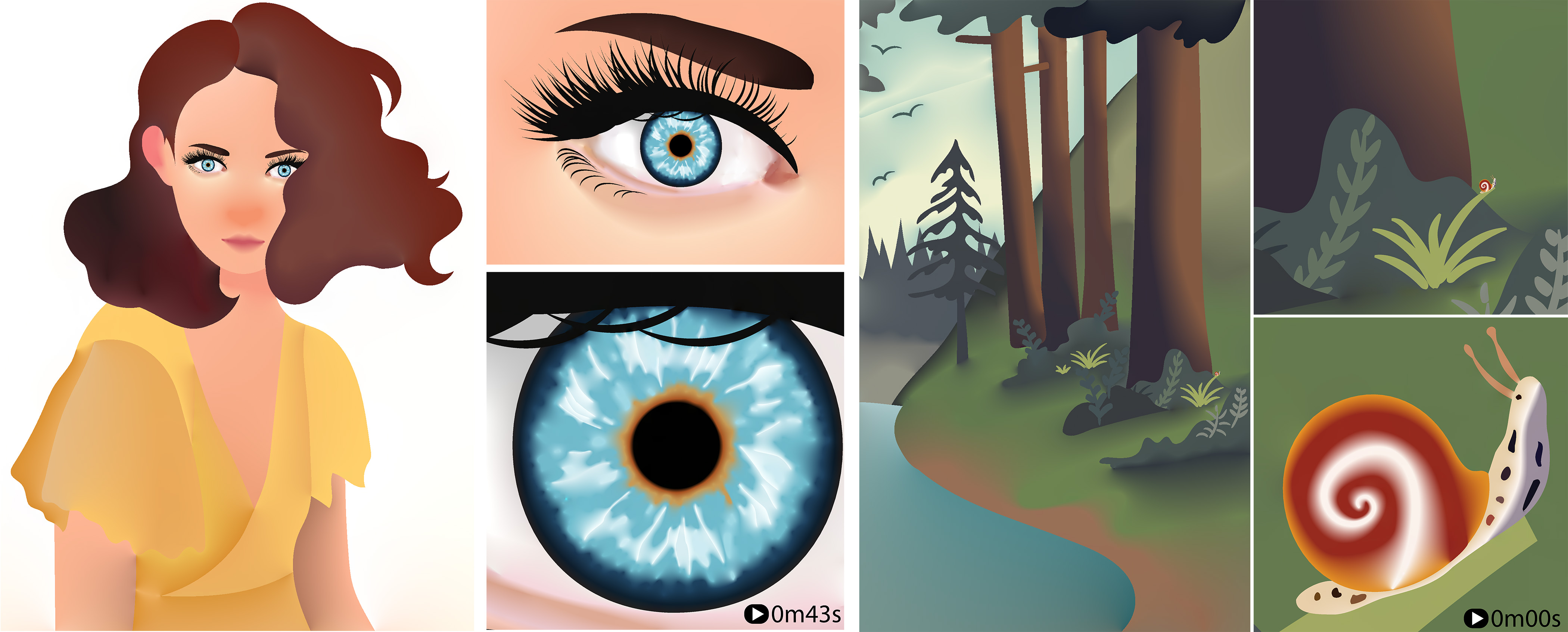
Figure 1. A diffusion curve image drawn with our method demonstrates that extremely zoomed-in views maintain high accuracy. Please enjoy these images best using a high-resolution digital screen (or by printing on billboard). See the accompanying demo video for full-frame zoom-in transition on a given timestamp. We obtained the vector graphics image from buysellgraphic.com with purchased commercial license and have modified it to enable extreme zoom-in.

1. Introduction

Diffusion curves are primitives for smoothly interpolating color data in vector graphics images, where the continuous color data is defined to be the solution to Laplace’s equation with boundary values specified along vector graphics curves. Laplace’s equation is the prototypical elliptic partial differential equation (PDE), and at first glance it would appear that any numerical method for elliptic PDEs could potentially be used to solve it, such as finite differences, finite elements, boundary elements or random walks. Unfortunately, in practice, diffusion curves present a number of complications which cause problems in many existing numerical methods.

Finite difference-based diffusion curve methods (Orzan et al., 2008; Finch et al., 2011) rely on lossy rasterization of boundary data onto a fixed pixel grid, which may either be too dense (and slow) or too coarse (and inaccurate and aliased) for a desired display resolution. Finite element methods (Pang et al., 2011; Jacobson et al., 2012) similarly commit to a fixed, albeit adaptive, grid resolution which simultaneously determines the solution accuracy, solution smoothness, and boundary curve fidelity. Both linear elements and isogeometric (curved) elements present their own respective difficulties. While popular, linear FEM requires approximating curved Bézier curves by linear segments. Alternatively, higher-order FEM, with its more complicated functions spaces (Schneider et al., 2018; Ilbery et al., 2013) could be used on a mesh made of curved elements which conform to boundary curves. Unfortunately, generating these meshes automatically remains an open problem with very recent advances (Hu et al., 2019; Mandad and Campen, 2020). Furthermore, once meshes are generated, FEM struggles to provide accuracy near boundary singularities (Gopal and Trefethen, 2019a). Unlike many other PDE-based problems in computer graphics, diffusion curves are rife with both geometric boundary singularities (sharp corners or endpoints of open curves) and discontinuities in prescribed color values. Stochastic methods based on random walks, like the recent Walk on Spheres method (Sawhney and Crane, 2020), can overcome some of these difficulties, however, such methods do not support problems where the boundary conditions are predominantly Neumann, which are essential to practical applications of diffusion curves.

An alternative to discretizing the entire image domain is to employ boundary-only methods, where the color value at every point can be computed from calculations performed on the boundary alone. The boundary element method (BEM) discretizes only the boundary using boundary elements, and can then evaluate the solution at any point in the domain after a precomputation step which involves solving an integral equation. BEM, however, still requires discretization of the boundary into line segments (van de Gronde, 2010; Sun et al., 2012), which can lead to resolution problems at the boundary, similar to those encountered in linear FEM.

We propose a boundary-only method which does not represent the solution on line segments approximating the boundary geometry. Instead, we sample directly from the exact spline representation of boundary curves using the boundary integral equation method (BIEM), and solve the associated integral equation in a way that allows us to color pixels at an arbitrary resolution. To evaluate the color data, we interpolate our smooth BIEM solution to a resolution- and viewport-aware BEM discretization. A large part of the calculations required by our method can be precomputed and, during changes of the viewport, the solution to the BIE only needs to be re-solved on a sparse set of boundary curves. We employ the Fast Multipole Method (FMM) to efficiently evaluate the color data for a large number of curves. In applying the FMM to diffusion curves, we find that the FMM, as it is typically presented (Martinsson, 2019) and implemented (Greengard and Gimbutas, 2022), is not especially friendly to a graphics audience, and forgoes some precomputations which we find to be essential in our application. Thus, we provide a self-contained presentation of the FMM in the context of diffusion curves, along with the novel strategies we employ to accelerate our computations. Our method, together with our optimized FMM, results in an efficient and fully adaptive infinite-resolution algorithm for evaluating diffusion curves, and can be viewed as a hybrid of BEM and BIEM, which maximally exploits the advantages of both.

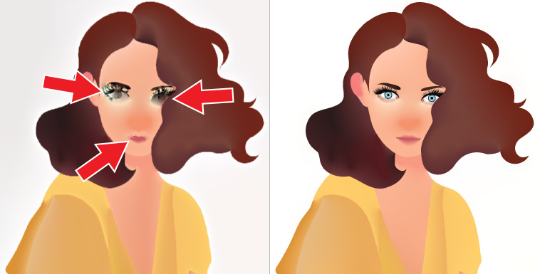
Figure 2. The original finite-difference method of Orzan et al. (2008) exhibits inaccuracies (left), e.g., around the eye. Our hybrid, boundary-only method shows accurate solution (right).

2. Related Works

2.1. Diffusion Curves

When Diffusion Curves (DCs) were first introduced, Orzan et al. (2008) solved Laplace’s equation using the Finite Difference (FD) Method, with follow-up work reformulating the equation as a constraint problem (Bezerra et al., 2010) on a grid of pixels. Despite its strengths of simplicity and easy parallelization, rasterizing the input curve to a pixel domain can lead to inaccurate results, as shown in Fig. 2 (left). Follow-up work of (Jeschke et al., 2009) overcomes this issue by initializing each pixel to the color of the closest curve point and blending the image with a Jacobi-like iteration. While resulting images are visually excellent, they can nonetheless differ slightly from the converged solutions.

To overcome some of the problems of the FD method, the Finite Element Method (FEM) was employed to evaluate DCs (Pang et al., 2011; Takayama et al., 2010) since FEM can more precisely represent the boundary geometry using constrained triangulation along curves. While the boundary can indeed be better represented, triangulation itself can become burden if the input curves are too numerous or have complex shapes. Using the powerful triangulation tool TriWild (Hu et al., 2019), we could not successfully generate a triangulation of example Fig. 2 with sufficient detail preserved. Even if triangulation succeeds, FEM still suffers from bleeding artifacts if the triangulation is not dense enough, as shown in Fig. 3. FEM has notoriously poor accuracy near singularities such as re-entrant corners, which are commonplace in DCs (see, e.g., (Gopal and Trefethen, 2019a)). While (Boyé et al., 2012) (Sec.4.3) did present a heuristic method to circumvent this singularity problem, it does not provide as accurate a solution as our approach does.

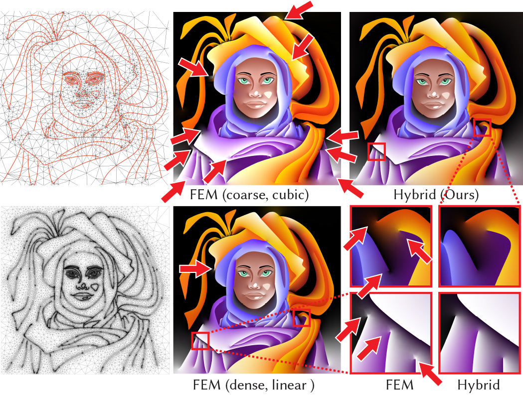
Figure 3. Top row: Bleeding artifacts are pervasive in the FEM results of TriWild (Hu et al., 2019), as shown in their Figure 12, reproduced here with arrows added. (Used under permission.) Bottom row: With much denser triangulation, with linear elements, it still shows unnatural transition of color near end point of curves. Our method shows accurate and smooth solution with the same data.

The Boundary Element Method (BEM) (van de Gronde, 2010; Sun et al., 2012) can be used to avoid triangulation by only discretizing boundary curves and re-formulating the problem as an integral equation. The evaluation of color values, which would otherwise be fairly expensive with brute force computation, can be accelerated using the Fast Multipole Method (FMM) (Sun et al., 2014). However, BEM still suffers from visible polyline discretization, as shown in Fig. 4 (b).

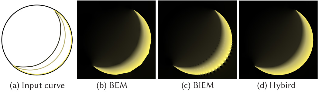
Figure 4. Result comparisons between BEM, BIEM, and our Hybrid method. BEM suffers from visible polyline, and BIEM shows dotted-looking artifacts near the boundary, whereas our method is free from both problems.

Diffusion curves can also be evaluated using stochastic methods. Stochastic ray tracing (Bowers et al., 2011) treats the curves as light sources emitting radiant energy, and determines the color at a pixel by computing the radiance received at that point. This method was further combined with FEM in follow-up work (Prévost et al., 2015). While stochastic ray tracing is able to achieve real-time performance using a GPU-based implementation, it is unable to diffuse colors around corners or obstacles, resulting in visual differences when compared with diffusion curves evaluated by other methods. The fully meshless Walk on Spheres (WoS) (Sawhney and Crane, 2020; Sawhney et al., 2022), on the other hand, does diffuse colors around obstacles. However, WoS has difficulties with Neumann boundary conditions, and this turns out to be a major limitation, since such boundary conditions turn out to be exceedingly useful in practice. For complicated collections of input curves, it is difficult to specify Dirichlet boundary conditions on every single curve. By specifying a zero Neumann boundary condition on a majority of the input curves, one only needs to specify Dirichlet boundary conditions on a small subset of curves to create a smooth and natural color interpolation on the domain, as shown in Fig. 5.

Besides the various methods for evaluating diffusion curves, the notion of a diffusion curve itself has been generalized in several directions. The typical definition of the interpolated colors of a diffusion curve is as a harmonic function; this definition has been generalized to a biharmonic function with FD (Finch et al., 2011), FEM (Boyé et al., 2012; Jacobson et al., 2012), and BEM (Ilbery et al., 2013). A blending of two harmonic functions (Jeschke, 2016) has also been introduced to overcome some of the unintuitive extrapolation behaviour of biharmonic functions. Diffusion curves with harmonic interpolated colors satisfying Laplace’s equation have been generalized to interpolated colors satisfying Poisson’s equation (Hou et al., 2020), where the inhomogeneous term in the Poisson equation was used to provide more nuanced control over blending and diffusion. Finally, while diffusion curves are typically presented as an artistic tool, methods have been proposed for constructing diffusion curve images from rasterized images (Jeschke et al., 2011; Xie et al., 2014; Zhao et al., 2017).

Furthermore, it’s important to note that, besides diffusion curves, there exists a multitude of other approaches to color gradations in vector graphics representations. One such example is the patch-based method (Xia et al., 2009). However, we will not cover other approaches in this paper.

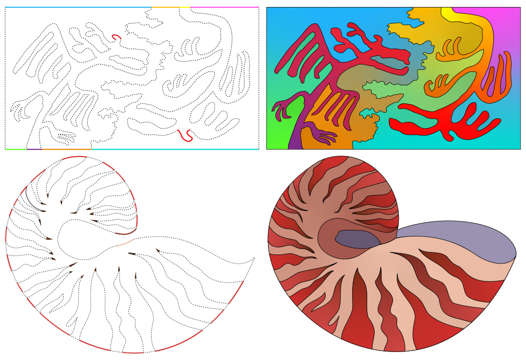
Figure 5. Input diffusion curves, with Dirichlet boundary conditions on colored curves and zero Neumann boundary conditions on dotted curves (left), and its solution (right), with an example image inspired from (Hofstadter, 1979) (top) and an example of a Nautilus shell (bottom). For the Nautilus shell example, a solid color inner shell region is overlayed. Nautilus shell vector graphics art is obtained from buysellgraphic.com with purchased commercial license.

2.2. BEM & BIEM in Graphics

The Boundary Element Method (BEM) reformulates the PDE to be solved as a boundary integral equation. It then discretizes this integral equation by approximating the boundary curves by line segments in 2D, or by approximating the boundary surfaces by triangular elements in 3D. It then represents the solution to the integral equation as a piecewise constant function on these line segments or flat surface elements. BEM was first introduced in the graphics community for real time deformable objects (James and Pai, 1999), followed by ocean wave animation (Keeler and Bridson, 2014; Schreck et al., 2019), and surface only liquids simulation (Da et al., 2016). BEM can accelerate simulations while retaining visual accuracy, in those cases where the simulation involves only the boundary of the object in question.

The Boundary Integral Equation Method (BIEM) (Greengard et al., 2009) uses the same integral equation formulations employed by the BEM, with the difference being that the BIEM represents the curve and the data by spectrally-accurate quadrature-based discretizations, where by spectrally-accurate, we mean discretizations for which the approximation error decays exponentially with the number of degrees of freedom used. This efficient representation means that a very small number of degrees of freedom are required to represent the solution to high accuracy. As far as we know, there is no work that employs BIEM in the graphics community. The BIEM has gained popularity for simulations in mathematical physics due to its simple quadrature-based integration scheme, its favorable conditioning properties, and its high accuracy. Although evaluating the solutions of BIEM close to boundaries presents substantial challenges (Helsing and Ojala, 2008), it happens that, in many physics-related applications, e.g., acoustic scattering, the solution is mainly desired away from the boundaries.

2.3. FMM in Graphics

The Fast Multipole Method (FMM) (Greengard and Rokhlin, 1987) has been sporadically explored in the computer graphics community. Sun et al. (2014) introduced the FMM for diffusion curves with a simple uniform quadtree structure. The FMM has also been used for fast computations of repulsive curves (Yu et al., 2021), ferrofluids (Huang et al., 2019), and fast linking numbers (Qu and James, 2021). Fast summation methods similar to FMM have been employed in graphics, e.g., to compute winding numbers (Barill et al., 2018) and to simulate fluids (Zhang and Bridson, 2014).

3. Overview of Methods

We begin by formulating a boundary value problem using different discretization approaches: the Boundary Element Method (BEM), the Boundary Integral Equation Method (BIEM), and our Hybrid Method, which combines the strengths of BEM and BIEM. We include Neumann boundary conditions in our framework for the diffusion curve problem.

While our proposed Hybrid Method offers notably improved accuracy compared to BEM, BIEM, and previous methods, its computational efficiency is suboptimal if applied naively to a complex diffusion curve image. To address this, we incorporate the Fast Multipole Method (FMM) for faster computations. The efficiency of the FMM is enhanced by incorporating a non-uniform quadtree approach, departing from the previously used uniform quadtree (Sun et al., 2014). This efficiency improvement is complemented by the precision gains achieved through quadtree clipping. The density values are obtained through the Generalized Minimum Residual (GMRES) algorithm.

To enable detailed zoom-in into localized parts of a diffusion curve image, we introduce an adaptive strategy that efficiently re-solves local density values without requiring a full re-solve of the entire image.

Finally, we present an anti-aliasing scheme involving weighted integration, leveraging the structure of the non-uniform quadtree.

Our main contributions can be summarized as follows:

• We perform a comprehensive comparison of BEM and BIEM, leading to the development of a hybrid method that effectively utilizes their respective strengths.

• We adopt the Neumann boundary condition for diffusion curve problems.

• We implement the FMM using a non-uniform quadtree approach, combined with quadtree clipping, resulting in rapid and accurate computation of diffusion curves.

• We introduce an adaptive strategy for optimal discretization tailored to the viewport.

• We introduce an anti-aliasing scheme based on the non-uniform quadtree structure.

4. Boundary Value Problem

Before considering the more complicated case of diffusion curves, where double-sided boundary conditions are specified over a collection of open curves, we consider the model problem of Laplace’s equation on region $V\subset\mathbb{R}^{2}$ with a simple, closed boundary $S$:

(1) $$\Delta u=0\;\textrm{on}\;V,\quad\text{ subject to one of }\quad\begin{cases}\text{$u=u^{*}$ on $S$},\\ \text{$\frac{\partial u}{\partial n}=\psi^{*}$ on $S$}.\end{cases}$$

For simplicity of presentation, we will only consider the Dirichlet boundary condition until Sec. 5.4.

We discuss three approaches to solving this problem: the boundary element method (BEM), the boundary integral equation method (BIEM), and our newly proposed hybrid of BEM and BIEM.

4.1. Boundary Integral Equation

Both the BEM and the BIEM reformulate the underlying PDE over the volume $V$ as boundary integral equations over the boundary $S$. The key idea is to use a representation involving the free-space Green’s function, which ensures that the candidate solution always satisfies the PDE. The problem is thus reduced to enforcing the correct boundary conditions on $S$.

4.1.1. Green’s function

The free space Green’s function $G$ is defined to be the solution to the Laplace equation

(2) $$\Delta G(p,q)=\delta(p,q),$$

where $p,q\in\mathbb{R}^{2}$. The Dirac delta function $\delta(p,q)$ represents a unit impulse at the source point $p$, and $G(p,q)$ represents the response at the point $q$ due to that source.

The Green’s function for Laplace’s equation in two-dimensional Euclidean space, as well as its directional derivative, are well known to be

(3) $$G(p,q)=-\frac{\log(\|p-q\|)}{2\pi}$$

and

(4) $$F(p,q)=\frac{\partial G(p,q)}{\partial n(p)}=-\frac{(p-q)\cdot n(p)}{2\pi\|p-q\|^{2}},$$

respectively. Where $n(p)$ is the normal vector at $p$.

4.1.2. Integral Equation

Using the free space Green’s function, we can convert the boundary value problem Eq. 1 into its Boundary Integral Equation (BIE) formulation. Consider the so-called single layer potential, which represents our candidate solution $u$ as an integral of the Green’s function over a boundary density $\sigma$:

(5) $$u(x)=\int_{S}G(p,x)\sigma(p)dS(p),\quad\forall x\in V.$$

Letting $x$ approach the boundary $S$, we obtain the following BIE, which we can solve for the unknown density $\sigma(p)$ on the boundary given Dirichlet boundary values $u^{*}(q)$:

(6) $$u^{*}(q)=\int_{S}G(p,q)\sigma(p)dS(p),\quad\forall q\in S.$$

The process of solving the boundary value problem Eq. 1 using its BIE formulation can be broken into two distinct stages. We call process of solving for the density $\sigma(p)$ using Eq. 6 the solution stage, and the process of evaluating our solution $u(x)$ on domain using formula Eq. 5 the evaluation stage.

It is also possible to represent $u(x)$ using a so-called double-layer potential, where $G(p,q)$ is replaced by $F(p,q)$. For simplicity, we consider only the case of the single-layer potential here.

4.2. Boundary Element Method

We can apply the boundary element method to discretize BIEs in order to solve them numerically. Suppose, without any loss of generality, that the boundary consists of a single curve $S$. We begin by discretizing $S$ into line segments $\overline{S}_{j}$. Then we assume that the density value $\sigma_{j}$ is constant on each line segment. The BIE Eq. 6 can be expressed as:

(7) $$u^{*}(q)=\sum_{j=1}^{s}\int_{\overline{S}_{j}}G(p,q)dS(p)\,\sigma_{j},$$

where $s$ is the number of boundary elements, and the integrals $\int_{\overline{S}_{j}}G(p,q)dS(p)$ are computed analytically using well-known formulas that depend on $\overline{S}_{j}$ being a line segment. We have $s$ unknowns $\sigma_{j}$, and so we need at least $s$ equations to determine a unique solution. We choose to evaluate $u^{*}(q)$ at the midpoint of each segment, which we denote by $q_{i}$, to arrive at the system of equations

(8) $$u^{*}(q_{i})=\sum_{j=1}^{s}\int_{\overline{S}_{j}}G(p,q_{i})dS(p)\sigma_{j},\quad\text{for each line segment $i$}.$$

In matrix form, this system of equations is

(9) $$\overline{\mathbf{u}}^{*}=\overline{\mathbf{G}}\overline{\bm{\sigma}},$$

where $\overline{\mathbf{u}}^{*},\overline{\bm{\sigma}}\in\mathbb{R}^{s}$ are the column vectors of boundary values and density values, and $\overline{\mathbf{G}}\in\mathbb{R}^{s\times s}$ is a (dense) matrix with elements $\overline{\mathbf{G}}_{ij}=\int_{\overline{S}_{j}}G(p,q_{i})dS(p)$. After having obtained the density values $\overline{\bm{\sigma}}$ on the boundary $S$, we can evaluate $u(x)\in V$ using the formula

(10) $$u(x)=\sum_{j=1}^{e}\int_{\overline{S}_{j}}G(p,x)dS(p)\sigma_{j},$$

where $e=s$ is the number of boundary elements. Formulas for the analytic integration of Green’s functions on line segments are detailed in Appendix D.1.

4.3. Boundary Integral Equation Method

The Boundary Integral Equation Method (BIEM) can accurately represent continuous functions defined on curved boundaries without any lossy approximations to the boundary geometry, in contrast to how BEM approximates $S$ with linear segments. Functions are represented using carefully chosen discretizations based on quadrature formulas, and are interpolated by mapping their values at the discretization points to the coefficients of spectral expansions. The rapid convergence of quadrature-based approximations means that functions can be represented with minimal loss of accuracy.

4.3.1. Integral Equation

The integral equation Eq. 6 can be written as a system of equations by discretizing the boundary data at Gauss-Legendre nodes:

(11) $$u^{*}_{i}=\int_{S}G(p,q_{i})\sigma(p)dS(p),$$

where, without loss of generality, we assume the geometric boundary curve is given by a function $\gamma(t)\colon[-1,1]\to\mathbb{R}^{2}$, $q_{i}=\gamma(t_{i})$ are the sampled Gauss-Legendre quadrature points, and $u^{*}_{i}=u^{*}(q_{i})$. Evaluating the integrals in Eq. 11 requires some extra care, since the Green’s function $G(p,q)$ has a logarithmic singularity at the point $p=q$. It turns out that, for each target point $q_{i}$, it is possible to construct special-purpose quadrature nodes $t_{ij}$ and weights $w_{ij}$, for $j=1,2,\ldots,g_{i}$, such that each integral above is evaluated accurately:

(12) $$u^{*}_{i}=\sum_{j=1}^{g_{i}}w_{ij}G(p_{ij},q_{i})\sigma(p_{ij}),$$

where $p_{ij}=\gamma(t_{ij})$ are the sampled special-purpose quadrature points (see, for example, (Kolm and Rokhlin, 2001)).

Discretizing the density value $\mathring{\bm{\sigma}}$ at the Gauss-Legendre quadrature points $p_{j}=\gamma(t_{j})$, we can approximate the continuous function $\sigma(p)$ appearing in Eq. 12 by solving for the coefficients of its corresponding Legendre expansion:

(13) $$\mathbf{c}=\mathring{\mathbf{P}}^{-1}\mathring{\bm{\sigma}}.$$

We can then evaluate the density value $\sigma(p)$ by evaluating Legendre polynomials:

(14) $$\sigma(p)=\sum_{i=1}^{g}c_{i}P_{i-1}(p).$$

Ultimately, this procedure can be written in matrix form:

(15) $$\mathring{\mathbf{u}}^{*}=\mathring{\widetilde{\mathbf{G}}}\mathring{\bm{\sigma}},$$

where $\mathring{\mathbf{u}}^{*},\mathring{\bm{\sigma}}\in\mathbb{R}^{g}$, and $\mathring{\widetilde{\mathbf{G}}}\in\mathbb{R}^{g\times g}$ is a matrix constructed row-by-row by combining the quadrature Eq. 12 with the interpolation described by Eq. 13 and Eq. 14.

Because we have a continuous function $\sigma(p)$,$\forall p\in S$, on the boundary, when it comes to evaluating the solution using the formula Eq. 5, we are not bound to use the same Gauss-Legendre quadrature approximation. Instead, we can evaluate

(16) $$u(x)=\sum_{j=1}^{e}w_{j}G(p_{j},x)\sigma(p_{j}),$$

where $e$ is the number quadrature points for evaluation, $p_{j}$ are the sampled Gauss-Legendre quadrature points corresponding to the roots of the $e$-th order Legendre polynomial, with $w_{j}$ the corresponding quadrature weights. Note that $e$ does not have to be equal to the number of quadrature points $g$ at the solution stage. We call this interpolation process the interpolation stage.

Unfortunately, unlike in the BEM, evaluating the solution using a quadrature approximation like the one above results in artifacts near the quadrature points (see the image close to the boundary curves of Fig. 4 (c) and Fig. 6 (b)). Refining using additional quadrature points only somewhat alleviates the problem. Additionally, if the boundary is composed of multiple different curves, and some of them are very close to one another, then the kernel $G(p,q)$ can be close-to-singular, and the evaluation of the integrals in Eq. 6 by quadrature becomes inaccurate (see near the tip of the moon in Fig. 4 (c)). This situation may be seen as pathological from the point of view of physical simulations, but it is commonplace for an artist to create closely positioned diffusion curves as a technique for achieving high contrast color changes.

The question of how best to evaluate the potential induced by a continuous density $\sigma(p)$ has been the subject of much recent research (see, for example, (Helsing and Ojala, 2008; af Klinteberg and Barnett, 2021)). Historically, this has not been a major issue for BIEM, since many important physical applications of BIEs, e.g., acoustic and electromagnetic scattering, often do not require the evaluation of the solution close to boundaries.

5. Accurate Discretization with Hybrid Method

Our proposed method combines the advantages of the BEM and BIEM approaches into a hybrid technique. We start by comparing these two techniques.

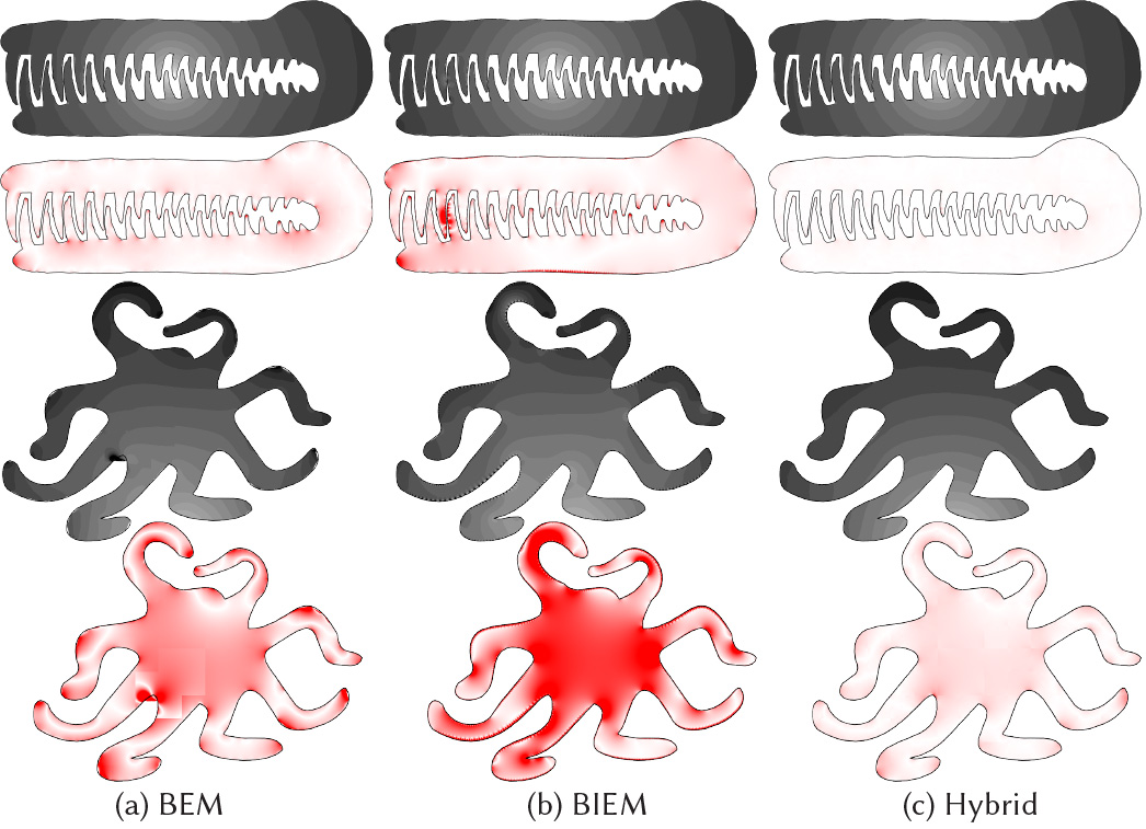
Figure 6. Accuracy comparison between BEM, BIEM, and our Hybrid method. The boundary values are constructed by placing a single source Green’s function in the middle of the figure. The solutions should exactly match the potential induced by that Green’s function. The second and last rows show the error relative to the ground truth, highlighted in red color.

5.1. Comparison between BEM and BIEM

For the comparative analysis between BEM and BIEM, we will divide the diffusion curves algorithm into 3 steps: (1) solution, (2) interpolation, (3) evaluation. BEM uses analytic integration on line segments for solution and evaluation but does not have any interpolation stage. BIEM uses quadrature-based integration for solution and evaluation, and it uses Legendre polynomial interpolation on density values to populate quadrature points for evaluation.

BEM has the limitation that the number of degrees of freedom representing the piecewise constant density $\sigma$ is bounded by the number of elements in the spatial discretization of the boundary curves. BIEM is free from this limitation, and the number of degrees of freedom in the representation of the continous density $\sigma$ is decoupled from the number of quadrature points $e$ used for evaluation. On the other hand, BIEM has the limitation that it is inaccurate when curves are close-to-touching in the solution stage, and has artifacts in the induced potential near the quadrature points in the evaluation stage. BEM, however, is free from both of these problems, since it uses analytic integration along line segments.

5.2. Combination of BEM and BIEM

We propose to combine these two methods, inheriting the strengths of both. We discretize both the solution $\sigma$ and the boundary data $u^{*}$ at Gauss-Legendre nodes, as in BIEM. However, we also introduce the BEM in two places. In order to evaluate integrals of the form Eq. 6 in the solution stage, we interpolate the density using formulas Eq. 13 and Eq. 14 to a BEM-like approximation, which corrects the shortcoming of BIEM for close-to-touching curves. Once we have solved for the solution $\mathring{\bm{\sigma}}$ at the quadrature nodes, we evaluate the potential by once again interpolating to a BEM-like approximation, which corrects the shortcoming of BIEM with respect to artifacts in the induced potential.

We begin by discretizing the boundary data at Gauss-Legendre nodes, leading to the system of equations Eq. 11. We then discretize the boundary curve $S$ into $s$ line segments $\overline{S}_{j}$. If the density values $\overline{\bm{\sigma}}\in\mathbb{R}^{s}$ on these line segments are known, then we can write Eq. 6 as

(17) $$u^{*}(q_{i})=\sum_{j}^{s}\int_{\overline{S}_{j}}G(p,q_{i})dS_{j}(p)\sigma_{j},\quad\text{for each quadrature point $i$}.$$

In matrix form:

(18) $$\mathring{\mathbf{u}}^{*}=\mathring{\overline{\mathbf{G}}}\overline{\bm{\sigma}},$$

Where $\mathring{\mathbf{u}}^{*}\in\mathbb{R}^{g}$ are given boundary values at quadrature points, $\overline{\bm{\sigma}}\in\mathbb{R}^{s}$ are density value on line segments of the boundary, and $\mathring{\overline{\mathbf{G}}}\in\mathbb{R}^{g\times s}$.

Since we choose to discretize the solution $\sigma$ at Gauss-Legendre nodes like in the BIEM, we recover the density values $\overline{\bm{\sigma}}$ by using Legendre polynomial interpolation. Computing the coefficients of the Legendre expansion of $\sigma$ by $\mathbf{c}=\mathring{\mathbf{P}}^{-1}\mathring{\bm{\sigma}}$, we can evaluate the density value on the midpoint of each line segment $\overline{S}_{j}$ by the formula $\overline{\bm{\sigma}}=\overline{\mathbf{P}}\mathbf{c}$ ,where $\overline{\mathbf{P}}\in\mathbb{R}^{s\times g}$ is the Legendre interpolation matrix constructed by evaluating the Legendre polynomials at $\overline{\mathbf{t}}$, which is a vector of curve parameter values corresponding to the midpoints of the line segments $\overline{S}_{j}$. Hence, we have the relation $\overline{\bm{\sigma}}=\overline{\mathbf{P}}\mathring{\mathbf{P}}^{-1}\mathring{\bm{\sigma}}$.

We can thus express our system in matrix form in terms of $\mathring{\bm{\sigma}}$ as:

(19) $$\mathring{\mathbf{u}}^{*}=\underbrace{\mathring{\overline{\mathbf{G}}}\,\overline{\mathbf{P}}\mathring{\mathbf{P}}^{-1}}_{\mathring{\mathbf{G}}_{\textrm{H}}}\mathring{\bm{\sigma}},$$

where $\mathring{\mathbf{G}}_{\textrm{H}}\in\mathbb{R}^{g\times g}$. In order for $\mathring{\mathbf{G}}_{\textrm{H}}$ to have full rank, the number of quadrature points $g$ must be $\leq$ the number of line segments $s$. Note that, regardless of the size of $s$, the dimensionality of the system is $g\times g$. This is beneficial for us, as the matrix that needs to be inverted is much smaller than the corresponding matrix for BEM, $\overline{\mathbf{G}}\in\mathbb{R}^{s\times s}$.

Once we solve the system Eq. 19, we have, by Legendre polynomial interpolation, a density value $\sigma(p)$ that can be evaluated anywhere on the curve. At the evaluation stage, we employ the BEM-like approach of Eq. 10, and now we can use an arbitrary number of line segments $e$, that is independent both of the number line segments $s$ used at solution stage and the number of quadrature points $g$ used to represent the solution. Note that we must use arc length when we integrate over line segments, in order to have consistent integration lengths between the solution and evaluation stages (see the details in Appendix A). We also use arc length parametrization when we construct our BEM-like discretization, so that we have line segments of equal arc length when we subdivide each curve (see the details in Appendix B).

Our method is free from both the visible polyline discretization problem of BEM for a system of the same size, and also from the artifacts around quadrature points that are found in BIEM (see Fig. 4). Our method shows the most accurate results when the number of degrees of freedom in the solution stage and the evaluation stage are both kept fixed (see Fig. 6). In Fig. 4, we set $s=e=4$ for BEM, $g=4,e=20$ for BIEM, and $s=20,g=4,e=20$ for our Hybrid method. In Fig. 6, we set $s=e=8$ for BEM, $g=8,e=40$ for BIEM, and $s=40,g=8,e=40$ for our Hybrid method.

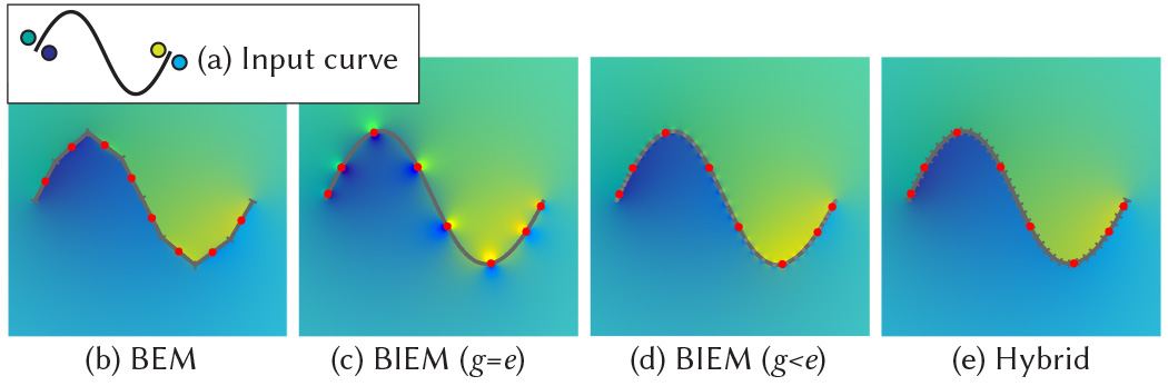
Figure 7. Diffusion curve with double-sided boundary condition given a single Bézier curve (a). Solution comparison with BEM with $s=8$ line segments (b), BIEM with $g=e=8$ (c), BIEM with $g=8,e=40$, and our Hybrid method with $g=8,s=e=40$ (e).

5.3. Double-Sided Boundary Condition

Up to this point, we have been formulating our equations using the single layer potential of Eq. 5 for simplicity of presentation. However, in order to specify two different boundary conditions on each side of an open curve, we must add to our single layer potential representation of Eq. 5 a so-called double layer potential, in which the kernel of Eq. 5 is replaced by $F(p,x)$ from Eq. 4. Our candidate solution is thus represented as

(20) $$u(x)=\int_{S}[G(p,x)\sigma(p)+F(p,x)\mu(p)]dS(p),\forall x\in V.$$

Letting $x$ approach the boundary $S$, we obtain the following BIE:

(21) $$\begin{split}u^{*}_{+}(q)=\int_{S}[G(p,q)\sigma(p)+F(p,q)\mu(p)]dS(p)+\frac{1}{2}\mu(q),\forall q\in S,\\ u^{*}_{-}(q)=\int_{S}[G(p,q)\sigma(p)+F(p,q)\mu(p)]dS(p)-\frac{1}{2}\mu(q),\forall q\in S,\end{split}$$

where the $+$,$-$ subscripts indicate on which side the limit is taken. The terms $\pm\frac{1}{2}\mu(q)$ come from the well-known “jump relations” (Martinsson, 2019) of the double-layer potential (see also Appendix C). Note that the limit process of approaching $x$ to the boundary requires special attention to deal with the problem of singularities in both $G(p,x)$ and $F(p,x)$. (see Appendix C for details). Subtracting these two equations from one another and adding them to one another results in the two equations

(22) $$\begin{split}u^{*}_{+}(q)-u^{*}_{-}(q)=\mu(q),\\ \frac{1}{2}[u^{*}_{+}(q)+u^{*}_{-}(q)]=\int_{S}[G(p,q)\sigma(p)+F(p,q)\mu(p)]dS(p).\end{split}$$

We thus have two equations, which we can solve for the two unknown density functions $\sigma(p)$ and $\mu(p)$. In fact, we see that the value of $\mu(p)$ is given explicitly as the jump $u^{*}_{+}(q)-u^{*}_{-}(q)$.

When BEM is used, the double boundary condition can be expressed in matrix form as:

(23) $$\frac{1}{2}(\overline{\mathbf{u}}^{*}_{+}+\overline{\mathbf{u}}^{*}_{-})=\overline{\mathbf{G}}\overline{\bm{\sigma}}+\overline{\mathbf{F}}\,\overline{\bm{\mu}}.$$

Likewise, when our hybrid method combining BEM and BIEM is used, the double boundary condition can be expressed as:

(24) $$\frac{1}{2}(\mathring{\mathbf{u}}^{*}_{+}+\mathring{\mathbf{u}}^{*}_{-})=\mathring{\mathbf{G}}_{\textrm{H}}\mathring{\bm{\sigma}}+\mathring{\mathbf{F}}_{\textrm{H}}\mathring{\bm{\mu}},$$

where $\mathring{\mathbf{F}}_{\textrm{H}}=\mathring{\overline{\mathbf{F}}}\,\overline{\mathbf{P}}\mathring{\mathbf{P}}^{-1}$, and $\mathring{\bm{\mu}}=\mathring{\mathbf{u}}^{*}_{+}-\mathring{\mathbf{u}}^{*}_{-}$.

This double-sided boundary condition is precisely the condition required to specify the colors on each side of a diffusion curve.

Fig. 7 shows a single diffusion curve example solved with different methods. We used a discretization size of $s=8$ for BEM (b), $g=e=8$ for BIEM (c), $g=8,e=40$ for BIEM (d), and $g=8,s=e=40$ for our Hybrid method (e). Note the visible polyline on BEM, and the dotted-looking artifact on BIEM even for large discretization size (d), whereas our Hybrid method is free from both limitations.

Fig. 8 shows a diffusion curve example of a cherry, with a comparison between FEM, BEM, BIEM and our Hybrid method. We used a discretization size of $s=4$ for BEM and FEM, $g=4,e=20$ for BIEM, and $g=4,s=e=20$ for our Hybrid method.

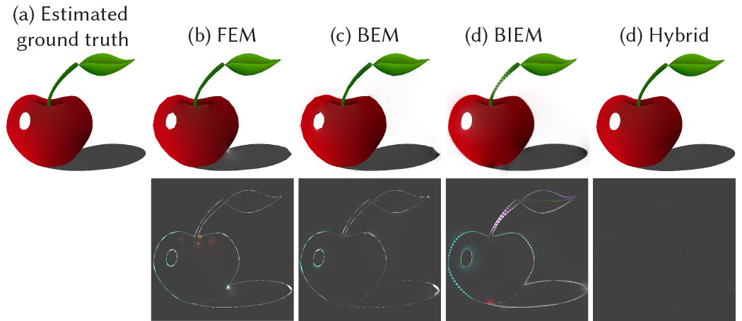
Figure 8. Diffusion curve comparison with FEM, BEM, BIEM and our Hybrid method (top), and its error (bottom) between estimated ground truth, which was achieved by running a dense discretization of BEM ($s=100$ line segments per curve).

5.4. Neumann Boundary Condition

We can also formulate and solve boundary integral equations for Neumann boundary conditions. When a domain $V$ is bounded by a simple closed curve $S$, we can construct a BIE for a Neumann boundary condition on $S$, as follows. Using Green’s third identity, we have the integral representation

(25) $$u(x)=\int_{S}[G(p,x)\psi(p)+F(p,x)u(p)]dS(p),\forall x\in V,$$

where $\psi(p)=\frac{\partial u(p)}{\partial n}$ denotes the Neumann boundary values. Assuming that the Neumann boundary condition is given on the boundary as $\psi=\psi^{*}$, we let $x$ approach the boundary $S$, and obtain the following BIE:

(26) $$u(q)=\int_{S}[G(p,q)\psi^{*}(p)+F(p,q)u(p)]dS(p)+\frac{1}{2}u(q),\forall q\in S\\$$

We can solve this equation for the unknown Dirichlet value on boundary.

In general, if we are given a boundary condition which specifies a combination of Dirichlet boundary values $u^{*}_{d}$ on some parts of the boundary, and Neumann boundary values $\psi^{*}_{n}$ on other parts, then we can solve the following matrix system for $u_{n}$ and $\psi_{d}$:

(27) $$\frac{1}{2}\begin{bmatrix}\mathring{\mathbf{u}}_{d}^{*}\\ \mathring{\mathbf{u}}_{n}\end{bmatrix}=\begin{bmatrix}(\mathring{\mathbf{G}}_{\textrm{H}})_{dd}&(\mathring{\mathbf{G}}_{\textrm{H}})_{dn}\\ (\mathring{\mathbf{G}}_{\textrm{H}})_{nd}&(\mathring{\mathbf{G}}_{\textrm{H}})_{nn}\end{bmatrix}\begin{bmatrix}\mathring{\bm{\psi}}_{d}\\ \mathring{\bm{\psi}}_{n}^{*}\end{bmatrix}+\begin{bmatrix}(\mathring{\mathbf{F}}_{\textrm{H}})_{dd}&(\mathring{\mathbf{F}}_{\textrm{H}})_{dn}\\ (\mathring{\mathbf{F}}_{\textrm{H}})_{nd}&(\mathring{\mathbf{F}}_{\textrm{H}})_{nn}\end{bmatrix}\begin{bmatrix}\mathring{\mathbf{u}}_{d}^{*}\\ \mathring{\mathbf{u}}_{n}\end{bmatrix},$$

where the subscripts $d$,$n$ denote the parts of the boundary on which Dirichlet and Neumann boundary conditions are specificed, respectively. Fig. 5 shows the resulting image when a combination of Dirichlet boundary conditions and Neumann boundary conditions are specified.

Double-sided Neumann boundary conditions on open curves also admit BIE formulations, and can similarly be handled by our Hybrid Method, with the key difference that the BIEs involving double-sided Neumann boundary conditions require the further introduction of an additional hypersingular kernel $H(p,q)$ (see Appendix A.1 of (Liu, 2009)).

5.5. Shortcomings of Brute Force Evaluation

The discussion up to this point provides us with a new method to solve for diffusion curves, one which outperforms the standard BEM in accuracy as demonstrated in Fig. 6, and also shows much better performance (see Table 1) because the system matrix to be solved becomes much smaller.

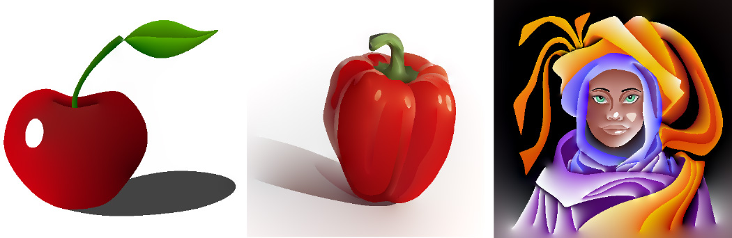
Figure 9. Diffusion curve results generated with our Hybrid Method. All images are in a resolution of $512\times 512$. Examples were taken from (Orzan et al., 2008).

Table 1. Computation time comparison between BEM solve and Hybrid solve for Fig. 9 examples. Once solved, the evaluation step becomes identical if the number of segments are set to be equal.

white		BEM	Hybrid
white	curves	solve	solve	eval
cherry	32	0.10s	0.008s	13.9s
red pepper	109	1.47s	0.079s	64.7s
person with purple cloak	326	32.7s	0.831s	326.7s

However, as shown in Table 1, brute force computation with our Hybrid method still requires an extremely heavy calculation (especially for the evaluation stage, because the number of pixels is much larger). We see then that it is essential to use a fast summation method, such as the Fast Multipole Method (FMM), to achieve reasonable rendering speeds.

6. Fast Solution and Evaluation

The Fast Multipole Method (FMM) is a technique which can be used to rapidly evaluate the potential induced by a collection of $N$ source curves $S$ at a set of $M$ targets $q$:

(28) $$u^{q}=\int_{S}G(p,q)\sigma(p)dS(p).$$

When these potentials are evaluated naively by brute force, the cost grows as $\mathcal{O}(NM)$. With the Fast Multipole Method, this cost is reduced to $\mathcal{O}(KN+KM)$, where the factor $K$ grows logarithmically with the desired accuracy. The key idea behind the FMM is the observation that the potential induced by a collection of sources, when evaluated at a well-separated target, can be represented to high accuracy by a expansion containing only $K$ terms, where the number of terms is independent of the complexity of the source distribution.

We include a complete description of the Fast Multipole Method we implemented to accommodate our use cases in Appendix E. We consider this a reproducibility contribution to the graphics community. Readers unfamiliar with the Fast Multipole Method are strongly encouraged to first read our appendix. FMM is a fairly complicated method, and though many books and previous descriptions exist, we have made a special effort to write a self-contained introduction in terms graphics readers will hopefully better understand. Nevertheless, readers who are willing to treat the FMM as a black box can jump right into Sec. 7 with no loss of continuity. We denote the evaluation of the single-layer integral operator using the FMM by:

(29) $$u^{q}=\mathbf{FMM}_{G}(S,\sigma,q),$$

where $S$ is a collection of source curves, $\sigma$ is a density, and $q$ is a collection of target points.

6.1. Non-Uniform Quadtree

Diffusion curves with the FMM using a uniform quadtree (Sun et al., 2014) becomes inefficient for large domains as it requires a lot of memory for cell allocation as well as significant computation time. Figure 10 compares the use of uniform (perfect) and non-uniform (sparse) quadtrees. We can see that the non-uniform quadtree is much more efficient, allocating a denser quadtree only in regions requiring it.

Please refer to E.5 for a detailed discussion of the technical differences between uniform and non-uniform quadtrees.

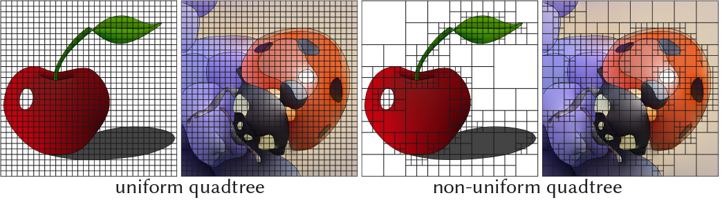
Figure 10. Comparison of a uniform quadtree and a non-uniform quadtree

6.2. Quadtree Clipping

In our discussion of the Fast Multipole Method, we assumed that the curves $S$ were discretized with $M$ degrees of freedom. Suppose that $S$ is discretized with $M$ line segments, and that the integrals over $S$ in the target-from-source, outgoing-from-source, and incoming-from-source formulas are computed using BEM, as described in Section E.1.

At the quadtree construction stage, all cells are subdivided until each cell contains fewer than $b$ degrees of freedom, which in this case means fewer than $b$ line segments. Since the degree of freedom associated with a BEM line segment is located at its midpoint, there will be line segments which span multiple leaf cells in the quadtree, but since the midpoint of such a line segment only belongs to a single cell, this segment is handled by only a single one of the target-from-source, outgoing-from-source, and incoming-from-source formulas. This can result in invalid computations, if, e.g., a part of the line segment that should be handled by the target-from-source formula is handled by the incoming-from-source formula. Such a situation can occur when computing the incoming-from-source terms from the bigger separated list, when a line segment with its midpoint in a cell belonging to the bigger separated list has an endpoint in a cell close to or even inside the target cell. The part of the curve near the endpoint should be computed using the target-from-source formula, but will instead be computed incorrectly by the incoming-from-source formula. In practice, such a situation will indeed occasionally occur, since we are allowing for dramatically different scales and curve sizes in our problem.

This situation is completely remedied by clipping each BEM segment into multiple segments using the quadtree, so that each resulting segment is contained entirely within a single leaf cell (see inset). This ensures that each part of a BEM segment is handled by the correct formula.

6.3. FMM for normal derivative of Green’s function

In previous sections, we described the Fast Multipole Method for rapidly evaluating the single-layer potentials Eq. 5. Suppose instead that we would like to evaluate the double-layer potential with density $\mu$ over the collection of all curves $S$ at all query points $q$:

(30) $$u^{q}=\int_{S}F(p,q)\mu(p)dS(p).$$

It turns out that the Fast Multipole Method for evaluating double-layer potentials is essentially identical to the one presented for single-layer potentials. The only parts of the method that are changed are the target-from-source (see Appendix D.2 and  D.4), outgoing-from-source (see Appendix E.9), and incoming-from-source (see Appendix E.11) operators. We denote this FMM evaluation of the double-layer integral operator by:

(31) $$u^{q}=\mathbf{FMM}_{F}(S,\mu,q).$$

6.4. Precomputations

When the Fast Multipole Method is used to evaluate the potential produced by several different density functions $\sigma$ over a single discretization $\overline{S}$ of a set of curves $S$ and a single set of target points $q$, a large number of computations can be reused between evaluations. Such quantities are independent of the density function, and can be precomputed and stored, in order to accelerate the evaluation of the FMM. The first quantity that can be stored is the quadtree over the discretized source curves $\overline{S}$, which we denote by $\mathcal{Q}$. We denote the function constructing the quadtree over that discretization by

(32) $$\mathcal{Q}=\mathbf{quadtree}(\overline{S}).$$

The next set of quantities which can be precomputed are the various terms that appear in the operators used by the Fast Multipole Method. We denote the collection of precomputed quantities associated with these operators by $\mathcal{P}_{G},\mathcal{P}_{F}$, corresponding to the single-layer and double-layer FMM respectively, and denote the function constructing these quantities by

(33) $$\mathcal{P}_{G},\mathcal{P}_{F}=\mathbf{pre\_FMM}(\overline{S},q,\mathcal{Q}).$$

We describe the precise quantities which are precomputed for each one of the FMM operators in Appendix H.

When these precomputed quantities are available, we can accelerate the FMM by skipping the associated calculations. We indicate that precomputed quantities are used by providing the precomputed quantities as additional arguments to the FMM, writing

(34) $$u^{q}=\mathbf{FMM}_{G}(S,\sigma,q,\mathcal{Q},\mathcal{P}_{G}).$$

6.5. BEM + FMM

In this section, we describe how to combine the BEM, described in Section 4.2, with the FMM, described in Section E.7, in order to rapidly solve and render diffusion curves.

6.5.1. BEM + FMM for solving for unknown density

Suppose that we would like to evaluate a single-layer potential $\sigma$ on a collection of curves $S$ using the boundary element method. We denote the density and curves, discretized into $M$ boundary elements, by $\overline{\bm{\sigma}}$ and $\overline{S}$, respectively. Using the BEM described in Section 4.2, we can evaluate the target-from-source Eq. 79, outgoing-from-source Eq. 80, and incoming-from-source Eq. 83 operators using the discretized density $\overline{\bm{\sigma}}$. If the target points $\overline{{q}}$ are chosen to be same as the source points (the midpoints of the BEM segments, also called the collocation points), then the FMM

(35) $$\overline{\bm{u}}=\mathbf{FMM}_{G}(\overline{S},\overline{\bm{\sigma}},\overline{{q}})$$

provides an $\mathcal{O}(KM)$ algorithm (recalling that $K$ is the number of terms in each expansion) for evaluating the matrix-vector product

(36) $$\overline{\bm{u}}=\overline{\bm{G}}\overline{\bm{\sigma}},$$

described in Section 4.2.

If we are given a desired potential $\overline{\bm{u}}^{*}$ at the BEM collocation points, then we can solve Eq. 9 for the unknown density $\overline{\bm{\sigma}}$ by a direct solver for linear systems, which will have cost $\mathcal{O}(M^{3})$, which is usually prohibitively large. To use the FMM given by Eq. 29 to solve the linear system, we must use a so-called iterative method, which requires only a fast method for evaluating the product of the matrix $\overline{\bm{G}}$ with a vector. If the number of iterations required by the iterative method is small, then the cost will be proportional to the cost of the FMM, $\mathcal{O}(M)$.

One such iterative method is the Generalized Minimum Residuals Method, or GMRES, which solves a linear system $\bm{A}\bm{x}^{*}=\bm{y}^{*}$ for a possibly nonsymmetric matrix $\bm{A}$, and which minimizes the residual $\|{\bm{A}\bm{x}-\bm{y}^{*}}\|$, where $\bm{x}\approx\bm{x}^{*}$ is the approximate solution computed by GMRES. To indicate that the GMRES method is used to solve the linear system $\bm{A}\bm{x}=\bm{y}$ to within an error of $\epsilon$ in the residual, where $f(\cdot)$ is a function approximating the matrix-vector product $f(\bm{x})\approx\bm{A}\bm{x}$, and where $\bm{x}_{0}$ is the initial guess for the solution, we write

(37) $$\bm{x}=\mathbf{GMRES}(f(\cdot),\bm{x}_{0},\bm{y},\epsilon).$$

Thus, to solve for the unknown density $\overline{\bm{\sigma}}$ in Eq. 9 using the FMM, we compute

(38) $$\overline{\bm{\sigma}}=\mathbf{GMRES}(\mathbf{FMM}_{G}(\overline{S},(\cdot),\overline{q}),\overline{\bm{\sigma}}_{0},\overline{\bm{u}}^{*},\epsilon),$$

using a random initial guess $\overline{\bm{\sigma}}_{0}$. (we typically choose $\overline{\bm{\sigma}}_{0}=\overrightarrow{1}$)

6.5.2. BEM + FMM for double-sided boundary condition

If a double sided boundary condition is given, like the one described in Section 5.3, we need to solve for unknown density $\overline{\bm{\sigma}}$ in Eq. 23. In other words, given a discretized curve $\overline{S}$ and boundary conditions $\overline{\bm{u}}^{*}_{+}$ and $\overline{\bm{u}}^{*}_{-}$ on each side, we must solve for $\overline{\bm{\sigma}}$ in

(39) $$\frac{1}{2}(\overline{\mathbf{u}}^{*}_{+}+\overline{\mathbf{u}}^{*}_{-})=\overline{\mathbf{G}}\overline{\bm{\sigma}}+\overline{\mathbf{F}}\,\overline{\bm{\mu}},$$

where $\overline{\bm{\mu}}=\overline{\bm{u}}^{*}_{+}-\overline{\bm{u}}^{*}_{-}$.

Using the FMM, we can rapidly solve for $\overline{\bm{\sigma}}$, as follows. First, we compute a right hand side vector $\bm{b}$ by the computation

(40) $$\mathbf{b}=\frac{1}{2}(\overline{\mathbf{u}}^{*}_{+}+\overline{\mathbf{u}}^{*}_{-})-\mathbf{FMM}_{F}(\overline{S},\overline{\bm{\mu}},\overline{q}).$$

Next, we solve for $\overline{\bm{\sigma}}$ using GMRES:

(41) $$\overline{\bm{\sigma}}=\mathbf{GMRES}(\mathbf{FMM}_{G}(\overline{S},(\cdot),\overline{q}),\overline{\bm{\sigma}}_{0},\mathbf{b},\epsilon),$$

using a random initial guess $\overline{\bm{\sigma}}_{0}$. The total cost of this computation will be $\mathcal{O}(M)$, where $M$ is the number of BEM segments used.

To improve things further, we can precompute the quantities needed by the FMM, as described in Section 6.4. The full algorithm for solving for a double-sided boundary condition using the FMM and BEM is described in Algorithm 1.

Algorithm 1 FMM + BEM for Solving

Input: source curves $\overline{S}$, collocation points $\overline{q}$, boundary values $\overline{\bm{u}}^{*}_{+},\overline{\bm{u}}^{*}_{-}$, initial guess for density $\overline{\bm{\sigma}}_{0}$

Output: density values $\overline{\bm{\sigma}}$, quadtree $\mathcal{Q}$, precomputed values $\mathcal{P}_{G}$, $\mathcal{P}_{F}$

1:$\mathcal{Q}=\mathbf{quadtree}(\overline{S})$

2:$\mathcal{P}_{G},\mathcal{P}_{F}=\mathbf{pre\_FMM}(\overline{S},\overline{q},\mathcal{Q})$

3:Set $\overline{\bm{\mu}}=\overline{\bm{u}}^{*}_{+}-\overline{\bm{u}}^{*}_{-}$

4:$\mathbf{b}=\frac{1}{2}(\overline{\bm{u}}^{*}_{+}+\overline{\bm{u}}^{*}_{-})-\mathbf{FMM}_{F}(\overline{S},\overline{\bm{\mu}},\overline{q},\mathcal{Q},\mathcal{P}_{F})$

5:$\overline{\bm{\sigma}}=\mathbf{GMRES}(\mathbf{FMM}_{G}(\overline{S},(\cdot),\overline{q},\mathcal{Q},\mathcal{P}_{G}),\overline{\bm{\sigma}}_{0},\mathbf{b},\epsilon)$

6.5.3. Diffusion Curve with BEM + FMM

The overall algorithm for using the BEM and FMM to compute pixel values $u^{q}$ at all pixels $q$ on 2D domain, given a set of discretized diffusion curves $\overline{S}$ with collocation points $\overline{\bm{q}}$, and a double-sided boundary condition $\overline{\bm{u}}^{*}_{+}$ and $\overline{\bm{u}}^{*}_{-}$, is as follows:

Algorithm 2 Diffusion Curve with FMM + BEM

Input: source curves $\overline{S}$, collocation points $\overline{q}$, pixel targets $q$, boundary values $\overline{\bm{u}}^{*}_{+},\overline{\bm{u}}^{*}_{-}$, initial guess for density $\overline{\bm{\sigma}}_{0}$

Output: target pixel values: $u^{q}$

1:Use Algorithm 1 to solve for the density of the single layer $\overline{\bm{\sigma}}$ at the collocation points $\overline{q}$, using the inputs $(\overline{S},\overline{q},\overline{\bm{u}}^{*}_{+},\overline{\bm{u}}^{*}_{-})$

2:Set $\overline{\bm{\mu}}=\overline{\bm{u}}^{*}_{+}-\overline{\bm{u}}^{*}_{-}$

3:$u^{q}=\mathbf{FMM}_{G}(\overline{S},\overline{\bm{\sigma}},q,\mathcal{Q},\mathcal{P}_{G})+\mathbf{FMM}_{F}(\overline{S},\overline{\bm{\mu}},q,\mathcal{Q},\mathcal{P}_{F})$

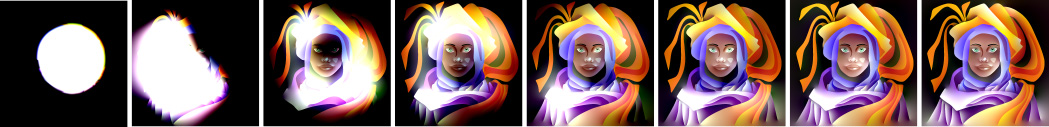
Figure 11. Visualization of the first few iterations of GMRES

6.6. Hybrid Method + FMM

In this section, we describe how to combine our Hybrid Method, described in Section 5, with the FMM, described in Section E.7, in order to rapidly solve and render diffusion curves.

6.6.1. Hybrid Method + FMM for double-sided boundary condition

When the FMM is combined with BEM for solving for an unknown density with a double-sided boundary condition (see Section 6.5.2), the target points $\overline{q}$ coincide with the collocation points on the discretized curves $\overline{S}$:

(42) $$\overline{\bm{u}}=\mathbf{FMM}_{G}(\overline{S},\overline{\bm{\sigma}},\overline{q}).$$

On the other hand, when the Hybrid Method is used, the density $\sigma$ is represented at $g$ Gauss-Legendre nodes $\mathring{q}$, and this discretized density is written as $\mathring{\bm{\sigma}}$ (see Section 5). The potential at these quadrature nodes $\mathring{q}$ is evaluated using the BEM, where the curve $S$ is descretized into $s$ line segments $\overline{S}$, with $s>g$. The density $\mathring{\bm{\sigma}}$ is interpolated to the $s$ BEM collocation points by the formula $\overline{\bm{\sigma}}=\overline{\mathbf{P}}\mathring{\mathbf{P}}^{-1}\mathring{\bm{\sigma}}$. The potential created by the density $\mathring{\bm{\sigma}}$ can thus be evaluated at the points $\mathring{q}$ using the calculation

(43) $$\mathring{\bm{u}}=\mathbf{FMM}_{G}(\overline{S},\overline{\bm{P}}\mathring{\bm{P}}^{-1}\mathring{\bm{\sigma}},\mathring{q}).$$

This is an $\mathcal{O}(s)$ algorithm for evaluating the matrix-vector product

$$\mathring{\mathbf{u}}=\underbrace{\mathring{\overline{\mathbf{G}}}\,\overline{\mathbf{P}}\mathring{\mathbf{P}}^{-1}}_{\mathring{\mathbf{G}}_{\textrm{H}}}\mathring{\bm{\sigma}},$$

where $\mathring{\overline{\mathbf{G}}}\in\mathbb{R}^{g\times s}$ and $\mathring{\mathbf{G}}_{\textrm{H}}\in\mathbb{R}^{g\times g}$.

The FMM + BEM method for solving for an unknown density with double-sided boundary conditions can thus be reformulated using the Hybrid Method, as follows:

Algorithm 3 FMM + Hybrid Method for Solving

Input: source curves $\overline{S}$, quadrature nodes $\mathring{q}$, boundary values $\mathring{\bm{u}}^{*}_{+},\mathring{\bm{u}}^{*}_{-}$, initial guess for density $\mathring{\bm{\sigma}}_{0}$

Output: density values $\mathring{\bm{\sigma}}$, quadtree $\mathcal{Q}$, precomputed values $\mathcal{P}_{G}$, $\mathcal{P}_{F}$

1:$\mathcal{Q}=\mathbf{quadtree}(\overline{S})$

2:$\mathcal{P}_{G},\mathcal{P}_{F}=\mathbf{pre\_FMM}(\overline{S},\mathring{q},\mathcal{Q})$

3:Set $\mathring{\bm{\mu}}=\mathring{\bm{u}}^{*}_{+}-\mathring{\bm{u}}^{*}_{-}$

4:$\mathbf{b}=\frac{1}{2}(\mathring{\mathbf{u}}^{*}_{+}+\mathring{\mathbf{u}}^{*}_{-})-\mathbf{FMM}_{F}(\overline{S},\overline{\mathbf{P}}\mathring{\mathbf{P}}^{-1}\mathring{\bm{\mu}},\mathring{q},\mathcal{Q},\mathcal{P}_{F})$

5:$\mathring{\bm{\sigma}}=\mathbf{GMRES}(\mathbf{FMM}_{G}(\overline{S},\overline{\mathbf{P}}\mathring{\mathbf{P}}^{-1}(\cdot),\mathring{q},\mathcal{Q},\mathcal{P}_{G}),\mathring{\bm{\sigma}}_{0},\mathbf{b},\epsilon)$

With the Hybrid Method, the dimensionality of the unknown density is much smaller than for the standard BEM, and the number of BEM segments $s$ used can also be smaller than for the standard BEM. Hence, the FMM evaluation step above is much faster. Furthermore, since the number of degrees of freedom in the discretization is smaller, the number of iterations of GMRES is much smaller as well. This is because we are solving an integral equation involving a single-layer potential, and the condition number of such a system grows with the number of degrees of freedom in the discretization. Fig. 11 visualizes the first few iterations of GMRES.

6.6.2. Diffusion Curve with Hybrid Method + FMM

The overall algorithm for using the Hybrid Method, together with the FMM, to compute pixel values $u^{q}$ at all pixels $q$ on 2D domain, given a set of discretized diffusion curves $\overline{S}$ with quadrature points $\mathring{q}$, and a double-sided boundary condition $\mathring{\bm{u}}^{*}_{+}$ and $\mathring{\bm{u}}^{*}_{-}$, is as follows:

Algorithm 4 Diffusion Curve with FMM + Hybrid Method

Input: source curves $\overline{S}$, quadrature points $\mathring{q}$, pixel targets $q$, boundary values $\mathring{\bm{u}}^{*}_{+},\mathring{\bm{u}}^{*}_{-}$, initial guess for density $\mathring{\bm{\sigma}}_{0}$

Output: target pixel values: $u^{q}$

1:Use Algorithm 3 to solve for the density of the single layer $\mathring{\bm{\sigma}}$ at the quadrature nodes $\mathring{q}$, using the inputs $(\overline{S},\mathring{q},\mathring{\bm{u}}^{*}_{+},\mathring{\bm{u}}^{*}_{-})$

2:Set $\mathring{\bm{\mu}}=\mathring{\bm{u}}^{*}_{+}-\mathring{\bm{u}}^{*}_{-}$

3:$u^{q}=\mathbf{FMM}_{G}(\overline{S},\overline{\mathbf{P}}\mathring{\mathbf{P}}^{-1}\mathring{\bm{\sigma}},q,\mathcal{Q},\mathcal{P}_{G})+\mathbf{FMM}_{F}(\overline{S},\overline{\mathbf{P}}\mathring{\mathbf{P}}^{-1}\mathring{\bm{\mu}},q,\mathcal{Q},\mathcal{P}_{F})$

6.7. Need for Adaptive Subdivision

The discussion up to this point provides us with an FMM to solve for diffusion curves with the Hybrid Method that we introduced in Sec. 5. Fig. 12 shows the results of several examples generated with the Hybrid Method + FMM and its corresponding computation time in Table 2

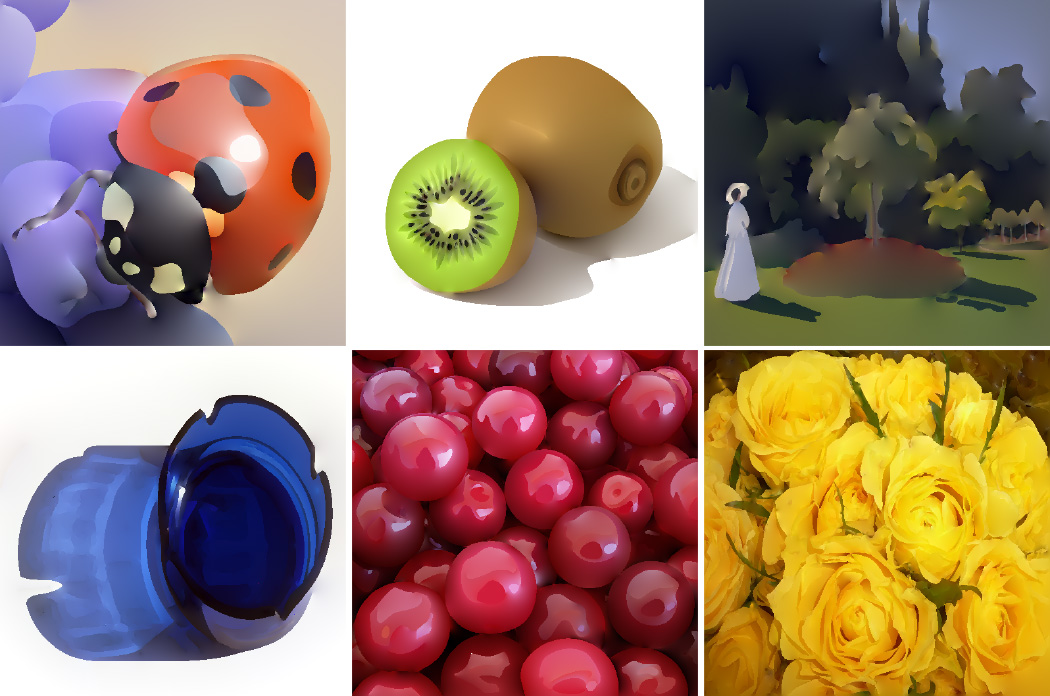
Figure 12. Diffusion curve results generated with our Hybrid Method + FMM. All images are in a resolution of $512\times 512$. Lady bug, blue glass, and yellow roses examples were taken from (Orzan et al., 2008); kiwi and Monet examples were taken from (Jeschke et al., 2011); cherries example was taken from (Sun et al., 2014).

Table 2. Computation time comparison between brute force and FMM for above Fig. 12 examples (N\A: cherries and yellow roses examples hung in the evaluation stage).

white		Brute		FMM
white	curves	solve	eval	solve	eval
ladybug	151	0.14s	133s	0.33s	0.41s
kiwi	330	0.82s	355s	0.59s	0.81s
monet	423	1.43s	429s	0.53s	0.58s
blue glass	525	2.42s	519s	0.53s	0.68s
cherries	1110	17.26s	N\A	3.55s	0.95s
yellow roses	4632	1126s	N\A	10.49s	1.8s

If the given discretization is not sufficient to represent the given diffusion curve, as shown in left of Fig. 13, or if the user performs an extreme zoom-in of small region, as demonstrated in Fig. 1, we need to employ an adaptive subdivision strategy to ensure accurate evaluation.

7. Adaptive Strategy for Infinite Resolution

To create an infinite resolution image representation, we adopt the following adaptive strategy. In our Hybrid Method (see Section 5), there are three discretization parameters that we have control over: $g$, the number of quadrature nodes; $s$, the number of BEM line segments used to discretize the source curves during the solution step; and $e$, the number of BEM segments used to discretize the curves in the evaluation step.

On the one hand, the number of quadrature nodes $g$ must be large enough so that the single layer density $\sigma$ solving the double-sided boundary value problem is well-represented. In other words, we would like $g$ to be large enough so the Legendre expansions associated with the quadrature nodes accurately represent $\sigma$. The number of BEM segments $s$ in the solving step should also be large enough to resolve the potential at all of the quadrature nodes, and, in practice, this is achieved when $s$ is a constant multiple of $g$ (we discuss this in the sequel). The number of discretization nodes $g$ and $s$ thus depend solely on the smoothness of the solution $\sigma$, and the desired accuracy of approximation.

On the other hand, the number of BEM segments $e$ used in the evaluation stage must be large enough so that the layer potentials in the final image look smooth and continuous. This depends on the particular part of the image the user is requesting to view, called the viewport, as well as the pixel resolution that the user is requesting.

The key idea behind our adaptive strategy is to select the optimal number of quadrature nodes $q$ and BEM segments for the solution stage $s$ separately from the number of evaluation BEM segments $e$. This is made possible by the interpolation formula described in Section 5.2, which allows us to interpolate a density known at Gauss-Legendre nodes to its values at arbitrarily many BEM segments. Since the optimal number of quadrature nodes $q$ will be significantly smaller than the number of evaluation BEM segments $e$, this will result is a dramatic reduction of cost in the solution stage. Furthermore, since the density can be interpolated to any number of BEM segments, this means that it is possible to change the viewport and pixel density without re-solving the equations for the density, which gives us an efficient infinite resolution zoom.

In Section 7.1, we describe the optimal strategy for selecting the number of quadrature nodes $q$, and their locations. In Section 7.2, we describe a strategy for selecting the number of BEM segments $s$ and $e$. Finally, in Section 7.4, we describe a strategy for updating our discretization based on the user’s requested viewport and pixel resolution.

Figure 13. An initial input curve with its resulting color values (left), and the same curve subdivided, with its resulting color values (right).

7.1. Adaptive Subdivision

The number of quadrature points needed to represent the density $\sigma$ on any particular curve will need to be larger if the associated double sided boundary condition is complicated, if the curve has an intricate geometry (e.g. a shape with high curvature), or if the curve has many other curves nearby. The relationship between the number of required quadrature nodes and this a priori information can be somewhat complicated, so instead of using this a priori information directly, we opt to use a simpler condition depending only on the density itself.

If we are able to quickly determine whether or not a particular set of quadrature points has adequately represented the density, then, by repeatedly adding more degrees of freedom to any underresolved curve, we can achieve an optimal discretization of $\sigma$. There are two ways of adding degrees of freedom to a curve: by choosing a higher-order Gauss-Legendre quadrature, or by subdividing the curve into two sub-curves, and keeping the order of the quadrature on each curve the same. Of the two approaches, the latter is more stable, since increasing the order of the quadrature can cause the quadrature points to cluster excessively, leading to an increase in the condition number of the Green’s function matrix. In our examples, we subdivide the curve while keeping the number of quadrature points on each curve equal to $4$.

To determine whether a panel on a curve needs subdivision, we examine the size of the highest order expansion coefficient of the Legendre polynomial expansion of the density. A large value in the highest order coefficient means that the density function requires more degrees of freedom to be properly resolved. Hence, we subdivide the curve if the highest order coefficient of the Legendre polynomial expansion is larger than a threshold, which is set globally independent of the domain. This approach works for any smooth density, however, if the true density is singular (near a corner, for example), then this strategy can result in an infinite number subdivisions if we don’t provide any constraint on the smallest size of the resulting curves. Thus, we ensure that further subdivision isn’t performed if the length of the curve is below a second threshold, which is dependent on the size of the viewport domain. The overall algorithm can be described as follows:

Algorithm 5 Adaptive Subdivision

1:loop  over every curve:

2:     if length of curve ¡ $\epsilon_{1}$ (depends on size of pixel)  then

3:         skip      

4:     if highest order coefficient of Legendre polynomial expansion ¿ $\epsilon_{2}$ (global) then

5:         subdivide curve      

If a collection of curves is determined to need subdivision, then their density values need to be re-solved. Fig. 13 shows the initial bleeding artifact being fixed with our adaptive subdivision algorithm, combined with a re-solving for the density values (note that subdivision is only applied on a sharp corner of the curve with an abrupt color change). We accelerate the process of re-solving for the subdivided densities by the techniques described in the following subsections.

7.1.1. Warm start of density value

When re-solving for density values, it is necessary to re-run GMRES with the FMM (see Section 6.5.1). However, instead of re-solving for the density values $\mathring{\bm{\sigma}}$ from scratch, we can instead specify an initial guess $\mathring{\bm{\sigma}}_{0}$ from the previous solution, by interpolating the old density to the quadrature nodes on the subdivided curves. This significantly reduces the number of iterations required by GMRES.

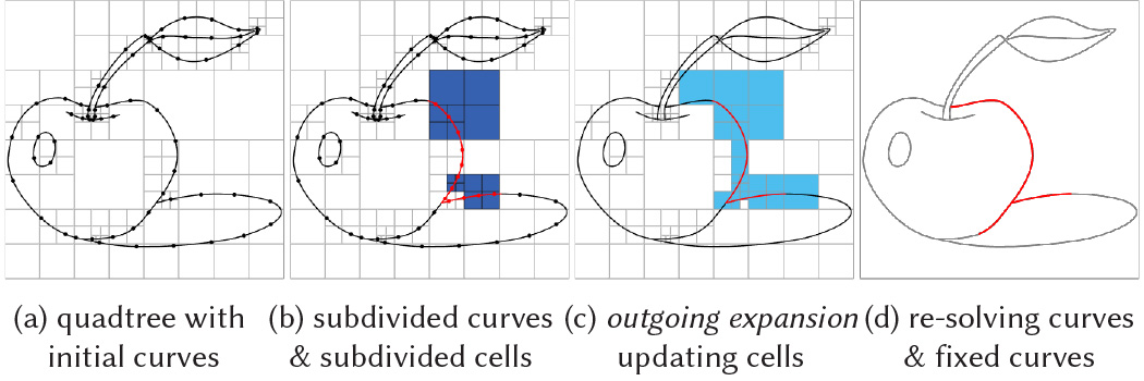
Figure 14. An initial quadtree is generated from an initial curve (a). Subdivided curves appear, causing some of cells to further subdivide to satisfy the condition on the minimum number of segments per cell (b) (Section 7.1.2). For every cell that includes subdivided curves, we update its outgoing expansion (c) (Section 7.1.3). Re-solving curves are determined by perturbing the density value on each subdivided curve (d) (Section 7.1.4).

7.1.2. Local update of quadtree

Instead of re-constructing the quadtree every time a curve panel is subdivided, we can update the already pre-constructed quadtree $\mathcal{Q}$, so that we can re-use the pre-computed expansions $\mathcal{P}_{G}$ (see Section 6.4). Recall that the quadtree is constructed by repeatedly subdividing cells, until each cell contains fewer than $b$ degrees of freedom. To update the quadtree, we check the prescribed condition on the maximum number of BEM line segments in each cell and, whenever it is violated after curve subdivision, the containing cell is subdivided until the prescribed condition is satisfied (see Fig.  14 (b)). Note that, whenever the quadtree is updated, the cell relationships described in the various lists (the neighbor list, the interaction list, etc.) also need to be updated. These lists can also be locally updated by only considering newly generated cells or any cells that contain newly generated cells in their relations. We denote the local update of the quadtree by

(44) $$\mathcal{Q}^{\prime}=\mathbf{update\_quadtree}(\overline{S}^{\prime},\mathcal{Q}),$$

where $\mathcal{Q}$ is the quadtree constructed for the old set of discretized curves $\overline{S}$, and where $\overline{S}^{\prime}$ and $\overline{\mathcal{Q}}^{\prime}$ denote the updated curves and updated quadtree, respectively.

7.1.3. Local update of expansions

The pre-computed expansion information from the pre-computation step $\mathcal{P}_{G}=\mathbf{pre\_FMM}_{G}(\overline{S},\mathring{q},\mathcal{Q})$ can be also locally updated while preserving some of the previously computed information. We denote the operator updating the precomputed information by

(45) $$\mathcal{P}_{G}^{\prime}=\mathbf{update\_pre\_FMM}_{G}(\overline{S}^{\prime},\mathring{q}^{\prime},\mathcal{Q}^{\prime},\mathcal{P}_{G}),$$

where $\overline{S}^{\prime}$, $\mathring{q}^{\prime}$, and $\mathcal{Q}^{\prime}$ are the updated discretized curves, quadrature nodes, and quadtree respectively.

Determining which cells have precomputations that need to be updated depends on the particular precomputation being considered. For the outgoing-from-source operator, only the leaf cells that have a change in their contained line segments need to be updated (see Fig.  14 (c)). For the outgoing-from-outgoing operator, cells that have a child cell that has been updated need to be updated accordingly. For the incoming-from-outgoing operator, the cells that have had a change in their interaction list need to be updated. For the incoming-from-source operator, the cells that have any change on their bigger separated list need to updated. For the incoming-from-incoming operator, essentially all cells will need updating, since the upward and downward process of the FMM will eventually touch every cell. Similarly, the target-from-incoming operator will require updates on every cell. For the target-from-outgoing operator, the cells that have any change on their seperated list need to be updated, and for the target-from-source operator, those cells that have any change on their adjacency list, or any change on their own cells, need to be updated. All newly generated cells will also obviously need to constuct every pre-computation for each of the FMM operators.

7.1.4. Local re-solve of density value

When some curves are subdivided, the density does not necessarily have to be updated everywhere. The density on curves with subdivided panels must naturally be updated, as well as the density on nearby curves which might be affected by this subdivision. Curves that are far away may not need updating at all.

We use the following method to determine which curves are in need of re-solving. We run the FMM separately on each of the newly subdivided curves $S_{\alpha}\in\overline{S}^{\prime}$, using a density $\overline{\bm{\rho}}$ that is given the value one on the subdivided $S_{\alpha}$, and is given the value zero on all other curves:

(46) $$\mathring{\bm{v}}=\mathbf{FMM}_{G}(\overline{S}^{\prime},\overline{\bm{\rho}},\mathring{q}^{\prime},\mathcal{Q}^{\prime},\mathcal{P}_{G}^{\prime})$$

where $\overline{S}^{\prime}$, $\mathring{q}^{\prime}$, $\mathcal{Q}^{\prime}$, and $\mathcal{P}_{G}^{\prime}$ are the updated discretized curves, quadrature nodes, quadtree, and precomputations, respectively. We use the resulting output potential $\mathring{\bm{v}}$ to determine which curves are influenced most by the subdivision. Intuitively, this can be seen as perturbing the density value with a unit charge on each subdivided curve to check for its effect on other curves. We then determine which other curves need to be updated, by the following procedure. First, we determine how much the induced potential changes over the subdivided curve $S_{\alpha}$ by computing the quantity $\max\mathring{\bm{v}}_{S_{\alpha}}-\min{\mathring{\bm{v}}_{S_{\alpha}}}$. We then find all curves $S_{\beta}$ in need of re-solving by checking if the change in the induced potential $\max\mathring{\bm{v}}_{S_{\beta}}-\min{\mathring{\bm{v}}_{S_{\beta}}}$ is greater than $0.9$ times the change over $S_{\alpha}$. In other words, a curve $S_{\beta}$ is determined to be in need of re-solving if

(47) $$\max\mathring{\bm{v}}_{S_{\beta}}-\min{\mathring{\bm{v}}_{S_{\beta}}}>0.9(\max\mathring{\bm{v}}_{S_{\alpha}}-\min{\mathring{\bm{v}}_{S_{\alpha}}}).$$

We label all such curves as the re-solving curves (see Fig.  14 (d)). One of the reasons that this scheme works so well in practice is that the mean-value theorem tells us that the change in the induced potential over the curve is related to the integral of the derivative of the potential. The potential induced by the kernel $G(p,q)$ is proportional to $\log(\|p-q\|)$ and decays very slowly, and does not provide a good measure for identifying nearby re-solving curves. On the other hand, its derivative $F(p,q)$ is proportional to $1/\|p-q\|$ and decays much more quickly, and provides an excellent measure for identifying nearby curves.

The extra step of potential evaluation for each subdivided curve $S_{\alpha}$ needed to identify the re-solving curves saves a great amount of computation in the end, because it reduces the dimensionality of the linear system we must solve for the new density value, which needs to be computed using several steps of FMM evaluation within GMRES. In fact, it is not necessary to compute the full FMM in Eq. 46, since, as we describe later in this section, a more efficient local FMM can be performed instead.

After we have determined the re-solving curves, we only need to re-solve for the density on the re-solving curves, while leaving the density on the remaining curves, which we call the constrained curves, unchanged. We denote the set of re-solving curves by $r\subset S$, and the set of constrained curves by $c\subset S$. We then denote the quadrature nodes on the resolving curves by $\mathring{q}_{r}^{\prime}$, and the quadrature nodes on the constrained curves by $\mathring{q}_{c}$. Likewise, we denote the BEM segments on the re-solving curves by $\overline{q}_{r}^{\prime}$ and on the constrained curves by $\overline{q}_{c}$ (omitting the $(\cdot)^{\prime}$ from the constained curves, since the nodes and BEM segments on those curves are unchanged). We represent the above procedure for determining which curves are re-solving curves and which are constrained curves by

(48) $$r,c=\mathbf{label\_curves}(\overline{S}^{\prime},\mathring{q}^{\prime},\mathcal{Q}^{\prime},\mathcal{P}_{G}^{\prime}),$$

where $\overline{S}^{\prime}$, $\mathring{q}^{\prime}$, $\mathcal{Q}^{\prime}$, and $\mathcal{P}_{G}^{\prime}$ are the updated discretized curves, quadrature nodes, quadtree, and precomputations, respectively.

7.1.5. Accelerating the local re-solve

Since the density is unchanged on all of the constrained curves, we can solve a much smaller linear system than we would if we were solving for the density from scratch. Let’s first formulate this problem with a matrix system so that we have clear idea what we want to achieve, and then reformuate the problem using the FMM. Recall that, using our Hybrid Method, the unknown density $\mathring{\bm{\sigma}}^{\prime}$ is the solution to the linear system

(49) $$\mathring{\mathbf{G}}_{\textrm{H}}\mathring{\bm{\sigma}}^{\prime}=\mathring{\bm{b}}^{*^{\prime}},$$

for some right hand side ${\bm{b}^{*}}^{\prime}$, where $\mathring{\mathbf{G}}_{\textrm{H}}=\mathring{\overline{\mathbf{G}}}\,\overline{\mathbf{P}}\mathring{\mathbf{P}}^{-1}\in\mathbb{R}^{g\times g}$, and $\mathring{\overline{\mathbf{G}}}\in\mathbb{R}^{g\times s}$ (see Section 5.2). Solving for the potential only at the quadrature nodes $\mathring{q}_{r}^{\prime}$ on the re-solving curves, while constraining the density at the quadrature nodes $\mathring{q}_{c}$ on the constrained curves, gives us the linear system

(50) $$\begin{bmatrix}(\mathring{\mathbf{G}}_{\textrm{H}})_{rr}&(\mathring{\mathbf{G}}_{\textrm{H}})_{rc}\\ \end{bmatrix}\begin{bmatrix}\mathring{\bm{\sigma}}_{r}^{\prime}\\ \mathring{\bm{\sigma}}_{c}\end{bmatrix}=\mathring{\bm{b}}^{*^{\prime}}_{r}$$

Then, setting $\mathring{\bm{\sigma}}_{c}$ to the previously solved value and placing it on right hand side:

(51) $$(\mathring{\mathbf{G}}_{\textrm{H}})_{rr}\mathring{\bm{\sigma}}_{r}^{\prime}=\mathring{\bm{b}}^{*^{\prime}}_{r}-(\mathring{\mathbf{G}}_{\textrm{H}})_{cr}\mathring{\bm{\sigma}}_{c}.$$

To solve this equation with the FMM, we compute:

(52) $$\mathring{\bm{b}}^{\#^{\prime}}_{r}=\mathring{\bm{b}}^{*^{\prime}}_{r}-\mathbf{FMM}_{G}(\overline{S}_{c},\overline{\mathbf{P}}\mathring{\mathbf{P}}^{-1}\mathring{\bm{\sigma}}_{c},\mathring{q}_{r}^{\prime}),$$

and then solve for $\mathring{\bm{\sigma}}_{r}^{\prime}$ using GMRES:

(53) $$\mathring{\bm{\sigma}}_{r}^{\prime}=\mathbf{GMRES}(\mathbf{FMM}_{G}(\overline{S}_{r}^{\prime},\overline{\mathbf{P}}\mathring{\mathbf{P}}^{-1}(\cdot),\mathring{q}_{r}^{\prime}),(\mathring{\bm{\sigma}}_{r}^{\prime})_{0},{\mathring{\bm{b}}^{\#^{\prime}}}_{r},\epsilon),$$

where $(\mathring{\bm{\sigma}}_{r}^{\prime})_{0}$ is the initial guess for $\mathring{\bm{\sigma}}_{r}^{\prime}$ at the updated quadrature nodes $\mathring{q}^{\prime}_{r}$.

While we can use the FMM to compute the potentials created by densities on the constrained curves $S_{c}$ and the resolving curves $S_{r}^{\prime}$ from scratch, we can dramatically accelerate the calculations by using the fact that the $S_{c}$ and $S_{r}^{\prime}$ are subsets of the updated curves $S^{\prime}$, for which we already have an updated quadtree $\mathcal{Q}^{\prime}$ and updated precomputations $\mathcal{P}_{G}^{\prime}$. We thus define the following modified FMM, for performing local calculations that take advantage of precomputations on a larger set of curves and targets.

Suppose that $\mathcal{Q}$ and $\mathcal{P}_{G}$ are the quadtree and precomputations for the FMM with source curves $S$ and targets $q$. We define the FMM

(54) $$u^{q}=\mathbf{local\_FMM}_{G}(\widetilde{S},\sigma,\widetilde{q},\mathcal{Q},\mathcal{P}_{G})$$

for computing the potential created by a subset $\widetilde{S}\subset{S}$ of source curves at a subset $\widetilde{q}\subset q$ of target points, by modifying the outgoing-from-source, incoming-from-source, target-from-incoming, target-from-outgoing, and target-from-source operators (see Section E.1), as follows. First, the two operators used to construct outgoing expansions and incoming expansions from sources are modified to only use the source curves $\widetilde{S}$. The last three operators used to compute potentials at the targets are modified to only compute the potentials at the points $\widetilde{q}$. Note that the operators for translating expansions can remain unchanged from Algorithm 8.

Finally, using this local FMM, we can find the solution to the system Eq. 51 for the density $\mathring{\bm{\sigma}}_{r}^{\prime}$ on the re-solving curves, by first computing

(55) $$\mathring{\bm{b}}^{\#^{\prime}}_{r}=\mathring{\bm{b}}^{*^{\prime}}_{r}-\mathbf{local\_FMM}_{G}(\overline{S}_{c},\overline{\mathbf{P}}\mathring{\mathbf{P}}^{-1}\mathring{\bm{\sigma}}_{c},\mathring{q}_{r}^{\prime},\mathcal{Q}^{\prime},\mathcal{P}_{G}^{\prime}),$$

and then solving for $\mathring{\bm{\sigma}}_{r}^{\prime}$ using GMRES:

(56) $$\mathring{\bm{\sigma}}_{r}^{\prime}=\mathbf{GMRES}(\mathbf{local\_FMM}_{G}(\overline{S}_{r}^{\prime},\overline{\mathbf{P}}\mathring{\mathbf{P}}^{-1}(\cdot),\mathring{q}_{r}^{\prime},\mathcal{Q}^{\prime},\mathcal{P}_{G}^{\prime}),(\mathring{\bm{\sigma}}_{r}^{\prime})_{0},{\mathring{\bm{b}}^{\#^{\prime}}}_{r},\epsilon),$$

where $(\mathring{\bm{\sigma}}_{r}^{\prime})_{0}$ is the initial guess for $\mathring{\bm{\sigma}}_{r}^{\prime}$ at the updated quadrature nodes $\mathring{q}^{\prime}_{r}$.

7.1.6. Local update for adaptive subdivision

The overall algorithm for locally re-solving for the density on the re-solving curves can be described as follows:

Algorithm 6 Local Re-solve after Curve Subdivision

Input: source curves $\overline{S}$, quadrature nodes $\mathring{q}$, right hand side $\mathring{\bm{b}}^{*}$, previous density $\mathring{\bm{\sigma}}$, sources curves after subdivision $\overline{S}^{\prime}$, quadrature nodes after subdivision $\mathring{q}^{\prime}$

Output: updated density value $\mathring{\bm{\sigma}}^{\prime}$

1:$\mathcal{Q}^{\prime}=\mathbf{update\_quadtree}(\overline{S}^{\prime},\mathcal{Q})$

2:$\mathcal{P}_{G}^{\prime}=\mathbf{update\_pre\_FMM}_{G}(\overline{S}^{\prime},\mathring{q}^{\prime},\mathcal{Q}^{\prime},\mathcal{P}_{G})$

3:$r,c=\mathbf{label\_curves}(\overline{S}^{\prime},\mathring{q}^{\prime},\mathcal{Q}^{\prime},\mathcal{P}_{G}^{\prime})$

4:$(\mathring{\bm{\sigma}}^{{}^{\prime}}_{r})_{0}=\mathbf{legendre\_interpolation}(\mathring{\bm{\sigma}}_{r})$

5:$\mathring{\bm{b}}^{*^{\prime}}_{r}=\mathbf{legendre\_interpolation}(\mathring{\bm{b}}^{*}_{r})$

6:$\mathring{\bm{b}}^{\#^{\prime}}_{r}=\mathring{\bm{b}}^{*^{\prime}}_{r}-\mathbf{local\_FMM}_{G}(\overline{S}_{c},\overline{\mathbf{P}}\mathring{\mathbf{P}}^{-1}\mathring{\bm{\sigma}}_{c},\mathring{q}_{r}^{\prime},\mathcal{Q}^{\prime},\mathcal{P}_{G}^{\prime})$

7:$\mathring{\bm{\sigma}}_{r}^{\prime}=\mathbf{GMRES}(\mathbf{local\_FMM}_{G}(\overline{S}_{r}^{\prime},\overline{\mathbf{P}}\mathring{\mathbf{P}}^{-1}(\cdot),\mathring{q}_{r}^{\prime},\mathcal{Q}^{\prime},\mathcal{P}_{G}^{\prime}),(\mathring{\bm{\sigma}}_{r}^{\prime})_{0},{\mathring{\bm{b}}^{\#^{\prime}}}_{r},\epsilon)$

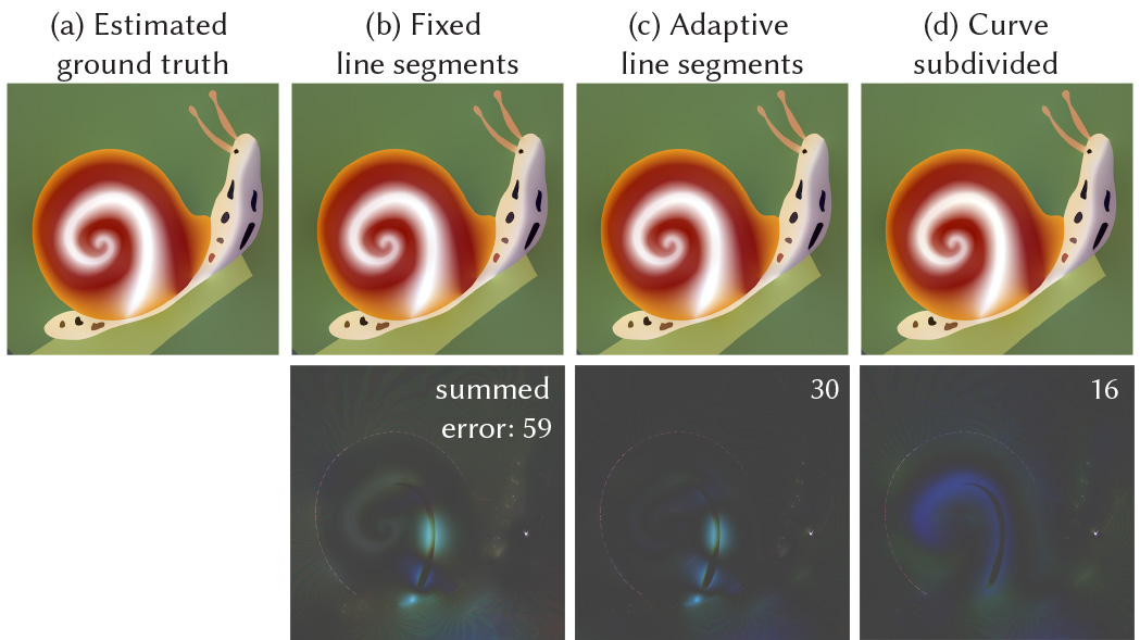
Figure 15. Result comparison of snail example with fixed line segments, adaptive line segments (Sec. 7.2), and adaptive curve subdivision (Sec. 7.1) (top) and its error (bottom).

7.2. Adaptive BEM Line Segments

The number of line segments $s$ at the solving stage can be set to be a small multiple of the number of quadrature points $g$, so if the number of quadrature points on each panel of curve is fixed, then the number of line segments $s$ for the solution stage is fixed as well. In our examples, we set $s=5g$.

The number of line segments $e$ at the evaluation stage, on the other hand, needs to be determined to be just fine enough so that user does not perceive a discretized poly-line, but not so fine as to result in a burdensome computation. Such a choice of $e$ is best determined by the size of the pixel and by the user’s viewport.

Interestingly, it turns out we do not have to make $e$ depend on the pixel size directly. If we set number of the line segments at evaluation stage $e$ to be proportional to the arc-length of the curve plus a constant with the following simple equation,

(57) $$e=(\text{length of curve})/10+s,$$

then the result looks perfectly smooth when zooming in, without requiring an excessive number of calculations. The reason for this is that our adaptive subdivision algorithm for the density, Algorithm 7.1, uses the pixel size as a threshold for subdivision. When the pixel size becomes smaller upon zooming in, the large curves are subdivided, which causes the total number of line segments $s$ on that curve to increase.

Note also that this formula ensures that $e\geq s$, since if $e$ is smaller than $s$, the potential created by the curve will not approximate the potential we solved for in the solution stage.

7.3. Diffusion Curve with Adaptive Subdivision

The overall algorithm for computing a diffusion curve with adaptive subdivision is described by the following algorithm:

Algorithm 7 Diffusion Curve with Adaptive Subdivision

1:Solve for the density at the quadrature points using Algorithm 3 (with a fixed a priori discretization)

2:while  running the adaptive subdivision Algorithm 5 results in subdivided curves do

3:     Update the density with a local re-solve using Algorithm 6

4:Use the FMM to evaluate the single and double-layer potentials at the pixel targets on the viewport domain, choosing the BEM line segments as described in Section 7.2.

Fig. 15 compares the fixed line segments, adaptive line segments, and adaptive curve subdivision (top), showing the resulting error (bottom). Note that the error has been amplified for clear visualization.

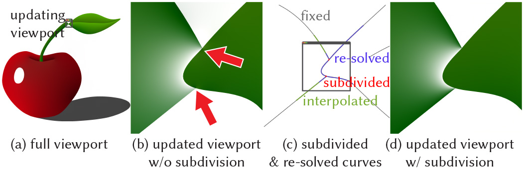
Figure 16. Starting from the full viewport (a), when the user updates the viewport with an extreme zoom-in, artifacts are visible without adaptive subdivision (b). Assigning each curve with a suitable label for efficiency (c) and updating the viewport with adaptive subdivision gives a plausible result (d).

7.4. Updated Viewport

Suppose that the user is exploring the domain with their viewport, so that pixel values need to be re-computed whenever the viewport changes. Re-evaluating pixel values can be done very quickly with Eq. 29, however, whenever the discretization of curves into BEM line segments must change (if the user zooms in, for example), re-solving for the density values will require a heavy re-computation if a BEM-only algorithm is used. This is the moment our hybrid method shines, since we can simply construct interpolated density values for any re-discretized curves using Legendre polynomial interpolation as in Eq. 14. This process of interpolation will work until the viewport domain is zoomed in on such a small region, that the adaptive subdivision process of Algorithm 5 needs further subdivision due to the smaller threshold resulting from the reduced pixel size (see line 2 from Algorithm 5).

To account for a change in viewport, we assign to each curve one of the following three labels: fixed curve, interpolating curve, or re-solving curve (see Figure 16). All curves that are fully outside of the domain of the viewport are labelled as fixed curves. Such curves do not require re-discretization, and can retain their BEM discretization. The curves for which the density must be re-solved according to the algorithm described in Sec. 7.1.4 are labelled as re-solving curves, and include both subdivided curves and neighboring curves. Finally, all of the remaining curves the intersect the viewport are labelled as interpolating-curves, and are re-discretized with smaller BEM line segments using only Legendre polynomial interpolation, with no need for re-solving. Note that, when labeling curves to account for the user’s viewport, the constrained curves of Section 7.1.4 can be either fixed curves or interpolating curves, depending on whether or not they intersect the viewport. Fig. 17 visualizes subdivided and local re-solving curves determined by its viewport domain while a user is zooming-in. Table. 3 is a comparison of computation time with global re-solve and with our local re-solve.

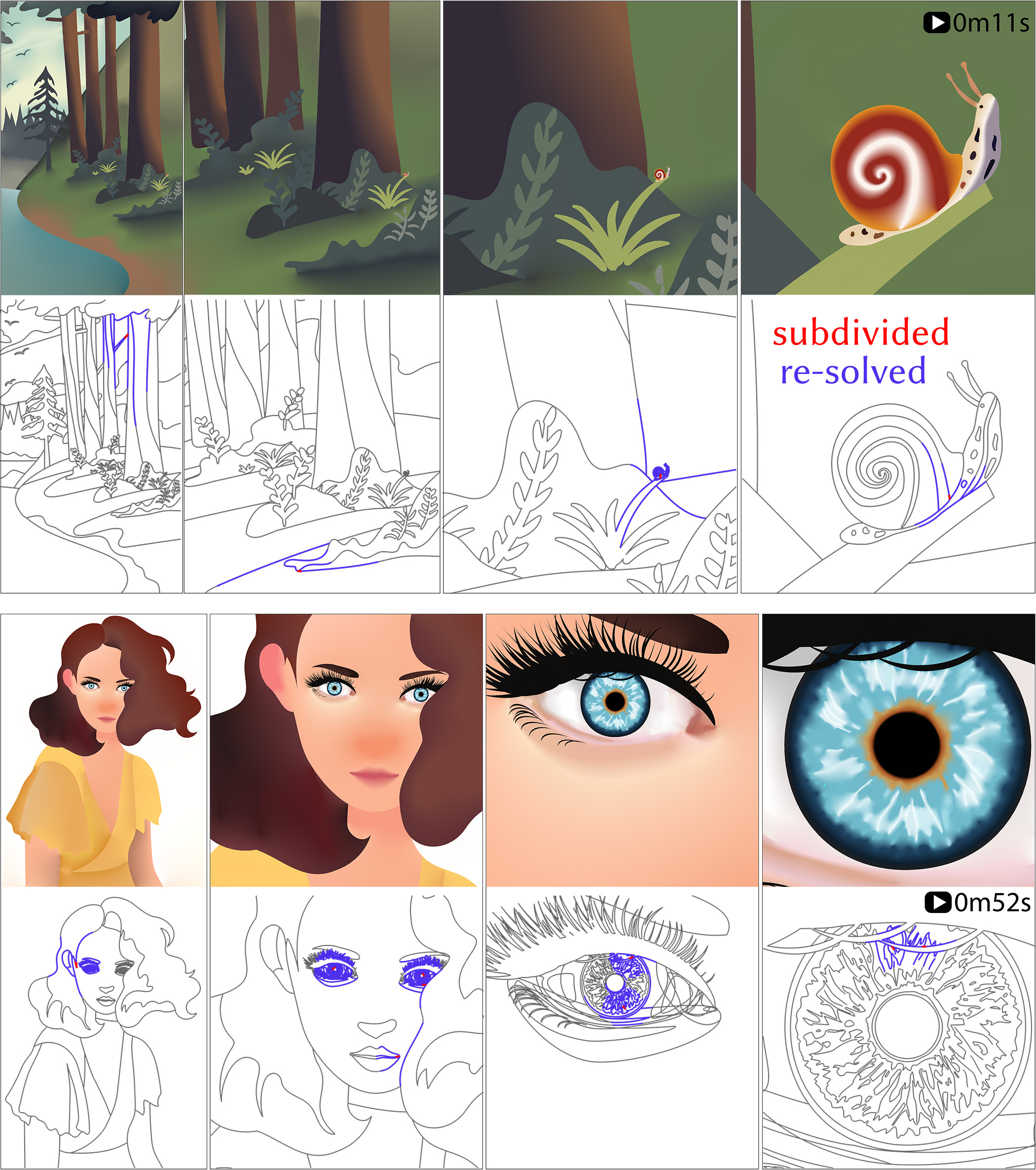
Figure 17. Visualization our of adaptive subdivision procedure while the viewport is zooming in.

Table 3. Computation time comparison between the initial solve of the curve, the global re-solve, and the local re-solve with zoom-in for the example from Fig. 17.

white	Initial	Initial	Global	Local
white	curves	solve	re-solve	re-solve
snail in forest	1493	9.48s	5.35s	0.95s
lady with blue eyes	3126	17.47s	11.29s	1.12s

8. Anti Aliasing

Anti aliasing can be smartly handled using the quadtree structure we built for the FMM. Instead of sampling color values at the mid point of each pixel, we can compute a better estimate of the color values by using area-weighted integration. This can be easily achieved by recursively computing pixel values as weighted sums of pixel values from child cells.

Pixels that are inside cells which are bigger than the pixel size will not benefit from the above strategy. Since we don’t require every pixel to be assigned smaller child cells, the color strategy for such pixels reduces to naive multi sampling. With the key insight that the aliasing happens mostly near boundary curves, we modify the quadtree construction condition so that, if a cell includes any boundary curves, then it will be subdivided until the leaf cell size becomes smaller then the pixel size. This gives a very efficient way of anti aliasing. One limitation of this method is that the total number of pixels is restricted to be $2^{n}$, so that the pixels will always align with the quadtree.

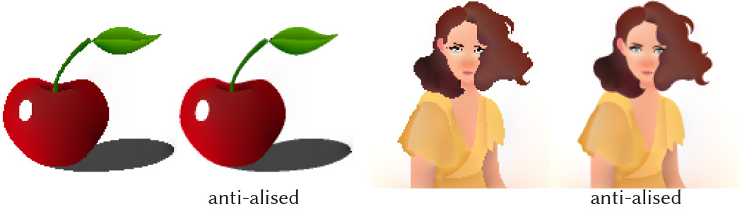
Figure 18. Our method with naive computation of pixel values (left) as well as anti-aliased pixel values (right) on a domain with $128\times 128$ pixels.

9. Results

We demonstrate that our method can accurately compute diffusion curves for a complex set of input curves with drastically differing scales and sizes of details, as demonstrated in Fig. 1. Our algorithm renders the initial diffusion curves by an adaptive method. The diffusion curves then retain their accuracy when the viewport is zoomed into the figure, by an efficient adaptive algorithm that involves re-solving for the density only on a small subset of curves, as shown in Fig. 17. Our adaptive technique is facilitated by our Hybrid Method, which combines the BIEM and BEM, and allows the density to be accurately interpolated on those curves appearing in the viewport which are not re-solved, as shown in Fig. 16.

Our method can also be used to generate high resolution images with existing diffusion curve data from (Orzan et al., 2008), (Jeschke et al., 2011), and (Liu, 2009) as shown in Fig. 19.

We report the computation time in Tables 1,  2, and 3, but note that our implementation is not fully optimized, and has a lot of room for faster computation.

To demonstrate the effect of setting different values of the number of solving BEM segments $s$, Gauss-Legendre nodes $g$, and evaluation BEM segments $e$, we compared the error for different sets of parameters as visualized in Fig. 20. The ground truth here is derived by running BEM with a very large number of BEM segments $e=200$ for each curve. As is clear from the figure, the error gets smaller if we increase the discretization parameters, but the difference is not too large if the numbers are already high enough. Empirically, we found that $s=20,g=4,e=20$ works best in balancing accuracy and performance. Hence, for all the examples in this paper with fixed resolution (in other words, for all of the examples besides Fig.  1 and Fig. 17), we set $s=20,g=4,e=20$, except for the example in Fig. 6, where we set $s=40,g=8,e=40$ for our Hybrid Method.

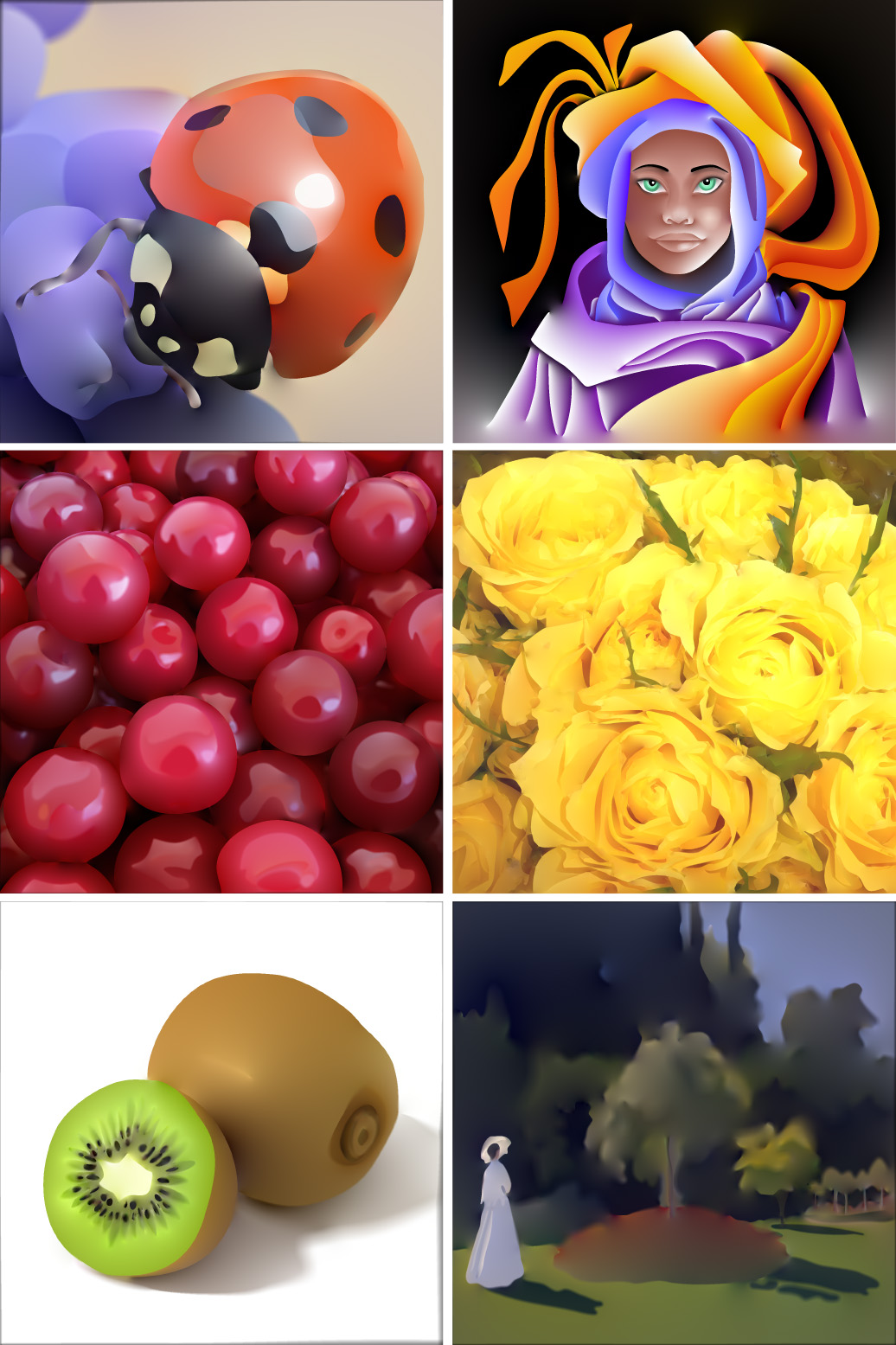
Figure 19. 4K resolution results generated with our method. The blurred scalar field is computed using diffusion curves applied as a postprocessing step. This figure is best viewed on a high-resolution digital screen. Lady bug, person with purple cloak, and yellow roses examples were taken from (Orzan et al., 2008); kiwi and Monet examples were taken from (Jeschke et al., 2011); cherries example was taken from (Sun et al., 2014).

9.1. Implementation

We implemented the main algorithm of our method in C++ with (Jacobson et al., 2018), and additionally used MATLAB and GPTOOLBOX (Jacobson et al., 2021) for development and experimentation. We note that our implementation is not fully optimized, and has a lot of room for improvement. Importantly, our code runs almost entirely on the CPU, and could be accelerated dramatically by an optimized GPU implementation. All the timings were computed on a MacBook Pro laptop with an Intel 2.4GHz Quad-Core i9 Processor and 16GB RAM. Please check the accompanying code to try out the examples.

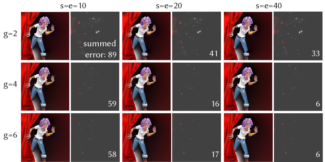
Figure 20. Comparison of different sets of discretization parameters, with highlighted color difference between ground truth, and the summed error indicated in white text. This behind curtain example was taken from (Orzan et al., 2008).

9.2. Comparison with other Methods

The Finite Difference (FD) method (Orzan et al., 2008; Bezerra et al., 2010; Finch et al., 2011) has its strength in its easy parallelization and speed when combined with Multigrid solvers. The main advantage of our method compared to the FD method, is that our method correctly constructs diffusion curves around tiny features, while the FD method flattens down all of its curves to a pixel size, which loses a lot of detailed information. The resulting pixel-level rasterization errors are further amplified by the diffusion process. In Fig. 2 (left), for example, all of the important detail is lost around eye of the woman. Compare this result to Fig. 1 (left). Furthermore, even when no tiny features are present, the rasterization process is not stable to small translations, resulting in strobing artifacts when curves are repositioned.

A solution to this rasterization problem was proposed in (Jeschke et al., 2009). There, rather than rasterizing just the boundary curves, the authors propose rasterizing the entire image by initializing each pixel to the color of the closest curve point. This initial image is then smoothed with a Jacobi-like iteration scheme, in which each pixel is averaged with four axis-aligned pixels lying on a circle, chosen to be sufficiently small so as to not intersect any boundary curves. Since averaging over only axis-aligned pixels instead of the entire circle can create mach-banding-like artifacts, the stencil size is decreased linearly at each step, either immediately, or after performing half of the total number of iterations with the stencil at full size. The iterations on the final stencil are equivalent to classical Jacobi iterations, with boundary constraints enforced by fixed color data near the curves, performed on a good initial guess produced by blending the original image rasterization on the larger stencils. Provided an appropriate shrinking strategy is used, this method can produce a visually excellent diffusion curve image in real-time, with only slight differences with the fully converged image. This method is, however, limited to Dirichlet boundary conditions, and does not take into account curves outside of the image domain. Our method can potentially be extended to Neumann boundary conditions, and handles curves outside of the image domain in a natural way via the FMM.

The Finite Element Method (FEM) (Takayama et al., 2010; Pang et al., 2011; Boyé et al., 2012) is the most widely used method in computer graphics, due to its easy and intuitive implementation with fast Cholesky solvers. However, FEMs suffer from the problem of triangulating the domain. Triangulation of a complex set of curves is itself very difficult problem, and is the subject of current research (Hu et al., 2019). We have attempted to use TriWild (Hu et al., 2019) with the input curves for Fig. 2, but TriWild discarded all of the highly detailed features, and failed if we tried to preserve these features. Even when the triangulation succeeds, the FEM exhibits a bleeding artifact which can be seen in Fig. 3. Using Triangle (Shewchuk, 2005) led to successful triangulation but resulted in more than 10 million triangles given data from Fig. 2. Even with dense triangulations, FEM still shows nonsmooth results near curve endpoints, caused by singularities there. When singularities are present in the PDE solution, both increasing only the polynomial order on elements of fixed size (called p-refinement) or fixing the polynomial order and refining the mesh (called h-refinement) are known to provide only modest improvements in solution accuracy. However, if a carefully chosen combination of mesh refinement and polynomials of varying degree is used, then the FEM can be made to converge exponentially fast (this process is called hp-refinement or the hp-FEM). Such methods, while often effective, can be extremely challenging to implement in a fully automatic fashion (see (Gopal and Trefethen, 2019b)). A heuristic solution for dealing with singularities, proposed by (Boyé et al., 2012), is to linearly blend colors around the vertex of a triangular element lying on a curve endpoint. While visually quite satisfactory, it is worth noting that this approximation is nonetheless very different from the true power-type singularities present at such points. These difficulties, namely the triangulation problem, the bleeding artifact problem, and the singularity problem, are all completely absent in our method. There is no need for triangulation since our method is a boundary-only method, and the bleeding artifact is resolved completely by adaptive subdivision, as seen in Fig. 9.

The pros and cons of the Boundary Element Method (BEM) and Boundary Integral Equation Method (BIEM) are described in Sec. 4. As we discuss in that section, the boundary element method can produce accurate results when many BEM line segments are used, but results in an extremely large linear system to solve. On the other hand, the BIEM has a highly efficient representation of the solution, and results in a small linear system, but creates artifacts when the density is evaluated near the curves. Our Hybrid Method takes the advantages of both, namely, it retains the efficient representation of BIEM while also obtaining the visual quality of BEM, as shown in Fig. 4.

The Walk on Spheres (WoS) method (Sawhney and Crane, 2020) has its strength in its simplicity and its robustness to input data and geometry, but does not generalize efficiently to Neumann boundary conditions, which is a significant limitation, since such boundary conditions are so useful in practice. The two main issues that arise are that WoS can require extremely long walks, and that the sphere sizes near Neumann boundaries become very small, significantly impacting performance. The recently proposed Walk on Stars (WoSt) method (Sawhney et al., 2023) overcomes this second issue by replacing these small spheres with the boundaries of much larger star-shaped domains. Nonetheless, when the boundary is predominantly Neumann (like the boundaries in Fig. 5), WoSt will still can take very long walks, since, like WoS, it must reflect back into the domain from Neumann boundaries and can only terminate at Dirichlet boundaries. This issue can be somewhat ameliorated by caching solution values on the boundary of the domain (Miller et al., 2023), but since the solution values must still be generated by, for example, WoSt, the problem persists. Our method, on the other hand, generalizes to Neumann boundary conditions without difficulty, as shown in Fig 5.

10. Limitations and Future Works

Our proposed method advances diffusion curve representation to a high-accuracy level, accommodating fine multiscale features and allowing precise zooming and panning while maintaining accuracy.

Despite its many desirable features, our method still has some limitations and room for future improvement.

Our Adaptive Strategy was constructed with the assumption that diffusion curves mostly remain static. It will not work efficiently for animated diffusion curves, as it will require large portion of the curve to be re-computed every step.

Our requirement of ensuring accurate computations can become burdensome computationally, because messy or wild curve data will exhibit a lot of intersecting and overlapping curves, which will require heavy adaptive subdivision to resolve. We developed a pre-processing step to deal with ill-posed curves, but it is difficult to distinguish between an intentional ill-posed curve placed by an artist and an unintended ill-posed curve. It will be useful to have a version of our algorithm with softer and less stringent accuracy requirements, which would allow for wilder curve data.

We demonstrate Neumann boundary conditions in the example of Fig. 5. However, our current implementation only supports one-sided Neumann boundary conditions on closed curves. These examples were generated by subdividing a region into disconnected closed subregions. A more general and powerful double-sided Neumann boundary condition is possible, but will require the introduction of a hyper-singular kernel, as described in Sec 2.3 of (Liu, 2009).

Our current implementation is not fully optimized, and does not reach real-time computation speeds. We observed that a GPU-accelerated implementation of brute force computation leads to a speedup of more than 100 times. A GPU-accelerated version of FMM and adaptive re-computation would put on wings on our method and make it truly practical. We leave this extension to our future work.

Appendix A Arc Length Line Segment Integration

Unlike classical BEM, our hybrid method allows for different numbers of BEM line segments at the solution and evaluation stages. In order for us to use different discretizations at each stage, it turns out to be essential that the BEM integration is performed in a way that accounts for the true length of the curve, since the length of a polyline approximation can change if the number of segments changes. Thus, if we naively integrate the line segments, the result will be different if the number of line segments is different. Hence, we employ arc length integration to make sure that different numbers of line segments do not give a different result.

Appendix B Arc Length Parametrization

Unfortunately, there is no closed form solution for the arc length parametrization of a cubic Bézier curve. We employ an iterative method to find the arc length parametrization. Suppose that we have a cubic Bezier curve

(58) $$B:[0,1]\to\mathbb{R}^{2},$$

(59) $$B(t)=(1-t)^{3}C_{0}+3t(1-t)^{2}C_{1}+3t^{2}(1-t)C_{2}+t^{3}C_{3},$$

where $C_{0},C_{1},C_{2},C_{3}\in\mathbb{R}^{2}$ are the control points. Then the cumulative length of the Bezier curve up to some parameter $t=s$ may be written as an integral:

(60) $$L(s)=\int^{s}_{0}\|B^{\prime}(t)\|dt.$$

We apply Newton’s root finding method to find $s$ for a given target arc length $T$ such that $T=L(s)$. Given some guess $s_{0}$, we can improve this guess by the update formula

(61) $$s\leftarrow s_{0}-(L(s)-T)/L^{\prime}(s).$$

However, this requires evaluation of $L(s)$ and $L^{\prime}(s)$. To compute these quantities, we use Gauss-Legendre quadrature to approximate a definite integral over the finite interval $[0,s]$.

Appendix C Singular Green’s Function Integrals

The Green’s function $G(p,q)$ and its normal derivative $F(p,q)$ both have singularities at $p=q$, where the kernel is infinite. To perform accurate BEM integration involving these kernels, it is important to carefully consider how these singularities influence the integrals.

Suppose that $x$ is a target point that approaches the boundary. We divide the boundary $S$ into two parts: $S-S_{\epsilon}$ and $S_{\epsilon}$, where $S_{\epsilon}$ is a small segment with arc length $2\epsilon$ centered around the point to which $x$ will approach.

Let us first consider single layer potential, which involves the integral of the Green’s function $G(p,q)$:

(62) $$\begin{split}\int_{S}G(p,x)\sigma(p)dS(p)=\\ \lim_{\epsilon\to 0}\int_{S-S_{\epsilon}}G(p,x)\sigma(p)dS(p)+\lim_{\begin{subarray}{c}\epsilon\to 0\\ x\to S\end{subarray}}\int_{S_{\epsilon}}G(p,x)\sigma(p)dS(p)\end{split}$$

The limit of the second integral on the right-hand side of Eq. 62 turns out to be

(63) $$\lim_{\begin{subarray}{c}\epsilon\to 0\\ x\to S\end{subarray}}\int_{S_{\epsilon}}G(p,x)\sigma(p)dS(p)=0.$$

Analytic integration of the limit of the first integral on the right-hand side of Eq. 62 over a BEM line segment is described in Appendix D.3.

Let us now consider double layer potential, which involves the integral of the normal derivative of Green’s function, $F(p,q)$:

(64) $$\begin{split}\int_{S}F(p,x)\mu(p)dS(p)=\\ \lim_{\epsilon\to 0}\int_{S-S_{\epsilon}}F(p,x)\mu(p)dS(p)+\lim_{\begin{subarray}{c}\epsilon\to 0\\ x\to S\end{subarray}}\int_{S_{\epsilon}}F(p,x)\mu(p)dS(p)\end{split}$$

The limit of the second integral on the right-hand side of Eq. 64 turns out to be:

(65) $$\lim_{\begin{subarray}{c}\epsilon\to 0\\ x\to S\end{subarray}}\int_{S_{\epsilon}}F(p,x)\mu(p)dS(p)=\pm\frac{1}{2}\mu(x),x\in S.$$

The sign of the one-half $\mu(x)$ depends on which side of the curve the point $x$ approaches.

C.1. Singular Integrals in our Hybrid Method

For standard BEM, the query points are located on the midpoints of each line segment. Thus, for each query point, integration over the singularity happens on the one line segment that is located on the query point, which corresponds to the diagonal entries of $\overline{G}$ and $\overline{F}$.

For our Hybrid Method, the query point can be located at any place along the input curve. If evaluation points (which are also the quadrature points) are positioned near the intersection of two BEM line segments, this situation should be considered as a singular integration for both line segments, and evaluated by invoking Eq. 70 and Eq. 71 in Appendix D.

Appendix D Analytic Integration

In this section, we provide various analytical formulas for evaluating the integrals of the Green’s function kernels $G(p,q)$ and $F(p,q)$ over the line segment $\overline{p_{1}p_{2}}$.

D.1. Integration of Green’s function

The integral of a Green’s function on a line segment can be evaluated analytically as follows:

(66) $$\begin{split}-\int_{S}G(p,q)dS=\int_{S}\frac{\log(|p-q|)}{2\pi}dp\\ =\frac{|a|}{2\pi}\int_{0}^{1}\log(|b+at|)dt=\frac{|a|}{2\pi}\int_{0}^{1}\log(\sqrt{a^{2}t^{2}+2abt+b^{2}})dt,\end{split}$$

where $a=p_{2}-p_{1}$, $b=p_{1}-q$, with $p_{1},p_{2}$ being the endpoints of the line segment. Denoting $a^{2}=\zeta,2ab=\eta,b^{2}=\xi$, we get the following anti-derivative:

(67) $$\begin{split}\frac{|a|}{4\pi}\int_{0}^{1}\log(\zeta t^{2}+\eta t+\xi)dt=\\ \frac{|a|}{4\pi}\left[\log(\zeta t^{2}+\eta t+\xi)(t+\frac{\eta}{\zeta})-\tan^{-1}\left(\frac{2\zeta t+\eta}{\sqrt{4\xi\zeta-\eta^{2}}}\right)\left(\frac{2\zeta+\eta}{\zeta\sqrt{4\xi\zeta-\eta^{2}}}\right)\right]_{0}^{1}=\\ \frac{|a|}{4\pi}\left[\log(\zeta+\eta+\xi)(1+\frac{\eta}{\zeta})-\log(\xi)\frac{\eta}{\zeta}\right]+\\ \frac{|a|}{4\pi}\left[\tan^{-1}\left(\frac{\eta}{\sqrt{4\xi\zeta-\eta^{2}}}\right)-\tan^{-1}\left(\frac{2\zeta+\eta}{\sqrt{4\xi\zeta-\eta^{2}}}\right)\right]\left(\frac{2\zeta+\eta}{\sqrt{4\xi\zeta-\eta^{2}}}\right).\end{split}$$

D.2. Integration of Normal Derivative of Green’s function

The integral of the normal derivative of the Green’s function on a line segment can be evaluated analytically as follows:

(68) $$\begin{split}-\int_{S}F(p,q)dS=\int_{S}\frac{(p-q)\cdot n}{2\pi|p-q|^{2}}dp\\ \frac{1}{2\pi}\int_{0}^{1}\frac{(at+b)\cdot n}{|at+b|^{2}}dt=\frac{b\cdot a^{\perp}}{2\pi}\int_{0}^{1}\frac{1}{a^{2}+2abt+b^{2}}dt,\end{split}$$

where the numerator in the last integral becomes constant because $n=a^{\perp}$. Denoting $2b\cdot a^{\perp}=\nu$, we get the following anti-derivative:

(69) $$\begin{split}\frac{\nu}{2\pi}\int_{0}^{1}\frac{1}{\zeta t^{2}+\eta t+\xi}dt\\ \frac{\nu}{2\pi}\left[\tan^{-1}\left(\frac{2\zeta t+\eta}{\sqrt{4\xi\zeta-\eta^{2}}}\right)\left(\frac{\nu}{\sqrt{4\xi\zeta-\eta^{2}}}\right)\right]_{0}^{1}=\\ \frac{\nu}{2\pi}\left[\tan^{-1}\left(\frac{2\zeta+\eta}{\sqrt{4\xi\zeta-\eta^{2}}}\right)\tan^{-1}\left(\frac{\eta}{\sqrt{4\xi\zeta-\eta^{2}}}\right)\right]\left(\frac{\nu}{\sqrt{4\xi\zeta-\eta^{2}}}\right).\end{split}$$

D.3. Singular Integration of Green’s function

Singular integration happens when $q$ lies on the line segment $\overline{p_{1}p_{2}}$. Letting $b=at^{*}$, the integral can be expressed simply as:

(70) $$\begin{split}\frac{|a|}{2\pi}\int_{0}^{1}\log(|a(t-t^{*})|)dt=\\ \frac{|a|}{2\pi}\lim_{\epsilon\to 0}\left(\int_{0}^{t^{*}-\epsilon}\log(|a(t-t^{*})|)dt+\int_{t^{*}+\epsilon}^{1}\log(|a(t-t^{*})|)dt\right)=\\ \frac{|a|}{4\pi}\lim_{\epsilon\to 0}\left[-2t+(t-t^{*})\log(a^{2}(t-t^{*})^{2})\right]_{0}^{t^{*}-\epsilon}+\\ \frac{|a|}{4\pi}\lim_{\epsilon\to 0}\left[-2t+(t-t^{*})\log(a^{2}(t-t^{*})^{2})\right]_{t^{*}+\epsilon}^{1}=\\ \frac{1}{4\pi}\left(2|a|-|a|t^{*}\log(|a|^{2}{t^{*}}^{2})+(|a|t^{*}-|a|)\log(|a|^{2}(1-t^{*})^{2})\right)=\\ \frac{1}{2\pi}(s-e_{1}\log e_{1}-e_{2}\log e_{2}),\end{split}$$

where $s=|a|$, $e_{1}=\overline{qp_{1}}=|a|t^{*}$, and $e_{2}=\overline{qp_{2}}=|a|(1-t^{*})$.

D.4. Singular Integration of Normal Derivative of Green’s function

Similar to the above approach, we can express the singular integral as:

(71) $$\begin{split}\frac{|a|}{2\pi}\int_{0}^{1}\frac{a(t-t^{*})\cdot n}{|a(t-t^{*})|^{2}}dt.\end{split}$$

The above equation becomes $0$ since $(t-t^{*})\cdot n=0$.

Appendix E Fast Multiple Method

Consider the evaluation of the BEM integrals in Eq. 8 over $m$ diffusion curves, for a total of $N=ms$ BEM line segments. Directly evaluating the BEM integrals in Eq. 8 or Eq. 10 at $M$ target points requires $\mathcal{O}(NM)$ operations. Greengard and Roklin (Greengard and Rokhlin, 1987) demonstrated that the task could be done in $\mathcal{O}(N+M)$ operations in finite precision by introducing the Fast Multipole Method (FMM), which is asymptotically even better than the $\mathcal{O}(N\log(N)+M\log(M))$ operations required by the Barnes-Hut algorithm (Barnes and Hut, 1986; Pfalzner and Gibbon, 1997). In this section, we provide an introduction to the FMM for the complex-valued kernel $G(p,q)=-\frac{1}{2\pi}\log(q-p)$, whose real part is the Green’s function defined in Eq. 2, where $p$ and $q$ are treated as points in the complex plane.

E.1. Multipole expansion

The key idea behind the Fast Multipole Method is the observation that, if a potential is induced by a source involving a Green’s function, then the potential away from the source can be approximated to high accuracy by a finite sum involving certain basis functions, where the number of terms involved in the sum is independent of the complexity of the source distribution. These sums approximating the induced potential are called expansions.

E.1.1. Outgoing expansion

Suppose we have the source curve $S_{\beta}$ contained in a cell $\Omega_{\beta}$, and that we have a query point located far from this cell, separated by at least one cell width (see inset). In this case, we say that a query point is well-separated from cell $\Omega_{\beta}$. The outgoing expansion is the expansion which represents the potential induced by this source curve, at all well-separated target points. The word outgoing reflects the fact that this expansion is directed outwards from the source curve, and is valid for all target points far away.

Letting $c_{\beta}$ be the point at the center of the cell $\Omega_{\beta}$, we observe that the Green’s function kernel $G(p,q)$ can be written as

(72) $$G(p,q)=-\frac{1}{2\pi}\log(q-p)$$

(73) $$=-\frac{1}{2\pi}[\log(q-c_{\beta})+\log(1-\frac{p-c_{\beta}}{q-c_{\beta}})].$$

Using the Taylor series expansion for $\log$,

(74) $$\log(1-z)=-\sum_{k=1}^{\infty}\frac{z^{k}}{k}\quad\text{for}\quad|z|<1,$$

we see that

(75) $$G(p,q)=-\frac{1}{2\pi}[\log(q-c_{\beta})-\sum_{k=1}^{\infty}\frac{1}{k}\bigl{(}\frac{p-c_{\beta}}{q-c_{\beta}}\bigr{)}^{k}].$$

Since $p$ is in $\Omega_{\beta}$, and $q$ is at least one cell width away, it’s not difficult to show that that ${\lvert p-c_{\beta}\rvert}/{\lvert q-c_{\beta}\rvert}\leq\sqrt{2}/3<1$. Therefore, the terms in the infinite sum above decay exponentially fast at the rate $(\sqrt{2}/3)^{k}$. This means that we can truncate the series to only $K$ terms, where $K$ is independent of the source curve $S_{\beta}$ and the query point $q$, and depends only on the desired accuracy.

Applying this observation to the Green’s function kernel, we have

(76) $$G(p,q)=\frac{1}{2\pi}\sum_{k=0}^{K}O_{k}(q-c_{\beta})I_{k}(p-c_{\beta}),$$

where

(77) $$I_{k}(p-c_{\beta})=\frac{(p-c_{\beta})^{k}}{k!}\quad\text{for}\quad k\geq 0,$$

and

(78) $$O_{k}(q-c_{\beta})=\frac{(k-1)!}{(q-c_{\beta})^{k}}\quad\text{for}\quad k\geq 1\quad\text{and}\quad O_{0}(q-c_{\beta})=-\log(q-c_{\beta}).$$

Thus, to evaluate the potential $u^{q}$ created by the density $\sigma$ on the curve $S_{\beta}$,

(79) $$u^{q}=\underbrace{\int_{S_{\beta}}G(p,q)\sigma(p)dS(p),}_{\textrm{target-from-source}}$$

all that is needed are the coefficients $\hat{\bm{\sigma}}^{\beta}$,

(80) $$\hat{\bm{\sigma}}^{\beta}_{k}=\underbrace{\int_{S_{\beta}}I_{k}(p-c_{\beta})\sigma(p)dS(p),}_{\textrm{outgoing-from-source}}$$

for $k=0,1,\ldots,K$, from which the potential ${u}^{q}$ is evaluted by the formula

(81) $$u^{q}=\underbrace{\frac{1}{2\pi}\sum_{k=0}^{K}O_{k}(q-c_{\beta})\hat{\bm{\sigma}}^{\beta}_{k}.}_{\textrm{target-from-outgoing}}$$

Suppose that the integrals in the target-from-source and outgoing-from-source formulas require $M$ degrees of freedom to evaluate. To create the outgoing expansion, we expend $KM=\mathcal{O}(M)$ operations to evaluate the outgoing-from-source formulas. If we then evaluate the potential at $N$ well-separated target points $q$ using the target-from-outgoing formula, the cost will be only $KN=\mathcal{O}(N)$. This is much faster than evaluating the potential directly using the target-from-source formula, since that would require $MN$ operations.

E.1.2. Incoming expansion

There is another alternative way of accelerating the evaluation of the potential induced by an integral of a Green’s function over a source curve. Suppose that we have a query point $q$ contained in a cell $\Omega_{\alpha}$, and that there is a source curve $S$ that is separated from $\Omega_{\alpha}$ by at least on cell width (see inset). We can construct an incoming expansion on $\Omega_{\alpha}$ for the potential created by this source curve, which is directed inwards, in the sense that it is valid only for target points $q$ inside $\Omega_{\alpha}$.

We can express the Green’s function kernel as:

(82) $$G(p,q)=\frac{1}{2\pi}\sum_{k=0}^{K}O_{k}(p-c_{\alpha})I_{k}(q-c_{\alpha}),$$

where $q$ is in $\Omega_{\alpha}$ and $p$ is at least one cell-width away. Thus, to evaluate the potential $u^{q}$ generated by the density $\sigma$ on the curve $S$ (see Eq. 79), all that is needed are the coefficients $\hat{\mathbf{u}}^{\alpha}$,

(83) $$\hat{\mathbf{u}}^{\alpha}_{k}=\underbrace{\int_{S}O_{k}(p-c_{\alpha})\sigma(p)dS(p)}_{\textrm{incoming-from-source}},$$

for $k=0,1,\ldots,K$, from which the potential $u^{q}$ is evaluated by the formula

(84) $$u^{q}=\underbrace{\frac{1}{2\pi}\sum_{k=0}^{K}I_{k}(q-c_{\alpha})\hat{\mathbf{u}}^{\alpha}_{k}.}_{\textrm{target-from-incoming}}$$

Suppose, like before, that the integrals in the target-from-source and incoming-from-source formulas require $M$ degrees of freedom to evaluate. To create an incoming expansion, we expend $KM=\mathcal{O}(M)$ operations to evaluate the incoming-from-source formulas. If we then evaluate the potential at $N$ target points $q$ inside $\Omega_{\alpha}$ using the target-from-incoming formula, then the cost will be only $KN=\mathcal{O}(N)$. This is much faster than evaluating the potential directly using the target-from-source formula, since that would require $MN$ operations.

E.1.3. Incoming-from-Outgoing

Suppose now that we have $N$ query points contained in a cell $\Omega_{\alpha}$ with center $c_{\alpha}$, and that there are $m$ cells containing source curves, all well-separated from the cell $\Omega_{\alpha}$. If we construct outgoing-from-source expansions for each source cell, then the cost of evaluating the potential using the target-from-outgoing expansions will be $mK$ for each query point $q$ in $\Omega_{\alpha}$, for a total evaluation cost of $NmK=\mathcal{O}(Nm)$. However, if we could construct a single incoming expansion on $\Omega_{\alpha}$ from all $m$ outgoing expansions, then the cost of evaluating the potential using the target-from-incoming expansion would be only $K$ for each query point $q$ in $\Omega_{\alpha}$, for a total evaluation cost of $NK=\mathcal{O}(N)$. We can construct an incoming expansion from an outgoing expansion, as follows.

Suppose that $\hat{\bm{\sigma}}^{\beta}$ is an outgoing expansion for the cell $\Omega_{\beta}$, where $\Omega_{\beta}$ is well-separated from $\Omega_{\alpha}$. Recall the target-from-outgoing formula

(85) $$u^{q}=\frac{1}{2\pi}\sum_{k=0}^{K}O_{k}(q-c_{\beta})\hat{\bm{\sigma}}^{\beta}_{k}$$

$$=\frac{1}{2\pi}\sum_{k=0}^{K}O_{k}[(q-c_{\alpha})+(c_{\alpha}-c_{\beta})]\hat{\bm{\sigma}}^{\beta}_{k},$$

where $u^{q}$ is the potential at the query point $q$ in $\Omega_{\alpha}$. If there are two terms inside the $O_{k}$ function, we can separate them using the formula

(86) $$O_{k}(z_{1}+z_{2})=\sum_{l=0}^{K}(-1)^{l}O_{k+l}(z_{1})I_{l}(z_{2}).$$

Applying Eq. 86 and exchanging the order of summation, we have

(87) $$u^{q}=\sum_{k=0}^{K}I_{k}(q-c_{\alpha})\hat{\mathbf{u}}^{\alpha}_{k},$$

where

(88) $$\hat{\mathbf{u}}^{\alpha}_{l}=\underbrace{(-1)^{l}\sum_{k=0}^{K}O_{l+k}(c_{\alpha}-c_{\beta})\hat{\bm{\sigma}}^{\beta}_{k}.}_{\textrm{incoming-from-outgoing}}$$

Thus, we can turn an outgoing expansion into an incoming expansion with $K^{2}$ operations. The cost of turning all outgoing expansions into incoming expansions in the previous example is thus $K^{2}m=\mathcal{O}(m)$. Recalling that the cost of evaluating the incoming expansion is $\mathcal{O}(N)$, we have a total cost of $\mathcal{O}(m+N)$, which is much better than the $\mathcal{O}(Nm)$ cost of evaluating all of the outgoing expansions naively.

E.2. A Single-level Method

Suppose that the computational domain contains a collection of diffusion curves, and that all of their integrals can be discretized using a total of $M$ degrees of freedom. Suppose further that we would like to evaluate the potential induced by these curves at $N$ points. Suppose finally that the computational domain containing all curves and evaluation points is divided into $m$ boxes or cells. The three expansions described in the previous section can be used to accelerate the evaluation of the potential.

First, we define the following relations betweens cells in our computational domain.

• The neighbor list $\mathcal{L}^{\textrm{nei}}_{\tau}$ of the cell $\Omega_{\tau}$ (dark blue cell inset) is the set of all boxes that directly touch $\Omega_{\tau}$ (light blue cells inset).

• The well-separated list $\mathcal{L}^{\textrm{sep}}_{\tau}$ of the cell $\Omega_{\tau}$ is the set of all boxes that do not touch $\Omega_{\tau}$ (orange cells inset).

The algorithm proceeds as follows. An outgoing expansion is constructed for every box using the outgoing-from-source formula Eq. 80. Next, for each box $\Omega_{\tau}$, all outgoing expansions in the well-separated list $\mathcal{L}^{\textrm{sep}}_{\tau}$ are turned into incoming expansions using the incoming-from-outgoing formula Eq. 88. Finally, for each box $\Omega_{\tau}$, all incoming expansions are evaluated at the target points using the target-from-incoming formula Eq. 84, and then added to the potentials produced by all sources in the neighbor list $\mathcal{L}^{\textrm{nei}}_{\tau}$ using the target-from-source formula Eq. 79. If $m$ is chosen to be $m=(NM)^{\frac{1}{3}}$, then we show in Appendix F that the overall cost is $\mathcal{O}((NM)^{\frac{2}{3}})$, which is substantially better than the $\mathcal{O}(NM)$ cost of computing the potential at all $N$ points naively.

E.3. Moving Between Levels in the Fast Multipole Method

The single-level method described in the previous section can be further improved by defining a multi-level hierarchy of boxes on the computational domain, and taking advantage of the fact that the number of terms $K$ in the incoming and outgoing expansions stays constant across levels in this hierarchy. The resulting method is called the Fast Multipole Method (FMM).

The primary geometric data structure used by the FMM is the quadtree, which is constructed recursively by starting from a single cell containing the whole domain, and splitting each cell into 4 equal-sized smaller cells until each cell contains a small number of degrees of freedom, or the algorithm reaches a prescribed maximum depth.

E.3.1. Relations between Cells

To describe the multi-level scheme, we must first introduce several additional relations between cells in the hierarchy, besides the neighbor list $\mathcal{L}^{\textrm{nei}}_{\tau}$ and well-separated list $\mathcal{L}^{\textrm{sep}}_{\tau}$ of the box $\Omega_{\tau}$, introduced in the previous section.

• The parent of a cell $\Omega_{\tau}$ is the cell on the next coarsest level that contains $\Omega_{\tau}$.

• The child list of a cell $\Omega_{\tau}$ is the set $\mathcal{L}^{\textrm{child}}_{\tau}$ containing the 4 cells whose parent is $\Omega_{\tau}$.

• The leaf cells are the cells that don’t have any children.

• The interaction list of a cell $\Omega_{\tau}$ is the set $\mathcal{L}^{\textrm{int}}_{\tau}$ containing all cells $\Omega_{\sigma}$ such that: 1) $\Omega_{\tau}$ and $\Omega_{\sigma}$ are on the same level and well-separated to each other, 2) the parents of $\Omega_{\tau}$ and $\Omega_{\sigma}$ is not well-separated

Note that the interaction list is a subset of the well-separated list defined in the previous section, since two boxes on the same level cannot touch without their parents also touching.

To proceed, we need a way of moving information between levels in the multi-level hierarchy, in the form of outgoing and incoming expansions. The formulas relating expansions between different levels of the quadtree are also called translation operators.

E.3.2. Outgoing-from-Outgoing

Consider a parent cell $\Omega_{\beta^{{}^{\prime}}}$ containing 4 child cells. Suppose that $\Omega_{\beta}$ is a child of $\Omega_{\beta^{\prime}}$, and that we have already computed the outgoing expansion $\hat{\bm{\sigma}}^{\beta}$ on $\Omega_{\beta}$. Then, we can transfer the outgoing expansions from the child to the parent, as follows. First, recall the target-from-outgoing formula

(89) $$u^{q}=\frac{1}{2\pi}\sum_{k=0}^{K}O_{k}(q-c_{\beta})\hat{\bm{\sigma}}^{\beta}_{k}$$

$$=\frac{1}{2\pi}\sum_{k=0}^{K}O_{k}[(q-c_{\beta^{\prime}})+(c_{\beta^{\prime}}-c_{\beta})]\hat{\bm{\sigma}}^{\beta}_{k}.$$

Applying Eq. 86 and exchanging the order of summation, we have

(90) $$u^{q}=\frac{1}{2\pi}\sum_{k=0}^{K}O_{k}(q-c_{\beta^{\prime}})\hat{\bm{\sigma}}^{\beta^{\prime}}_{k}$$

where

(91) $$\hat{\bm{\sigma}}^{\beta^{\prime}}_{k}=\underbrace{\sum_{l=0}^{k}I_{k-l}(c_{\beta}-c_{\beta^{{}^{\prime}}})\hat{\bm{\sigma}}^{\beta}_{l}.}_{\textrm{outgoing-from-outgoing}}$$

This outgoing-from-outgoing formula transfers an outgoing expansion from the child cell $\Omega_{\beta}$ to the parent cell $\Omega_{\beta^{\prime}}$

E.3.3. Incoming-from-Incoming

Likewise, an incoming expansion can be transferred from a parent cell to a child cell. Suppose that $\Omega_{\alpha}$ is a child of $\Omega_{\alpha^{\prime}}$, and that we have already computed the incoming expansion of $\hat{\bm{u}}^{\alpha^{\prime}}$ of $\Omega_{\alpha^{\prime}}$. We can transfer the incoming expansion from the parent to the child, as follows. Recall the target-from-incoming formula

(92) $$u^{q}=\frac{1}{2\pi}\sum_{l=0}^{K}I_{l}(q-c_{\alpha^{\prime}})\hat{\bm{u}}^{\alpha^{\prime}}_{l}$$

$$=\frac{1}{2\pi}\sum_{l=0}^{K}I_{l}[(q-c_{\alpha})+(c_{\alpha}-c_{\alpha^{\prime}})]\hat{\bm{u}}^{\alpha^{\prime}}_{l}.$$

Similarly to Eq. 86, when there are two terms inside the $I_{l}$ function, we can separate them:

(93) $$I_{l}(z_{1}+z_{2})=\sum_{k=0}^{l}I_{l-k}(z_{1})I_{k}(z_{2}).$$

Applying Eq. 93, we obtain the following equation:

(94) $$u^{q}=\frac{1}{2\pi}\sum_{l=0}^{K}I_{l}(q-c_{\alpha})\hat{\bm{u}}^{\alpha}_{l},$$

where,

(95) $$\hat{\bm{u}}^{\alpha}_{l}=\underbrace{\sum_{k=l}^{K}I_{k-l}(c_{\alpha}-c_{\alpha^{\prime}})\hat{\bm{u}}_{k}^{\alpha^{\prime}}}_{\textrm{incoming-from-incoming}}.$$

This incoming-from-incoming formula transfers an incoming expansion from the parent cell $\Omega_{\alpha^{\prime}}$ to its child cell $\Omega_{\alpha}$.

E.4. The Fast Multipole Method on a Uniform Quadtree

A uniform quadtree is a quadtree in which all leaf cells occur at the same level of the tree. On a uniform quadtree, the Fast Multipole Method proceeds as follows. Suppose that the computational domain contains a collection of diffusion curves which can be discretized using $M$ degrees of freedom. Suppose further that we would like to evaluate the potential induced by these curves at $N$ points. Suppose finally that we construct our quadtree by subdividing until fewer than $b$ degrees of freedom are contained in each leaf box. To proceed, first, all outgoing expansions are formed on all of the leaf cells on the lowest level in the hierarchy using the outgoing-from-source formula Eq. 80. Then, outgoing expansions are formed on coarser grids, going from finest to coarsest, by merging outgoing expansions using the outgoing-from-outgoing formula Eq. 91.

Once all outgoing expansions on all levels have been constructed, incoming expansions are formed, going from the coarsest grid to the finest. In particular, incoming expansions are first formed on all cells on the coarsest grid by applying the incoming-from-outgoing formula Eq. 88 to all outgoing expansions in the well-separated list $\mathcal{L}^{\text{sep}}_{\tau}$ of each cell $\Omega_{\tau}$. Then, on each successive level, the incoming expansion of each cell $\Omega_{\tau}$ is formed by first transferring the incoming expansion from the parent cell $\Omega_{\tau^{\prime}}$ using the incoming-from-incoming formula Eq. 95, and then by turning all outgoing expansions in the interaction list $\mathcal{L}_{\tau}^{\text{int}}$ into incoming expansions, using the incoming-from-outgoing formula Eq. 88.

Finally, for each cell $\Omega_{\tau}$, the incoming expansions are evaluated at the target points using the target-from-incoming formula Eq. 84, and then these values are added to the potentials from the sources in the neighbor list $\mathcal{L}_{\tau}^{\text{nei}}$, which are evaluated directly using the target-from-source formula Eq. 79.

In Appendix G, we show that if we choose $b=K$, then the total cost is $\mathcal{O}(KM+KN)$, so it is linear in both the number of degrees of freedom in the sources $M$ and the number of targets $N$.

E.5. Extension to a Non-uniform Quadtree

If we allow leaf cells to occur on different levels of the quadtree, then the quadtree is called non-uniform. For such a quadtree, the method described in Section E.4 can fail, since there may be cells which end up unaccounted for.

E.5.1. Relations between Cells

We will need to introduce two more relations between cells, in addition to the ones introduced already in Section E.2 and E.3.1.

• The smaller separated list $\mathcal{L}^{\text{small}}_{\alpha}$ of the leaf cell $\Omega_{\alpha}$ is the set of cells $\Omega_{\beta}$ that are smaller than the cell $\Omega_{\alpha}$, such that $\Omega_{\alpha}$ is in the well-separated list $\mathcal{L}^{\text{sep}}_{\beta}$ of $\Omega_{\beta}$, and $\Omega_{\alpha}$ is not in the well-separated list $\mathcal{L}^{\text{sep}}_{\beta^{\prime}}$ of the parent cell $\Omega_{\beta^{\prime}}$ of $\Omega_{\beta}$ (see Fig. 22 (d)).

• The bigger separated list $\mathcal{L}^{\text{big}}_{\alpha}$ is the dual of the smaller separated list, in the sense that a cell $\Omega_{\beta}$ is in $\mathcal{L}^{\text{big}}_{\alpha}$ if and only if $\Omega_{\alpha}$ is in $\mathcal{L}^{\text{small}}_{\beta}$. It is not too hard to show that the bigger separated list $\mathcal{L}^{\text{big}}_{\alpha}$ of the cell $\Omega_{\alpha}$ is the set of leaf cells $\Omega_{\beta}$ that are larger than the cell $\Omega_{\alpha}$, such that that $\Omega_{\beta}$ is in the well-separated list $\mathcal{L}^{\text{sep}}_{\alpha}$ of $\Omega_{\alpha}$, and $\Omega_{\beta}$ is not in the well-separated list $\mathcal{L}^{\text{sep}}_{\alpha^{\prime}}$ of the parent cell $\Omega_{\alpha^{\prime}}$ of $\Omega_{\alpha}$ (see Fig. 22 (e)).

In the FMM literature, the lists $\mathcal{L}^{\text{small}}_{\tau}$ and $\mathcal{L}^{\text{big}}_{\tau}$ are sometimes called list 3 and list 4, and denoted by $\mathcal{L}^{\text{(3)}}_{\tau}$ and $\mathcal{L}^{\text{(4)}}_{\tau}$, respectively (Martinsson, 2019).

It is not difficult to show that the interactions between any two leaf cells on a non-uniform quadtree are accounted for by the outgoing-from-source to incoming-from-outgoing to target-from-incoming calculation, if and only if those two leaf cells are in each other’s separated lists (see Fig. 21). If two leaf cells $\Omega_{\alpha}$ and $\Omega_{\beta}$ are not mutually well-separated, then one of the following three cases must occur: $\Omega_{\alpha}$ and $\Omega_{\beta}$ are touching; $\Omega_{\beta}$ (or one of its parent cells on a sufficiently high level) is in the smaller separated list of $\Omega_{\alpha}$; or $\Omega_{\beta}$ is in the bigger separated list of $\Omega_{\alpha}$ (or one of its parent cells on a sufficiently high level).

When two cells are not mutually well-separated and are not touching, it is necessary to skip part of incoming-from-outgoing and directly proceed target-from-outgoing or incoming-from-source

E.5.2. Target-from-Outgoing

Suppose that $\Omega_{\beta}$ is in the smaller separated list $\mathcal{L}_{\alpha}^{\text{small}}$ of the leaf cell $\Omega_{\alpha}$. In this case, we cannot use the incoming expansion on $\Omega_{\beta}$, but the outgoing expansion on $\Omega_{\alpha}$ is still valid. Hence, we use the target-from-outgoing formula Eq. 81, skipping the incoming expansion step (see above Figure and Fig. 21).

E.5.3. Incoming-from-Source

Suppose that the leaf cell $\Omega_{\beta}$ is in the bigger separated list $\mathcal{L}_{\alpha}^{\text{big}}$ of $\Omega_{\alpha}$. In this case, we cannot use the outgoing expansion on $\Omega_{\beta}$, but the incoming expansion on $\Omega_{\alpha}$ is still valid. Hence, we use the incoming-from-source formula Eq. 83, skipping the outgoing expansion step (see above Figure and Fig. 21).

E.6. Interaction between Cells

Through Sec. E.1 to Sec. E.5, we have established various routes of integration depending on the cell relations. In summary, there are 4 paths of integration between source and target.

Fig. 21 visualizes each path of integration between cells.

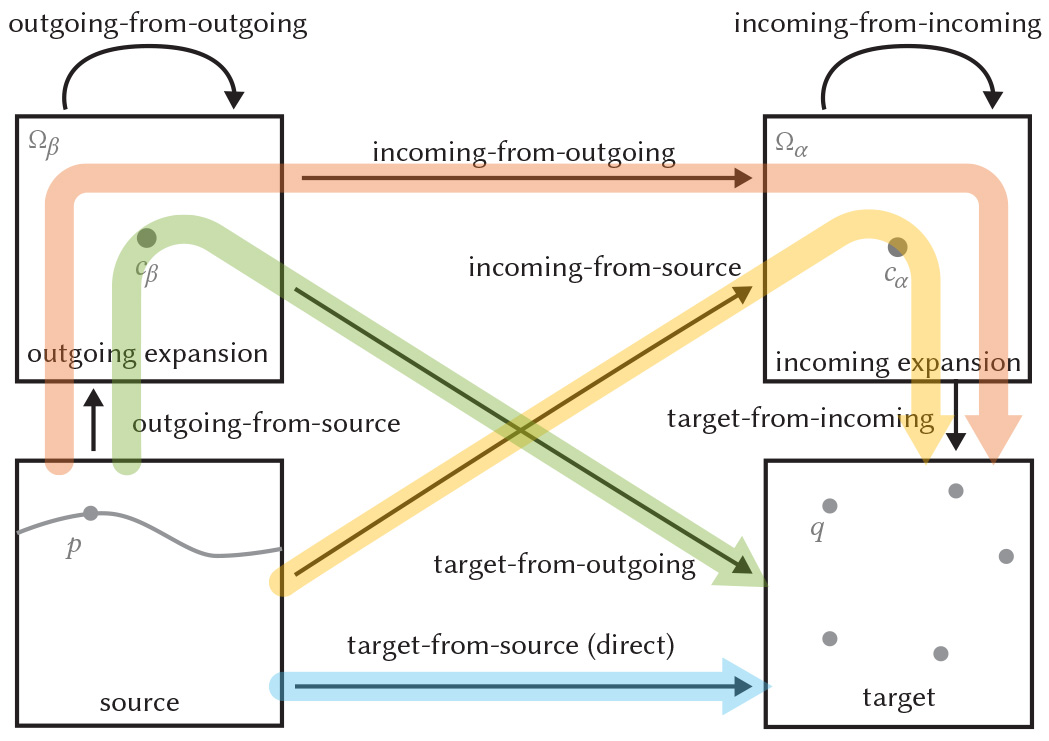
Figure 21. Diagram describing the flow of computations in the FMM by various routes.

E.7. The Fast Multipole Method

Suppose that the computational domain contains a collection of diffusion curves which can be discretized using $M$ degrees of freedom. Suppose further that we would like to evaluate the potential induced by these curves at $N$ points. Suppose finally that we construct our quadtree by subdividing until fewer than $b$ degrees of freedom are contained in each leaf box, allowing leaf boxes of different sizes. The Fast Multipole Method, on a nonuniform quadtree, proceeds as follows. First, all outgoing expansions are formed on all of the leaf cells on the lowest level in the hierarchy using the outgoing-from-source formula Eq. 80. Next, the outgoing expansions are formed on coarser grids, going from finest to coarsest, by merging outgoing expansions using the outgoing-from-outgoing formula Eq. 91.

Once all outgoing expansions on all levels are formed, incoming expansions are constructed, going from the coarsest grid to the finest. In particular, incoming expansions are first formed on all cells on the coarsest grid by applying the incoming-from-outgoing formula Eq. 88 to all outgoing expansions in the well-separated list $\mathcal{L}^{\text{sep}}_{\alpha}$ of each cell $\Omega_{\alpha}$. Then, on each successive level, the incoming expansion of each cell $\Omega_{\alpha}$ is formed from the incoming expansion of the parent cell $\Omega_{\alpha^{\prime}}$, by transferring the expansion to $\Omega_{\alpha}$ using the incoming-from-incoming formula Eq. 95. These incoming expansions are added to the incoming expansions constructed from all of the cells in the interaction list $\mathcal{L}^{\text{int}}_{\alpha}$ using the incoming-from-outgoing formula Eq. 88, and from all cells in the bigger separated list $\mathcal{L}^{\text{big}}_{\alpha}$ using the incoming-from-source formula Eq. 83.

For each leaf cell $\Omega_{\alpha}$, the potential is evaluated at the target points using the target-from-incoming formula Eq. 84. This potential is then added to the potential produced by every cell $\Omega_{\beta}$ is the smaller separated list $\mathcal{L}^{\text{small}}_{\alpha}$ using the target-from-outgoing formula Eq. 81. Finally, these values are added to the potentials from the source cells in the neighbor list $\mathcal{L}_{\alpha}^{\text{nei}}$, which are evaluated directly using the target-from-source formula Eq. 79.

The overall algorithm in pseudo code is described in Table 8 and the cell relations with an example set of input curves is visualized in Fig. 22. Recalling that the incoming and outgoing expansions contain only $K$ terms, if we set $b=K$, then we have, by an essentially identical argument to the one provided in Appendix G, that the total cost is $\mathcal{O}(KM+KN)$, so it is linear in both the number of degrees of freedom in the source curves $M$, and the number of targets $N$.

Algorithm 8 Fast Multipole Method

Inputs: source curves $S$, density values $\sigma$, target points $q$

Outputs: target values $u^{q}$

1:loop  over every leaf cell $\Omega_{\beta}$:

2:     $\hat{\bm{\sigma}}^{\beta}=\text{outgoing-from-source}(S_{\beta},\sigma)$

3:upward  (from finest to coarsest level):

4:     loop  over every cell $\Omega_{\beta^{\prime}}$ in level:

5:         Initialize $\hat{\bm{\sigma}}^{\beta^{\prime}}=\bm{0}$

6:         loop  over every child cell $\Omega_{\beta}\in\mathcal{L}_{\beta^{\prime}}^{\text{child}}$:

7:              $\hat{\bm{\sigma}}^{\beta^{\prime}}=\hat{\bm{\sigma}}^{\beta^{\prime}}+\text{outgoing-from-outgoing}(\hat{\bm{\sigma}}^{\beta})$               

8:downward  (from coarsest to finest level):

9:     loop  over every cell $\Omega_{\alpha}$ in level:

10:         Initialize $\hat{\bm{u}}^{\alpha}=\bm{0}$

11:         loop  over every cell $\Omega_{\beta}$ in interaction list $\mathcal{L}_{\alpha}^{\text{int}}$ (or separated list $\mathcal{L}_{\alpha}^{\text{sep}}$ when at the top level):

12:              $\hat{\bm{u}}^{\alpha}=\hat{\bm{u}}^{\alpha}+\text{incoming-from-outgoing}(\hat{\bm{\sigma}}_{\beta})$          

13:         loop  over every cell $\Omega_{\beta}$ in bigger separated list $\mathcal{L}_{\alpha}^{\text{big}}$:

14:              $\hat{\bm{u}}^{\alpha}=\hat{\bm{u}}^{\alpha}+\text{incoming-from-source}(S_{\beta},\sigma)$          

15:         from  the parent cell $\Omega_{\alpha^{\prime}}$, when it exists:

16:              $\hat{\bm{u}}^{\alpha}=\hat{\bm{u}}^{\alpha}+\text{incoming-from-incoming}(\hat{\bm{u}}^{\alpha^{\prime}})$      

17:loop  over every target $q$ in every leaf cell $\Omega_{\alpha}$:

18:     Initialize $u^{q}=0$

19:     from  own cell:

20:         $u^{q}=u^{q}+\text{target-from-incoming}(\hat{\bm{u}}^{\alpha})$

21:     loop  over every cell $\Omega_{\beta}$ in smaller separated list $\mathcal{L}_{\alpha}^{\text{small}}$:

22:         $u^{q}=u^{q}+\text{target-from-outgoing}(\hat{\bm{\sigma}}^{\beta})$      

23:     loop  over every leaf cell $\Omega_{\beta}$ in neighbor list $\mathcal{L}_{\alpha}^{\text{nei}}$:

24:         $u^{q}=u^{q}+\text{target-from-source}(S_{\beta},\sigma)$      

The final FMM Algorithm 8 is thus an algorithm for evaluating the single-layer potential integral operator Eq. 5 efficiently, in linear time in both the number of degress of freedom in the sources, and in the number of targets. We denote the evaluation of the single-layer integral operator using the FMM by:

(96) $$u^{q}=\mathbf{FMM}_{G}(S,\sigma,q),$$

where $S$ is a collection of source curves, $\sigma$ is a density, and $q$ is a collection of target points.

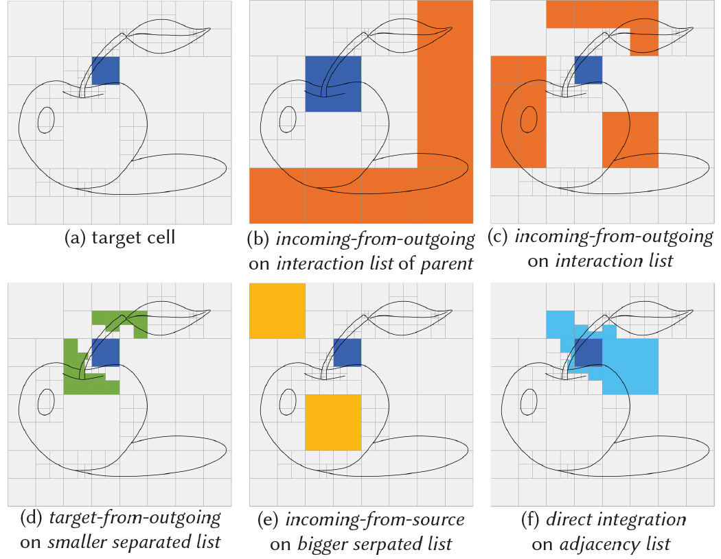
Figure 22. If a target point is contained in the blue cell (a), assuming the outgoing expansions are computed on every cell, incoming-from-outgoing expansions are computed on its interaction list from coarsest to finest (b), and transferred to its children. At its finest level, potentials are computed by summing over incoming-from-outgoing on its interaction list (c), incoming-from-incoming on its parent, target-from-outgoing on its smaller separated list (d), incoming-from-source on its bigger separated list (e), target-from-incoming from its own cell, and target-from-source (direct integration) on its adjacency list (f).

E.8. Integration of Outgoing Expansion of Green’s function

Here, we describe the analytic integration of Eq. 80. Suppose the we have a line element starting at point $p_{a}$ and ending at $p_{b}$. The integral can be expressed as:

(97) $$\hat{\bm{\sigma}}^{\beta}_{k}=\sigma\int_{p_{a}}^{p_{b}}I_{k}(p-c_{\beta})dS(p)=\sigma\bar{w}[I_{k+1}(p_{b}-c_{\beta})-I_{k+1}(p_{a}-c_{\beta})],$$

where $w$ is the complex tangential vector along the boundary $\overline{p_{a}p_{b}}$, and $\bar{w}$ its complex conjugate.

E.9. Integration of Outgoing Expansion of Normal Derivative of Green’s function

Similarly, we describe the analytic integration of the outgoing expansion of the normal derivative of the Green’s function:

(98) $$\hat{\bm{\mu}}^{\beta}_{k}=\mu n\int_{p_{a}}^{p_{b}}I_{k-1}(p-c_{\beta})dS(p)=\mu n\bar{w}[I_{k}(p_{b}-c_{\beta})-I_{k}(p_{a}-c_{\beta})].$$

E.10. Integration of Incoming Expansion of Green’s function

Here we describe the analytic integration of Eq. 83:

(99) $$\hat{\mathbf{u}}^{\alpha}_{k}=\sigma\int_{p_{a}}^{p_{b}}O_{k}(p-c_{\alpha})dS(p)=\sigma\bar{w}[O_{k-1}(p_{a}-c_{\alpha})-O_{k-1}(p_{b}-c_{\alpha})].$$

E.11. Integration of Incoming Expansion of Normal Derivative of Green’s function

Similarly, we describe analytic integration of the incoming expansion of the normal derivative of the Green’s function:

(100) $$\hat{\mathbf{v}}^{\alpha}_{k}=\mu n\int_{p_{a}}^{p_{b}}O_{k+1}(p-c_{\alpha})dS(p)=\mu n\bar{w}[O_{k}(p_{b}-c_{\alpha})-O_{k}(p_{a}-c_{\alpha})].$$

Appendix F Cost of the Single-Level Method

Here, we estimate the computational cost of the single-level method described in Section E.2. The total cost of computing the potentials can be estimated as follows, recalling that all incoming and outgoing expansions contain only $K$ terms:

• The cost of constructing all outgoing expansions is $\mathcal{O}(MK)$, since each degree of freedom in the discretization of the diffusion curves contributes to $K$ outgoing expansion coefficients of the box containing that degree of freedom.

• The cost of computing all incoming expansions from all outgoing expansions is $\mathcal{O}(K^{2}m^{2})$, since each incoming expansion coefficient of each box receives a contribution from each of the outgoing expansion coefficients of each well-separated box.

• The cost of evaluating the potential at all $N$ points using the incoming expansions is $\mathcal{O}(KN+NM/m)$, since every point receives a contribution from $K$ incoming expansion coefficients of the box containing that point, and also receives a contribution from every degree of freedom in the $\mathcal{O}(1)$ boxes in the neighbor list, each of which contains $\mathcal{O}(M/m)$ degrees of freedom.

The total cost is thus $\mathcal{O}(MK+K^{2}m^{2}+KN+NM/m)$. It is not too hard to see that this cost is minimized when the number of boxes $m$ is set to $m=(NM)^{1/3}$, which gives an overall cost of $\mathcal{O}((NM)^{2/3})$. This can be substantially better than the $\mathcal{O}(NM)$ cost of computing the potential at all $N$ points naively.

Appendix G Cost of the FMM on a Uniform Quadtree

Here, we estimate the computational cost of the FMM on a uniform quadtree described in Section E.4. The cost can be estimated as follows, once again recalling that all incoming and outgoing expansions contain only $K$ terms.

• The cost of constructing all outgoing expansion from the sources in the leaf boxes is $\mathcal{O}(KM)$, since each source point contributes to $K$ outgoing expansion coefficents in the containing cell.

• The cost of transferring outgoing expansion from the child boxes to their parents is $\mathcal{O}(K^{2}M/b(1+1/4+1/16+\cdots))=\mathcal{O}(K^{2}M/b)$, since there are $M/b$ boxes at the lowest level, $M/b\cdot 1/4$ at the next level, and so on. The exact same reasoning shows that the cost of transferring the outgoing exapnsions to incoming expansions is also $\mathcal{O}(K^{2}M/b)$, as is the cost of transferring the incoming expansions from parent boxes to child boxes.

• The cost of evaluating the potential at all $N$ target points using the incoming expansions is $\mathcal{O}(KN+Nb)$, since every point receievs a contribution from $K$ incoming expansion coefficients of the cell containing that point, and also receives a contribution from every degree of freedom in the $\mathcal{O}(1)$ boxes in the neighbor list, each of which contains $\mathcal{O}(b)$ degrees of freedom.

The total cost is thus $\mathcal{O}(KM+K^{2}M/b+KN+Nb)$. By choosing $b=K$, we have that the total cost is $\mathcal{O}(KM+KN)$, so it is linear in both the number of degrees of freedom in the sources $M$ and the number of targets $N$.

Appendix H Precomputations for the FMM

When the Fast Multipole Method is used to evaluate the potential produced by several different density functions $\sigma$ over a single set of discretized curves $\bar{S}$ and target points $q$, a large number of quantities that are independent of the density function can be precomputed. In particular, many terms appearing in the various operators used by the FMM can be precomputed. Below, we describe the precise quantities contained in the precomputatons $\mathcal{P}_{G}$ and $\mathcal{P}_{F}$ for the single- and double-layer respectively (omitting some of the quantities associated only with the FMM for the double-layer):

(101) $$\hat{\mathbf{u}}^{\alpha}_{k}=\underbrace{\int_{S}O_{k}(p-c_{\alpha})\sigma(p)dS(p)}_{\textrm{incoming-from-source}}=\sum_{i=1}^{M_{\alpha}}\bar{\sigma}_{i}\underbrace{\int_{(\bar{S}_{\alpha})_{i}}O_{k}(p-c_{\alpha})dS(p)}_{\in\mathcal{P}_{G}},$$

(102) $$\hat{\bm{\sigma}}^{\beta}_{k}=\underbrace{\int_{S_{\beta}}I_{k}(p-c_{\beta})\sigma(p)dS(p)}_{\textrm{outgoing-from-source}}=\sum_{i=1}^{M_{\alpha}}\bar{\sigma}_{i}\underbrace{\int_{(\bar{S}_{\beta})_{i}}I_{k}(p-c_{\beta})dS(p)}_{\in\mathcal{P}_{G}},$$

(103) $$\hat{\bm{\sigma}}^{\beta^{\prime}}_{k}=\underbrace{\sum_{l=0}^{k}I_{k-l}(c_{\beta}-c_{\beta^{{}^{\prime}}})\hat{\bm{\sigma}}^{\beta}_{l}}_{\textrm{outgoing-from-outgoing}}=\sum_{l=0}^{k}\underbrace{I_{k-l}(c_{\beta}-c_{\beta^{{}^{\prime}}})}_{\in\mathcal{P}_{G},\mathcal{P}_{F}}\hat{\bm{\sigma}}^{\beta}_{l},$$

(104) $$\hat{\mathbf{u}}^{\alpha}_{l}=\underbrace{(-1)^{l}\sum_{k=0}^{K}O_{l+k}(c_{\alpha}-c_{\beta})\hat{\bm{\sigma}}^{\beta}_{k}}_{\textrm{incoming-from-outgoing}}=(-1)^{l}\sum_{k=0}^{K}\underbrace{O_{l+k}(c_{\alpha}-c_{\beta})}_{\in\mathcal{P}_{G},\mathcal{P}_{F}}\hat{\bm{\sigma}}^{\beta}_{k},$$

(105) $$\hat{\bm{u}}^{\alpha}_{l}=\underbrace{\sum_{k=l}^{K}I_{k-l}(c_{\alpha}-c_{\alpha^{{}^{\prime}}})\hat{\bm{u}}_{k}^{\alpha^{\prime}}}_{\textrm{incoming-from-incoming}}=\sum_{k=l}^{K}\underbrace{I_{k-l}(c_{\alpha}-c_{\alpha^{{}^{\prime}}})}_{\in\mathcal{P}_{G},\mathcal{P}_{F}}\hat{\bm{u}}_{k}^{\alpha^{\prime}},$$

(106) $$u^{q}=\underbrace{\sum_{k=0}^{K}I_{k}(q-c_{\alpha})\hat{\mathbf{u}}^{\alpha}_{k}}_{\textrm{target-from-incoming}}=\sum_{k=0}^{K}\underbrace{I_{k}(q-c_{\alpha})}_{\in\mathcal{P}_{G},\mathcal{P}_{F}}\hat{\mathbf{u}}^{\alpha}_{k}.$$

(107) $$u^{q}=\underbrace{\frac{1}{2\pi}\sum_{k=0}^{K}O_{k}(q-c_{\beta})\hat{\bm{\sigma}}^{\beta}_{k}}_{\textrm{target-from-outgoing}}=\frac{1}{2\pi}\sum_{k=0}^{K}\underbrace{O_{k}(q-c_{\beta})}_{\in\mathcal{P}_{G},\mathcal{P}_{F}}\hat{\bm{\sigma}}^{\beta}_{k}.$$

Appendix I Pre-processing of Diffusion Curves

We pre-process input curves to lessen the burden on our adaptive subdivision algorithm. We split the curves that have intersections, and also remove (redundant) overlapping curves.