RelJoin: Relative-cost-based Selection of
Distributed Join Methods for Query Plan Optimization

Abstract

Selecting appropriate distributed join methods for logical join operations in a query plan is crucial for the performance of data-intensive scalable computing (DISC). Different network communication patterns in the data exchange phase generate varying network communication workloads and significantly affect the distributed join performance. However, most cost-based query optimizers focus on the local computing cost and do not precisely model the network communication cost. We propose a cost model for various distributed join methods to optimize join queries in DISC platforms. Our method precisely measures the network and local computing workloads in different execution phases, using information on the size and cardinality statistics of datasets and cluster join parallelism. Our cost model reveals the importance of the relative size of the joining datasets. We implement an efficient distributed join selection strategy, known as RelJoin in SparkSQL, which is an industry-prevalent distributed data processing framework. RelJoin uses runtime adaptive statistics for accurate cost estimation and selects optimal distributed join methods for logical joins to optimize the physical query plan. The evaluation results on the TPC-DS benchmark show that RelJoin performs best in 62 of the 97 queries and can reduce the average query time by 21% compared with other strategies.

[smbu]organization=Artificial Intelligence Research Institute, Shenzhen MSU-BIT University, city=Shenzhen, country=China [eipc]organization=Guangdong-Hong Kong-Macao Joint Laboratory for Emotional Intelligence and Pervasive Computing, Shenzhen MSU-BIT University, city=Shenzhen, country=China [bit]organization=School of Medical Technology, Beijing Institute of Technology, city=Beijing, country=China

[hku]organization=Department of Computer Science, The University of Hong Kong, city=Hong Kong, country=China

[hkbu]organization=Department of Interactive Media, Hong Kong Baptist University, city=Hong Kong, country=China

[fnu]organization=College of Physics and Energy, Fujian Normal University, city=Fuzhou, country=China [klqm]organization=Key Laboratory of Quantum Manipulation and New Energy Materials, city=Fuzhou, country=China [pku]organization=School of Computer Science, Peking University, city=Bejing, country=China

1 Introduction

Join query optimization is crucial for improving database query performance. Cost-based query plan optimization is an intensively studied direction in join query optimization [2, 5, 16, 20, 22, 25, 28, 32, 38] and is adopted by almost all mainstream database systems such as PostgreSQL [38] and SparkSQL [4]. Cost-based optimization usually estimates the disk I/O, CPU, and memory costs of several query plan candidates based on the statistics of the datasets and selects the one with the lowest cost estimate.

Although distributed join queries can use many traditional cost-based query plan optimization strategies that are designed for a single computer node, they face unique challenges owing to their distributed nature. First, physical methods for distributed joins are more complicated than those of local joins. A distributed join involves a data exchange phase [4, 5] in which data are transferred to different partitions via the communication network before the local join operation is executed in each node. Instead of planning a sort join or hash join for local joins, the query planner for distributed joins has other options, including the broadcast hash join, shuffle hash join and shuffle sort join. Different physical join methods may perform completely differently. Second, the network communication cost, or network cost, is a non-negligible part of the total cost, which complicates the cost model. Broadcasting a complete replicate of a table for all nodes in a large cluster or shuffling the data of a large table inevitably incurs considerable network traffic. This network cost may be substantial for large datasets or clusters, which can result in a performance bottleneck for distributed operations that require data repartitioning [23, 31]. The cost model must also properly assign weights to the network and other resource costs. Third, the consequences of using biased dataset statistics for cost estimation can be amplified in distributed joins. For example, if the size-related statistics of a large table are mistakenly estimated as small, the query optimizer may select the incorrect join order or method. An inferior choice between the sort and hash methods may result in little performance difference in local joins [6], whereas broadcasting a large table instead of shuffling it can be disastrous for distributed joins [11].

Therefore, a precise cost model is imperative to select the best physical join method for distributed joins. Several studies on cost-based optimization (CBO) have focused on logical join order optimization [14, 20, 28, 34, 39] because local joins can benefit immensely from the optimal join order. For distributed joins, the network cost accounts for the majority of the total cost, and selecting the proper distributed join method is critical for query performance. An increasing number of studies [33, 41] have focused on comprehensive costs in distributed environments. Many cost models [5, 17, 18, 22, 29, 30] also highlight the network cost; however, they are not primarily designed for a scalable environment and rely on some inputs that can be easily derived in data-intensive scalable computing (DISC) platforms, or they involve abundant hyperparameters that are specific to the complex scalable environment and face potential practical problems.

We aim to design and implement a precise and practical cost model for distributed joins that appropriately addresses the network and computing costs of DISC platforms. We propose RelJoin, which is an adaptive cost-based query optimization strategy for selecting distributed join methods when deciding on a physical query plan, and seamlessly integrate it as a physical plan optimization rule in SparkSQL, which is an industry-prevalent big data processing platform. The RelJoin source code is open for access. It has the following features that are specifically designed to tackle problems with cost-based distributed join method selection. First, the cost model incorporates the network and computing workloads of different joining phases of different physical distributed join methods in the cluster. The cost model is precise and simple with only one hyperparameter to weight the network workload against the computing workload, where the network workload depends on the data sizes, communication pattern, and cluster configuration. Second, the statistics of the datasets that are used for the join method cost model are adapted from actual runtime statistics of every data exchange phase, which enables close-to-fact cost estimation. During the data exchange phase of every join or group-by-like operation, the query optimizer collects the runtime statistics of the output dataset including the cardinality and size. The optimizer adapts the output statistics of the successor operations based on the phase-updated runtime statistics and uses the adapted runtime statistics for the cost calculation in the subsequent join operation. Third, the physical query plan can be efficiently re-optimized during its execution based on the adaptive runtime statistics. With such statistics adaptively updated based on the runtime results, the physical query plan is re-optimized by re-selecting better physical methods for the remaining joins.

The evaluation results show that RelJoin accurately selects the distributed join methods and thus significantly improves the performance of join queries in TPC-DS [1], which is an industry-standard database test suite for big data processing platforms. Furthermore, the relative size of the joining datasets is a better criterion than the absolute size for judging whether a broadcast or shuffle join method costs less and is hence a preferable option for a logical join. We further propose the Performance Sensitivity To Selection (PSTS) as a general metric to measure the optimization effectiveness of join method selection strategies in different benchmarks, and show that RelJoin effectively optimizes the query plan by selecting the best join methods. The major contributions of this study are summarized as follows:

• We build a cost model of various distributed join methods with different communication patterns and in-memory operations and highlight the importance of the relative size of joining datasets when comparing different distributed join methods. Our cost model is robust in data skew scenarios and particularly practical for the complex distributed environment as it has only one hyperparameter which is the relative weight of the network cost of the distributed join method.

• We propose RelJoin query optimization strategy and seamlessly implement it in SparkSQL. This strategy selects the best distributed join methods based on adaptive runtime statistics and efficiently re-optimizes the physical query plan.

• Our evaluation results show that RelJoin can reduce the TPC-DS query completion time by 21% and achieve the best performance in 62 of the 97 queries compared with other available join method optimization strategies. We also propose the novel PSTS as a general metric for measuring the optimization effectiveness of various join method selection strategies.

The remainder of this paper is organized as follows. Section 2 presents the background on distributed join methods and distributed query optimization. In Section 3, we model, analyze, and compare the costs of various distributed join methods in different joining phases. We describe the optimization framework of RelJoin and the implementation details in Section 4 and present the evaluation results for the TPC-DS benchmark in Section 5. Section 6 outlines the related work, and Section 7 concludes the paper and notes the plans for future work.

2 Background

2.1 Distributed join methods

Various physical implementation methods are available for a logical join operation depending on the computing paradigm. In contrast to local join operations that join data within a computing node, the implementation of distributed operations involves an additional data exchange phase that rearranges data locations across nodes via the network prior to the join. Distributed join methods vary according to their implementation methods in the data exchange and local join phases. For simplicity, we use the word “join” to refer to a logical join operation or physical join method, depending on the context.

2.1.1 Broadcast and shuffle

Two main methods are used in the data exchange phase. The broadcast method sends an entire replicate of the smaller table on one side of the join operation to all nodes in the cluster, whereas the data of the other table remain unmoved. This can be viewed as the cross-node version of replicating small tables in multiple cores [11]. The shuffle method partitions both tables based on the hash values of the join keys and relocates their data partitions to the corresponding nodes. The network costs are a major concern when comparing these two methods. In general, the broadcast method may perform better when the table to be broadcast is sufficiently small, whereas the shuffle method is preferred when both tables are large. The data rows that are required for a local join at each node should be ready following the data exchange phase.

2.1.2 Hash, sort, and nested loop

The hash, sort, and nested loop are typical methods for the local join phase that handle the partitioned table data at each node. The hash join [12] first builds a hash map for the smaller table and then probes the hash map to identify the matching rows for each row in the larger table. This requires additional memory space to store the hash map. The sort join [3], which also known as the sort-merge join, first sorts both tables using the join key and then merges the two sorted tables. Both the hash and sort methods are only used in equi-joins, and the sort method requires the join key to be sortable. The nested loop join simply uses two loops over all rows in both tables to identify the matching rows. This method is inefficient and should not be selected unless the hash and sort joins are infeasible.

There is a debate over which of the hash and sort methods is more efficient. The answer depends on various factors including the CPU and memory architecture and the in-memory implementation. In generally, a hash join is considered as the default join method [7, 19]. The sort join performs better when wide SIMD instructions and NUMA access are available [6]. Our cost model ranks the hash method higher than the sort method (Section 3.6); however, our results (Section 5.3) show that the performance difference between them is so small that the choice can be flexible.

In this study, we focus on discussing only certain often-used distributed join methods, such as the broadcast hash join, shuffle hash join and shuffle sort join. We find that the choice between broadcast and shuffle has a much greater impact on the performance than the choice between hash and sort.

2.2 Distributed query optimization

A query is parsed into a tree structure to direct the execution of a series of data transformation operations for logical and physical query plans in many distributed database systems [4, 36]. To achieve better performance, the query optimizer analyzes, rewrites, and optimizes both the logical and physical plans by applying some well-studied optimization rules and cost models [10, 16]. In this study, we use the terms query plan and plan interchangeably.

A logical plan is an abstract picture of the structure and sequence of a series of logical operations, such as join, filter and groupBy. It determines the output result of a query but does not specify the implementation method for each operation. Various intermediate logical plans that can output the same query results are generated; however, only the optimal plan is eventually selected to generate the physical plans.

Once the optimized logical plan is ready, the system translates it into a physical plan that defines the detailed physical methods used for each logical operation. The plan optimizer can directly determine the best physical method for a logical operation by following pre-defined rules. The optimizer may also generate a set of physical plans each of which represents a possible combination of physical methods from the logical plan, and select the optimal physical plan based on a cost model. Finally, the optimized physical plan is used to generate code that can be executed in the distributed database system. However, it may also be re-optimized at runtime using updated statistics or configurations.

In this study, we use a precise cost model to select the best distributed join methods for logical join operations and to optimize the physical plan. Using the cost model to optimize join orders is a traditional topic under local joins, which has been studied extensively in the context of traditional database systems, and thus, is not the focus of this study.

2.3 Adaptive statistics and the cost model

The cost model for the query optimizer requires the statistics of the input datasets to estimate the operational costs. Using the statistics of the input datasets, the optimizer can statically analyze the statistics of the output dataset for every operation along the logical plan [2]. These statistics usually include the cardinality, size, and some column-specific statistics, such as the distributions of column values. The analyzed statistics are approximate estimates and may deviate significantly from the actual dataset following a sequence of operations along the query plan. Biased statistics may result in incorrect optimization decisions.

Adaptive runtime statistics [13] provide more close-to-fact estimates of the cost model than statically analyzed ones. Distributed computing paradigms [4, 36] typically separate the query plan into several query stages, where the data exchange phase of a shuffle-like operation is the synchronization barrier between the query stages of parallel tasks in all nodes. The query plan optimizer can update the statistics of the datasets to actual runtime statistics during the execution of every data exchange phase so that the dataset statistics are expected to be runtime-accurate at the beginning of every query stage. The optimizer uses the updated runtime statistics as a starting point to estimate the statistics of the output datasets for successor operations in the new query stage, which we refer to as adaptive runtime statistics in this study. Our proposed cost model uses adaptive runtime statistics as the inputs, leading to precise cost estimates for distributed join methods and optimal method selection decisions. The physical plan is re-optimized based on the phase-updated adaptive runtime statistics.

Join cost models [9, 25] usually formulate the costs of different types of resources (e.g., disk, memory, and CPU) or access patterns (e.g., sequential and random access) in different execution phases. The cost of the distributed join methods should consider the network cost in the data exchange phase and other computing costs in the local join phase.

In this study, we use adaptive runtime statistics to formulate the costs of the different phases of various distributed join methods, with special consideration of the network cost.

3 Cost models

In this section, we discuss the modeling assumptions and model the costs of various distributed join methods. We provide insights into the cost comparisons of these distributed join methods and the data skew problem.

3.1 Modeling assumptions

3.1.1 Metrics

Certain studies have modeled the query completion time [5, 9] or workload of a node with multiple cores [25] as a metric to estimate the cost of a join method. In this study, we use the cluster workload of different phases, which measures the volumes of the input datasets and related computational and communication complexities in the cluster, as the cost metric with the following considerations: First, the workload estimation is simple but more accurate. It does not require detailed information such as the processing speed of all related computing, I/O resources, and access patterns, which vary in different environments and are usually difficult to represent precisely. Second, data skew is not a severe problem in cluster workload estimation. By summing up the workload of each node with skewed data, the skewed cluster workload would be close to the cluster workload as if the data were evenly distributed in the cluster, especially when the cluster has many parallel tasks. As a comparison, the completion time estimation is determined by the last finished task, which is known as the straggler, and requires the global data distribution statistics. Third, as the paradigms of various distributed join methods can be uniformly abstracted to the combination of data exchange and local join phases, where the performance of each phase is dominated by the same resource type (i.e., computational and communicational), the cluster workloads of each phase of the different distributed join methods are easily comparable.

3.1.2 Workload

The workload in the data exchange phase is the network communication workload, or network workload. The workload in the local join phase involves the use of computing resources in the local node, including the CPU, memory, and disk if data are spilled or virtual pages are swapped. We summarize this workload as the computing workload.

3.1.3 Data distribution

Collecting the global distribution histogram statistics is expensive. Fortunately, with the cluster workload as the metric, assuming that the data are uniformly distributed would generate an approximate result that is sufficient for cost comparison [8, 9], while simplifying the cost model and reducing the optimization overhead. We first assume a uniform data distribution across nodes in the cluster in each phase and use the cluster workload to measure the cost of the distributed join methods. In Section 3.7, we later analyze the influence of skewed data on the cost model to show that our model is invariant when data skew exists.

Table 1: Model notations

Notation	Description	Notation	Description
$|A|$	the size of $A$	$|B|$	the size of $B$
$a$	the cardinality of $A$	$b$	the cardinality of $B$
$|A|/a$	the row size of $A$	$|B|/b$	the row size of $B$
$|A|/p$	the partition size of $A$	$|B|/p$	the partition size of $B$
$a/p$	the cardinality of a partition of $A$
$b/p$	the cardinality of a partition of $B$
$l_{fan}$	the average # of matching rows in $B$ for each row in $A$
$w$	the relative weight of the network cost against the
	computing cost
$k$	the relative size coefficient of $A$ and $B$, where $|A|=k|B|$
$n$	the number of cluster nodes
$p$	distributed join parallelism
Notation	The cluster (network/computing) workload of …
$C_{broadcast}$	(network) broadcasting a dataset in broadcast hash join
$C_{build}$	(computing) building the hash map in broadcast hash join
$C_{probe}$	(computing) probing the hash map in hash joins
$C_{shuffle}$	(network) shuffling partitions in shuffle joins
$C_{sort}$	(computing) sorting partitioned data in shuffle sort join
$C_{merge}$	(computing) merging sorted partitions in shuffle sort join
$C^{\prime}_{build}$	(computing) building the hash map in shuffle hash join
$C_{NL}$	(computing) nested loop in broadcast nested loop join

3.1.4 Problem setting

We model the cost of a distributed equi-join of datasets $A$ and $B$, which runs in a cluster of $n$ nodes, where each node runs several executors to perform the data exchange and local join tasks in parallel. Each task handles a partition of the dataset. Suppose that the number of shuffle partitions for the join is $p$, which is known as the distributed join parallelism. The notations are listed in Table 1 for ease of reference. Assume that $|A|\geq|B|$. We use the larger dataset to join the smaller dataset. Thus, datasets $A$ and $B$ are located on the left and right sides of the join, respectively. The cardinalities of $A$ and $B$ are substantially higher than the distributed join parallelism; that is, $a\gg p$ and $b\gg p$. Both datasets are uniformly distributed to the partitions. The average number of matching rows in dataset $B$ for each row in dataset $A$, which is known as the fanout level of $A$, is denoted as $l_{fan}$. We assume that the join keys are sortable so that the sort join is feasible.

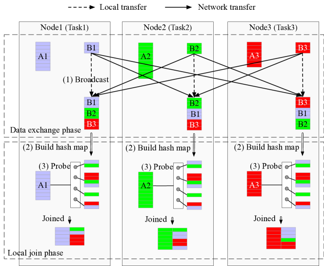
Figure 1: The broadcast hash join

3.2 Broadcast hash join

Fig. 1 depicts the broadcast hash join procedure for datasets $A$ and $B$, with three nodes in the cluster and one task in each node. It comprises three steps: broadcast, build, and probe.

3.2.1 Broadcast

In the data exchange phase, all $p$ tasks collect the entire replicate of the smaller dataset $B$. In each task, $1/p$ of the dataset already resides in that task process and can be used directly (the dashed arrows of Step 1 in Fig. 1), and $(p-1)/p$ of the dataset is retrieved from other tasks either in the same node or nodes across the network (the solid arrows of Step 1 in Fig. 1). Although fetching a partial dataset from other tasks in the same node via the network interface can be optimized via the local disk or shared memory access, this is usually considered network I/O in practice. Therefore, the workload of each task in the broadcast step is $|B|(p-1)/p$, and the cluster network workload of $p$ tasks is

$$C_{broadcast}=(p-1)|B|.$$ (1)

3.2.2 Build

In the local join phase, each task first builds a hash map for the entire dataset $B$ (Step 2 in Fig. 1) to accelerate the later probe step. The workload for building the hash map for each task is $|B|$, and the cluster computing workload is

$$C_{build}=p|B|.$$ (2)

3.2.3 Probe

In the probe step, the task traverses each row in a partition of dataset $A$, where the partition cardinality is $a/p$, and probes the hash map to identify matching rows with the same key value in the entire dataset $B$ (Step 3 in Fig. 1). The workload of each task depends on the fanout level of $A$, $l_{fan}$. It visits rows of size $|A|/a$ $a/p$ times and those of size $|B|/b$ $al_{fan}/p$ times. The cluster workload of the probe is

$$C_{probe}=p(\frac{a}{p}\frac{|A|}{a}+\frac{al_{fan}}{p}\frac{|B|}{b})=|A|+\frac{al_{fan}}{b}|B|.$$

In the best case, when no rows in dataset $A$ can find a matching row and $l_{fan}=0$, the cluster workload is simply traversal of all rows in dataset $A$ and is $|A|$. In the worst case, when the key values of all rows in datasets $A$ and $B$ are the same and each row on the left of the join matches all rows on the right, $l_{fan}=b$. The cluster workload is $|A|+a|B|$. On average, we can assume that the matching rows of all $a$ rows in $A$ are evenly distributed across all $b$ rows in $B$, and we obtain $l_{fan}=b/a$. Therefore,

$$C_{probe}=|A|+|B|$$ (3)

3.2.4 Overall

Recall that the broadcast workload is the network cost, and the build and probe workloads are the computing costs. We assign different weights to these costs of different resource types when combining them to obtain the overall cost. As only two resource types are considered, instead of assigning each cost with a weight coefficient, that is, $w_{1}$ and $w_{2}$, we use a single variable $w$ to denote the relative weight of the network cost against the computing cost for simplicity. Using Equations 1, 2, and 3, the overall cost of the broadcast hash join is

$$C_{broadcastHash} =wC_{broadcast}+C_{build}+C_{probe}$$ (4)

$$=|A|+(wp-w+p+1)|B|.$$

This is a linear function of the sizes of datasets $A$ and $B$.

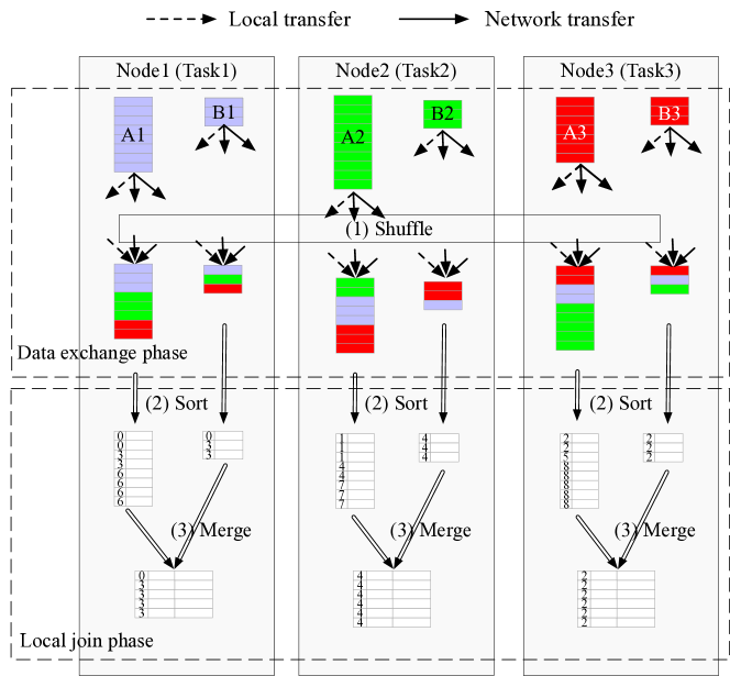
Figure 2: The shuffle sort join

3.3 Shuffle sort join

Fig. 2 depicts the procedure of the shuffle sort join of datasets A and B with three nodes in the cluster and one task in each node. This process comprises three steps: shuffle, sort, and merge.

3.3.1 Shuffle

In the shuffle step, both datasets are repartitioned across tasks via the network (Step 1 in Fig. 2). As in the broadcasting, $1/p$ of the partition data are process-native and $(p-1)/p$ are retrieved via the network in each task. The difference is that in the broadcast step, each task needs to collect the entire dataset $B$, whereas in the shuffle step, each task only collects a partition of datasets $A$ and $B$. Therefore, the workload of each task in the shuffle step is $((p-1)/p)(|A|/p+|B|/p)$. The cluster network workload of $p$ tasks is

$$C_{shuffle}=\frac{p-1}{p}(|A|+|B|).$$ (5)

3.3.2 Sort

In the sort step, each task sorts a partition of datasets $A$ and $B$ (Step 2 in Fig. 2), respectively. To sort a partition of $A$ with $a/p$ rows where the size of each row is $|A|/a$, the workload is $\frac{|A|}{a}\frac{a}{p}\log_{2}\frac{a}{p}$, or $\frac{|A|}{p}\log_{2}\frac{a}{p}$. The workload for sorting a partition of $B$ can be derived in a similar manner, and the workload of each task in the sort step is $\frac{|A|}{p}\log_{2}\frac{a}{p}+\frac{|B|}{p}\log_{2}\frac{b}{p}$. The cluster computing workload is

$$C_{sort}=|A|\log_{2}\frac{a}{p}+|B|\log_{2}\frac{b}{p}.$$ (6)

3.3.3 Merge

To merge two sorted partitions of datasets $A$ and $B$, the workload is simply the sum of the sizes of these two partitions; that is, $|A|/p+|B|/p$ for each task. The cluster computing workload in the merge step is

$$C_{merge}=|A|+|B|.$$ (7)

3.3.4 Overall

Similar to the overall cost of the broadcast hash join, we assign a weight $w$ to the network cost in the shuffle phase. Using Equations 5, 6, and 7, the overall cost of the shuffle sort join is

$$C_{shuffleSort}=wC_{shuffle}+C_{sort}+C_{merge}$$ (8)

$$=(\frac{wp-w+p}{p}+\log_{2}\frac{a}{p})|A|+(\frac{wp-w+p}{p}+\log_{2}\frac{b}{p})|B|.$$

The result depends not only on the sizes of both datasets, but also on the cardinalities owing to sorting.

3.4 Shuffle hash join

For the shuffle hash join, the shuffle step is identical to that of the shuffle sort join, as is the corresponding cluster workload, which is $C_{shuffle}$ in Equation 5. The local join phase follows the same pattern as the broadcast hash join; however, the input sizes of the datasets for the build and probe steps differ.

In the build step for each task, instead of building the hash map for the entire dataset $B$ of size $|B|$ as in the broadcast hash join, the task only needs to build the hash map for a partition of dataset $B$ which is of size $|B|/p$. Therefore, the cluster computing workload of this build step is

$$C^{\prime}_{build}=|B|.$$ (9)

In the probe step, although the size of the hash map in a task is only $1/p$ of that in the broadcast hash join, the workload depends only on the cardinality of the partition of $A$, row sizes of $A$ and $B$, and fanout level of $A$. Therefore, the cluster probe workload of the shuffle hash join is the same as that of the broadcast hash join, which is $C_{probe}$ in Equation 3.

Using Equations 3,  5, and 9, with weight $w$ assigned to the shuffle workload, the overall cost of the shuffle hash join is

$$C_{shuffleHash} =wC_{shuffle}+C^{\prime}_{build}+C_{probe}$$ (10)

$$=\frac{wp-w+p}{p}|A|+\frac{wp-w+2p}{p}|B|.$$

It is also a linear function of the sizes of datasets $A$ and $B$.

3.5 Broadcast nested loop and Cartesian product joins

We introduce two variants of distributed join methods that are used only when the above methods are infeasible, and discuss the reason for their poor performance based on the cost model. These are the broadcast nested loop join (broadcast NL join) and Cartesian product join. They should not be selected except when the join is not an equi-join, the join key is not sortable, or there is insufficient space to build the hash map.

For the broadcast NL join, the data exchange phase is the same as that of the broadcast hash join, which is the broadcast step. In the local join step, each task loops over all rows of a partition of dataset $A$, and for this every row, loops over all rows in the entire replicate of dataset $B$. The outer loop runs $a/p$ times and visits rows of size $|A|/a$. The inner loop runs $ab/p$ times and visits rows of size $|B|/b$. The cluster NL workload is

$$C_{NL}=p(\frac{a}{p}\frac{|A|}{a}+\frac{ab}{p}\frac{|B|}{b})=|A|+a|B|.$$ (11)

We can easily determine why the broadcast NL join method is inferior to other distributed join methods by comparing their local join workloads. For example, according to Equations 2 and 3, the cluster workload of the local join phase of the broadcast hash join is $C_{build}+C_{probe}$; that is, $|A|+(p+1)|B|$. As the dataset cardinality $a$ is assumed to be significantly larger than $p$, $C_{NL}\gg C_{build}+C_{probe}$.

Using Equations 1 and 11, the overall cost of the broadcast NL join is

$$C_{broadcastNL} =wC_{broadcast}+C_{NL}=|A|+(wp-w+a)|B|.$$

Logically, the Cartesian product join is a shuffle NL join. The data exchange phase is a shuffle step and its cluster workload is $C_{shuffle}$. The NL step is similar to that of the broadcast NL join; however, the inner loop only visits a partition of dataset $B$, which has $b/p$ rows instead of ${b}$ rows. Therefore, the inner loop runs $a/p\times b/p$ times instead of $ab/p$ times. Everything else remains the same as in the broadcast join in the NL step, and the cluster NL workload of the Cartesian product join is

$$C^{\prime}_{NL}=p(\frac{a}{p}\frac{|A|}{a}+\frac{ab}{p^{2}}\frac{|B|}{b})=|A|+\frac{a}{p}|B|.$$ (12)

We can also find that the Cartesian product join is inferior to the shuffle hash join by comparing their local join workloads. According to Equations 3 and 9, the local join workload of the shuffle hash join is $C^{\prime}_{build}+C_{probe}$, which is $|A|+2|B|$. When $a/p\gg 2$, $C^{\prime}_{NL}\gg C^{\prime}_{build}+C_{probe}$.

According to Equations 5 and 12, the overall cost of the Cartesian product join is

$$C_{cartesian} =wC_{shuffle}+C^{\prime}_{NL}$$

$$=\frac{wp-w+p}{p}|A|+\frac{wp-w+a}{p}|B|.$$

3.6 Comparison

We discuss and provide insights into the cost models of the broadcast hash join, shuffle hash join, and shuffle sort join.

3.6.1 Shuffle hash vs. shuffle sort

Although the hash and sort method are considered as comparable join methods, in our cost model, the hash method always has a lower workload than the sort method. It can be inferred from Equations 3, 6, 7, and 9 that $C^{\prime}_{build}+C_{probe}<C_{sort}+C_{merge}$. Therefore, provided that there is sufficient memory to create a hash map for a partition of $B$, our cost model always prefers the shuffle hash join. However, note that the additional memory space that is occupied by the shuffle hash join is not considered in the cost model.

3.6.2 Broadcast hash vs. shuffle hash

The workloads of these two methods differ not only in the data exchange phase but also in the local join phase. These can be compared by simply calculating their overall costs. As both costs are linear functions of $|A|$ and $|B|$, we can reformulate the costs by exploring the relative sizes of datasets $A$ and $B$.

Let $|A|=k|B|$, where $k$ represents the relative size coefficient of datasets $A$ and $B$. If $k=k_{0}$ and $C_{broadcastHash}=C_{shuffleHash}$, solving this equation using Equations 4 and 10, we have

$$k_{0}=\frac{pw+p-w}{w}.$$ (13)

When $k\leq k_{0}$, $C_{broadcastHash}\geq C_{shuffleHash}$. When $k>k_{0}$, $C_{broadcastHash}<C_{shuffleHash}$. The value of $k_{0}$ is proportional to the value of $p$. The relative costs of these two join methods are directly determined by the relative size coefficient $k$, distributed join parallelism $p$, and network cost relative weight $w$.

This result is consistent with our intuition regarding the costs of the two distributed join methods. When $A$ is not sufficiently large relative to $B$, the workload of shuffling both datasets is not heavy compared with that of broadcasting $B$. Furthermore, the shuffle method builds a smaller hash map than the broadcast method does. In this case, the shuffle hash join may is preferred. However, when $A$ is sufficiently larger than $B$, with a relative size coefficient that is larger than a particular threshold, shuffling the large dataset $A$ can become a heavier workload than broadcasting the entire replicate of $B$ and building the hash map for it. In this case, the broadcast hash join is preferred. $k_{0}$ is the threshold at which $A$ is considered sufficiently bigger than $B$. When the number of parallel join tasks is larger, the cost of broadcast $B$ is greater, and the threshold should be higher for $A$ to be considered large. As mentioned in Section 2.2, SparkSQL uses a manually set absolute size to determine whether a dataset is sufficiently small for broadcasting. Our cost model indicates that the relative size is the criterion for selecting the broadcast or shuffle method.

3.7 Analysis of data skew

The cost model assumes a uniform data distribution across the nodes. Although considering data skew complicates the cost model, but we can briefly discuss its influence on the current cost model if data skew is considered. Inferior nested-loop-like joins are not discussed here.

The overall cluster workload of the broadcast hash join ($C_{broadcastHash}$ (4)) remains unchanged. When the cluster workload of a step of a distributed join explains the expected sum of the partition data sizes, with every partition weighted by the same constant value, the cluster workload remains the same even if the dataset is skewed across the nodes. This is the case with $C_{broadcast}$ (1), $C_{build}$ (2), $C_{probe}$ (3), $C_{merge}$ (7), and $C^{\prime}_{build}$ (9).

The overall cluster workload of the shuffle hash join ($C_{shuffleHash}$ (10)) also remains unchanged. The shuffle workload is not affected by the data distribution but by the data key dependency between the join input and output [23]. In Section 3.3.1, our cost model implicitly implies the data key dependency by assuming that $(p-1)/p$ of each partition data will be transferred via the network. In extreme cases, when all data rows are already in the nodes where they will be processed later, no data must be shuffled, and $C_{shuffle}=0$. In contrast, if all data in both datasets are not in the nodes where they will be processed and the entire dataset needs to be transferred via the network, $C_{shuffle}=|A|+|B|$. In the data skew case, if the same data key dependency assumption is held, the cluster workload of the shuffle step $C_{shuffle}$ (5) is the same as that of the uniformly distributed case.

The sort-step workload and thus the overall cluster workload of the shuffle sort join will be higher. The cluster workload of the sort step contains the expected sum of the products of the partition cardinality and the logarithm of the partition cardinality, which has the minimum value when the cardinalities of all partitions are the same in the uniform distribution case. When the data are skewed, it is higher than $C_{sort}$ (6). The higher cost of the shuffle sort join in the data skew case does not change its rank compared to the shuffle hash join, which is preferred by our model.

That is, considering data skew does not affect the comparable costs of the distributed join methods in our cost model.

Table 2: A summary of the costs of different distributed join methods with the suffixes of $C$ indicating the method types and their ranks (higher-rank methods are preferred when they are feasible)

Join method	Cost	Rank
$C_{broadcastHash}$	$|A|+(wp-w+p+1)|B|$	3
$C_{shuffleSort}$	$(\frac{wp-w+p}{p}+\log_{2}\frac{a}{p})|A|+(\frac{wp-w+p}{p}+\log_{2}\frac{b}{p})|B|$	2
$C_{shuffleHash}$	$\frac{wp-w+p}{p}|A|+\frac{wp-w+2p}{p}|B|$	3
$C_{broadcastNL}$	$|A|+(wp-w+a)|B|$	1
$C_{cartesian}$	$\frac{wp-w+p}{p}|A|+\frac{wp-w+a}{p}|B|$	1

3.8 Cost summary

The costs and the rankings of the different distributed join methods mentioned above are summarized in Table 2. Of all feasible join methods for a specific logical join, the join methods are selected based on the rank first and cost size later. The join method with the highest rank and lowest cost is selected, as explained in the following section.

4 Cost-based optimization framework

In this section, we describe the query optimization framework of RelJoin which incorporates the cost model to select the best distributed join method based on adaptive runtime statistics. We also introduce the details of the implementation of RelJoin in SparkSQL.

4.1 Optimization procedure

Fig. 3 depicts the optimization procedure of RelJoin. The tree with dashed nodes represents an optimized logical query plan, and the tree with solid nodes represents the (re-)optimized physical query plan. As mentioned in Section 2.3, a query plan is divided into query stages. The nodes in the dark background are data exchange operations that act as the boundaries of the query stages. In Step 1, every query stage is executed according to the optimized physical plan, and the runtime statistics of the corresponding operation nodes in the logical query plan are updated. According to our cost model, the required statistics are the size and cardinality of the output dataset. In Step 2, the logical plan adapts the updated runtime statistics along the query path until it reaches the next data-exchange operation, such as a join operation. In Step 3, for this logical join operation, the cost model uses the adaptive runtime statistics to select the best distributed join method for the current stage and generates a new optimized physical plan. This step is known as the re-optimization of the physical plan, which we will discuss further. In Step 4, the execution of the distributed join collects the runtime statistics of the output for the re-optimization of the next stage starting from Step 2. This procedure is iterated until it reaches the root of the query plan and retrieves the final result.

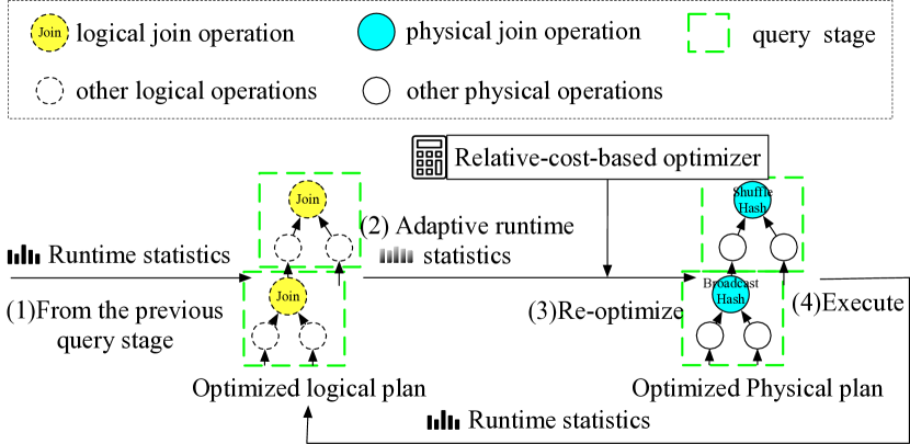
Figure 3: The adaptive cost-based join method optimization procedure

4.2 Optimization time complexity

The physical plan optimization for the distributed join method selection in RelJoin is time efficient. In certain cost-based optimization strategies [2], the optimizer generates many alternative plans, each of which is a possible combination of the choice results for a sequence of join operations. Subsequently, it uses a cost model to select the best one with the lowest cost. Determining the globally optimal plan in this manner is an NP-hard problem. For example, for a query plan with $h$ successive joins, where each join has $l$ physical methods for selection, the time complexity for determining the globally optimal plan for the above strategy is $O(l^{h})$. In our setting, where the data are uniformly distributed across the cluster, because the cost of a distributed join method for every logical join is independent of the costs of other logical joins, the optimization of a logical join is independent of the optimization of the others. In every physical plan re-optimization iteration in RelJoin, the optimizer only independently determines the optimal join method for the corresponding logical join to be executed. A globally optimal plan is generated and executed after $h$ optimizations or re-optimizations of the physical plan. The time complexity is $O(lh)$, which is a time-efficient polynomial.

4.3 Distributed join method selection

We describe the algorithm for using the cost model to select the best distributed join method for a logical join in every iteration of the physical plan optimization or re-optimization. Algorithm 1 presents the brief selection algorithm for an equi-join, in which two datasets are joined based on equality or matching column values. When no user-defined hint is provided for the selection preference, the optimizer calculates the costs of various distributed join methods. It selects the join method with the lowest cost permitted by the join type and memory requirements. The best distributed join method for this logical join is returned. In the algorithm, the shuffle hash join is ranked higher than the shuffle sort join, and the hash- and sort-based joins are ranked higher than the NL-based joins.

If a non-equi-join is inner-like, as only the Cartesian product join and broadcast NL join are feasible, the optimizer selects the join method with the lower cost.

Input: the logical equi-join

Input: the cost model that return the cost of different distributed join methods for a logical join

Output: the distributed join method

1

2if the user-defined join hint exists in the logical join then

3       return the hinted join method

4 end if

5

6$C_{broadcastHash}$ = the broadcast hash join cost

7 $C_{shuffleHash}$ = the shuffle hash join cost

8

9if $C_{broadcastHash}<C_{shuffleHash}$ and hashing is allowed then

10       return the broadcast hash join

11 else if hashing is allowed then

12       return the shuffle hash join

13 else if the join key is sortable then

14       return the shuffle sort join

15 else

16       $C_{broadcastNL}$ = the broadcast NL join cost

17       $C_{cartesian}$ = the Cartesian product join cost

18       if $C_{cartesian}\leq C_{broadcastNL}$ and the join type is inner-like then

19             return the Cartesian product join

20       else  return the broadcast NL join

21      

22

Algorithm 1 Cost-based distributed join method selection

4.4 Implementation details

We implement RelJoin in SparkSQL as a physical plan optimization rule. Consequently, RelJoin automatically applies the optimization mechanisms that are already implemented by SparkSQL, including the adaptive runtime statistics and the physical plan re-optimization. The following implementation factor are considered:

• Backward compatibility: RelJoin should be compatible with the original join method selection strategy and other query plan optimization techniques.

• Data reliability: RelJoin should measure the join operation costs and make selections based on reliable input statistics.

• User friendly: RelJoin should be seamlessly implemented on the platform and can be used by users with minimum learning effort.

The respective implementation details for dealing with these considerations are as follows.

First, RelJoin is implemented in the same physical plan optimization rule where the original distributed join method selection strategy is implemented such that either RelJoin or the original strategy can run alongside other query optimization techniques. The original join selection strategy follows an absolute-size approach, which prefers the broadcast method over the shuffle method when the size of the smaller dataset is within a user-defined absolute value, such as 10 MB. When RelJoin is configured to be enabled, the original strategy is switched to RelJoin unless the statistics are invalid, as described below.

Second, the statistics are not always ready or meaningful for an operation, particularly in the first query stage. For example, because of the lazy execution mechanism, when loading a dataset from a data source that does not have statistics in the header, the optimizer cannot provide a proper estimate of the statistics and initializes the dataset size statistics to a very large number. Using the adaptive statistics from this initialized value for the cost model will lead to incorrect join method selection decisions, such as broadcasting and building a hash map for a very large dataset. To address this problem, RelJoin treats only size statistics below a watermark number as valid statistics. This watermark is the largest dataset size that is supported the RelJoin strategy, and we set it to 100 GB by default. In the case of invalid statistics for a logical join, RelJoin switches to the original join selection strategy for that join. The original strategy may simply think that the datasets are too large for broadcasting and hashing, and select the sort merge join.

Third, the weight of the network cost relative to the computing cost $w$ is user configurable. This is the only variable in RelJoin that depends on the environment. In Section 5.5, we demonstrate that RelJoin performs well with different $w$ values and users do not need to spend much time tuning this parameter.

5 Evaluation

In this section, we present the performance evaluation results of RelJoin based on the TPC-DS benchmark and compare them with those of other join method selection strategies. The results show that RelJoin improves the query time significantly by selecting the best distributed join methods. We statistically analyze the query plans and discuss the insights and key factors that make RelJoin a better optimization strategy. We also explore the impact of different values of the relative weight of the network cost on the computing cost, $w$.

Table 3: (a) Evaluation benchmark specifications (the scale, the raw text size of the whole benchmark, and the raw text size of the largest dataset in the benchmark), testbed executor and node resource capacity configurations; (b) excluded queries for the benchmarks of each scale; and (c) strategies for distributed join method selection

Scale	Whole size	Largest size	Node	Executor
1	1.2 GB	386 MB	16 GB	4 GB/1 core
10	12 GB	3.7 GB	32 GB	14 GB/2 cores
100	96 GB	38 GB	32 GB	14 GB/2 cores
Scale	Excluded queries			# Queries
1	q10, q35, q69 for AQE and RelJoin			97
10	q10, q35, q69, q72 for all			93
100	q10, q14a, q14b, q35, q37, q69, q72 for all			90
Strategy	Description
ShuffleSort	Force to select the shuffle sort join if keys are sortable.
ShuffleHash	Force to select the shuffle hash join if the dataset is
	small enough for building the hash.
AQE	Select the broadcast hash join if the size of the adaptive
	runtime statistics of a dataset does not exceed 10 MB.
	Otherwise, select the shuffle hash or shuffle sort join.
RelJoin	Network workload weight $w=1$ and hence $k_{0}=39.$

5.1 Benchmark, testbed, and metrics

Benchmark: We use the TPC-DS benchmark [1] to evaluate the performance of RelJoin. TPC-DS is a representative benchmark with complex decision workloads for general big data processing systems. We perform testing on the TPC-DS benchmark of different size scales: 1, 10, and 100. The text sizes of the each benchmark and the largest dataset are listed in Table 3. We run the TPC-DS queries that are natively integrated by SparkSQL, which excludes some flaky queries and has a total of 97 remaining queries. Some queries fail to run because of the use up of the allocated memory in certain strategies; therefore, they are excluded from the comparison of the query time results. The excluded queries in the benchmarks of different scales are listed in Table 3. The datasets are transformed to the parquet format. Each query runs three times for all tests and the average results are presented.

Testbed: We deploy SparkSQL running on YARN [37] in a cluster of six computer nodes, where each node is equipped with 12 CPU cores at 2.6 GHz and 64 GB of memory. The nodes are mounted on a single rack connected by GbE ports. One node is configured as the HDFS name node and the YARN resource manager. The remaining five nodes are configured as HDFS data nodes and YARN node managers. Depending on the benchmark dataset size, as shown in Table 3, each node manager is allocated a capacity of 8 CPU cores and 16 or 32 GB of memory. SparkSQL jobs are submitted in the YARN client mode, running on 10 executors with 4 or 14 GB of memory and 1 or 2 CPU cores each. The distributed join parallelism is 20 and the Kyro library is used as the serializer for the shuffling and broadcasting I/O. Unless otherwise specified, $w=1$.

Metrics: The metrics that we use include the query completion time, optimization accuracy, and PSTS, which is a novel and general metric for comparing the effectiveness of a join method selection strategy.

5.2 Query completion time

We compare the query completion time of RelJoin with those of various distributed join method selection strategies: ShuffleSort, ShuffleHash, and Adaptive Query Execution (AQE). The detailed descriptions of these strategies are presented in Table 3. As broadcast NL join and Cartesian product join are ranked inferior to the strategies in the table, and they fail in most queries because of either out of memory or out of time, we do not evaluate these two join methods specifically. ShuffleSort and ShuffleHash force the optimizer to select shuffle join methods using the join hint mechanism in SparkSQL, where users explicitly specify the preferred physical join methods in the query statement. The AQE strategy [21] is the most updated query optimization suite of SparkSQL and has been proven as robust for DISC platforms. It selects the broadcast hash method instead of the shuffle methods if the absolute size of the adaptive runtime statistics of a joining dataset is no larger than the user-defined size. The AQE optimization suite also includes other optimization features such coalescing small partitions and handling skewed shuffling. However, they are disabled in this evaluation to ensure a fair comparison of all strategies. RelJoin is similar to AQE in that it can select the broadcast hash method, but it uses the relative cost model to judge whether broadcasting is appropriate.

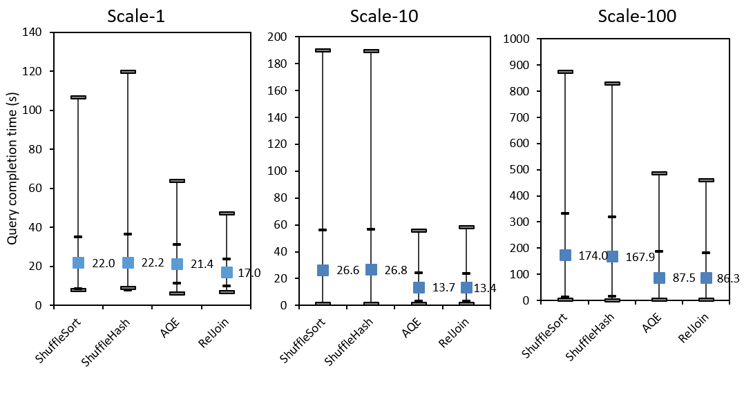
Figure 4: The average completion time of TPC-DS queries of various strategies in benchmarks of different scales

RelJoin reduces the average and maximum query completion time significantly. RelJoin also reduces the standard deviation of the query time among different queries. The query completion time results of the different strategies for benchmarks of different scales are shown in Fig. 4. The square blocks are the average time results, the higher and lower rectangle bars at both ends are the maximum and minimum time results, and the smaller line bars are the average time $\pm$ standard deviation results. Compared to ShuffleSort, ShuffleHash, and AQE, RelJoin reduces the average query time by 22.7%, 23.6%, and 20.8%, respectively, in the scale-1 benchmark; by 49.3%, 49.8%, and 2.0%, respectively, in the scale-10 benchmark; and by 50.4%, 48.6%, and 1.3%, respectively, in the scale-100 benchmark. In addition, both AQE and RelJoin significantly decrease the maximum query time by allowing the broadcast hash join method. Compared to ShuffleSort, ShuffleHash, and AQE, RelJoin reduces the maximum query time by 55.6%, 60.5%, and 26.1% in the scale-1 benchmark and by 47.5%, 44.6%, and 5.5% in the scale-100 benchmark, respectively. RelJoin also has a lower standard deviation of query time than the other strategies, indicating that the query performance is less dispersed in RelJoin.

We attributed the reduction in the average and maximum query time by AQE and RelJoin compared with ShuffleSort and ShuffleHash to the selection of the broadcast hash method when it is considered to be better than the other distributed join methods: the shuffle sort and shuffle hash methods. Broadcasting a (relatively) small dataset helps to decrease the network communication workload by eliminating the need to shuffle the other large dataset. For example, query q72 in the scale-1 benchmark consists of ten logical joins, nine of which have massive left datasets and small right datasets with a maximum size of 1.4 MB. The completion time of query q72, which is the maximum in both ShuffleSort (106 s) and ShuffleHash (119 s), is reduced to 38 s for AQE and 26 s for RelJoin. The broadcast hash join decreases the network traffic and the query time significantly.

We further examine the optimization of another query in the scale-1 benchmark, q39b, to determine how the cost model of RelJoin makes a distributed join method selection. The completion times of query q39b are 42 and 35 s in ShuffleSort and ShuffleHash, respectively, but are reduced to 16 and 15 s in BroadcastShuffle and RelJoin, respectively. Query q39b has seven logical joins and RelJoin selects the broadcast hash method for six joins, in one of which the left and right datasets are approximately 40 and 0.13 MB, respectively. According to Equations 4 and 8, the costs of the broadcast hash join and the shuffle sort join are 45.2 MB and 78.4 MB, respectively. By selecting the broadcast hash method, RelJoin outperform ShuffleSort and ShuffleHash in the cases of joins with a relatively small dataset.

However, the absolute size criterion in AQE may abuse the broadcast hash join method selection. We examine the join method selection results for all query plans in the scale-1 benchmark. AQE and RelJoin make 600 and 540 broadcast hash join selections, respectively, out of the 629 joins. More broadcast hash joins than the appropriate results in AQE perform worse than RelJoin in this benchmark. As the dataset scale increases, more datasets exceed the threshold for AQE to select the broadcast hash join method. AQE decreases the number of broadcast hash join method selections, behaving more like RelJoin and approaching its query performance. Despite this, RelJoin retains the ability to select the broadcast hash join method in larger-scale benchmarks to reduce the query time for queries in which both joining datasets have large absolute sizes, but one is relatively smaller than the other. This explains why AQE achieves similar average query time results to RelJoin, but RelJoin can still decrease the maximum query time by 5.5% in the scale-100 benchmark.

The distribution of the query completion time in the scale-1 benchmark in Fig. 5 shows how RelJoin improves the average query time in the bigger picture. The peak of RelJoin in the query time distribution is to the left of those of the other strategies. The numbers of queries that are completed within 15 s by ShuffleSort, ShuffleHash, AQE, and RelJoin are 25, 24, 5, and 41, respectively. The numbers within 20 s are 59, 61, 35, and 69, respectively. RelJoin decreases the completion time for some queries known as outliers, as well as for a wide set of queries. However, AQE has a fatter tail, indicating that it has more queries with a longer completion time. This is because it may select the broadcast hash join method when broadcasting introduces no performance benefit or, worse, costs more than shuffling. This is discussed in more details in Section 5.4.

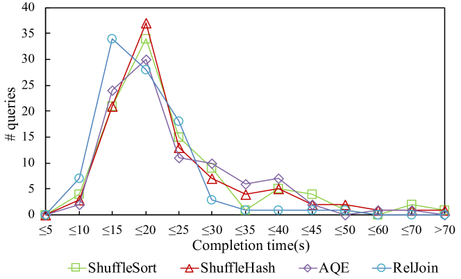
Figure 5: The distribution of query completion time of various strategies in the scale-1 benchmark

5.3 Optimization accuracy

When comparing a set of selection strategies, if the strategy that results in the lowest query completion time is viewed as optimal for a query, the query-wise optimization accuracy of RelJoin is as high as 63.9%, which is much higher than that of the other strategies. Table 4 presents the number of queries for which each strategy is optimal and the corresponding optimization accuracy (percentage of optimized queries) for benchmarks of different scales. Without RelJoin in the comparison, the optimization accuracy results of ShuffleSort and ShuffleHash are close to one another, whereas those of AQE are higher. A comparison of all four strategies shows that RelJoin makes the best selection for 62 of the 97 queries, 45 of the 93 queries, and 36 of the 90 queries in the scale-1, scale-10, and scale-100 benchmarks, respectively. As the queries in TPC-DS are complex queries with multiple joins, RelJoin exhibits better results by selecting distributed join methods with the lowest cost for each logical join and generating the optimal combination of a sequence of join methods. This is the major optimization idea of RelJoin  which distinguishes it from other strategies, and it outperforms them in most queries. As discussed in Section 5.2, with larger datasets in the TPC-DS benchmark, AQE narrows the performance gap with RelJoin by selecting fewer broadcast hash joins and behaves more like RelJoin. Consequently, the optimization accuracies of these two strategies are similar for the scale-100 benchmark.

Table 4: The number of queries that a strategy achieves the least query time and the corresponding optimization accuracy in benchmarks of different scales. The results with RelJoin excluded (First-3) and included (All) in the comparison are shown. The results are represented as #number(%accuracy).

	Scale-1		Scale-10		Scale-100
Strategy	First-3	All	First-3	All	First-3	All
ShuffleSort	33(34.0)	14(14.4)	12(12.9)	12(12.9)	2(2.22)	2(2.22)
ShuffleHash	28(28.9)	9(9.3)	7(7.5)	7(7.5)	10(11.1)	10(11.1)
AQE	36(37.1)	12(12.4)	74(79.6)	32(34.4)	78(86.7)	42(46.7)
RelJoin	-	62(63.9)	-	45(45.2)	-	36(40.0)
Total	97(100)	97(100)	93(100)	93(100)	90(100)	90(100)

Different local join methods that are applied by distributed joins are minor factors influencing the query performance. Fig. 4, Fig.5 , and Table 4 all indicate that the shuffle sort and shuffle hash methods have very similar results in terms of the average query time, query time distribution, and optimization accuracy.

5.4 Relative size vs. absolute size: criterion for broadcasting

Hereafter, we use the results of the scale-1 benchmark to explore additional properties and mechanisms of RelJoin.

We further claim that the relative size of the two joining datasets used by RelJoin is a better criterion than the absolute size when using the broadcast hash method. AQE and RelJoin are similar strategies that allow broadcast hash joins when they judge a dataset to be sufficiently small for broadcasting. They differ in the criterion of determining sufficiently small datasets. The former uses the user-configured absolute size, whereas the latter uses the relative size considering the distributed join parallelism and network cost weight.

We delve deeper into the query plans and join method selection results for these two strategies to verify our claim. As our focus is the performance difference between broadcasting and shuffling, and the shuffle sort and shuffle hash methods have similar performances, we consider these shuffle methods as the same method. We sort out the distributed join methods and corresponding statistics, where one strategy selects the broadcast hash method and the other selects a shuffle method. For a query in which the strategies make different join method selections, the cost difference based on our cost model and the query completion time difference are recorded. Among the 629 selections in the scale-1 benchmark, these two strategies make different selections in 66 cases, in 63 of which RelJoin selects shuffle methods and AQE selects broadcast hash methods, and in three of which they do so in reverse. The benchmark cost difference is 5834.2 MB, and the benchmark completion time difference is 419.9 s which is 20.8% of the AQE benchmark completion time, as indicated in Table 5. With everything else remaining the same, the performance improvement is attributed to the join method selection difference. Each different method selection made by RelJoin contributes to a cost reduction of 88.4 MB and a query completion time reduction of 6.4 s.

Table 5: Comparing RelJoin with AQE, the statistics of (1) the number of different and total join method selections, (2) the resulted cost difference, (3) the resulted query time reduction, (4) the cost difference per number of different join method selections, (5) the query time difference per number of different join method selections, (6) the percentage of different join method selections to the total number of joins, (7) the percentage of time reduction, and (8) the performance sensitivity to selections (PSTS).

Statistics	Value
(1) #JoinDiff (#Join)	66 (629)
(2) CostDiff	5834.2 MB
(3) TimeDiff	419.9s
(4) CostDiff / #JoinDiff	88.4 MB
(5) TimeDiff / #JoinDiff	6.4s
(6) %JoinDiff	10.5%
(7) %TimeDiff	20.8%
(8) %TimeDiff / %JoinDiff (PSTS)	1.98

However, the above metrics rely on benchmark-specific properties, such as the size of the dataset and number of queries, and are not comparable across benchmarks to reflect the optimization effectiveness of different strategies directly. We propose the term Performance Sensitivity To Selections (PSTS) as a metric to measure the query optimization effectiveness of a join method selection strategy. The PSTS is calculated as the percentage of the time difference divided by the percentage of the join method selection difference, which indicates the extent to which the query completion time is affected by the optimization result of a selection strategy with AQE as the baseline. A PSTS of 1 indicates that a 1% difference in the number of join methods selected by a selection strategy contributes to a 1% reduction in the benchmark completion time. In general, a higher PSTS indicates that the query optimization is more effective . When the PSTS is close to 0 or even negative, the optimization of a selection strategy is ineffective or even negatively affects the query performance. In the TPC-DS case, the PSTS of RelJoin is 1.98, which suggests that RelJoin effectively optimizes the query plan compared with AQE. As a reference, the PSTSs of ShuffleSort and ShuffleHash in TPC-DS are $-0.03$ and $-0.04$, respectively, which indicates that they have slightly negative optimization effects compared with AQE. The results of the PSTS do not include benchmark-specific properties and are comparable across benchmarks for optimization effectiveness.

RelJoin outperforms AQE mainly by not using the broadcast hash method when one dataset is not sufficiently smaller than the other in a join. Among the 66 cases of inconsistent join method selections, RelJoin resolves that shuffle methods are better selections in 63. RelJoin selects the broadcast hash method only when the larger dataset is 39 times as large as the smaller dataset ($k_{0}=39$). However, AQE selects the broadcast hash method as 1.10 MB is smaller than the broadcast size threshold (10 MB). When considering the selection of a broadcast hash method, the relative size criterion used by RelJoin is better than the absolute size criterion used by AQE.

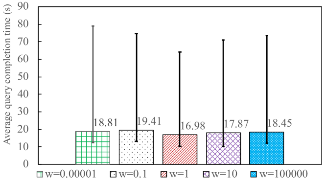
Figure 6: The average query completion time of RelJoin with different $w$ values in the scale-1 benchmark

5.5 The impact of $w$

We explore the impact of different values of $w$, which is the relative weight of the network cost on the computing cost. Fig. 6 shows that RelJoin has similar average, maximum, and minimum query times in the scale-1 TPC-DS benchmark with $w$ at different scales.

Different configurations of $w$ have a relatively higher impact on the maximum query time than on the average query time. The trend of the maximum query time exhibits an obvious “V” shape, with $w=1$ at the bottom of the valley, which is 21.4% and 14.4% lower than that when $w=0.00001$ and $w=100,000$, respectively. This suggests that the optimal configuration of $w$ is approximately 1 in our testbed. When $w$ is substantially larger than 1 (for instance, as large as 100,000), the overall cost is determined entirely by the network cost. The average query time of 18.45 s is slightly larger than that when $w=1$, but is still more than 16% smaller than the query time of the ShuffleSort, ShuffleHash, and AQE strategies (Fig. 4). We also test the case of $w=0.1$, where the overall cost is mainly determined by the local computing cost, which may occur in the fast network, e.g., the zero-copy networking of the Remote Direct Memory Access (RDMA) technology, and slow memory scenarios. Owing to the build phase, which builds a hash map for the entire replicate dataset in each task, the local computing cost of the broadcast hash method is higher than those of the shuffle methods. RelJoin behaves more similarly to ShuffleSort and ShuffleHash, and tends to select shuffle methods when shuffling network traffic is not significant compared with broadcasting. The average and maximum query times both increase by approximately 15% compared to the case of $w=1$. Weakening or overemphasizing the network cost slightly degrades the query performance. Regarding the “V” trend, tuning the optimal $w$ is similar to a convex problem, where users can start with an empirically near-optimal value first, such as $w=1$, and attempt values leading to the downtrend.

We have highlighted some important evaluation results. First, compared with AQE, RelJoin reduces the average and maximum query completion times by 20.8% and 26.1%, respectively. Second, RelJoin achieves the best completion time for 62 of the 97 queries, which is five times as high as that of AQE. Third, with AQE as the baseline, the PSTS of RelJoin is 1.98 for the scale-1 benchmark, which indicates that 1% of the join selection optimization contributes to a 1.98% reduction in the query completion time. Fourth, tuning the hyperparameter $w$ is straightforward. Setting $w$ either too large or too small will slightly degrade the performance, but it still performs better than AQE.

6 Related work

Cost-based join query optimization has long been an important topic in database query optimization. It often encounters the combination explosion problem, resulting in a locally optimal plan. Oracle [2, 10, 16] uses a set of rules to generate many combinations of physical alternatives for a sequence of logical operations, following which it uses cost-based optimization to search for the optimal query plan with the lowest cost, which can easily run into potential combination explosion problems. To address this problem, Oracle performs a quasi-random walk in the search, which achieves a local minimum cost at every step. RelJoin also performs a quasi-random walk to select the least-cost distributed join method for a sequence of logical join operations in the query plan. However, for the optimization problem of distributed join method selection, because the cost and selection of a distributed join method for a logical join are independent of those for other logical joins in the query plan, the best join method for each logical join leads to the globally optimal physical plan.

Most cost-based join optimizations [14, 20, 28, 34, 39] work on cost-efficient methods to achieve the optimal join order, by using heuristic, randomized, or genetic algorithms. The accuracy of dataset statistics is crucial for determining the optimal join order. Some studies have obtained statistics by sampling [24] or adapted statistics based on the runtime statistics from every execution stage [11, 13]. In recent years, many machine-learning-based models [32, 35, 40, 42] have been developed to estimate the dataset cardinality and to rewrite the query plan for the optimal join order. RelJoin can work together with join order optimization strategies to achieve the best performance. It uses adaptive runtime statistics to select the best physical join method for logical joins that are already in the optimal join order.

Many cost models for join methods focus on the local join cost for query optimization and do not precisely incorporate the network cost of the distributed environment. Some models [6, 19, 26, 27] analyze the complexity of the algorithm implementation of the hash join and sort join, and compare their costs based on the use of CPU, memory, and disk I/O in different computing phases. Other methods [25, 38] predict the query time of joins by calibrating the cardinality workloads, measuring the speeds of local computing resources, and analyzing the memory I/O access patterns. Some methods [8, 9] model the partitioning cost of shuffle-like distributed joins via RDMA transfers in the data exchange phase, and mainly compare the cost differences in the local join phase, but not the network costs of different data exchange methods. RelJoin explores and compares the broadcast and shuffle costs in the data exchange phase of various distribution methods and emphasizes the network cost in the cost model.

Table 6: A summary of the comparison of the characteristics of RelJoin with other distributed join cost models

	[25]	[9]	[17]	[5]	[22]	[29]	[30]	Ours
Workload-based	$\checkmark$	$\checkmark$	$\checkmark$		$\checkmark$	$\checkmark$	$\checkmark$	$\checkmark$
Time-based				$\checkmark$
Rely on data volume	$\checkmark$	$\checkmark$	$\checkmark$	$\checkmark$	$\checkmark$	$\checkmark$	$\checkmark$	$\checkmark$
Rely on access patterns	$\checkmark$
Rely on I/O throughput		$\checkmark$	$\checkmark$	$\checkmark$		$\checkmark$	$\checkmark$
Require abundant tuning					$\checkmark$
Consider resource allocation				$\checkmark$			$\checkmark$	$\checkmark$
Consider data relations		$\checkmark$	$\checkmark$	$\checkmark$		$\checkmark$	$\checkmark$	$\checkmark$
Robust with data skew			$\checkmark$			$\checkmark$		$\checkmark$

Many cost models [5, 17, 22, 29, 30] also consider the network cost of distributed join methods; however, they are highly dependent on the hardware access patterns whose performance values are difficult to determine on scalable platforms or involve abundant hyperparameters that are specific to the complex distributed environment, leading to potential practical problems. For example, the cost model proposed by Baldacci and Golfarelli [5] requires accurate measurement of the disk read/write throughput between processes and the network throughput between nodes in the same rack or across racks. The cost model proposed by Lian and Zhang [22] requires the tuning of several hyperparameters matrices based on the empirical correlative cost of all physical plan candidates. There are also concerns regarding data skew. Phan et al. [30] modeled the costs of various distributed join methods but provided no evidence of robustness in data skew cases. Some cost models [17, 29] address the data skew problem by incorporating the skewness assumption into the problem setting. However, the above cost models fail to realize the importance of the relative size of the joining datasets in determining the join costs. RelJoin relates the cluster workload to the relative sizes of the joining datasets and has only one hyperparameter, which does not sensitively affect the query performance in modern network environments. Moreover, our analysis of the impact of data skew showed that the cluster workload modeling method makes RelJoin robust even when data skew exists. Table 6 compares the characteristics of RelJoin with those of other distributed join models.

Other optimizations of distributed joins [15, 23, 31] include considering the relationship and locality of the data of multiple join operations, such that data can be joined locally with less network traffic during a sequence of joins. These optimizations can help to refine the data exchange phase cost and performance in RelJoin.

7 Conclusions and future work

In this study, we have developed and compared the cost models of various distributed join methods that precisely estimate network workloads using adaptive runtime statistics. We integrated the distributed join cost model into RelJoin, which is an efficient query optimization strategy that selects the best distributed join methods for logical joins in the query plan. The evaluation results for the TPC-DS benchmark show that RelJoin is optimal for most queries and significantly improves the query completion time.

In the future, we will work on learning-based cost models to connect workloads to the query completion time such that minimizing the query cost is directly related to the target of minimizing the query completion time. Moreover, the cost-based distributed join method selection strategy in query plan optimization motivates us to discover more potential variants of distributed join implementations that can optimize the join query performance in specific cluster environments with specific query workloads.

References

- [1] Tpc-ds, . URL: https://www.tpc.org/tpcds/.
- Ahmed et al. [2006] Ahmed, R., Lee, A., Witkowski, A., Das, D., Su, H., Zait, M., Cruanes, T., 2006. Cost-based query transformation in oracle, in: VLDB, pp. 1026–1036.
- Albutiu et al. [2012] Albutiu, M.C., Kemper, A., Neumann, T., 2012. Massively parallel sort-merge joins in main memory multi-core database systems. Proceedings of the VLDB Endowment 5.
- Armbrust et al. [2015] Armbrust, M., Xin, R.S., Lian, C., Huai, Y., Liu, D., Bradley, J.K., Meng, X., Kaftan, T., Franklin, M.J., Ghodsi, A., et al., 2015. Spark sql: Relational data processing in spark, in: Proceedings of the 2015 ACM SIGMOD international conference on management of data, pp. 1383–1394.
- Baldacci and Golfarelli [2018] Baldacci, L., Golfarelli, M., 2018. A cost model for spark sql. IEEE Transactions on Knowledge and Data Engineering 31, 819–832.
- Balkesen et al. [2013] Balkesen, Ç., Alonso, G., Teubner, J., Özsu, M.T., 2013. Multi-core, main-memory joins: Sort vs. hash revisited. Proceedings of the VLDB Endowment 7, 85–96.
- Balkesen et al. [2014] Balkesen, Ç., Teubner, J., Alonso, G., Özsu, M.T., 2014. Main-memory hash joins on modern processor architectures. IEEE Transactions on Knowledge and Data Engineering 27, 1754–1766.
- Barthels et al. [2015] Barthels, C., Loesing, S., Alonso, G., Kossmann, D., 2015. Rack-scale in-memory join processing using rdma, in: Proceedings of the 2015 ACM SIGMOD International Conference on Management of Data, pp. 1463–1475.
- Barthels et al. [2017] Barthels, C., Müller, I., Schneider, T., Alonso, G., Hoefler, T., 2017. Distributed join algorithms on thousands of cores. Proceedings of the VLDB Endowment 10, 517–528.
- Bellamkonda et al. [2009] Bellamkonda, S., Ahmed, R., Witkowski, A., Amor, A., Zait, M., Lin, C.C., 2009. Enhanced subquery optimizations in oracle. Proceedings of the VLDB Endowment 2, 1366–1377.
- Bellamkonda et al. [2013] Bellamkonda, S., Hua-Gang, L., Unmesh, J., Yali, Z., Vince, L., Thierry, C., 2013. Adaptive and big data scale parallel execution in oracle. Proceedings of the VLDB Endowment 6, 1102–1113.
- Blanas et al. [2011] Blanas, S., Li, Y., Patel, J.M., 2011. Design and evaluation of main memory hash join algorithms for multi-core cpus, in: Proceedings of the 2011 ACM SIGMOD International Conference on Management of data, pp. 37–48.
- Chakkappen et al. [2017] Chakkappen, S., Budalakoti, S., Krishnamachari, R., Valluri, S.R., Wood, A., Zait, M., 2017. Adaptive statistics in oracle 12c. Proceedings of the VLDB Endowment 10, 1813–1824.
- Chen et al. [2009] Chen, Y., Cole, R.L., McKenna, W.J., Perfilov, S., Sinha, A., Szedenits Jr, E., 2009. Partial join order optimization in the paraccel analytic database, in: Proceedings of the 2009 ACM SIGMOD International Conference on Management of data, pp. 905–908.
- Cheng et al. [2017] Cheng, L., Kotoulas, S., Ward, T.E., Theodoropoulos, G., 2017. Improving the robustness and performance of parallel joins over distributed systems. Journal of Parallel and Distributed Computing 109, 310–323.
- Das et al. [2015] Das, D., Yan, J., Zait, M., Valluri, S.R., Vyas, N., Krishnamachari, R., Gaharwar, P., Kamp, J., Mukherjee, N., 2015. Query optimization in oracle 12c database in-memory. Proceedings of the VLDB Endowment 8, 1770–1781.
- García-García et al. [2023] García-García, F., Corral, A., Iribarne, L., Vassilakopoulos, M., 2023. Efficient distributed algorithms for distance join queries in spark-based spatial analytics systems. International Journal of General Systems 52, 206–250.
- Kaseb et al. [2021] Kaseb, M.R., Haytamy, S.S., badry, R.M., 2021. Distributed query optimization strategies for cloud environment. Journal of Data, Information and Management 3, 271–279.
- Kim et al. [2009] Kim, C., Kaldewey, T., Lee, V.W., Sedlar, E., Nguyen, A.D., Satish, N., Chhugani, J., Di Blas, A., Dubey, P., 2009. Sort vs. hash revisited: Fast join implementation on modern multi-core cpus. Proceedings of the VLDB Endowment 2, 1378–1389.
- Leis et al. [2015] Leis, V., Gubichev, A., Mirchev, A., Boncz, P., Kemper, A., Neumann, T., 2015. How good are query optimizers, really? Proceedings of the VLDB Endowment 9, 204–215.
- Li et al. [2018] Li, Y., Li, M., Ding, L., Interlandi, M., 2018. Rios: Runtime integrated optimizer for spark, in: Proceedings of the ACM Symposium on Cloud Computing, pp. 275–287.
- Lian and Zhang [2018] Lian, X., Zhang, T., 2018. The optimization of cost-model for join operator on spark sql platform, in: MATEC Web of Conferences, EDP Sciences. p. 01015.
- Liang et al. [2017] Liang, F., Lau, F.C., Cui, H., Wang, C.L., 2017. Confluence: speeding up iterative distributed operations by key-dependency-aware partitioning. IEEE Transactions on Parallel and Distributed Systems 29, 351–364.
- Lipton et al. [1990] Lipton, R.J., Naughton, J.F., Schneider, D.A., 1990. Practical selectivity estimation through adaptive sampling, in: Proceedings of the 1990 ACM SIGMOD international conference on Management of data, pp. 1–11.
- Liu and Blanas [2015] Liu, F., Blanas, S., 2015. Forecasting the cost of processing multi-join queries via hashing for main-memory databases, in: Proceedings of the Sixth ACM Symposium on Cloud Computing, pp. 153–166.
- Manegold et al. [2002a] Manegold, S., Boncz, P., Kersten, M., 2002a. Optimizing main-memory join on modern hardware. IEEE Transactions on Knowledge and Data Engineering 14, 709–730.
- Manegold et al. [2002b] Manegold, S., Boncz, P., Kersten, M.L., 2002b. Generic database cost models for hierarchical memory systems, in: VLDB’02: Proceedings of the 28th International Conference on Very Large Databases, Elsevier. pp. 191–202.
- Mei and Madden [2009] Mei, Y., Madden, S., 2009. Zstream: a cost-based query processor for adaptively detecting composite events, in: Proceedings of the 2009 ACM SIGMOD International Conference on Management of data, pp. 193–206.
- Phan et al. [2022] Phan, A.C., Phan, T.C., Cao, H.P., Trieu, T.N., 2022. Comparative analysis of skew-join strategies for large-scale datasets with mapreduce and spark. Applied Sciences 12, 6554.
- Phan et al. [2021] Phan, A.C., Phan, T.C., Trieu, T.N., Tran, T.T.Q., 2021. A theoretical and experimental comparison of large-scale join algorithms in spark. SN Computer Science 2, 352.
- Polychroniou et al. [2014] Polychroniou, O., Sen, R., Ross, K.A., 2014. Track join: distributed joins with minimal network traffic, in: Proceedings of the 2014 ACM SIGMOD international conference on Management of data, pp. 1483–1494.
- Robinson et al. [2014] Robinson, N., McIlraith, S.A., Toman, D., 2014. Cost-based query optimization via ai planning, in: Proceedings of the Twenty-Eighth AAAI Conference on Artificial Intelligence, pp. 2344–2351.
- Sharma et al. [2019] Sharma, M., Singh, G., Singh, R., 2019. A review of different cost-based distributed query optimizers. Progress in Artificial Intelligence 8, 45–62.
- Steinbrunn et al. [1997] Steinbrunn, M., Moerkotte, G., Kemper, A., 1997. Heuristic and randomized optimization for the join ordering problem. The VLDB Journal 6, 191–208.
- Sun and Li [2019] Sun, J., Li, G., 2019. An end-to-end learning-based cost estimator. Proceedings of the VLDB Endowment 13.
- Thusoo et al. [2009] Thusoo, A., Sarma, J.S., Jain, N., Shao, Z., Chakka, P., Anthony, S., Liu, H., Wyckoff, P., Murthy, R., 2009. Hive: a warehousing solution over a map-reduce framework. Proceedings of the VLDB Endowment 2, 1626–1629.
- Vavilapalli et al. [2013] Vavilapalli, V.K., Murthy, A.C., Douglas, C., Agarwal, S., Konar, M., Evans, R., Graves, T., Lowe, J., Shah, H., Seth, S., et al., 2013. Apache hadoop yarn: Yet another resource negotiator, in: Proceedings of the 4th annual Symposium on Cloud Computing, pp. 1–16.
- Wu et al. [2013] Wu, W., Chi, Y., Zhu, S., Tatemura, J., Hacigümüs, H., Naughton, J.F., 2013. Predicting query execution time: Are optimizer cost models really unusable?, in: 2013 IEEE 29th International Conference on Data Engineering (ICDE), IEEE. pp. 1081–1092.
- Wu et al. [2003] Wu, Y., Patel, J.M., Jagadish, H., 2003. Structural join order selection for xml query optimization, in: Proceedings 19th International Conference on Data Engineering, IEEE. pp. 443–454.
- Yang et al. [2019] Yang, Z., Liang, E., Kamsetty, A., Wu, C., Duan, Y., Chen, X., Abbeel, P., Hellerstein, J.M., Krishnan, S., Stoica, I., 2019. Deep unsupervised cardinality estimation. Proceedings of the VLDB Endowment 13.
- Yin et al. [2015] Yin, S., Hameurlain, A., Morvan, F., 2015. Robust query optimization methods with respect to estimation errors: A survey. ACM Sigmod Record 44, 25–36.
- Zhou et al. [2021] Zhou, X., Li, G., Chai, C., Feng, J., 2021. A learned query rewrite system using monte carlo tree search. Proceedings of the VLDB Endowment 15, 46–58.