Identification of odd-frequency superconducting pairing in Josephson junctions

Abstract

Choosing the right spin polarization of electron enables its local injection into the helical edge state with a well-defined momentum direction, despite the uncertainty principle, owing to spin-momentum locking. This fact facilitates a direct identification of odd-frequency pairing through parity measurement (under frequency reversal) of the anomalous Green’s function in a setup comprising multi-terminal Josephson junction on the helical edge state of a 2D topological insulator.

Introduction: In a conventional superconductor, electrons form Cooper pairs due to a weak attraction mediated via lattice vibrations[1]. The pairing function between the two electrons within a Cooper pair can be classified into different symmetry classes by means of four permutation operators with respect to spin ($S$), relative coordinate ($P^{*}$), orbital index ($O$), and time coordinate ($T^{*}$), all of which can only have eigenvalues $\pm 1$. Generally, BCS theory of uniform superconductor ($\expectationvalue{O}=1$) is instantaneous in time ($\expectationvalue{T^{*}}=1$). This leaves two choices for the combinations of eigenvalues of the operators $S$ and $P^{*}$ to satisfy the Berezinskii condition[2] $SP^{*}OT^{*}=-1$ for the pairing function, i.e., $\{\expectationvalue{S},\expectationvalue{P^{*}}\}=\{-1,1\},\{1,-1\}$. These correspond to spin-singlet even-parity (e.g. $s$-wave) and spin-triplet odd-parity[3] (e.g. $p$-wave) symmetries, respectively. If one removes the constraint of instantaneous pairing, the possibility of temporal (non-local in time) Cooper pairing becomes feasible, and both $\expectationvalue{T^{*}}=\pm 1$ can be possible, depending on whether the pairing function is symmetric or anti-symmetric under the permutation of relative time coordinates of the electrons forming the Cooper pair. Temporally symmetric pairing ($\expectationvalue{T^{*}}=1$) does not give rise to any new symmetry classes other than those already described by BCS theory and is generally known as even-frequency (even-$\omega$) pairing. However, temporally anti-symmetric pairing ($\expectationvalue{T^{*}}=-1$), which is known as odd-frequency (odd-$\omega$) pairing[4, 5, 6], opens up possibilities of two new symmetry classes (assuming $\expectationvalue{O}=1$) that cannot be described by BCS theory, namely, spin-singlet odd-parity ($\{\expectationvalue{S},\expectationvalue{P^{*}}\}=\{-1,-1\}$) and spin-triplet even-parity ($\{\expectationvalue{S},\expectationvalue{P^{*}}\}=\{1,1\}$) pairings, consistent with Berezinskii condition. It can also be shown that this odd-$\omega$ (even-$\omega$) pairing is also odd (even) under the sign change of energy[4], which gives the advantage of observing the behavior of this pairing in the energy domain rather than in the temporal domain.

On a historical note, the concept of odd-$\omega$ spin-triplet pairing traces back to Berezinskii’s 1974 proposal in ³He[2] and predictions in disordered systems[7, 8]. Balatsky and Abrahams later indicated the presence of odd-$\omega$ spin-singlet pairing in time-reversal and parity symmetry broken superconductors[9]. Subsequently, the odd-$\omega$ pairing was explored within the framework of a two-channel Kondo system[10], the 1D $t-J-h$ model[11], the 2D Hubbard model[12] and heavy fermion compounds[13]. The bulk odd-$\omega$ pairing has been indirectly hinted theoretically through the Majorana scanning tunneling microscope[14] and also experimentally using the Kerr effect[15, 16], and the paramagnetic Meissner effect[17, 18, 19, 20, 21]. Further, the evidence of bulk odd-$\omega$ pairing due to magnetic impurities has emerged in $s$-wave superconductors[22, 23]. In Ref. [24], a measurement tool was introduced for directly detecting odd-$\omega$ pairing in bulk systems using time- and angle-resolved photoelectron fluctuation spectroscopy. However, this method requires advanced technology beyond the current capabilities of facilities. More recently, in Ref. [25], authors proposed a detection scheme to directly identify odd-$\omega$ pairing in bulk systems using the quasiparticle interference method in the presence of an external magnetic field. Initially, odd-$\omega$ pairing was regarded as an inherent bulk phenomenon[2, 9, 26] but was subsequently acknowledged to manifest in heterojunctions[27, 28, 29, 30, 31, 32, 33, 34, 35, 36, 37, 38, 39, 40, 41, 42, 43, 44, 45, 46, 47, 48, 49, 50, 51, 52, 53] and in the systems under the influence of time-dependent fields[54, 55]. Certain theoretical studies have indirectly identified odd-$\omega$ pairing in heterostructures. For instance, this was achieved through phase-tunable electron transport in topological Josephson junctions (JJ)[56], examining Josephson current characteristics on the surface of Weyl nodal loop semimetals[57], and analyzing current noise in JJ[58]. Experimental evidence of odd-$\omega$ pairing in heterostructures emerged through measurements of long-range supercurrents in magnetic JJ[59, 60]. These two experiments utilize a ferromagnetic material to create an odd-$\omega$ pairing effect, which is subsequently identified by measuring long-range superconducting pairing. In contrast, this letter investigates a configuration that inherently supports odd-$\omega$ pairing without the need for any ferromagnet/superconductor junction. Topological JJ at the edge of a two-dimensional (2D) quantum-spin-Hall insulator (QSHI) serves this purpose.

We demonstrate that it is possible to read off all the independent, spatially non-local Green’s functions by measuring differential conductance between weakly tunneled coupled spin-polarized leads placed at the junction. This advantage is made possible due to the interplay between spin-momentum locking of helical edge states (HES) and spin-polarization of the probes. This advantage hinges upon the fact that by using spin-polarized probes, one can inject electrons into the helical edge with well-defined position and momentum simultaneously, which, in general, is prohibited due to uncertainty principle[61]. To elaborate further, a spin-$\uparrow$ electron injected at position $x$ in the helical edge can only tunnel into the right moving edge mode owing to spin-momentum locking. Keeping the spin-polarization axes of the tunneling probes aligned parallel or anti-parallel to the spin-quantization axis of HES, we study the difference between non-local differential conductance from the left probe to right probe $\kappa^{21}_{s\bar{s}}(V,0)$ and from right probe to left probe $\kappa^{12}_{\bar{s}s}(0,V)$ i.e.

$$\mathcal{A}(\kappa_{s\bar{s}}^{21}) =\kappa^{21}_{s\bar{s}}(V_{1}=V,V_{2}=0)-\kappa^{12}_{\bar{s}s}(V_{1}=0,V_{2}=V)$$

$$=\left[\dfrac{dI_{s\bar{s}}^{21}}{dV}\right]_{(V_{1}=V,V_{2}=0)}-\left[\dfrac{dI_{\bar{s}s}^{12}}{dV}\right]_{(V_{1}=0,V_{2}=V)}$$ (1)

where $\{s,\bar{s}\}\in\{\uparrow,\downarrow\}$ with $s\neq\bar{s}$, and $V_{1}(V_{2})$ denotes the applied voltage at the left (right) tunneling probe. It can be shown that this quantity $\mathcal{A}(\kappa^{21}_{s\bar{s}})$ can be written as a product of odd-$\omega$ and even-$\omega$ pairing amplitudes and hence should be odd with respect to incident energy, i.e., $eV$. We show that this difference stems from the same origin as that of the odd-$\omega$ part of the non-local differential conductance, which can be accessed via bias reversal i.e. $\mathcal{B}(\kappa^{21}_{s\bar{s}})=\kappa^{21}_{s\bar{s}}(V,0)-\kappa^{21}_{s\bar{s}}(-V,0)$. This fact leads to

$$\mathcal{A}(\kappa_{s\bar{s}}^{21})=\mathcal{B}(\kappa^{21}_{s\bar{s}}).$$ (2)

From an experimental perspective, measuring the anti-symmetric behavior of each of these independent quantities and their equality confirms the existence of odd-$\omega$ pairing.

Model and its motivation: The system, we are interested in, is a JJ of length $L$ ($0\leq x\leq L$), realized in a helical edge state (HES) of a 2D QSHI[62, 63, 64, 65] (1D Dirac fermions) which is proximitized to a conventional $s$-wave superconductor (FIG. 1). The Bogoliubov-de Gennes (BdG) Hamiltonian characterizing such junctions can be written as[66, 67] $H_{J}=\int_{-\infty}^{\infty}dx\,\Psi^{\dagger}\mathcal{H}_{J}\Psi$ where $\Psi=(\psi_{\uparrow},\psi_{\downarrow},\psi_{\downarrow}^{\dagger},-\psi_{\uparrow}^{\dagger})^{T}$ is the Nambu basis and

$$\mathcal{H}_{J}=-i\hbar v_{F}\partial_{x}\tau_{z}\sigma_{z}-\mu\tau_{z}+{\Delta}(x)(\cos{\varphi_{r}}\tau_{x}-\sin{\varphi_{r}}\tau_{y})\,.$$ (3)

Here, $\sigma_{i}$ and $\tau_{i}$ are the Pauli matrices acting respectively on the spin basis and particle-hole basis, $\mu$ is the chemical potential of the HES, and $v_{F}$ is the corresponding Fermi velocity. The spin-quantization axis of the HES is considered to be along $z$-direction[66, 67]. The superconducting pairing magnitude $|\Delta(x)|=\Delta_{0}[\Theta(-x)+\Theta(x-L)]$ is assumed to be the same in both the superconductors. However, the superconducting phases $\varphi_{r}$’s ($r=1,2$ for left and right superconductors respectively), in general, are considered to be different, and $\varphi_{21}=\varphi_{2}-\varphi_{1}$ represents the phase difference.

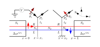
Figure 1: Josephson junction at the edge of a 2D QSHI with two spin-polarized tunneling probes at $x=x_{1}$ and $x=x_{2}$. Up and down arrows represent the spin polarization direction of helical edge states, with the left tunneling probe ($P_{1}$) at an angle $\theta_{1}$ to the $z$-axis and the right tunneling probe ($P_{2}$) at an angle $\theta_{2}$. A bias voltage $V$ is applied to $P_{1}$ while $P_{2}$ is grounded.

Two spin-polarized tunneling probes[68] ($P_{1}$ and $P_{2}$) with spin-polarization axes oriented respectively along $\hat{n}_{1}$ and $\hat{n}_{2}$, at angles $\theta_{1}$ and $\theta_{2}$ with respect to the spin-quantization axis of the HES (say, in the $z-x$ plane), are introduced at positions $x=x_{1}$ and $x=x_{2}$ respectively within the junction region ($0<x_{1}<x_{2}<L$). To keep the algebra simple while retaining the essential physical inputs, we model the probes as a spin-polarized 1D mode. The second quantized Hamiltonians of these probes can be expressed as:

$$H_{P_{1(2)}}=-i\hbar v_{F}\int_{-\infty}^{\infty}d\tilde{x}\,(\psi_{\hat{n}_{1(2)}}^{\dagger}\partial_{\tilde{x}}\psi_{\hat{n}_{1(2)}}).$$ (4)

Input	Polarization	Polarization	Output	Contributing	Input	Polarization	Polarization	Output	Contributing
at $P_{1}$	of $P_{1}$($\theta_{1}$)	of $P_{2}$($\theta_{2}$)	at $P_{2}$	Green’s function	at $P_{2}$	of $P_{2}$($\theta_{2}$)	of $P_{1}$($\theta_{1}$)	at $P_{1}$	Green’s function
e	$\uparrow$	$\uparrow$	e	$G^{r(a)}_{ee,\uparrow\uparrow}(x_{2}>x_{1})$	e	$\uparrow$	$\uparrow$	e	$G^{r(a)}_{ee,\uparrow\uparrow}(x_{1}<x_{2})$
e	$\uparrow$	$\downarrow$	h	$G^{r(a)}_{he,\downarrow\uparrow}(x_{2},x_{1})$	e	$\uparrow$	$\downarrow$	h	$G^{r(a)}_{he,\downarrow\uparrow}(x_{1},x_{2})$
e	$\downarrow$	$\uparrow$	h	$G^{r(a)}_{he,\uparrow\downarrow}(x_{2},x_{1})$	e	$\downarrow$	$\uparrow$	h	$G^{r(a)}_{he,\uparrow\downarrow}(x_{1},x_{2})$
e	$\downarrow$	$\downarrow$	e	$G^{r(a)}_{ee,\downarrow\downarrow}(x_{2}>x_{1})$	e	$\downarrow$	$\downarrow$	e	$G^{r(a)}_{ee,\downarrow\downarrow}(x_{1}<x_{2})$

Table 1: Output at $P_{2}$ ($P_{1}$) when an electron is injected to the HES through $P_{1}$ ($P_{2}$) and the corresponding Green’s functions depending on the polarization of the tunneling probes

The tunneling Hamiltonian between the HES and the probes can be written as:

$$H_{T}^{P_{i}}=\hbar v_{F}\int_{-\infty}^{\infty}dy\,\delta(y-y_{i})\left(\sum_{\alpha,\alpha^{\prime},\alpha\neq\alpha^{\prime}}t^{i}_{\alpha\alpha^{{}^{\prime}}}\psi_{\alpha}^{\dagger}\psi_{\alpha^{\prime}}+\text{H.c.}\right)$$ (5)

with $\alpha,\alpha^{\prime}\in\{\uparrow,\downarrow,\hat{n}_{i}\}$ and $y_{i}=x_{i}$ ($i\in\{1,2\}$). $t^{i}_{\alpha\alpha^{\prime}}=t_{i}\gamma_{\alpha\alpha^{\prime}}$ is the tunneling strength between $\alpha$ and $\alpha^{\prime}$ at $x=x_{i}$ and $\gamma_{\alpha\alpha^{\prime}}$ is the overlap of the spinor part of the first quantized wave function of electrons in the probes and the HES. Note that, this form of tunneling respects $SU(2)$ symmetry and hence cannot induce spin-flip scattering when $n_{i}$ is parallel or anti-parallel to the spin-quantization axis of the HES. Using the equation of motion approach for the Hamiltonian $H=H_{\text{HES}}+\sum_{i\in\{1,2\}}H_{P_{i}}+H_{T}^{P_{i}}$ (where $H_{\text{HES}}=H_{J}|_{\Delta=0}$), the scattering matrices can be expressed as,

$$\psi_{\alpha}^{\text{out}}(x_{i})=\sum_{\alpha^{\prime}}S^{e}_{\alpha\alpha^{\prime}}(x_{i})\psi_{\alpha^{\prime}}^{\text{in}}(x_{i})\,.$$ (6)

where $\psi^{\text{in(out)}}$ are the corresponding incoming (outgoing) plane wave amplitudes on the HES and the probe. The scattering matrix for holes ($S^{h}$) can be determined by exploiting the particle-hole symmetry (for details, see Supplemental Material (SM) Section A) of the system. From this point onwards, we shall consider $\hbar=v_{F}=1$. We assume the tunneling probes to be weakly coupled to the HES, i.e., $t_{1},t_{2}\ll 1$, so that any transport through these probes minimally influences the Andreev bound states (ABS) formed at the junction (in the ballistic limit). We are interested in studying charge transport between the two probes via the junction when a finite voltage bias $V$ is applied such that $-\Delta_{0}\leq eV\leq\Delta_{0}$.

Note that, the spatial non-locality of the probes, along with the helical nature of the edge state, opens up the possibility of detecting only a hole at $P_{2}$ when an electron is injected into HES through $P_{1}$ provided the polarization of the probes is tuned such that $\theta_{1},\theta_{2}=0\text{ or }\pi$ and $\theta_{1}\neq\theta_{2}$. This leads to the fact that the differential conductance between the probes is directly proportional to the square of the modulus of anomalous Green’s functions. This can be understood in terms of a simple process, as described below. If the spin polarization of $P_{1}$ is set to spin-$\uparrow$ (i.e., $\theta_{1}=0$), it can only inject a right-moving electron to the HES due to the spin-momentum locking of the edge states. In the absence of spin-flip scattering within the HES, this electron will either remain as a spin-$\uparrow$ electron after an even number of Andreev reflections (including the possibility of no Andreev reflection) or will convert to a spin-$\downarrow$ hole after an odd number of Andreev reflections when it reaches $x=x_{2}$. Thus, $P_{2}$ will detect only a hole for $\theta_{2}=\pi$. Along the same line of argument, it is straightforward to see that for $\theta_{2}=0$, $P_{2}$ will detect only an electron. By definition, the probability amplitude of these non-local transmissions will be proportional to the corresponding anomalous Green’s functions, namely $t_{ee,\uparrow\uparrow}^{21}\propto G^{r(a)}_{ee,\uparrow\uparrow}(x_{2}>x_{1})$ and $t_{he,\downarrow\uparrow}^{21}\propto G^{r(a)}_{he,\downarrow\uparrow}(x_{2},x_{1})$, where $t_{ee,\uparrow\uparrow}^{21}$ and $t_{he,\downarrow\uparrow}^{21}$ are the propagation amplitudes for spin up electron and spin down hole respectively from the left probe to the right probe and, $G^{r(a)}_{ee,s_{2}s_{1}}(x_{2}>x_{1})$ represents the retarded (advanced) normal Green’s functions while $G^{r(a)}_{he,s_{2}s_{1}}(x_{2},x_{1})$ ($s_{i}\in\{\uparrow,\downarrow\}$) denotes the retarded (advanced) anomalous Green’s functions calculated at $x=x_{2}$. Here retarded and advanced Green’s functions are defined in the appropriate frequency domain[38]. The above discussion is summarized in the form of TABLE. 1.

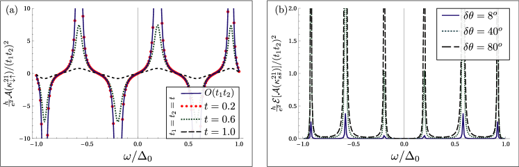
Figure 2: (a) Anti-symmetry in non-local differential conductance $\mathcal{A}(\kappa_{\downarrow\uparrow}^{21})/(t_{1}t_{2})^{2}$ as a function of $\omega$ for $L=3\xi$, $\theta_{1}=0$ and $\theta_{2}=\pi$. The solid dark blue line is the perturbative result in the order of $t_{1}t_{2}$ while other lines are the exact results for different values of $t_{1}=t_{2}=\{0.2,0.6,1.0\}$ (b) Exact numerical results (with $d\omega/\Delta_{0}=0.01$) for even-in-$\omega$ part of $\mathcal{A}(\kappa_{s_{2}s_{1}}^{21})/(t_{1}t_{2})^{2}$ as a function of $\omega$ for $x_{1}=\xi$, $x_{2}=2.5\xi$ ($L=3\xi$), $\{\theta_{1},\theta_{2}\}=\{\delta\theta,\pi+\delta\theta\}$, $t_{1}=t_{2}=0.2$ for different values of $\delta\theta=\{8^{o},40^{o},80^{o}\}$. The other parameters are taken to be $\mu=10\Delta_{0}$ and $\varphi_{21}=\pi/2$.

Using Landauer’s formula[70], we can calculate the differential conductance from $P_{1}$ to $P_{2}$, given by $\kappa_{\downarrow\uparrow}^{21}=\kappa_{ee,\downarrow\uparrow}^{21}-\kappa_{he,\downarrow\uparrow}^{21}$ and from $P_{2}$ to $P_{1}$, given by $\kappa_{\uparrow\downarrow}^{12}=\kappa_{ee,\uparrow\downarrow}^{12}-\kappa_{he,\uparrow\downarrow}^{12}$, where $\kappa_{p_{i}p_{j},s_{i}s_{j}}^{ij}=(e^{2}/h)|t_{p_{i}p_{j},s_{i}s_{j}}^{ij}|^{2}$ ($p_{i(j)}\in\{e,h\}$, $s_{i(j)}\in\{\uparrow,\downarrow\}$, $\{i,j\}\in\{1,2\}$). The difference between these two non-local differential conductances at energy (frequency) $\omega$ is given by:

$$\mathcal{A}(\kappa_{\downarrow\uparrow}^{21}) =\kappa_{\downarrow\uparrow}^{21}-\kappa_{\uparrow\downarrow}^{12},$$

$$=-\kappa_{he,\downarrow\uparrow}^{21}+\kappa_{he,\uparrow\downarrow}^{12},$$

$$\propto -|G^{r}_{he,\downarrow\uparrow}(x_{2},x_{1},\omega)|^{2}+|G^{r}_{he,\uparrow\downarrow}(x_{1},x_{2},\omega)|^{2},$$

$$\propto -|G^{r}_{he,\downarrow\uparrow}(x_{2},x_{1},\omega)|^{2}+|G^{a}_{he,\downarrow\uparrow}(x_{2},x_{1},-\omega)|^{2},$$

$$\propto ~{}\text{Re}[\,\mathcal{O}[G^{r}_{he,\downarrow\uparrow}(x_{2},x_{1},\omega)]\times\mathcal{E}[G^{r*}_{he,\downarrow\uparrow}(x_{2},x_{1},\omega)]\,].$$ (7)

where we have used the property $G^{r}_{he,s\bar{s}}(x,x^{\prime},\omega)=G^{a}_{he,\bar{s}s}(x^{\prime},x,-\omega)$ ($\{s,\bar{s}\}\in\{\uparrow,\downarrow\}$ and $s\neq\bar{s}$). Here we have used only retarded Green’s functions to express $\kappa$. However, a proof involving advanced Green’s functions follows in a similar way (See SM SectionB). Eq. (7) is anti-symmetric with respect to $\omega$, and if measured, it can be treated as a direct signature of odd-$\omega$ pairing subjected to the condition that even-$\omega$ pairing within the junction is non-zero. In Eq. (7), $\mathcal{O}$ and $\mathcal{E}$ denote the odd-in-$\omega$ and even-in-$\omega$ parts of the corresponding Green’s functions which are in turn directly related to odd-$\omega$ and even-$\omega$ pairing amplitudes respectively. Note that, the quantity in Eq. (7) can also be expressed as $\mathcal{B}(\kappa_{\downarrow\uparrow}^{21})=[\kappa_{\downarrow\uparrow}^{21}(\omega)-\kappa_{\downarrow\uparrow}^{21}(-\omega)]$. The voltage configuration necessary for measuring $\mathcal{A}(\kappa)$ and $\mathcal{B}(\kappa)$ is discussed above Eq. (2). Now, we will proceed to put the above qualitative discussion on firm grounds by evaluating the expression for various non-local, spin-resolved normal, and anomalous Green’s functions and expressing the spin-resolved Landauer conductance between the probes in terms of these quantities.

Results and discussions: The wave functions in different regions of the system can be obtained by diagonalizing the Hamiltonians in 3 and 4. By demanding the continuity of wave functions at $x=0,L$ and assuming that the incoming and outgoing plane wave amplitudes are related via Eq. (6) at $x=x_{1}$ and at $x=x_{2}$, one can arrive at the expressions for different non-local transmission amplitudes when an electron is injected through one of the probes, for arbitrary values of $\theta_{1}$ and $\theta_{2}$. These quantities can be expanded into the Taylor series with respect to $t_{1}$ and $t_{2}$ and, in the weak tunneling limit (i.e., in the lowest order of $t_{1}$ and $t_{2}$), can be re-expressed in terms of free (the term free refers to JJ in the absence of probes) Green’s functions as

$$t_{ee}^{21} =-it_{1}t_{2}e^{i(k_{e}^{P_{1}}x_{1}-k_{e}^{P_{2}}x_{2})}\left\{G^{r(a)}_{ee,\uparrow\uparrow}(x_{2}>x_{1},\omega)\cos{(\theta_{1}/2)}\cos{(\theta_{2}/2)}+G^{r(a)}_{ee,\downarrow\downarrow}(x_{2}>x_{1},\omega)\sin{(\theta_{1}/2)}\sin{(\theta_{2}/2)}\right\}\,,$$ (8)

$$t_{he}^{21} =it_{1}t_{2}e^{i(k_{e}^{P_{1}}x_{1}+k_{h}^{P_{2}}x_{2})}\left\{G^{r(a)}_{he,\downarrow\uparrow}(x_{2},x_{1},\omega)\cos{(\theta_{1}/2)\sin{(\theta_{2}/2)}}-G^{r(a)}_{he,\uparrow\downarrow}(x_{2},x_{1},\omega)\sin{(\theta_{1}/2)}\cos{(\theta_{2}/2)}\right\}\,,$$ (9)

$$t_{ee}^{12} =-it_{1}t_{2}e^{i(k_{e}^{P_{2}}x_{2}-k_{e}^{P_{1}}x_{1})}\left\{G^{r(a)}_{ee,\uparrow\uparrow}(x_{1}<x_{2},\omega)\cos{(\theta_{1}/2)}\cos{(\theta_{2}/2)}+G^{r(a)}_{ee,\downarrow\downarrow}(x_{1}<x_{2},\omega)\sin{(\theta_{1}/2)}\sin{(\theta_{2}/2)}\right\}\,,$$ (10)

$$t_{he}^{12} =it_{1}t_{2}e^{i(k_{e}^{P_{2}}x_{2}+k_{h}^{P_{1}}x_{1})}\left\{G^{r(a)}_{he,\downarrow\uparrow}(x_{1},x_{2},\omega)\sin{(\theta_{1}/2)}\cos{(\theta_{2}/2)}-G^{r(a)}_{he,\uparrow\downarrow}(x_{1},x_{2},\omega)\cos{(\theta_{1}/2)}\sin{(\theta_{2}/2)}\right\}.\,$$ (11)

Note that, TABLE. 1 is consistent with the general expressions derived in Eq. (8)- (11) (For details see SM Section C). For arbitrary $\theta_{1}$ and $\theta_{2}$, $\mathcal{A}(\kappa)$ will have contributions from interference effects between the spin channels and the electron-hole channels due to the presence of more than one Green’s function in the expressions of $t^{ij}_{p\bar{p}}$. The quantity $\mathcal{A}(\kappa_{\downarrow\uparrow}^{21})/(t_{1}t_{2})^{2}$ is plotted in FIG. 2(a) both in the perturbative (i.e., in the weak tunneling limit) and non-perturbative limit for $\{\theta_{1},\theta_{2}\}=\{0,\pi\}$. As we can see from the figure, the anti-symmetry feature continues to hold even in the non-perturbative limit. This is due to the fact that at $\theta_{1}(\theta_{2})=0$ or $\pi$, the spin-flip scattering process within the (normal region of) HES, becomes nonexistent as discussed below Eq. (5). As we deviate from $0$ and $\pi$, the interference contribution as discussed below Eq. (11) becomes finite, leading to deviation from perfectly anti-symmetric features. FIG. 2 (b) shows how the even-in-$\omega$ part of $\mathcal{A}(\kappa_{s\bar{s}}^{21})$ changes for $\{\theta_{1},\theta_{2}\}=\{\delta\theta,\pi+\delta\theta\}$. Note the different $y$-scale in FIGs. 2(a) and (b).

The detection of odd-frequency pairing through $\mathcal{A}(\kappa)$ does not require the probes $P_{1}$ and $P_{2}$ to be placed at different positions. This is due to the fact that the information of position enters into the calculation as pure phase contributions to $t^{ij}_{p\bar{p},s\bar{s}}$ ($\{s,\bar{s}\}\in\{\uparrow,\downarrow\}$, $s\neq\bar{s}$) in the weak tunneling limit. Lastly, note that, $\kappa_{he,\downarrow\uparrow}^{21}$ is related to the ABS corresponding to the shuttling of a Cooper pair from left to right, while $\kappa_{he,\uparrow\downarrow}^{12}$ is related to the ABS corresponding to the shuttling of Cooper pair in the opposite direction. Thus, in the weak tunneling limit, at $\varphi_{21}=0$ or $\pi$, (when these two ABS become degenerate), the differential conductances $\kappa_{he,\downarrow\uparrow}^{21}$ and $\kappa_{he,\uparrow\downarrow}^{12}$ becomes equal, leading to the vanishing of $\mathcal{A}(\kappa_{\downarrow\uparrow}^{21})$.

Acknowledgements: S.P. and A.M. acknowledge the Ministry of Education, India, and IISER Kolkata for funding.

Author contribution: S.P. and A.M. contributed equally to this work.

Supplemental Material A Derivation of scattering matrix

We start with the Hamiltonian $H=H_{\text{HES}}+\sum_{i\in\{1,2\}}H_{P_{i}}+H_{T}^{P_{i}}$ as mentioned below Eq. (5) in the main text. The equation of motion of an electron with spin $\alpha$, either within the HES or in the probes, can be written as

$$i\hbar\dot{\psi_{\alpha}}=[\psi_{\alpha},H].$$ (12)

For stationary state problem $\dot{\psi}_{\alpha}=0$ (here $\alpha\in\{\uparrow,\downarrow,\hat{n}_{i}\}$ as defined below Eq. (5) in the main text). Thus, one can solve the following equation[68]

$$\lim_{\epsilon\rightarrow x_{i}}\int_{-\epsilon}^{\epsilon}[\psi_{\alpha},H]dx=0,$$ (13)

to arrive at different matrix elements of $S^{e}$, as defined in Eq. (6) in the main text. which turns out to be of the following form:

$$\begin{pmatrix}S^{e}_{\uparrow\uparrow}&S^{e}_{\uparrow\downarrow}&S^{e}_{\uparrow\hat{n}_{i}}\\ S^{e}_{\downarrow\uparrow}&S^{e}_{\downarrow\downarrow}&S^{e}_{\downarrow\hat{n}_{i}}\\ S^{e}_{\hat{n}_{i}\uparrow}&S^{e}_{\hat{n}_{i}\downarrow}&S^{e}_{\hat{n}_{i}\hat{n}_{i}}\end{pmatrix}_{x=x_{i}}=\begin{pmatrix}\dfrac{4-t_{i}^{2}\cos(\theta_{i})}{4+t_{i}^{2}}&-\dfrac{t_{i}^{2}\sin(\theta_{i})}{4+t_{i}^{2}}&-\dfrac{4it_{i}\cos(\theta_{i}/2)}{4+t_{i}^{2}}\\ -\dfrac{t_{i}^{2}\sin(\theta_{i})}{4+t_{i}^{2}}&\dfrac{4+t_{i}^{2}\cos(\theta_{i})}{4+t_{i}^{2}}&-\dfrac{4it_{i}\sin(\theta_{i}/2)}{4+t_{i}^{2}}\\ -\dfrac{4it_{i}\cos(\theta_{i}/2)}{4+t_{i}^{2}}&-\dfrac{4it_{i}\sin(\theta_{i}/2)}{4+t_{i}^{2}}&\dfrac{4-t_{i}^{2}}{4+t_{i}^{2}}\end{pmatrix}.$$ (14)

Similar to Eq. (12) and (13), one can write the equation of motion for $\psi_{\alpha}^{\dagger}$. Particle-hole symmetry enables us to write the hole wave functions ($\psi_{\alpha}^{h}$) in terms of electron wave functions ($\psi_{\alpha}$) as

$$\psi^{h}_{\alpha}=\eta(\alpha)\psi_{\alpha}^{\dagger},$$ (15)

where we have considered $\eta(\alpha)=-1$ for $\alpha=\uparrow$ (within the HES) and $\eta=1$ otherwise. Note that, this convention is consistent with the particle-hole symmetry of the Nambu basis as in Eq. (3) in the main text. In a similar spirit as in Eq. (6) of the main text, one can define the scattering matrix of the hole, which turns out to be of the following form:

$$\begin{pmatrix}S^{h}_{\uparrow\uparrow}&S^{h}_{\uparrow\downarrow}&S^{h}_{\uparrow\hat{n}_{i}}\\ S^{h}_{\downarrow\uparrow}&S^{h}_{\downarrow\downarrow}&S^{h}_{\downarrow\hat{n}_{i}}\\ S^{h}_{\hat{n}_{i}\uparrow}&S^{h}_{\hat{n}_{i}\downarrow}&S^{h}_{\hat{n}_{i}\hat{n}_{i}}\end{pmatrix}_{x=x_{i}}=\begin{pmatrix}\dfrac{4-t_{i}^{2}\cos(\theta_{i})}{4+t_{i}^{2}}&\dfrac{t_{i}^{2}\sin(\theta_{i})}{4+t_{i}^{2}}&-\dfrac{4it_{i}\cos(\theta_{i}/2)}{4+t_{i}^{2}}\\ \dfrac{t_{i}^{2}\sin(\theta_{i})}{4+t_{i}^{2}}&\dfrac{4+t_{i}^{2}\cos(\theta_{i})}{4+t_{i}^{2}}&\dfrac{4it_{i}\sin(\theta_{i}/2)}{4+t_{i}^{2}}\\ -\dfrac{4it_{i}\cos(\theta_{i}/2)}{4+t_{i}^{2}}&\dfrac{4it_{i}\sin(\theta_{i}/2)}{4+t_{i}^{2}}&\dfrac{4-t_{i}^{2}}{4+t_{i}^{2}}\end{pmatrix}.$$ (16)

Supplemental Material B Derivation of Eq. (7) in terms of pairing amplitudes

One can decompose the spin symmetry of retarded (advanced) Green’s function $G^{r(a)}_{he}$ as[71]

$$G_{he}^{r(a)}(x,x^{\prime},\omega)=\begin{pmatrix}G_{he,\downarrow\uparrow}^{r(a)}(x,x^{\prime},\omega)&G_{he,\downarrow\downarrow}^{r(a)}(x,x^{\prime},\omega)\\ G_{he,\uparrow\uparrow}^{r(a)}(x,x^{\prime},\omega)&G_{he,\uparrow\downarrow}^{r(a)}(x,x^{\prime},\omega)\end{pmatrix}=\sum_{j=0}^{3}f_{j}^{r(a)}(x,x^{\prime},\omega)\sigma_{j}$$ (17)

where $f^{r(a)}_{0}$, $f^{r(a)}_{1,2}$, $f^{r(a)}_{3}$ corresponds to spin-singlet, equal spin-triplet and mixed spin-triplet retarded (advanced) pairing amplitudes respectively. The relation between $f^{r}$ and $f^{a}$ is dictated by Fermi-Dirac statistics and is given by

$$f_{0}^{r}(x,x^{\prime},\omega)=f_{0}^{a}(x^{\prime},x,-\omega),\qquad f_{j}^{r}(x,x^{\prime},\omega)=-f_{j}^{a}(x^{\prime},x,-\omega),$$ (18)

where $j\in\{1,2,3\}$. The off-diagonal elements in Eq. (17) are zero for our case. Thus, we get

$$G_{he,\downarrow\uparrow}^{r(a)}(x,x^{\prime},\omega)=f_{0}^{r(a)}(x,x^{\prime},\omega)+f_{3}^{r(a)}(x,x^{\prime},\omega),\qquad G_{he,\uparrow\downarrow}^{r(a)}(x,x^{\prime},\omega)=f_{0}^{r(a)}(x,x^{\prime},\omega)-f_{3}^{r(a)}(x,x^{\prime},\omega).$$ (19)

Using Eq. (18) and (19), it can be easily shown that

$$G_{he,\downarrow\uparrow}^{r}(x,x^{\prime},\omega)=G_{he,\uparrow\downarrow}^{a}(x^{\prime},x,-\omega),\qquad G_{he,\uparrow\downarrow}^{r}(x,x^{\prime},\omega)=G_{he,\downarrow\uparrow}^{a}(x^{\prime},x,-\omega).$$ (20)

The second identity in Eq. (20) has been used to arrive at Eq. (7) in the main text. Alternatively, one can use the particle-hole symmetry of the Green’s function $\mathcal{P}G^{r}(x,x^{\prime},\omega)\mathcal{P}^{-1}=-G^{r}(x,x^{\prime},-\omega)$, where $\mathcal{P}=\sigma_{y}\tau_{y}\mathcal{K}$ with $\mathcal{K}$ being the operation of complex conjugation, to arrive at the identity

$$G_{he,\uparrow\downarrow}^{r}(x,x^{\prime},\omega)=G_{eh,\uparrow\downarrow}^{r*}(x,x^{\prime},-\omega).$$ (21)

Again, from identity $G^{a}(x,x^{\prime},\omega)=[G^{r}(x^{\prime},x,\omega)]^{\dagger}$, we have

$$G_{eh,\uparrow\downarrow}^{r*}(x,x^{\prime},-\omega)=G_{he,\downarrow\uparrow}^{a}(x^{\prime},x,-\omega).$$ (22)

Thus, by equating (21) and (22), we arrive at the same result.

Now, the quantity we are interested in is $-|G^{r}_{he,\downarrow\uparrow}(x_{2},x_{1},\omega)|^{2}+|G^{a}_{he,\downarrow\uparrow}(x_{2},x_{1},-\omega)|^{2}$. Using Eq. (19) we can write

$$\mathcal{Q} =-|G^{r}_{he,\downarrow\uparrow}(x_{2},x_{1},\omega)|^{2}+|G^{a}_{he,\downarrow\uparrow}(x_{2},x_{1},-\omega)|^{2}$$

$$=-|f_{0}^{r}(x_{2},x_{1},\omega)+f_{3}^{r}(x_{2},x_{1},\omega)|^{2}+|f_{0}^{a}(x_{2},x_{1},-\omega)+f_{3}^{a}(x_{2},x_{1},-\omega)|^{2}.$$ (23)

From this point onwards, we shall drop $(x_{2},x_{1},\pm\omega)$ in the parentheses, and it will be understood that advanced pairing amplitudes ($f^{a}$) correspond to $-\omega$. Also, it will be helpful to introduce the even ($f^{r,E}$) and odd parts ($f^{r,O}$) of the pairing amplitudes at this stage, defined as

$$f^{r,E(O)}=\dfrac{f^{r}\pm f^{a}}{2}\qquad f^{r(a)}=f^{r,E}\pm f^{r,O}$$ (24)

Thus, from Eq. (23), using Eq. (24), we get,

$$-\mathcal{Q}$$

$$=(f_{0}^{r}+f_{3}^{r})(f_{0}^{r*}+f_{3}^{r*})-(f_{0}^{a}+f_{3}^{a})(f_{0}^{a*}+f_{3}^{a*})$$

$$=\left(f_{0}^{r}f_{0}^{r*}+f_{3}^{r}f_{3}^{r*}+f_{0}^{r}f_{3}^{r*}+f_{0}^{r*}f_{3}^{r}-(f_{0}^{a}f_{0}^{a*}+f_{3}^{a}f_{3}^{a*}+f_{0}^{a}f_{3}^{a*}+f_{0}^{a*}f_{3}^{a})\right)$$

$$=2\left((f_{0}^{r,O}+f_{3}^{r,O})(f_{0}^{r,E*}+f_{3}^{r,E*})+(f_{0}^{r,O*}+f_{3}^{r,O*})(f_{0}^{r,E}+f_{3}^{r,E})\right)$$

$$=4\,\text{Re}\left[\left(f_{0}^{r,O}+f_{3}^{r,O}\right)\left(f_{0}^{r,E*}+f_{3}^{r,E*}\right)\right]$$

$$=4\,\text{Re}\left[\,\mathcal{O}[G^{r}_{he,\downarrow\uparrow}]\times\mathcal{E}[G^{r*}_{he,\downarrow\uparrow}]\,\right]$$ (25)

Thus, $-|G^{r}_{he,\downarrow\uparrow}(x_{2},x_{1},\omega)|^{2}+|G^{a}_{he,\downarrow\uparrow}(x_{2},x_{1},-\omega)|^{2}\propto\text{Re}\left[\,\mathcal{O}[G^{r}_{he,\downarrow\uparrow}(x_{2},x_{1},-\omega)]\times\mathcal{E}[G^{r*}_{he,\downarrow\uparrow}(x_{2},x_{1},-\omega)]\,\right]$ which has been used to derive Eq. (7) in the main text. We can also use $\mathcal{A}(\kappa_{\downarrow\uparrow}^{21})\propto-|G^{a}_{he,\downarrow\uparrow}(x_{2},x_{1},\omega)|^{2}+|G^{a}_{he,\uparrow\downarrow}(x_{1},x_{2},\omega)|^{2}$ in Eq. (7) of the main text instead of retarded Green’s functions. In that case, we would have arrived at the same expression as Eq. (25) with $G^{r}_{he,\downarrow\uparrow}$ replaced by $G^{a}_{he,\downarrow\uparrow}$. Eq. (25) also justifies our statement that $\mathcal{A}(\kappa_{\downarrow\uparrow}^{21})$ is anti-symmetric with respect to $\omega$ and can be treated as a direct signature of odd-$\omega$ pairing when even-$\omega$ pairing is non-zero.

Supplemental Material C Non-local transmission amplitudes

Different non-local (intra-probe) transmission amplitudes for the system in FIG. 1, when an electron is injected through one of the probes, can be calculated by the standard process as discussed in the main text before Eq. (8). The lowest order in $t_{1}$ and $t_{2}$, having non-zero terms in the Taylor series expansion of these quantities, is $O(t_{1}^{\,1}t_{2}^{\,1})$. Any lower order would physically mean that at least one of the probes is disconnected from the HES, resulting in the absence of non-local transmission amplitudes. In this lowest order, different transmission amplitudes read as

$$t_{ee}^{21} =t_{1}t_{2}e^{i(k_{e}^{P_{1}}x_{1}-k_{e}^{P_{2}}x_{2})}\left(-\dfrac{e^{ik_{e}(x_{2}-x_{1})}\cos(\frac{\theta_{1}}{2})\cos(\frac{\theta_{2}}{2})}{1-e^{i(k_{e}L-k_{h}L-2\rho-\varphi_{21})}}+\dfrac{e^{ik_{e}(x_{1}-x_{2})}\sin(\frac{\theta_{1}}{2})\sin(\frac{\theta_{2}}{2})}{1-e^{-i(k_{e}L-k_{h}L-2\rho+\varphi_{21})}}\right),$$ (26)

$$t_{he}^{21} =t_{1}t_{2}e^{i(k_{e}^{P_{1}}x_{1}+k_{h}^{P_{2}}x_{2})}\left(-\dfrac{e^{i(k_{e}x_{1}-k_{h}x_{2}-\rho)}\sin(\frac{\theta_{1}}{2})\cos(\frac{\theta_{2}}{2})}{1-e^{i(k_{e}L-k_{h}L-2\rho+\varphi_{21})}}-\dfrac{e^{-i(k_{e}x_{1}-k_{h}x_{2}-\rho)}\cos(\frac{\theta_{1}}{2})\sin(\frac{\theta_{2}}{2})}{1-e^{-i(k_{e}L-k_{h}L-2\rho-\varphi_{21})}}\right),$$ (27)

$$t_{ee}^{12} =t_{1}t_{2}e^{i(k_{e}^{P_{2}}x_{2}-k_{e}^{P_{1}}x_{1})}\left(\dfrac{e^{ik_{e}(x_{1}-x_{2})}\cos(\frac{\theta_{1}}{2})\cos(\frac{\theta_{2}}{2})}{1-e^{-i(k_{e}L-k_{h}L-2\rho-\varphi_{21})}}-\dfrac{e^{ik_{e}(x_{2}-x_{1})}\sin(\frac{\theta_{1}}{2})\sin(\frac{\theta_{2}}{2})}{1-e^{i(k_{e}L-k_{h}L-2\rho+\varphi_{21})}}\right),$$ (28)

$$t_{he}^{12} =t_{1}t_{2}e^{i(k_{e}^{P_{2}}x_{2}+k_{h}^{P_{1}}x_{1})}\left(-\dfrac{e^{-i(k_{e}x_{2}-k_{h}x_{1}-\rho)}\sin(\frac{\theta_{1}}{2})\cos(\frac{\theta_{2}}{2})}{1-e^{-i(k_{e}L-k_{h}L-2\rho-\varphi_{21})}}-\dfrac{e^{i(k_{e}x_{2}-k_{h}x_{1}-\rho)}\cos(\frac{\theta_{1}}{2})\sin(\frac{\theta_{2}}{2})}{1-e^{i(k_{e}L-k_{h}L-2\rho+\varphi_{21})}}\right),$$ (29)

where $\rho=\arccos(\omega/\Delta_{0})$ (for $|\omega|\leq\Delta_{0})$ and $k_{e,h}=\mu\pm\omega$ are the wave-vectors in the metallic region while $k_{e,h}^{P_{1},P_{2}}$ are the corresponding wave-vectors in the tunnelling probes $P_{1}$ and $P_{2}$. The quantities $t_{ee}^{21(12)}$ and $t_{he}^{21(12)}$ are electron and hole transmission amplitudes from $P_{1}(P_{2})$ to $P_{2}(P_{1})$.

Now, the expressions for different relevant free Green’s functions within the normal region of a JJ based on HES are given as[38]

$$G^{r}_{ee,\uparrow\uparrow}(x_{2}>x_{1},\omega) =\frac{1}{i}\frac{e^{ik_{e}(x_{2}-x_{1})}}{1-e^{i(k_{e}L-k_{h}L-2\rho-\varphi_{21})}}=G^{a}_{ee,\uparrow\uparrow}(x_{2}>x_{1},\omega),$$ (30)

$$G^{r}_{ee,\uparrow\uparrow}(x_{1}<x_{2},\omega) =\frac{1}{i}\frac{-e^{ik_{e}(x_{1}-x_{2})}}{1-e^{-i(k_{e}L-k_{h}L-2\rho-\varphi_{21})}}=G^{a}_{ee,\uparrow\uparrow}(x_{1}<x_{2},\omega),$$ (31)

$$G^{r}_{ee,\downarrow\downarrow}(x_{2}>x_{1},\omega) =\frac{1}{i}\frac{-e^{ik_{e}(x_{1}-x_{2})}}{1-e^{-i(k_{e}L-k_{h}L-2\rho+\varphi_{21})}}=G^{a}_{ee,\downarrow\downarrow}(x_{2}>x_{1},\omega),$$ (32)

$$G^{r}_{ee,\downarrow\downarrow}(x_{1}<x_{2},\omega) =\frac{1}{i}\frac{e^{ik_{e}(x_{2}-x_{1})}}{1-e^{i(k_{e}L-k_{h}L-2\rho+\varphi_{21})}}=G^{a}_{ee,\downarrow\downarrow}(x_{1}<x_{2},\omega),$$ (33)

$$G^{r}_{he,\downarrow\uparrow}(x,x^{\prime},\omega) =\frac{1}{i}\frac{-e^{-i(k_{e}x^{\prime}-k_{h}x-\rho)}}{1-e^{-i(k_{e}L-k_{h}L-2\rho-\varphi_{21})}}=G^{a}_{he,\downarrow\uparrow}(x,x^{\prime},\omega),$$ (34)

$$G^{r}_{he,\uparrow\downarrow}(x,x^{\prime},\omega) =\frac{1}{i}\frac{e^{i(k_{e}x^{\prime}-k_{h}x-\rho)}}{1-e^{i(k_{e}L-k_{h}L-2\rho+\varphi_{21})}}=G^{a}_{he,\uparrow\downarrow}(x,x^{\prime},\omega),$$ (35)

($\{x,x^{\prime}\}\in\{x_{1},x_{2}\}$). Now, one can use Eq. (30)-(35) and Eq. (26)-(29) to re-express the transmission amplitudes in terms of Green’s functions to arrive at Eq. (8)-(11) in the main text.

References

• Bardeen et al. [1957] J. Bardeen, L. N. Cooper, and J. R. Schrieffer, Theory of superconductivity, Phys. Rev. 108, 1175 (1957).
• Berezinskii [1974] V. Berezinskii, New model of the anisotropic phase of superfluid he3, JETP Lett 20 (1974).
• Sigrist and Ueda [1991] M. Sigrist and K. Ueda, Phenomenological theory of unconventional superconductivity, Rev. Mod. Phys. 63, 239 (1991).
• Linder and Balatsky [2019] J. Linder and A. V. Balatsky, Odd-frequency superconductivity, Rev. Mod. Phys. 91, 045005 (2019).
• Tanaka et al. [2011] Y. Tanaka, M. Sato, and N. Nagaosa, Symmetry and topology in superconductors–odd-frequency pairing and edge states–, Journal of the Physical Society of Japan 81, 011013 (2011).
• Cayao et al. [2020] J. Cayao, C. Triola, and A. M. Black-Schaffer, Odd-frequency superconducting pairing in one-dimensional systems, The European Physical Journal Special Topics 229, 545 (2020).
• Kirkpatrick and Belitz [1991] T. R. Kirkpatrick and D. Belitz, Disorder-induced triplet superconductivity, Phys. Rev. Lett. 66, 1533 (1991).
• Belitz and Kirkpatrick [1992] D. Belitz and T. R. Kirkpatrick, Even-parity spin-triplet superconductivity in disordered electronic systems, Phys. Rev. B 46, 8393 (1992).
• Balatsky and Abrahams [1992] A. Balatsky and E. Abrahams, New class of singlet superconductors which break the time reversal and parity, Phys. Rev. B 45, 13125 (1992).
• Emery and Kivelson [1992] V. J. Emery and S. Kivelson, Mapping of the two-channel kondo problem to a resonant-level model, Phys. Rev. B 46, 10812 (1992).
• Balatsky and Boncˇa [1993] A. V. Balatsky and J. Boncˇa, Even- and odd-frequency pairing correlations in the one-dimensional t-j-h model: A comparative study, Phys. Rev. B 48, 7445 (1993).
• Bulut et al. [1993] N. Bulut, D. J. Scalapino, and S. R. White, Effective particle-particle interaction in the two-dimensional hubbard model, Phys. Rev. B 47, 6157 (1993).
• Coleman et al. [1993] P. Coleman, E. Miranda, and A. Tsvelik, Possible realization of odd-frequency pairing in heavy fermion compounds, Phys. Rev. Lett. 70, 2960 (1993).
• Kashuba et al. [2017] O. Kashuba, B. Sothmann, P. Burset, and B. Trauzettel, Majorana stm as a perfect detector of odd-frequency superconductivity, Phys. Rev. B 95, 174516 (2017).
• Schemm et al. [2014] E. Schemm, W. Gannon, C. Wishne, W. Halperin, and A. Kapitulnik, Observation of broken time-reversal symmetry in the heavy-fermion superconductor upt3, Science 345, 190 (2014).
• Komendová and Black-Schaffer [2017] L. Komendová and A. M. Black-Schaffer, Odd-frequency superconductivity in ${\mathrm{sr}}_{2}{\mathrm{ruo}}_{4}$ measured by kerr rotation, Phys. Rev. Lett. 119, 087001 (2017).
• Di Bernardo et al. [2015a] A. Di Bernardo, Z. Salman, X. L. Wang, M. Amado, M. Egilmez, M. G. Flokstra, A. Suter, S. L. Lee, J. H. Zhao, T. Prokscha, E. Morenzoni, M. G. Blamire, J. Linder, and J. W. A. Robinson, Intrinsic paramagnetic meissner effect due to $s$-wave odd-frequency superconductivity, Phys. Rev. X 5, 041021 (2015a).
• Bergeret et al. [2001a] F. S. Bergeret, A. F. Volkov, and K. B. Efetov, Josephson current in superconductor-ferromagnet structures with a nonhomogeneous magnetization, Phys. Rev. B 64, 134506 (2001a).
• Alidoust et al. [2014] M. Alidoust, K. Halterman, and J. Linder, Meissner effect probing of odd-frequency triplet pairing in superconducting spin valves, Phys. Rev. B 89, 054508 (2014).
• Krieger et al. [2020] J. A. Krieger, A. Pertsova, S. R. Giblin, M. Döbeli, T. Prokscha, C. W. Schneider, A. Suter, T. Hesjedal, A. V. Balatsky, and Z. Salman, Proximity-induced odd-frequency superconductivity in a topological insulator, Phys. Rev. Lett. 125, 026802 (2020).
• Yokoyama et al. [2011] T. Yokoyama, Y. Tanaka, and N. Nagaosa, Anomalous meissner effect in a normal-metal–superconductor junction with a spin-active interface, Phys. Rev. Lett. 106, 246601 (2011).
• Perrin et al. [2020] V. Perrin, F. L. N. Santos, G. C. Ménard, C. Brun, T. Cren, M. Civelli, and P. Simon, Unveiling odd-frequency pairing around a magnetic impurity in a superconductor, Phys. Rev. Lett. 125, 117003 (2020).
• Kuzmanovski et al. [2020] D. Kuzmanovski, R. S. Souto, and A. V. Balatsky, Odd-frequency superconductivity near a magnetic impurity in a conventional superconductor, Phys. Rev. B 101, 094505 (2020).
• Kornich et al. [2021] V. Kornich, F. Schlawin, M. A. Sentef, and B. Trauzettel, Direct detection of odd-frequency superconductivity via time- and angle-resolved photoelectron fluctuation spectroscopy, Phys. Rev. Res. 3, L042034 (2021).
• Chakraborty and Black-Schaffer [2022] D. Chakraborty and A. M. Black-Schaffer, Quasiparticle interference as a direct experimental probe of bulk odd-frequency superconducting pairing, Phys. Rev. Lett. 129, 247001 (2022).
• Abrahams et al. [1995] E. Abrahams, A. Balatsky, D. J. Scalapino, and J. R. Schrieffer, Properties of odd-gap superconductors, Phys. Rev. B 52, 1271 (1995).
• Bergeret et al. [2001b] F. S. Bergeret, A. F. Volkov, and K. B. Efetov, Long-range proximity effects in superconductor-ferromagnet structures, Phys. Rev. Lett. 86, 4096 (2001b).
• Bergeret et al. [2003] F. S. Bergeret, A. F. Volkov, and K. B. Efetov, Manifestation of triplet superconductivity in superconductor-ferromagnet structures, Phys. Rev. B 68, 064513 (2003).
• Bergeret et al. [2005] F. S. Bergeret, A. F. Volkov, and K. B. Efetov, Odd triplet superconductivity and related phenomena in superconductor-ferromagnet structures, Rev. Mod. Phys. 77, 1321 (2005).
• Eschrig et al. [2003] M. Eschrig, J. Kopu, J. C. Cuevas, and G. Schön, Theory of half-metal/superconductor heterostructures, Phys. Rev. Lett. 90, 137003 (2003).
• Volkov et al. [2006] A. F. Volkov, A. Anishchanka, and K. B. Efetov, Odd triplet superconductivity in a superconductor/ferromagnet system with a spiral magnetic structure, Phys. Rev. B 73, 104412 (2006).
• Yokoyama et al. [2007] T. Yokoyama, Y. Tanaka, and A. A. Golubov, Manifestation of the odd-frequency spin-triplet pairing state in diffusive ferromagnet/superconductor junctions, Phys. Rev. B 75, 134510 (2007).
• Tanaka et al. [2007] Y. Tanaka, Y. Tanuma, and A. A. Golubov, Odd-frequency pairing in normal-metal/superconductor junctions, Phys. Rev. B 76, 054522 (2007).
• Black-Schaffer and Balatsky [2012] A. M. Black-Schaffer and A. V. Balatsky, Odd-frequency superconducting pairing in topological insulators, Phys. Rev. B 86, 144506 (2012).
• Black-Schaffer and Balatsky [2013] A. M. Black-Schaffer and A. V. Balatsky, Proximity-induced unconventional superconductivity in topological insulators, Phys. Rev. B 87, 220506 (2013).
• Crépin et al. [2015] F. m. c. Crépin, P. Burset, and B. Trauzettel, Odd-frequency triplet superconductivity at the helical edge of a topological insulator, Phys. Rev. B 92, 100507 (2015).
• Burset et al. [2015] P. Burset, B. Lu, G. Tkachov, Y. Tanaka, E. M. Hankiewicz, and B. Trauzettel, Superconducting proximity effect in three-dimensional topological insulators in the presence of a magnetic field, Phys. Rev. B 92, 205424 (2015).
• Cayao and Black-Schaffer [2017] J. Cayao and A. M. Black-Schaffer, Odd-frequency superconducting pairing and subgap density of states at the edge of a two-dimensional topological insulator without magnetism, Phys. Rev. B 96, 155426 (2017).
• Hwang et al. [2018] S.-Y. Hwang, P. Burset, and B. Sothmann, Odd-frequency superconductivity revealed by thermopower, Phys. Rev. B 98, 161408 (2018).
• Cayao and Black-Schaffer [2018] J. Cayao and A. M. Black-Schaffer, Odd-frequency superconducting pairing in junctions with rashba spin-orbit coupling, Phys. Rev. B 98, 075425 (2018).
• Linder et al. [2010] J. Linder, A. Sudbø, T. Yokoyama, R. Grein, and M. Eschrig, Signature of odd-frequency pairing correlations induced by a magnetic interface, Phys. Rev. B 81, 214504 (2010).
• Linder et al. [2009] J. Linder, T. Yokoyama, A. Sudbø, and M. Eschrig, Pairing symmetry conversion by spin-active interfaces in magnetic normal-metal–superconductor junctions, Phys. Rev. Lett. 102, 107008 (2009).
• Pal and Benjamin [2021] S. Pal and C. Benjamin, Exciting odd-frequency equal-spin triplet correlations at metal-superconductor interfaces, Phys. Rev. B 104, 054519 (2021).
• Tamura et al. [2023] S. Tamura, Y. Tanaka, and T. Yokoyama, Generation of polarized spin-triplet cooper pairings by magnetic barriers in superconducting junctions, Phys. Rev. B 107, 054501 (2023).
• Tanaka and Golubov [2007] Y. Tanaka and A. A. Golubov, Theory of the proximity effect in junctions with unconventional superconductors, Phys. Rev. Lett. 98, 037003 (2007).
• Eschrig et al. [2007] M. Eschrig, T. Löfwander, T. Champel, J. Cuevas, J. Kopu, and G. Schön, Symmetries of pairing correlations in superconductor–ferromagnet nanostructures, Journal of Low Temperature Physics 147, 457 (2007).
• Volkov et al. [2003] A. F. Volkov, F. S. Bergeret, and K. B. Efetov, Odd triplet superconductivity in superconductor-ferromagnet multilayered structures, Phys. Rev. Lett. 90, 117006 (2003).
• Fominov et al. [2007] Y. V. Fominov, A. F. Volkov, and K. B. Efetov, Josephson effect due to the long-range odd-frequency triplet superconductivity in $\mathrm{S}\mathrm{F}\mathrm{S}$ junctions with néel domain walls, Phys. Rev. B 75, 104509 (2007).
• Buzdin [2005] A. I. Buzdin, Proximity effects in superconductor-ferromagnet heterostructures, Rev. Mod. Phys. 77, 935 (2005).
• Tsintzis et al. [2019] A. Tsintzis, A. M. Black-Schaffer, and J. Cayao, Odd-frequency superconducting pairing in kitaev-based junctions, Phys. Rev. B 100, 115433 (2019).
• Asano and Tanaka [2013] Y. Asano and Y. Tanaka, Majorana fermions and odd-frequency cooper pairs in a normal-metal nanowire proximity-coupled to a topological superconductor, Phys. Rev. B 87, 104513 (2013).
• Kuzmanovski and Black-Schaffer [2017] D. Kuzmanovski and A. M. Black-Schaffer, Multiple odd-frequency superconducting states in buckled quantum spin hall insulators with time-reversal symmetry, Phys. Rev. B 96, 174509 (2017).
• Fleckenstein et al. [2018] C. Fleckenstein, N. T. Ziani, and B. Trauzettel, Conductance signatures of odd-frequency superconductivity in quantum spin hall systems using a quantum point contact, Phys. Rev. B 97, 134523 (2018).
• Triola and Balatsky [2016] C. Triola and A. V. Balatsky, Odd-frequency superconductivity in driven systems, Phys. Rev. B 94, 094518 (2016).
• Triola and Balatsky [2017] C. Triola and A. V. Balatsky, Pair symmetry conversion in driven multiband superconductors, Phys. Rev. B 95, 224518 (2017).
• Cayao et al. [2022] J. Cayao, P. Dutta, P. Burset, and A. M. Black-Schaffer, Phase-tunable electron transport assisted by odd-frequency cooper pairs in topological josephson junctions, Phys. Rev. B 106, L100502 (2022).
• Dutta and Black-Schaffer [2019] P. Dutta and A. M. Black-Schaffer, Signature of odd-frequency equal-spin triplet pairing in the josephson current on the surface of weyl nodal loop semimetals, Phys. Rev. B 100, 104511 (2019).
• Seoane Souto et al. [2020] R. Seoane Souto, D. Kuzmanovski, and A. V. Balatsky, Signatures of odd-frequency pairing in the josephson junction current noise, Phys. Rev. Res. 2, 043193 (2020).
• Khaire et al. [2010] T. S. Khaire, M. A. Khasawneh, W. P. Pratt, and N. O. Birge, Observation of spin-triplet superconductivity in co-based josephson junctions, Phys. Rev. Lett. 104, 137002 (2010).
• Di Bernardo et al. [2015b] A. Di Bernardo, S. Diesch, Y. Gu, J. Linder, G. Divitini, C. Ducati, E. Scheer, M. G. Blamire, and J. W. Robinson, Signature of magnetic-dependent gapless odd frequency states at superconductor/ferromagnet interfaces, Nature communications 6, 8053 (2015b).
• Das and Rao [2011] S. Das and S. Rao, Spin-polarized scanning-tunneling probe for helical luttinger liquids, Phys. Rev. Lett. 106, 236403 (2011).
• Fu and Kane [2009] L. Fu and C. L. Kane, Josephson current and noise at a superconductor/quantum-spin-hall-insulator/superconductor junction, Phys. Rev. B 79, 161408 (2009).
• Fu and Kane [2008] L. Fu and C. L. Kane, Superconducting proximity effect and majorana fermions at the surface of a topological insulator, Phys. Rev. Lett. 100, 096407 (2008).
• Kane and Mele [2005] C. L. Kane and E. J. Mele, Quantum spin hall effect in graphene, Phys. Rev. Lett. 95, 226801 (2005).
• Calzona and Trauzettel [2019] A. Calzona and B. Trauzettel, Moving majorana bound states between distinct helical edges across a quantum point contact, Phys. Rev. Res. 1, 033212 (2019).
• Mukhopadhyay and Das [2021] A. Mukhopadhyay and S. Das, Thermal signature of the majorana fermion in a josephson junction, Phys. Rev. B 103, 144502 (2021).
• Mukhopadhyay and Das [2022] A. Mukhopadhyay and S. Das, Thermal bias induced charge current in a josephson junction: From ballistic to disordered, Phys. Rev. B 106, 075421 (2022).
• Wadhawan et al. [2018] D. Wadhawan, K. Roychowdhury, P. Mehta, and S. Das, Multielectron geometric phase in intensity interferometry, Phys. Rev. B 98, 155113 (2018).
• Note [1] The azimuthal angle is of no consequence, e.g., it can also be assumed in the $z-y$ plane.
• Pershoguba et al. [2019] S. S. Pershoguba, T. Veness, and L. I. Glazman, Landauer formula for a superconducting quantum point contact, Phys. Rev. Lett. 123, 067001 (2019).
• Keidel et al. [2020] F. Keidel, S.-Y. Hwang, B. Trauzettel, B. Sothmann, and P. Burset, On-demand thermoelectric generation of equal-spin cooper pairs, Phys. Rev. Res. 2, 022019 (2020).
• Note [2] This form of Green’s function is due to our particular choice of basis. Also, note that, this decomposition is different from that used in Phys.Rev.B 96, 155426(2017) and is similar to Eq. (S.39) of the Supplemental Material of Phys. Rev. Research 2, 022019(R)(2020).